

Submitted:
07 August 2026
Posted:
07 August 2026
You are already at the latest version
Abstract
Accurate multi-step traffic flow forecasting requires dynamic spatial modeling and adaptation to heterogeneous temporal and node-level patterns. This study proposes FAMoE-ST, a hierarchically frozen attention network with a hybrid-memory mixture of experts. Historical flow and temporal and node context are encoded as sensor tokens and processed by a six-layer Transformer initialized from GPT-2. To remove dependence on arbitrary sensor indexing, causal masking is replaced by all-to-all bidirectional spatial attention, and all nodes share the zero GPT position ID. The lower four blocks are frozen, whereas the upper two blocks are adapted and their feed-forward networks are replaced by four-expert modules. A linear router is fused with a 32-slot memory router; each token retrieves four slots and activates two experts. With 12 observations predicting the next 12 steps, FAMoE-ST achieves MAE/RMSE/MAPE values of 18.55/30.35/12.91% on PEMS04 and 14.57/24.08/9.71% on PEMS08. Relative to ST-LLM, MAE decreases by 6.97% and 7.39%, respectively. Ablations show complementary benefits from restricted adaptation, sparse experts, and memory routing. A parameter-matched control further indicates that the gains are not attributable solely to stored capacity, although the experiments do not isolate the effect of GPT-2 pretraining.
Keywords:
traffic flow forecasting
; intelligent transportation systems
; GPT-style Transformer
; mixture of experts
; hierarchical freezing
; memory routing
1. Introduction
Traffic flow forecasting estimates future traffic states from historical roadside-sensor observations and supports signal control, route planning, congestion warning, and traffic guidance. The task is difficult because traffic dynamics are coupled across both space and time. Dependencies between nearby and distant sensors change as congestion propagates, while daily and weekly periodicity interacts with incidents, weather, and localized demand surges. A reliable multi-node, multi-step forecaster must therefore represent dynamic spatial interactions, multiscale temporal variation, and heterogeneous node behavior, and must remain stable at long horizons and under high-flow conditions.
Recent task-specific models have improved traffic propagation modeling through graph neural differential equations, spatiotemporal fusion, and dynamic graph decoupling [1,2,3,4]. STID, STEP, PDFormer, and STAEformer further strengthen multi-step forecasting through identity embeddings, self-supervised pretraining, propagation-delay modeling, and adaptive spatiotemporal embeddings [5,6,7,8], whereas TESTAM uses a mixture of experts to accommodate changes in traffic regimes [9]. These methods provide effective inductive biases, but many rely on task-specific graph construction or specialized architectural components, which can complicate adaptation across datasets and operating conditions.
A complementary line of research repurposes large pretrained or generally structured sequence models for traffic and time-series forecasting. ST-LLM introduces a GPT-style backbone into traffic prediction [10], while One Fits All, Time-LLM, zero-shot language-model forecasting, LLM4TS, TimesFM, Chronos, and MOMENT explore input mapping, reprogramming, or foundation-model pretraining [11,12,13,14,15,16,17]. PatchTST and TimesNet likewise demonstrate the value of generic sequence architectures for long-range and multiscale patterns [18,19]. However, language tokens and traffic measurements differ in semantics, distribution, and dependency structure. In this study, GPT-2 supplies the initial Transformer weights and block structure; beneficial transfer of linguistic knowledge is not assumed. Establishing such transfer would require a randomly initialized isomorphic backbone under the same training protocol. Full adaptation provides flexibility but increases optimization cost and the risk of unstable updates, whereas complete freezing can underfit the target domain. Parameter-efficient methods such as LoRA and P-Tuning address a related trade-off by restricting the trainable parameter space [20,21]. In parallel, conditional-computation models expand representational capacity through sparse or soft expert assignment [22,23,24,25], yet routers driven only by the current input can be sensitive to short-lived noise and imbalanced token allocation. A unified design that controls backbone adaptation and combines instantaneous traffic states with cross-batch routing references remains underexplored.
To address these limitations, we propose FAMoE-ST, which combines depth-controlled adaptation of a GPT-style spatial Transformer with hybrid-memory expert routing. The principal contributions are as follows:
- A hierarchical freezing strategy fixes the lower attention and feed-forward blocks while adapting the upper blocks, thereby limiting optimization to the depth at which traffic-specific spatial representations and conditional transformations are learned.
- An ordering-neutral spatial attention design treats sensors as tokens, replaces GPT-2's causal mask with bidirectional all-to-all attention, and assigns the shared zero GPT position ID to every token so that the available spatial context does not depend on arbitrary node numbering.
- A hybrid-memory mixture-of-experts module combines an input-responsive linear router with a learnable cross-batch memory router and Top-2 sparse gating. Experiments on PEMS04 and PEMS08, including baseline comparisons, component ablations, data-ratio sensitivity tests, routing diagnostics, and a parameter-matched dense control, quantify the complementary effects of freezing, expert capacity, and memory-assisted routing while separating routing gains from raw parameter growth.
2. Materials and Methods
2.1. Problem Formulation and Overall Architecture
Consider a traffic network with sensor nodes. For sample , denotes the historical observation tensor over the time steps preceding forecast origin t and has dimensions ; denotes the ground-truth traffic states over the subsequent time steps and has dimensions . Here, includes the traffic variable and available temporal covariates, whereas is the number of target variables. The objective is to learn a parameterized mapping that directly transforms the historical window into a multi-step forecast:
where X is the historical observation tensor, is the predicted traffic-state tensor, t is the forecast origin, and are the input and output window lengths, is the number of sensor nodes, is the target dimension, is the set of trainable parameters, is the parameterized forecasting function, and ℝ is the real-number domain.
In the 12-step setting considered here, and = 1. Each sensor is represented by one token that summarizes its complete P-step history and associated covariates. The N sensor tokens form the sequence processed by the backbone; thus, the Transformer's sequence axis is spatial rather than temporal. This construction allows cross-node interaction and node-specific expert assignment within a common representation space.
This formulation presents two central challenges. First, inter-node dependencies vary with traffic conditions, so fixed spatial relations cannot fully describe dynamic propagation. Second, sensors and time periods exhibit distinct operating regimes that a single shared feed-forward network may represent inefficiently. FAMoE-ST addresses these challenges with a spatiotemporal node tokenizer, ordering-neutral bidirectional spatial attention, hierarchically restricted adaptation, and hybrid-memory experts.
As illustrated in Figure 1, the model first converts each sensor's historical sequence and context into a node token. A Transformer backbone initialized with GPT-2 weights then models global cross-node dependencies. Lower blocks remain fixed, upper-layer attention is trainable, and the upper feed-forward networks are replaced by hybrid-memory expert modules that select token-specific transformations. A lightweight prediction head produces all forecast horizons in one pass. The end-to-end mapping is
where and denote the backbone input and the node representations after L layers, respectively; is the spatiotemporal node tokenizer; is the hierarchically frozen-attention backbone with hybrid-memory experts; is the prediction head; and L is the number of backbone layers. and retain the definitions given for Equation (1).
The tokenizer maps continuous traffic histories and contextual variables into the hidden space expected by the Transformer. The backbone fixes the attention and feed-forward parameters in lower layers while jointly updating attention, routing, and expert parameters in upper layers. The head projects the final node representations onto forecast steps. This depth-wise organization controls optimization cost and adaptation capacity, while conditional computation accommodates heterogeneity across nodes and traffic regimes.
At the input, the spatiotemporal node tokenizer projects the historical window, periodic context, and node identity into a shared hidden space. For node n, the model constructs traffic-state, time-of-day/day-of-week, and node-identity embeddings separately. Their joint encoding is
where , , and are the traffic-state, temporal-position, and node-identity embeddings for sample and node ; and are the traffic projection parameters; vec denotes vectorization; , , and are the time-of-day, day-of-week, and node embedding tables; and are the corresponding temporal indices; and are the fusion projection parameters; pn is the GPT positional term; h⁰ is the initial node representation; stacks all node tokens in a sample; is the Transformer hidden dimension; and denotes feature concatenation. In the implementation, for every node because all node tokens use the shared zero GPT position ID. Sensor identity is therefore carried by Enode rather than by an order-dependent GPT position.
The traffic projection is shared across nodes, the periodic embeddings identify positions within the day and week, and provides a learned sensor identity. Concatenation occurs only along the feature dimension and introduces no cross-node information before the backbone. After fusion into the Transformer hidden space, every sensor token may attend to every other sensor token. Because the mask is all-visible and every token uses the same zero GPT position ID, the available spatial context is independent of the sensor's index in the NPZ file; Enode, rather than sequence position, preserves sensor identity.
2.2. Hierarchically Frozen Attention
Adapting all backbone layers is costly and can produce unnecessary parameter updates when the target datasets are comparatively small, whereas complete freezing can prevent the backbone from learning traffic-specific interactions. We therefore restrict optimization by depth. Given backbone depth L, the numbers U and F of trainable upper and frozen lower layers, respectively, together with the layer-wise trainability indicator, are defined as follows:
where L is the total number of backbone layers; U and F are the numbers of trainable upper layers and frozen lower layers, respectively; round and max denote the rounding and maximum operations; mℓ is the trainability indicator for layer ℓ, with = 0 for a frozen layer and = 1 for a trainable layer; and SM is the set of layers equipped with hybrid-memory experts. For L = 6, the rule gives U = 2, F = 4, and = {5, 6}.
The rule freezes approximately two-thirds of the backbone. For L = 6, it gives U = 2 and F = 4: layers L1–L4 remain frozen, whereas L5–L6 are trainable. This allocation constrains the optimization search space while retaining upper-layer capacity for traffic-specific spatial adaptation. It also scales the freezing depth automatically when L changes, avoiding a separate manually selected layer count for each backbone depth. The backbone follows the pre-LayerNorm GPT-2 block structure. For block ℓ, multi-head attention is computed as
where is the input after the first layer-normalization operation in layer ℓ; denotes layer normalization; , , and are the query, key, and value matrices; , , , and are the corresponding projections; a indexes an attention head and is the total number of heads; dh is the head dimension; Γ is the additive attention-bias matrix; is the output of head a in layer ℓ; the superscript T denotes matrix transpose; and Concat and MHA denote head concatenation and multi-head attention. Sequence positions i and j index sensor tokens rather than forecast times. We set = 0 for every sensor pair (i, j), which yields bidirectional all-to-all spatial attention instead of the lower-triangular causal mask used in autoregressive language modeling. This operation introduces no future-target leakage because every token is formed exclusively from the historical input window. Both the attention and feed-forward sublayers retain residual connections:
where and Hℓ are the input and output hidden representations of layer ℓ; is the intermediate state after the attention residual update; and are the two pre-LayerNorm operations; is the layer's feed-forward transformation; FFNfrozen,ℓ is the frozen original feed-forward network; is the hybrid-memory expert module; is the number of frozen lower layers; and is the set of upper expert layers.
For ℓ ≤ , the attention and original parameters are fixed, while LayerNorm parameters remain trainable to recalibrate activation statistics in the traffic domain. For ℓ > , attention, LayerNorm, routing, and expert parameters are optimized jointly. Thus, freezing is used as a depth-control and optimization mechanism; the present experiments do not attribute its effect specifically to preservation of linguistic knowledge.
2.3. Hybrid-Memory Mixture-of-Experts
Mixture-of-experts (MoE) models expand representational capacity through conditional routing [22,23,24,25], and TESTAM shows that expert assignment can accommodate time-varying traffic patterns [9]. Nevertheless, a single applies the same transformation to every token, while an instantaneous router driven only by the current hidden state can overreact to short-term perturbations. In each of the upper U layers, we therefore replace the original GPT-2 multilayer perceptron with a Hybrid-Memory Sparse Experts (HMoE) module. For a mini-batch, each layer receives node tokens and contains E candidate experts.
The experts are initialized as copies of the original GPT-2 multilayer perceptron weights and then differentiate as sparse routing exposes them to different token subsets. This copying provides a common initialization and does not by itself establish beneficial language-knowledge transfer. The memory module stores no raw traffic samples. Instead, learnable keys and expert labels act as routing prototypes that accumulate cross-batch pattern references. In parallel, the instantaneous branch maps each current token directly to an expert-probability vector and responds to short-term state changes:
where is the hidden representation of token i; is the linear projection of the instantaneous router; is the resulting expert-probability vector; is the number of experts; and is the probability simplex.
Memory retrieval computes similarities between a normalized query and the memory keys and retains only the Km slots most relevant to the current token:
where and are the normalized query for token i and normalized key of memory slot m, respectively; Wq is the query projection; hᵢ is the token representation; kₘ is the learnable unnormalized key of slot m; is the Euclidean norm; and ε > 0 prevents division by zero. The raw similarity is ; is the number of retained memory slots; is the set returned by ; and s̄ᵢ,ₘ is the masked similarity, which equals for selected slots and −∞ otherwise.
Normalizing similarities over the retained slots and mapping them to expert preferences yields the memory-routing distribution:
whereis the total number of memory slots and indexes a slot; is the softmax-normalized weight of slot m for token i over the retained slots; rₘ is the learnable expert-logit vector attached to slot m; is its expert-preference distribution; and is the memory-routing distribution.
Equation (9) defines a valid probability distribution. The memory branch can therefore supply a cross-batch routing reference by associating similar hidden patterns with expert preferences. The instantaneous and memory distributions are then fused by a convex combination with memory weight :
where is the convex fusion of the instantaneous distribution and memory distribution ; is the memory-branch weight and is the instantaneous-branch weight; is the numerically normalized fused expert distribution; is the number of experts; e indexes an expert; and ε prevents division by zero.
Because both branches are normalized, their convex combination is theoretically a valid probability distribution; the second normalization in Equation (10) compensates only for finite-precision error. The experts with the largest fused probabilities are selected, and their sparse gating weights are
where is the number of experts activated for each token; is the selected expert set; andindex experts; is the gate weight assigned from token i to expert e after renormalization over Tᵢ; fₑ is the feed-forward transformation of expert e; is the total number of experts; and HMoE() is the weighted expert output.
Equation (11) renormalizes the gates over the selected experts, and Equation (12) computes the Top-2 weighted expert output. Experts outside do not participate in the forward computation for token . Sparse selection can, however, concentrate traffic on a small subset of experts. We therefore impose a balance constraint on the full routing probabilities before truncation:
where is the number of node tokens in the current layer; i, e, and ℓ index tokens, experts, and HMoE layers, respectively; is the soft routing probability before truncation; is the mean routing importance of expert e; is the uniform target importance; is the layer-wise balance loss; is the set of HMoE layers; is its cardinality; and Lbal is the mean balance loss across those layers.
After HMoE aggregation, the L-layer backbone produces a final representation for each node. A lightweight regression convolution applies a shared linear projection to every node and uses output channels to represent the future steps directly:
where is the final representation of node n in sample ; and are the shared regression weights and bias; the colon denotes all forecast horizons; the final index 1 denotes the single target channel; is the prediction tensor; and , and are the batch size, forecast length, and number of nodes, respectively.
During training, predictions are transformed back to the original traffic-flow scale. A masked mean absolute error is computed over valid targets and optimized jointly with the routing balance term:
where is the set of valid target positions and is its cardinality; b, s, and n index the sample, forecast horizon, and sensor node; and are the prediction and ground truth; is the masked-MAE forecasting loss; is the routing-balance loss; is its coefficient; and L is the total training objective. The first term directly optimizes forecast accuracy, while the second discourages persistent expert underuse. Direct multi-step output avoids recursive error accumulation and allows all horizons to share the same final node representation.
2.4. Datasets and Forecasting Protocol
We evaluate FAMoE-ST on the public PEMS04 and PEMS08 highway traffic-flow datasets derived from the California Performance Measurement System (PeMS). Both datasets are sampled at 5 min intervals and contain 307 and 170 sensor nodes, respectively. PEMS04 covers January–February 2018 and contains 16,992 time steps; PEMS08 covers July–August 2016 and contains 17,856 time steps. Table 1 summarizes the dataset statistics.
Samples are divided chronologically into training, validation, and test sets at a ratio of 6:2:2. For PEMS04, the three subsets contain 10,181, 3,393, and 3,395 samples; for PEMS08, they contain 10,699, 3,566, and 3,568 samples. Every experiment uses the preceding 12 steps to predict the next 12 steps; thus, 60 min of observations support direct forecasting over the subsequent 60 min. The traffic-flow channel is standardized using Z-score statistics computed exclusively from the training set. Predictions are transformed back to the original scale before evaluation, and positions with a ground-truth value of zero are excluded.
2.5. Evaluation Metrics and Implementation Details
Forecasting performance is evaluated using mean absolute error (MAE), root mean square error (RMSE), and mean absolute percentage error (MAPE), for which lower values indicate better performance. MAE summarizes absolute deviation, RMSE places greater weight on large errors, and MAPE measures relative error across traffic scales. Unless otherwise stated, the tables report the arithmetic mean of each metric over all 12 forecast steps.
The model uses a six-layer Transformer initialized from the first six blocks of a GPT-2 checkpoint. Because the sequence dimension represents sensor nodes, the native causal mask is replaced by an all-visible bidirectional attention mask. All node tokens use the shared zero GPT position ID, and learned node embeddings encode sensor identity without imposing an order-dependent spatial prior. The depth-dependent rule freezes attention and original FFN parameters in L1–L4, adapts L5–L6, and replaces only the FFNs in L5–L6 with HMoE layers. Each HMoE layer contains four experts and activates the Top-2 experts per token. The memory contains 32 learnable slots, of which the four most relevant are retrieved. The linear and memory routers are weighted equally (β = 0.5), and the balance-loss coefficient is 0.01. Input and output lengths are both 12, the batch size is 4, and models are trained for at most 200 epochs. We use the Ranger optimizer with an initial learning rate of 10⁻³, weight decay of 10⁻⁴, a gradient-clipping threshold of 5, and random seed 6666. The checkpoint with the lowest validation MAE is used for testing. For the capacity comparison, runtime is measured on an 8 GB NVIDIA GeForce RTX 4060 Ti with batch size 4 after five warm-up iterations and over 20 measured iterations. The environment uses Python 3.8.19, PyTorch 2.4.1+cu118, CUDA 11.8, cuDNN 9.1.0, and Transformers 4.30.2. All benchmarked operations use FP32 without automatic mixed precision. Each timed forward-backward or inference iteration is bracketed by torch.cuda.synchronize(), and peak allocated memory is obtained from torch.cuda.max_memory_allocated(). Mean epoch time is the wall-clock average over all 200 completed training epochs.
For consistent comparison, all baselines use the same chronological splits, 12-step input/output setting, masked evaluation metrics, and 200-epoch training budget, together with their recommended architectures and optimization settings. The baselines are Graph WaveNet (GWN) [26], Multivariate Time-Series Graph Neural Network (MTGNN) [27], Adaptive Graph Convolutional Recurrent Network (AGCRN) [28], Diffusion Convolutional Recurrent Neural Network (DCRNN) [29], Spectral Temporal Graph Neural Network (StemGNN) [30], Spatio-Temporal Graph Convolutional Network (STGCN) [31], Graph Multi-Attention Network (GMAN) [32], and Spatio-Temporal Normalization (STNorm) [33]. GATGPT and GCNGPT are graph-attention and graph-convolution variants of the ST-LLM framework and therefore follow the source implementation described in [10]. Table 2 reports MAE, RMSE, and MAPE at horizons 3, 6, and 12 and their 12-step averages.
2.6. Use of Generative Artificial Intelligence
During manuscript preparation, OpenAI Codex was used solely for Chinese-to-English translation and language editing. The authors reviewed and revised all generated text and assume full responsibility for the content of the manuscript.
3. Results and Discussion
3.1. Comparative Results
Table 2 compares the forecasting models at horizons 3, 6, and 12 and over the 12-step average. The average metrics characterize overall forecasting quality, whereas the horizon-specific values reveal how errors evolve as the prediction range increases.
On PEMS04, FAMoE-ST achieves 12-step average MAE, RMSE, and MAPE values of 18.55, 30.35, and 12.91%, respectively. Its MAE and RMSE rank first and are 1.49% and 1.81% lower than those of the corresponding second-best models, GMAN and GWN. Its MAPE ranks second and is only 0.22 percentage points above STNorm. FAMoE-ST therefore provides its most consistent advantage on PEMS04 in absolute-error control rather than in every relative-error comparison.
On PEMS08, FAMoE-ST obtains average MAE, RMSE, and MAPE values of 14.57, 24.08, and 9.71%, respectively. MAE and MAPE rank first: MAE is 1.62% lower than that of GMAN, while MAPE is 0.09 percentage points below the second-best GWN result. RMSE ranks second and is 0.39 higher than that of GWN. These results indicate improved average absolute accuracy while retaining competitive large-error sensitivity.
Across both datasets, FAMoE-ST outperforms the graph-enhanced GPT baseline GATGPT on all three average metrics and remains competitive at individual horizons. The clearest gains occur in MAE and RMSE, whereas MAPE does not dominate every baseline. Together with the controlled ablations in Section 3.3, these comparisons support the effectiveness of restricted upper-layer adaptation and hybrid-memory expert computation within the GPT-style backbone. They should not, however, be interpreted as evidence that linguistic pretraining itself causes the improvement.
To examine how absolute error evolves with forecasting range, Figure 2 plots horizon-wise MAE for FAMoE-ST and three representative baselines: AGCRN, DCRNN, and GCNGPT. These methods provide adaptive-graph recurrent, diffusion-recurrent, and graph-enhanced GPT references, respectively. This subset is used to maintain visual clarity rather than to present an exhaustive ranking; complete comparisons with all evaluated methods are reported in Table 2.
FAMoE-ST maintains the lowest MAE at every forecast horizon on both datasets. On PEMS04, its MAE increases from 17.05 at horizon 1 to 19.70 at horizon 12, whereas AGCRN, DCRNN, and GCNGPT reach 21.08, 22.57, and 24.26, respectively. The gap to the strongest displayed baseline therefore increases from 0.21 at horizon 1 to 1.37 at horizon 12. On PEMS08, FAMoE-ST increases from 12.81 to 15.76, compared with horizon-12 MAE values of 17.36, 18.11, and 20.39 for AGCRN, DCRNN, and GCNGPT. The corresponding gap to the strongest displayed baseline widens from 0.57 to 1.60. This consistent separation indicates that the proposed model accumulates error more slowly as the forecasting range grows.
Figure 3 provides a qualitative comparison of horizon-12 predictions over a continuous 24 h test segment. For each dataset, the displayed sensor is the node closest to the 75th percentile of ground-truth variability, and the non-overlapping 288-step segment has the highest ground-truth variability for that node. The local-view interval is likewise determined only from observed traffic dynamics; model predictions are not used in selecting the displayed case.
Across both examples, FAMoE-ST follows the principal rising and falling trends while reducing the lag or oversmoothing visible in the recurrent graph baselines. Under the same zero-masked evaluation protocol, local MAE on PEMS04 is 24.05 for FAMoE-ST, 25.31 for AGCRN, and 30.31 for DCRNN; the corresponding PEMS08 values are 16.32, 19.08, and 20.86. The enlarged intervals further show that FAMoE-ST responds more closely to rapid transitions and peak changes. These selected trajectories provide qualitative evidence and do not replace the full-test-set comparisons in Table 2.
3.2. Prediction Consistency and Data-Ratio Sensitivity
We additionally report the coefficient of determination (R²) to assess agreement between observed and predicted values; values closer to 1 indicate stronger agreement.
Figure 4a,b present the scatter relationships between observed and predicted flow in the training and test sets. Most points from both subsets lie near the y = x reference line, indicating close agreement across the principal range of traffic flow. On PEMS04, the training/test R² values are 0.966/0.960 and the corresponding RMSE values are 28.98/31.83; on PEMS08, they are 0.977/0.973 and 21.98/24.26. Figure 4 pools samples from all 12 horizons before computing RMSE, whereas Table 2 reports the arithmetic mean of 12 horizon-wise RMSE values; this difference in aggregation explains the small numerical discrepancy. From training to testing, R² decreases by only 0.006 and 0.004, while RMSE increases by 2.85 and 2.28. The observed train-test gaps are limited, although dispersion increases at high flows, identifying peak traffic as the principal remaining source of error.
Figure 4c,d show how R² and RMSE vary with the fraction of training data. On PEMS04, test R² ranges from approximately 0.959 to 0.963 and RMSE from 30.7 to 31.8. On PEMS08, R² decreases from approximately 0.978 to 0.973, while RMSE increases overall from about 22 to 24.3. Because performance is not monotonic in the data fraction, subset composition and stochastic training variation are plausible contributors. Nevertheless, R² remains above 0.95 at every ratio, indicating that the fitted relationship is retained under restricted training samples. Each curve is based on a single split; therefore, apparent local advantages at smaller ratios should be confirmed using multiple random seeds.
3.3. Ablation Study
To isolate the contributions of hierarchical freezing, sparse experts, memory routing, and balance loss, we compare the complete FAMoE-ST model with five variants: ST-LLM, ST-LLM without freezing, ST-LLM with linear MoE, FAMoE-ST without balance loss, and FAMoE-ST without freezing. Only the component combinations specified in Table 3 are changed; all remaining training and evaluation settings are held constant. Table 3 reports 12-step averages, and Figure 5 expresses each error change relative to the complete model.
The complete FAMoE-ST obtains MAE, RMSE, and MAPE values of 18.545, 30.353, and 12.914% on PEMS04 and 14.570, 24.083, and 9.710% on PEMS08. Removing frozen attention while retaining HMoE increases the three errors by 2.00%, 2.13%, and 0.26% on PEMS04 and by 2.52%, 1.25%, and 4.98% on PEMS08. Removing freezing from the single-FFN ST-LLM also worsens all three metrics on both datasets. Under the reported training protocol, restricting adaptation to the upper two layers therefore provides a consistent optimization benefit.
Adding linear sparse experts to ST-LLM reduces PEMS04 MAE from 19.935 to 19.534 and MAPE from 14.427% to 13.943%. On PEMS08, MAE decreases from 15.733 to 15.640 and MAPE from 10.414% to 10.218%, whereas RMSE changes only from 24.849 to 24.843. Adding memory routing without balance loss subsequently reduces MAE, RMSE, and MAPE by 4.67%, 2.37%, and 8.17% on PEMS04 and by 6.13%, 2.67%, and 4.44% on PEMS08 relative to linear MoE. Thus, linear MoE provides an initial gain over the shared FFN, while the memory branch accounts for most of the subsequent reduction under this ablation sequence.
The effect of balance loss is metric dependent. On PEMS08, adding the term reduces MAE, RMSE, and MAPE from 14.682, 24.180, and 9.764% to 14.570, 24.083, and 9.710%, corresponding to improvements of 0.76%, 0.40%, and 0.55%. On PEMS04, MAE and RMSE improve by 0.41% and 0.29%, but MAPE increases from 12.804% to 12.914%, or by 0.11 percentage points, consistent with the negative bar in Figure 5. Balance regularization therefore improves load allocation without guaranteeing a uniform gain for every dataset-metric pair.
Overall, the complete model reduces MAE, RMSE, and MAPE relative to ST-LLM by 6.97%, 3.18%, and 10.49% on PEMS04 and by 7.39%, 3.08%, and 6.76% on PEMS08. The sequence of ablations supports complementary contributions from restricted upper-layer adaptation, sparse expert capacity, and memory-assisted routing. Balance loss primarily improves absolute errors and the overall PEMS08 result, but its effect is not uniform across datasets and metrics.
3.4. Hybrid-Memory Routing Behavior
Figure 6 examines hybrid-memory routing from four complementary perspectives: expert usage across layers, token-routing partitions, the contributions of the linear and memory branches, and node-level expert preferences. Layers 1 and 2 in the figure correspond to backbone layers L5 and L6, respectively. Panels b and d analyze L5, whereas panel c analyzes L6. Because expert indices are permutation invariant, assignments are compared only within each dataset.
For each token in an input window, the model produces a fused routing distribution and a Top-1 expert assignment. The horizontal axes of the routing maps are reordered by dominant expert and preference strength solely to expose contiguous routing partitions; this ordering is not used at inference time. Branch contributions are averaged over tokens, whereas node preferences are aggregated over samples and time. Accordingly, Figure 6a summarizes global load, Figure 6b,d show local stability and sample-dependent switching, and Figure 6c compares the two routing branches.
Figure 6b,d indicate that routing combines relatively stable node specialization with dynamic switching across samples. Contiguous regions emerge after reordering, showing that some nodes maintain persistent expert preferences; nevertheless, the expert selected for a given node can change with the input traffic state. PEMS04 exhibits finer-grained alternation among experts, whereas PEMS08 is dominated by Expert 3. The router therefore reflects both persistent road-segment heterogeneity and sample-level flow variation, although the visualization alone does not assign a unique traffic meaning to any expert.
Figure 6c demonstrates that the memory branch contributes information not present in the instantaneous route. In the second PEMS04 module, the linear, memory, and fused probabilities for Expert 2 are 4.01%, 31.16%, and 17.58%. On PEMS08, the corresponding values for Expert 1 are 0.0307%, 30.97%, and 15.50%. The value 0.000307 is displayed as 0.02 for visibility, but the original value is retained in the analysis. At the same time, memory routing does not erase preferences expressed by the linear branch: for PEMS08 Expert 3, the linear probability is 51.24% and the fused probability remains 30.63%. These patterns are consistent with convex fusion of complementary instantaneous and memory-based routing signals.
Taken together, the diagnostics show nonuniform but noncollapsed conditional specialization. Node preferences provide a relatively stable component, sample-level switching accommodates short-term state variation, and the memory branch supplies cross-batch routing references. The evidence confirms that the hybrid-memory mechanism changes expert allocation, but it does not yet justify a unique traffic-semantic label for each expert. Analyses stratified by peak period, congestion stage, and road attributes are needed to establish such interpretations.
3.5. Capacity-Matched Performance and Efficiency
Because HMoE stores multiple expert copies, an improvement over a conventional FFN could otherwise be attributed to increased parameter capacity. We therefore construct a dense control in which the FFNs of L5 and L6 are widened until their stored parameter count matches that of HMoE. The two variants use the same GPT-2-initialized backbone, bidirectional spatial attention, shared zero position ID, L1–L4 freezing policy, data split, optimizer, and 200-epoch training budget. The dense control replaces each L5–L6 FFN with one expanded GPT-2 MLP whose intermediate width is 12,691; this gives 19,506,835 stored parameters per modified layer, compared with 19,507,328 for HMoE. Both variants are retrained as a matched pair on PEMS04; Table 4 reports the resulting accuracy and theoretical active computation.
For the MAC calculation, the Transformer hidden size is 768, each expert has an intermediate width of 3072, four experts are stored, two experts are activated, and the memory contains 32 slots. The dense count is 2 × 768 × 12,691 = 19,493,376 MACs per token per modified layer. The HMoE count is 2 × 2 × 768 × 3072 + 768 × 4 + 768² + 32 × 768 + 32 × 4 = 10,054,784 MACs. These expressions include the two FFN matrix multiplications, expert/router projections, memory-query projection, slot similarity, and slot-to-expert mapping. Softmax, Top-K indexing, tensor movement, and expert-dispatch overhead are excluded from the theoretical count and are instead captured by the empirical measurements in Table 5.
The two models differ by fewer than 0.001 million parameters and therefore provide an effectively capacity-matched comparison. Relative to the dense control, HMoE reduces MAE, RMSE, and MAPE by 2.34%, 3.27%, and 2.81%, respectively. At the same time, its theoretical FFN-and-router computation decreases from 19.493 to 10.055 million MACs per token in each modified layer, a reduction of 48.42%. These results indicate that the forecasting gain is not explained solely by a larger stored parameter count; sparse routing uses comparable capacity more effectively and activates substantially less computation per token.
The empirical measurements are consistent with the theoretical comparison. HMoE reduces forward-and-backward time by 19.02%, training peak memory by 16.71%, mean epoch time by 26.75%, and batch inference latency by 17.95%; its batch throughput increases by 21.87%. However, single-sample latency increases from 8.03 to 13.16 ms. This result identifies a practical boundary: sparse routing is advantageous when batched parallelism amortizes expert-dispatch overhead, whereas a dense FFN remains faster for isolated single-sample requests.
4. Conclusions
This study presented FAMoE-ST, a traffic-forecasting model that structurally adapts a GPT-style Transformer through ordering-neutral bidirectional spatial attention, hierarchical freezing, and hybrid-memory experts. Sensor histories are represented as node tokens; all tokens share the same GPT positional ID and attend to one another without a causal mask, while learned node embeddings retain sensor identity. The model freezes attention and original feed-forward parameters in L1–L4, adapts L5–L6, and combines instantaneous linear routing with memory routing. Top-2 gating then applies token-dependent transformations to heterogeneous traffic patterns.
FAMoE-ST achieves the best 12-step average MAE and RMSE and the second-best MAPE on PEMS04; on PEMS08, it achieves the best average MAE and MAPE and the second-best RMSE. Ablations indicate complementary gains from hierarchical freezing, sparse experts, and memory routing. Balance loss improves MAE and RMSE on both datasets and MAPE on PEMS08, but slightly degrades MAPE on PEMS04. Routing diagnostics further show that several experts remain active in both upper HMoE layers, stable node preferences coexist with sample-level switching, and the memory branch supplements the instantaneous router. A parameter-matched dense control further shows that HMoE improves all three forecasting metrics while reducing theoretical active computation, batch latency, and peak memory. These findings support the proposed architectural adaptation and routing mechanism rather than a causal claim about language-derived knowledge.
The evaluation is limited to two highway datasets, a fixed 12-step setting, and the reported backbone initialization. It therefore does not independently establish the contribution of GPT-2 language pretraining relative to a randomly initialized isomorphic Transformer, nor does it characterize variability across random seeds. Future work will evaluate additional regions, forecast horizons, external-event conditions, and matched initialization controls; report statistical significance across repeated runs; examine sensitivity to the freezing ratio, memory weight, balance coefficient, and expert capacity; and relate routing behavior to peak periods, congestion stages, and road attributes.
Author Contributions
Conceptualization, C.L. and Z.W.; methodology, C.L.; software, C.L.; validation, C.L., Z.W. and F.Z.; formal analysis, C.L.; investigation, C.L.; data curation, C.L.; writing-original draft preparation, C.L.; writing-review and editing, Z.W. and F.Z.; visualization, C.L.; supervision, Z.W. and F.Z.; project administration, Z.W. All authors have read and agreed to the published version of the manuscript.
Funding
This research was funded by the National Natural Science Foundation of China, grant number U24A20277.
Institutional Review Board Statement
Not applicable.
Informed Consent Statement
Not applicable.
Data Availability Statement
The PEMS04 and PEMS08 datasets analyzed in this study are public benchmark datasets derived from the California Performance Measurement System. The source code, experiment launchers, and reproducibility documentation are openly available at https://github.com/student999111/FT-MOE (accessed on 31 July 2026).
Acknowledgments
During the preparation of this manuscript, the authors used DeepSeek V4-Pro for English-language polishing, wording revision and grammar-related optimization. The authors have reviewed and edited the output and take full responsibility for the content of this publication.
Conflicts of Interest
The authors declare no conflicts of interest.
References
- Fang, Z.; Long, Q.; Song, G.; et al. Spatial-temporal graph ODE networks for traffic flow forecasting. In Proceedings of the 27th ACM SIGKDD Conference on Knowledge Discovery and Data Mining; ACM: New York, NY, USA, 2021; pp. 364–373. [Google Scholar] [CrossRef]
- Li, M.; Zhu, Z. Spatial-temporal fusion graph neural networks for traffic flow forecasting. Proc. AAAI Conf. Artif. Intell. 2021, 35, 4189–4196. [Google Scholar] [CrossRef]
- Choi, J.; Choi, H.; Hwang, J.; et al. Graph neural controlled differential equations for traffic forecasting. Proc. AAAI Conf. Artif. Intell. 2022, 36, 6367–6374. [Google Scholar] [CrossRef]
- Shao, Z.; Zhang, Z.; Wei, W.; et al. Decoupled dynamic spatial-temporal graph neural network for traffic forecasting. Proc. VLDB Endow. 2022, 15, 2733–2746. [Google Scholar] [CrossRef]
- Shao, Z.; Zhang, Z.; Wang, F.; et al. Spatial-temporal identity: A simple yet effective baseline for multivariate time series forecasting. In Proceedings of the 31st ACM International Conference on Information and Knowledge Management; ACM: New York, NY, USA, 2022; pp. 4454–4458. [Google Scholar] [CrossRef]
- Shao, Z.; Zhang, Z.; Wang, F.; et al. Pre-training enhanced spatial-temporal graph neural network for multivariate time series forecasting. In Proceedings of the 28th ACM SIGKDD Conference on Knowledge Discovery and Data Mining; ACM: New York, NY, USA, 2022; pp. 1567–1577. [Google Scholar] [CrossRef]
- Jiang, J.; Han, C.; Zhao, W.X.; et al. PDFormer: Propagation delay-aware dynamic long-range transformer for traffic flow prediction. Proc. AAAI Conf. Artif. Intell. 2023, 37, 4365–4373. [Google Scholar] [CrossRef]
- Liu, H.; Dong, Z.; Jiang, R.; et al. Spatio-temporal adaptive embedding makes vanilla transformer SOTA for traffic forecasting. In Proceedings of the 32nd ACM International Conference on Information and Knowledge Management; ACM: New York, NY, USA, 2023; pp. 4125–4129. [Google Scholar] [CrossRef]
- Lee, H.; Ko, S. TESTAM: A time-enhanced spatio-temporal attention model with mixture of experts. In Proceedings of the International Conference on Learning Representations, 2024; Available online: https://openreview.net/forum?id=N0nTk5BSvO (accessed on 27 July 2026).
- Liu, C.; Yang, S.; Xu, Q.; et al. Spatial-temporal large language model for traffic prediction. In Proceedings of the 2024 IEEE 25th International Conference on Mobile Data Management; IEEE: Piscataway, NJ, USA, 2024; pp. 31–40. [Google Scholar] [CrossRef]
- Zhou, T.; Niu, P.; Wang, X.; et al. One fits all: Power general time series analysis by pretrained LM. Adv. Neural Inf. Process. Syst. 2023, 36. [Google Scholar] [CrossRef]
- Jin, M.; Wang, S.; Ma, L.; et al. Time-LLM: Time series forecasting by reprogramming large language models. In Proceedings of the International Conference on Learning Representations, 2024; Available online: https://openreview.net/forum?id=Unb5CVPtae (accessed on 27 July 2026).
- Gruver, N.; Finzi, M.; Qiu, S.; et al. Large language models are zero-shot time series forecasters. Adv. Neural Inf. Process. Syst. 2023, 36, 19622–19635. [Google Scholar] [CrossRef]
- Chang, C.; Wang, W.Y.; Peng, W.C.; et al. LLM4TS: Aligning pre-trained LLMs as data-efficient time-series forecasters. ACM Trans. Intell. Syst. Technol. 2025, 16, 60:1–60:20. [Google Scholar] [CrossRef]
- Das, A.; Kong, W.; Sen, R.; et al. A decoder-only foundation model for time-series forecasting. Proc. 41st Int. Conf. Mach. Learn. PMLR 2024, Volume 235, 10148–10167. [Google Scholar]
- Ansari, A.F.; Stella, L.; Turkmen, A.C.; et al. Chronos: Learning the language of time series. Trans. Mach. Learn. Res. 2024. Available online: https://openreview.net/forum?id=gerNCVqqtR (accessed on 27 July 2026).
- Goswami, M.; Szafer, K.; Choudhry, A.; et al. MOMENT: A family of open time-series foundation models. Proc. 41st Int. Conf. Mach. Learn. PMLR 2024, Volume 235, 16115–16152. [Google Scholar]
- Nie, Y.; Nguyen, N.H.; Sinthong, P.; et al. A time series is worth 64 words: Long-term forecasting with transformers. In Proceedings of the International Conference on Learning Representations, 2023; Available online: https://openreview.net/forum?id=Jbdc0vTOcol (accessed on 27 July 2026).
- Wu, H.; Hu, T.; Liu, Y.; et al. TimesNet: Temporal 2D-variation modeling for general time series analysis. In Proceedings of the International Conference on Learning Representations, 2023; Available online: https://openreview.net/forum?id=ju_Uqw384Oq (accessed on 27 July 2026).
- Hu, E.J.; Shen, Y.; Wallis, P.; et al. LoRA: Low-rank adaptation of large language models. In Proceedings of the International Conference on Learning Representations, 2022; Available online: https://openreview.net/forum?id=nZeVKeeFYf9 (accessed on 27 July 2026).
- Liu, X.; Ji, K.; Fu, Y.; et al. P-Tuning: Prompt tuning can be comparable to fine-tuning across scales and tasks. In Proceedings of the 60th Annual Meeting of the Association for Computational Linguistics; ACL: Stroudsburg, PA, USA, 2022; pp. 61–68. [Google Scholar] [CrossRef]
- Fedus, W.; Zoph, B.; Shazeer, N. Switch transformers: Scaling to trillion parameter models with simple and efficient sparsity. J. Mach. Learn. Res. 2022, 23, 1–39. [Google Scholar]
- Zhou, Y.; Lei, T.; Liu, H.; et al. Mixture-of-experts with expert choice routing. Adv. Neural Inf. Process. Syst. 2022, 35. [Google Scholar]
- Komatsuzaki, A.; Puigcerver, J.; Lee-Thorp, J.; et al. Sparse upcycling: Training mixture-of-experts from dense checkpoints. In Proceedings of the International Conference on Learning Representations, 2023; Available online: https://openreview.net/forum?id=T5nUQDrM4u (accessed on 27 July 2026).
- Puigcerver, J.; Riquelme, C.; Mustafa, B.; et al. From sparse to soft mixtures of experts. In Proceedings of the International Conference on Learning Representations, 2024; Available online: https://openreview.net/forum?id=jxpsAj7ltE (accessed on 27 July 2026).
- Wu, Z.; Pan, S.; Long, G.; Jiang, J.; Zhang, C. Graph WaveNet for deep spatial-temporal graph modeling. In Proceedings of the Twenty-Eighth International Joint Conference on Artificial Intelligence, Macao, China, 10-16 August 2019; pp. 1907–1913. [Google Scholar] [CrossRef] [PubMed]
- Wu, Z.; Pan, S.; Long, G.; Jiang, J.; Chang, X.; Zhang, C. Connecting the dots: Multivariate time series forecasting with graph neural networks. In Proceedings of the 26th ACM SIGKDD International Conference on Knowledge Discovery & Data Mining, Virtual Event, 23-27 August 2020; pp. 753–763. [Google Scholar] [CrossRef]
- Bai, L.; Yao, L.; Li, C.; Wang, X.; Wang, C. Adaptive graph convolutional recurrent network for traffic forecasting. Adv. Neural Inf. Process. Syst. 2020, 33, 17804–17815. [Google Scholar]
- Li, Y.; Yu, R.; Shahabi, C.; Liu, Y. Diffusion convolutional recurrent neural network: Data-driven traffic forecasting. In Proceedings of the International Conference on Learning Representations, Vancouver, BC, Canada, 30 April-3 May 2018; Available online: https://openreview.net/forum?id=SJiHXGWAZ (accessed on 31 July 2026).
- Cao, D.; Wang, Y.; Duan, J.; et al. Spectral temporal graph neural network for multivariate time-series forecasting. Adv. Neural Inf. Process. Syst. 2020, 33, 17766–17778. [Google Scholar]
- Yu, B.; Yin, H.; Zhu, Z. Spatio-temporal graph convolutional networks: A deep learning framework for traffic forecasting. In Proceedings of the Twenty-Seventh International Joint Conference on Artificial Intelligence, Stockholm, Sweden, 13-19 July 2018; pp. 3634–3640. [Google Scholar] [CrossRef] [PubMed]
- Zheng, C.; Fan, X.; Wang, C.; Qi, J. GMAN: A graph multi-attention network for traffic prediction. Proc. AAAI Conf. Artif. Intell. 2020, 34, 1234–1241. [Google Scholar] [CrossRef]
- Deng, J.; Chen, X.; Jiang, R.; Song, X.; Tsang, I.W. ST-Norm: Spatial and temporal normalization for multivariate time series forecasting. In Proceedings of the 27th ACM SIGKDD Conference on Knowledge Discovery and Data Mining, Virtual Event, 14-18 August 2021; pp. 269–278. [Google Scholar] [CrossRef]
Figure 1.
Overall architecture of FAMoE-ST. Lock icons denote frozen parameters, and flame icons denote trainable parameters.
Figure 1.
Overall architecture of FAMoE-ST. Lock icons denote frozen parameters, and flame icons denote trainable parameters.
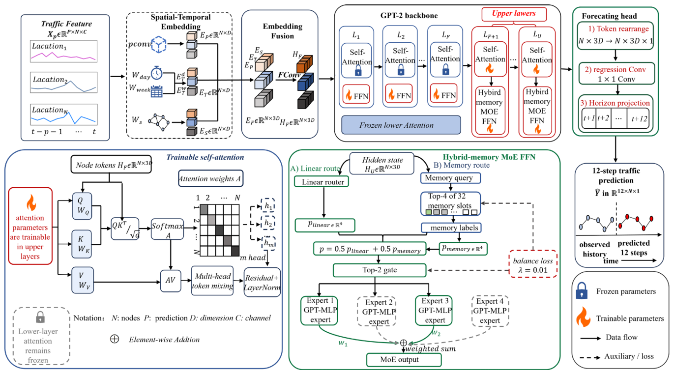
Figure 2.
Horizon-wise MAE comparison between FAMoE-ST and representative baselines on PEMS04 and PEMS08. Lower values indicate better performance.
Figure 2.
Horizon-wise MAE comparison between FAMoE-ST and representative baselines on PEMS04 and PEMS08. Lower values indicate better performance.
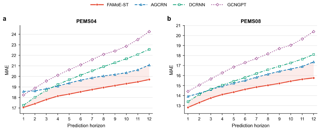
Figure 3.
Horizon-12 traffic-flow predictions of FAMoE-ST, AGCRN, and DCRNN on PEMS04 and PEMS08. Dashed rectangles identify the intervals reproduced in the right-hand local views.
Figure 3.
Horizon-12 traffic-flow predictions of FAMoE-ST, AGCRN, and DCRNN on PEMS04 and PEMS08. Dashed rectangles identify the intervals reproduced in the right-hand local views.
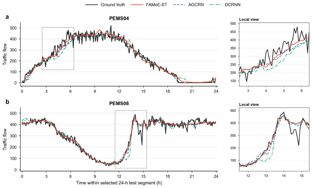
Figure 4.
Prediction consistency and sensitivity to the training-data ratio for FAMoE-ST.
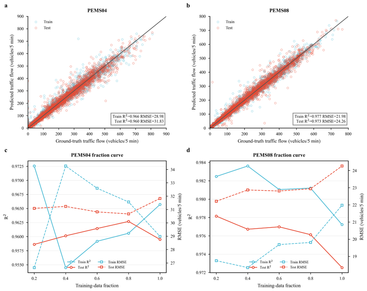
Figure 5.
Error changes after removing individual components, relative to the complete FAMoE-ST model.
Figure 5.
Error changes after removing individual components, relative to the complete FAMoE-ST model.
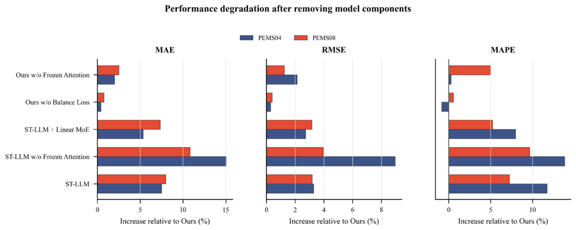
Figure 6.
Hybrid-memory mixture-of-experts routing diagnostics on PEMS04 and PEMS08. * The original linear-branch probability of Expert 1 on PEMS08 is 0.0003; a display floor of 0.02 is used for visibility, while all statistics are computed from the original value.
Figure 6.
Hybrid-memory mixture-of-experts routing diagnostics on PEMS04 and PEMS08. * The original linear-branch probability of Expert 1 on PEMS08 is 0.0003; a display floor of 0.02 is used for visibility, while all statistics are computed from the original value.
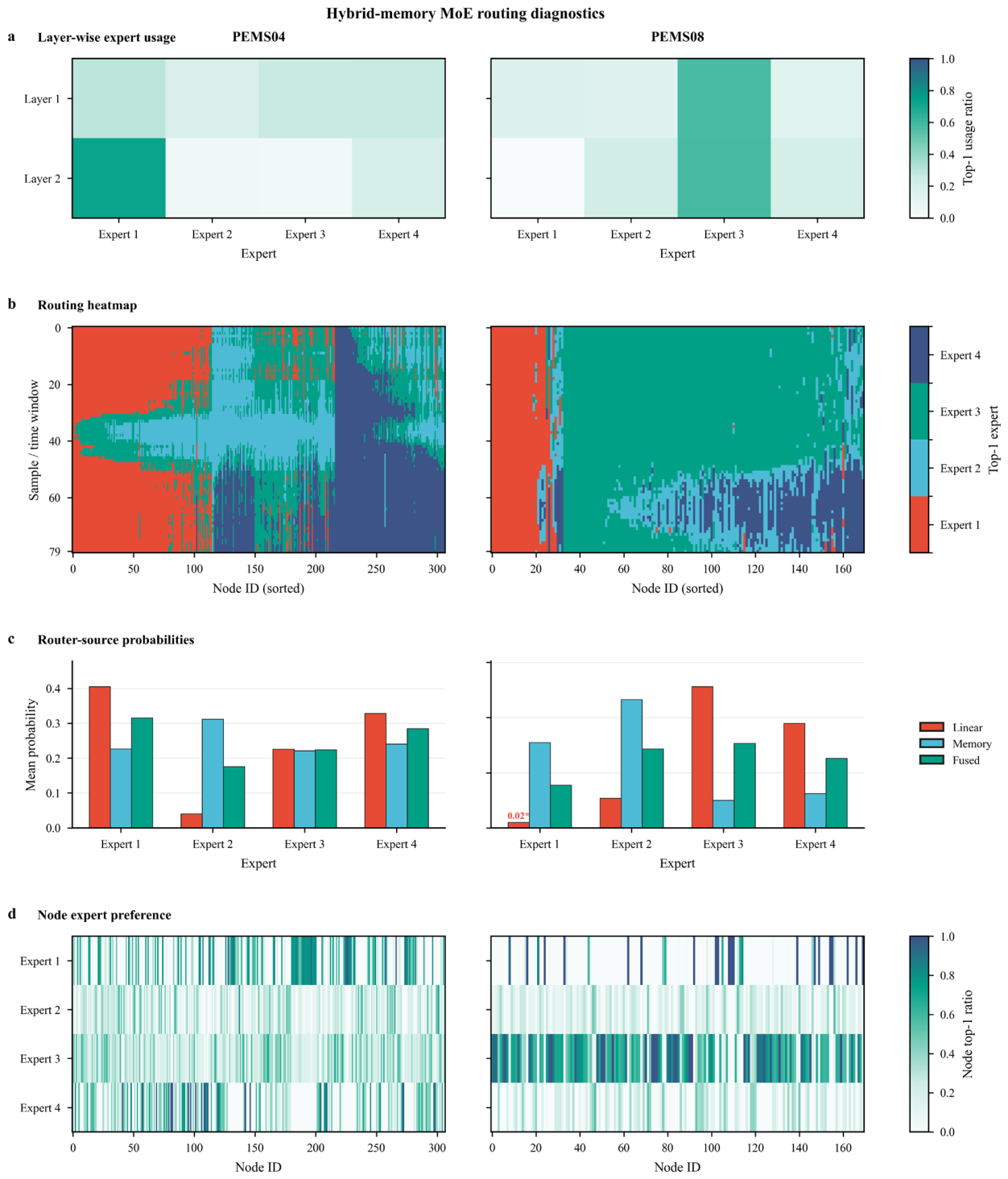

Table 1.
Dataset statistics.
| Dataset | Period | Nodes | Time Steps | Sampling Interval |
| PEMS04 | 2018.01-2018.02 | 307 | 16 992 | 5 min |
| PEMS08 | 2016.07-2016.08 | 170 | 17 856 | 5 min |
Table 2.
Forecasting performance on PEMS04 and PEMS08. Lower values indicate better performance; bold and underlined entries denote the best and second-best results, respectively.
Table 2.
Forecasting performance on PEMS04 and PEMS08. Lower values indicate better performance; bold and underlined entries denote the best and second-best results, respectively.
| Dataset | Model | Horizon 3 | Horizon 6 | Horizon 12 | 12-Step Average | ||||||||
| MAE | RMSE | MAPE | MAE | RMSE | MAPE | MAE | RMSE | MAPE | MAE | RMSE | MAPE | ||
| PEMS04 | GWN | 18.38 | 29.38 | 12.65% | 19.35 | 30.82 | 13.33% | 21.17 | 33.34 | 14.83% | 19.43 | 30.91 | 13.45% |
| MTGNN | 19.60 | 30.59 | 13.91% | 20.98 | 32.50 | 15.10% | 23.49 | 35.89 | 18.01% | 21.05 | 32.57 | 15.40% | |
| AGCRN | 18.82 | 30.95 | 12.53% | 19.64 | 32.29 | 12.89% | 21.08 | 34.63 | 13.93% | 19.69 | 32.41 | 13.01% | |
| DCRNN | 18.67 | 29.83 | 12.41% | 20.11 | 31.84 | 13.41% | 22.57 | 35.05 | 15.29% | 20.17 | 31.85 | 13.51% | |
| GATGPT | 18.91 | 29.80 | 13.25% | 20.23 | 31.60 | 14.34% | 22.64 | 34.71 | 17.51% | 20.34 | 31.68 | 14.71% | |
| GCNGPT | 19.56 | 30.66 | 13.39% | 21.09 | 32.80 | 15.01% | 24.26 | 36.83 | 18.84% | 21.27 | 32.93 | 15.27% | |
| StemGNN | 19.48 | 30.74 | 13.84% | 21.40 | 33.46 | 15.85% | 24.90 | 38.29 | 19.50% | 21.61 | 33.80 | 16.10% | |
| STGCN | 18.74 | 29.84 | 14.42% | 19.64 | 31.34 | 13.27% | 21.12 | 33.53 | 14.22% | 19.63 | 32.32 | 13.32% | |
| GMAN | 18.27 | 29.35 | 12.66% | 18.81 | 30.85 | 13.25% | 20.01 | 31.32 | 13.40% | 18.83 | 30.93 | 13.21% | |
| STNorm | 18.28 | 29.70 | 12.28% | 18.92 | 31.12 | 12.71% | 20.20 | 32.91 | 13.43% | 18.96 | 30.98 | 12.69% | |
| FAMoE-ST | 17.80 | 29.10 | 12.32% | 18.54 | 30.50 | 12.70% | 19.70 | 32.17 | 13.92% | 18.55 | 30.35 | 12.91% | |
| PEMS08 | GWN | 14.06 | 22.20 | 9.19% | 14.98 | 24.29 | 9.66% | 16.48 | 26.23 | 10.55% | 15.00 | 23.69 | 9.80% |
| MTGNN | 15.45 | 23.76 | 11.18% | 16.49 | 25.55 | 12.18% | 18.41 | 28.30 | 15.41% | 16.50 | 25.43 | 12.55% | |
| AGCRN | 14.60 | 23.02 | 9.46% | 15.50 | 24.74 | 10.05% | 17.36 | 27.58 | 11.25% | 15.64 | 24.90 | 10.16% | |
| DCRNN | 14.64 | 22.67 | 10.51% | 15.80 | 24.84 | 11.02% | 18.11 | 28.43 | 12.50% | 15.93 | 24.91 | 11.18% | |
| GATGPT | 15.35 | 23.57 | 10.29% | 16.71 | 25.82 | 11.19% | 19.30 | 29.62 | 12.66% | 16.84 | 25.89 | 11.18% | |
| GCNGPT | 15.66 | 23.94 | 10.40% | 17.29 | 26.54 | 11.11% | 20.39 | 30.76 | 13.49% | 17.43 | 26.56 | 11.56% | |
| StemGNN | 14.49 | 23.02 | 9.73% | 15.84 | 25.38 | 10.78% | 18.10 | 28.77 | 12.5% | 15.91 | 25.44 | 10.90% | |
| STGCN | 14.95 | 23.48 | 9.87% | 15.92 | 25.36 | 10.42% | 17.65 | 28.03 | 11.34% | 15.98 | 25.37 | 10.43% | |
| GMAN | 13.80 | 22.88 | 9.41% | 14.62 | 24.12 | 9.57% | 15.72 | 26.47 | 10.56% | 14.81 | 24.19 | 9.82% | |
| STNorm | 14.44 | 22.68 | 9.32% | 15.53 | 25.07 | 9.98% | 17.20 | 27.86 | 11.30% | 15.54 | 25.01 | 10.03% | |
| FAMoE-ST | 13.75 | 22.14 | 9.28% | 14.62 | 23.57 | 9.84% | 15.76 | 26.35 | 10.61% | 14.57 | 24.08 | 9.71% | |
Table 3.
Component ablation results for FAMoE-ST.
| Dataset | Model | Frozen Attention | MoE | Memory Routing/Balance Loss | 12-Step Average | ||
| MAE | RMSE | MAPE(%) | |||||
| PEMS04 | ST-LLM | Yes | No | No/No | 19.935 | 31.349 | 14.427 |
| ST-LLM (w/o Freezing) | No | No | No/No | 21.334 | 33.075 | 14.698 | |
| ST-LLM + Linear MoE | Yes | Yes | No/No | 19.534 | 31.181 | 13.943 | |
| FAMoE-ST (w/o Balance Loss) | Yes | Yes | Yes/No | 18.621 | 30.441 | 12.804 | |
| FAMoE-ST (w/o Freezing) | No | Yes | Yes/Yes | 18.916 | 31.000 | 12.947 | |
| FAMoE-ST (Full) | Yes | Yes | Yes/Yes | 18.545 | 30.353 | 12.914 | |
| PEMS08 | ST-LLM | Yes | No | No/No | 15.733 | 24.849 | 10.414 |
| ST-LLM (w/o Freezing) | No | No | No/No | 16.145 | 25.037 | 10.647 | |
| ST-LLM + Linear MoE | Yes | Yes | No/No | 15.640 | 24.843 | 10.218 | |
| FAMoE-ST (w/o Balance Loss) | Yes | Yes | Yes/No | 14.682 | 24.180 | 9.764 | |
| FAMoE-ST (w/o Freezing) | No | Yes | Yes/Yes | 14.937 | 24.383 | 10.194 | |
| FAMoE-ST (Full) | Yes | Yes | Yes/Yes | 14.570 | 24.083 | 9.710 | |
Table 4.
Capacity-matched comparison on PEMS04. MACs denote theoretical FFN-and-router multiply-accumulate operations per token in each modified layer; lower values are better.
Table 4.
Capacity-matched comparison on PEMS04. MACs denote theoretical FFN-and-router multiply-accumulate operations per token in each modified layer; lower values are better.
| Variant | Total Params (M) | Trainable Params (M) | MACs/Token/Layer (M) | MAE | RMSE | MAPE (%) |
| Parameter-matched Dense FFN | 112.245 | 44.522 | 19.493 | 19.176 | 31.680 | 13.101 |
| Hybrid-memory MoE | 112.246 | 44.523 | 10.055 | 18.728 | 30.644 | 12.732 |
Table 5.
Empirical efficiency of the capacity-matched variants on an NVIDIA GeForce RTX 4060 Ti. F+B denotes one forward-and-backward pass; batch size is 4. Values are means over 20 measured iterations after five warm-up iterations.
Table 5.
Empirical efficiency of the capacity-matched variants on an NVIDIA GeForce RTX 4060 Ti. F+B denotes one forward-and-backward pass; batch size is 4. Values are means over 20 measured iterations after five warm-up iterations.
| Variant | F+B Time (ms) | Train Peak (MiB) | Epoch Time (s) | Batch Latency (ms) | Throughput (samples/s) | Single Latency (ms) |
| Parameter-matched Dense FFN | 86.37 | 2524.33 | 278.82 | 32.11 | 124.57 | 8.03 |
| Hybrid-memory MoE | 69.94 | 2102.40 | 204.25 | 26.35 | 151.81 | 13.16 |
Disclaimer/Publisher’s Note: The statements, opinions and data contained in all publications are solely those of the individual author(s) and contributor(s) and not of MDPI and/or the editor(s). MDPI and/or the editor(s) disclaim responsibility for any injury to people or property resulting from any ideas, methods, instructions or products referred to in the content. |
© 2026 by the authors. Licensee MDPI, Basel, Switzerland. This article is an open access article distributed under the terms and conditions of the Creative Commons Attribution (CC BY) license.
Copyright: This open access article is published under a Creative Commons CC BY 4.0 license, which permit the free download, distribution, and reuse, provided that the author and preprint are cited in any reuse.