

Submitted:
06 August 2026
Posted:
06 August 2026
You are already at the latest version
Abstract
Bigeye tuna (Thunnus obesus) are ecologically important pelagic predators in the eastern Pacific and support valuable international fisheries. Their distribution responds sensitively to the El Niño–Southern Oscillation (ENSO) and to multiscale changes in upper‑ocean structure. However, existing statistical or machine‑learning models often fail to distinguish between environmental suitability and advective redistribution, while complex ecosystem models often face parameter identifiability challenges. To bridge this gap we develop a Physics‑Guided Advection‑Diffusion‑Reaction (PhyG‑ADR) model. The model represents the time‑varying biomass density C(x,y,t) by a partial differential equation where advection describes large‑scale movement, diffusion represents mixing and sub‑mesoscale dispersion, and the reaction term implements environment‑dependent growth and density limitation. A non‑linear habitat selection function combines sea‑surface temperature, mixed‑layer depth, dissolved oxygen, and ocean‑heat content to provide physiological realism. To constrain poorly known parameters, we used a Bayesian inference framework and estimated posterior parameter distributions from a 19-year record of monthly catch-per-unit-effort (CPUE) indices (1994–2012) using Markov chain Monte Carlo (MCMC). The posterior analysis suggests that habitat selection dominates the formation of spatial aggregation, while climate‑driven advection plays a key role in inter‑annual shifts associated with ENSO. Parameter uncertainty is explicitly quantified, and sensitivity experiments demonstrate that the inferred habitat-preference structure of bigeye tuna is robust across carrying‑capacity scenarios. PhyG‑ADR therefore combines predictive skill with mechanistic insight and can inform dynamic fisheries management and spatial conservation planning.
Keywords:
bigeye tuna
; partial differential equation
; advection–diffusion–reaction model
; MCMC parameter assimilation
; ENSO
1. Introduction
Bigeye tuna (Thunnus obesus) are a major pelagic predator in the Pacific Ocean and support one of the world's most valuable fisheries [1,2]. As highly migratory species, their spatiotemporal distribution is exquisitely sensitive to marine environmental gradients and large-scale climate variability [3,4,5]. In particular, the El Niño-Southern Oscillation (ENSO) periodically reshapes the thermal structure, ocean circulation, and primary productivity of the Pacific Ocean, triggering profound reorganizations of pelagic habitats [6,7,8]. For instance, the zonal displacement of the western Pacific warm pool during El Niño events directly drives the large-scale eastward migration of tuna populations [8,9]. Therefore, understanding and accurately predicting the distribution dynamics of bigeye tuna under climate forcing is crucial for sustainable fisheries management and dynamic spatial conservation [10,11,12].
Despite the well-documented impacts of climate on marine ecosystems, accurately simulating tuna distribution remains challenging due to the complex interplay between physiological constraints and the three-dimensional marine environment. Previous habitat studies have primarily focused on sea surface temperature (SST) and dissolved oxygen to define the physiological boundaries of tunas [3,13,14,15]. However, these simplified environmental indicators often fail to capture the habitat compression or expansion experienced by pelagic fish. Cold, hypoxic subsurface layers can compress the vertical habitat available to high-performance tropical pelagic fishes [40]. Bigeye tuna exhibit pronounced deep foraging behaviors, making their distribution highly dependent on the upper ocean's thermal structure, specifically the mixed layer depth (MLD) and ocean heat content (OHC) [4,13,14,16]. The MLD determines the vertical accessibility of the deep scattering layer, while the OHC integrates the thermodynamic state of the water column, acting as a critical energy reservoir during climate anomalies. Relying solely on a limited set of environmental variables overlooks the synergistic constraints of the 3D marine environment, creating a critical limitation in current habitat suitability assessments.
Beyond static environmental suitability, the spatial dynamics of highly migratory species are fundamentally governed by ocean physical transport, yet these processes are frequently isolated from habitat selection in existing models. Population movement is driven by both large-scale advection from ocean currents and effective diffusion representing unresolved mesoscale and submesoscale mixing and dispersal [17,18]. While climate-driven velocity fields force the directed migration of populations, mesoscale eddies create highly heterogeneous diffusion pathways, effectively trapping nutrients and aggregating prey to form localized hotspots [16,19,20]. However, traditional spatial models often treat physical transport and biological habitat preference as independent modules or oversimplify diffusion as uniform random walks. This artificial separation obscures how climate anomalies simultaneously alter passive physical dispersal and active biological aggregation, limiting the ability to mechanistically explain distribution shifts under extreme ENSO events.
Methodologically, current modeling frameworks struggle to reconcile mechanistic physical-ecological processes with the statistical rigor required to assimilate rich observational data. Pure data-driven statistical models (e.g., machine learning) excel at fitting historical abundance patterns but often have limited mechanistic interpretability. They often conflate density-dependent population regulation with environmental adaptation, which can lead to false "niche drift" predictions under future climate scenarios [21,22,23,24]. Conversely, complex mechanistic ecosystem models provide comprehensive physiological descriptions but suffer from limited parameterization capacity and high computational barriers [16,19,20]. There is an urgent need for an intermediate-complexity framework that couples environment-dependent habitat selection with heterogeneous physical transport, while remaining computationally tractable for rigorous data assimilation.
To address these critical gaps, this study proposes a Physics-Guided Advection-Diffusion-Reaction (PhyG-ADR) modeling framework tailored for bigeye tuna in the eastern Pacific. By embedding a multi-factor non-linear habitat selection function into a partial differential equation, the PhyG-ADR model explicitly couples ocean physical transport with density-dependent ecological responses. Furthermore, we leverage Bayesian parameter inference to integrate long-term fisheries observations, directly estimating the key dynamical parameters governing advection, diffusion, and environmental preference. Specifically, this study aims to answer the following core scientific questions: (1) How do upper-ocean environmental structure and physical transport processes synergistically drive the spatial distribution of bigeye tuna? (2) What is the relative contribution of habitat selection versus advection-diffusion during extreme ENSO events? (3) Can the PhyG-ADR framework successfully decouple the species' fundamental habitat preference structure from density-dependent population fluctuations? By answering these questions, this research provides a robust, interpretable tool for assessing the climate adaptability of pelagic fisheries and supporting dynamic ocean management.
2. Materials and Methods
2.1. Data Sources and Preprocessing
We assembled a spatio-temporal database covering the eastern Pacific Ocean (EPO), with a focus on the eastern equatorial region. The study period (1994–2012) spans multiple ENSO warm and cold events and matches the period analyzed by Lian and Gao [4] for comparability. Monthly catch-per-unit effort (CPUE) indices for bigeye tuna were obtained from the Inter-American Tropical Tuna Commission (IATTC)[4]. Only high-quality records with unambiguous spatial and temporal tags were retained. Observations were subjected to standard quality control (removal of duplicates and outliers, unit harmonization, and geolocation checks) and aggregated by month on a 1° × 1° latitude–longitude grid. CPUE reflects relative abundance but is influenced by fishing effort and targeting behavior; aggregation mitigates sampling irregularity, and no spatial interpolation was applied to the fishery observations in order to avoid generating artificial data. The resulting dataset contains approximately 60,000 monthly grid-cell observations of CPUE.
Environmental drivers were assembled from multiple sources to characterize the thermal, dynamic, biogeochemical, and topographic conditions of bigeye tuna habitat. The candidate predictor set included sea-surface temperature (SST), wind speed, mixed-layer depth (MLD), sea-surface height (SSH), chlorophyll-a concentration (CHL-a), ocean heat content (OHC), dissolved oxygen (O2), bathymetry, and marine heatwaves (MHWs) (Fig. 1) . MHWs were identified from daily NOAA OISST v2.1 using a seasonally varying 90th-percentile threshold calculated over the 1982–2011 baseline period. Events lasting at least five consecutive days were retained, and events separated by gaps of no more than two days were merged. Here we used mean intensity to represent the index of HMWs.
SST fields were taken from NOAA’s Optimum Interpolation SST version 2, a global 0.25° daily dataset that merges satellite and in-situ observations. SSH and related surface dynamic conditions were obtained from AVISO/CMEMS multi-mission altimetry. Mixed-layer depth and ocean-heat content, defined as the vertically integrated heat content above the 26 °C isotherm, were taken from NOAA upper-ocean temperature analyses. Dissolved oxygen fields relevant to subsurface habitat conditions were derived from climatological and reanalysis products. Chlorophyll-a was used as a proxy for lower-trophic productivity, bathymetry described large-scale topographic structure, and marine heatwaves were used to characterize extreme thermal anomalies. All environmental variables were averaged to monthly means and regridded to the 1° × 1° grid(Figure 1). To focus on interannual variability, linear trends associated with long-term warming were removed from SST, OHC, and SSH-related fields. We applied identical land-sea masks and carefully treated coastal and boundary cells to avoid artefacts. Unlike the environmental data, CPUE observations were not spatially interpolated; each grid cell retains only real observations.
2.2. Model Formulation
We established a partial differential equation model for the mechanic distribution of tuna species in Pacific Ocean (Figure 2). And we simulated the biomass density C(x,y,t) using an advection–diffusion–reaction equation:
where u(x,y,t) is the advection velocity field, D(x,y,t) is an effective diffusion coefficient, and R(C, E) is a reaction term representing local growth and mortality as a function of biomass and environmental variables E [17,18,25]. The model is solved on the monthly 1° grid using an explicit finite-difference scheme with appropriate boundary conditions (zero-flux at land boundaries and open boundaries at 100°E and 290°E). A monthly time step is used, consistent with the temporal resolution of the observations.
2.2.1. Advection Velocity
Directed movement is represented by an advection term . A purely geostrophic velocity would not capture behavioural responses to climate anomalies; we therefore augment the baseline geostrophic field with a climate-driven component estimated from the migration of the population centre of gravity (COG). At each month, the COG of observed biomass is computed as :
The difference between consecutive COGs defines a displacement vector, and the climate-driven velocity is obtained by dividing by the monthly time step . The total velocity is then defined as:
where is the background geostrophic velocity and is a tunable scaling parameter estimated by Bayesian assimilation. This approach allows the model to follow ENSO-driven zonal shifts evident in the CPUE record.
2.2.2. Diffusion
Small-scale mixing and the aggregated effect of unresolved behaviors are represented by an effective diffusion coefficient:
where is a baseline diffusivity and scales the influence of mesoscale eddies represented by the magnitude of the SSH gradient. The use of eddy-enhanced diffusion reflects observations that tuna aggregations are influenced by fronts and eddies. Both parameters are estimated using the MCMC framework.
2.2.3. Reaction Term and Habitat Suitability
Local population dynamics combine density-dependent growth and environmental carrying capacity. We use a logistic structure in which the intrinsic growth rate r(E) and carrying capacity K(E) depend on environmental drivers and are separated to avoid parameter confounding. The reaction term takes the form
where γ represents a background loss rate that includes natural mortality and unmodelled processes. Density dependence becomes important as approaches K(E), while r(E) controls growth when abundance is low. This formulation is analogous to the Schaefer logistic model, in which the intrinsic growth rate r and carrying capacity K set the production curve and density-dependent term. In the continuous version the density-dependent term appears in the reaction term rather than as a discrete difference[25].
The intrinsic growth rate r(E) reflects the physiological effects of temperature and oxygen. We define:
where α is the maximum growth rate. is a Gaussian thermal response centred on the optimum temperature with width , which reflects the unimodal thermal niche of bigeye tuna[13]; metabolic rates and swimming capacity decline when the environment deviates from the optimum. , is a Michaelis–Menten saturation function of dissolved oxygen:
while half-saturation constant . Michaelis–Menten functions are widely used to represent biological rates that saturate at high substrate levels. This formulation ensures that growth decreases under hypoxic conditions but approaches α when oxygen is plentiful [13,25].
Habitat suitability S(E) integrates multiple environmental factors to determine the carrying capacity K(E). Following niche theory, we assume that suitability is multiplicative and declines if any factor departs from its preferred range[21,22]. The suitability function comprises four non-linear responses:
where is the same Gaussian thermal response used in r(E), and are logistic functions of mixed-layer depth and ocean-heat content, and is the Michaelis–Menten oxygen term. Logistic functions represent threshold-like responses that saturate beyond certain values. Bigeye tuna tend to prefer shallow mixed layers that facilitate vertical foraging and avoid very deep thermoclines[4,13,14]; logistic functions capture this tendency. Ocean-heat content reflects the integrated thermal energy available in the water column and influences food availability and habitat volume. Using these functions allows the model to allocate carrying capacity to regions with suitable thermal, structural and oxygen conditions. The carrying capacity is then expressed as K(E) = K0× S(E) × [1 + δ P(E)], where K0 is a baseline capacity and δ P(E) accounts for productivity enhancements when energy reserves (e.g. primary production) are high.
2.3. Parameter Assimilation via Mcmc
Twelve parameters θ = {D0, D1,, α, δ, γ, , , , , } control the advection, diffusion and reaction terms. To estimate them and quantify uncertainty we adopt a Bayesian framework[26,27,28]. A likelihood function is defined by comparing simulated biomass C(x,y,t) integrated over each grid cell with the observed abundance after appropriate scaling:
We assume additive Gaussian observation errors with variance . Uniformly informative priors are assigned to each parameter based on physiology and literature values. Posterior samples of are obtained using the affine-invariant ensemble MCMC (Figure 3) sampler of Goodman and Weare [29], implemented using emcee [30]. This algorithm runs multiple chains in parallel and adapts the proposal distribution to improve sampling efficiency. Each chain consists of 10 000 iterations with a burn-in of 5 000 to allow convergence. Convergence diagnostics include trace plots, effective sample size calculations, and the Gelman–Rubin statistic, which compares variance within and between chains; values near 1 indicate convergence [31]. We also monitor the acceptance ratio and adapt the proposal width to maintain it between 0.2 and 0.5. Parameter posterior means and credible intervals are used in subsequent analyses.
3. Results
The PhyG-ADR model reproduces the observed spatio-temporal variability of bigeye tuna abundance in the eastern Pacific. Hindcasts over 1994–2010 show spatial root-mean-square error reductions of 2.4% compared with benchmark statistical models including the Generalized Additive Model (GAM) [32], Support Vector Regression (SVR) [33], and XGBoost [34] (Table 1). Further performance differences are illustrated using a Taylor Diagram [35] (Figure 4), which demonstrates that PhyG-ADR achieves the highest spatial-temporal correlation and successfully captures the true amplitude of variability (normalized standard deviation near 1.0), enabling skillful prediction of the timing of biomass peaks and troughs associated with ENSO warm and cold phases.
Spatial comparison of the observed and model-predicted mean bigeye tuna CPUE in the eastern Pacific Ocean during 1994–2012(Figure 5). The left column shows the observed mean CPUE fields repeated for row-wise comparison [(a), (d), (g), and (j)]. The middle column presents the corresponding predictions from (b) PhyG-ADR, (e) XGBoost, (h) support vector regression (SVR), and (k) generalized additive model (GAM). The right column shows the prediction residuals, calculated as predicted minus observed CPUE, for (c) PhyG-ADR, (f) XGBoost, (i) SVR, and (l) GAM. Positive residuals indicate model overestimation, whereas negative residuals indicate underestimation. Observed and predicted fields share the same CPUE color scale, and residual maps use a common diverging color scale. RMSE values were calculated over grid cells with valid observations. Land areas are shown in gray.
Consistent with the overall performance metrics reported in Table 1, the spatial comparison further showed that PhyG-ADR provided the closest reconstruction of the observed mean CPUE distribution (Figure 5). All four models reproduced the broad zonal distribution of bigeye tuna CPUE across the eastern Pacific Ocean, including the equatorial high-CPUE band and the large-scale meridional gradient. However, their ability to represent regional-scale spatial variability differed substantially. PhyG-ADR achieved the lowest RMSE (0.0886), followed by XGBoost (0.0908), SVR (0.0993), and GAM (0.1164). Thus, the reduction in RMSE achieved by PhyG-ADR was approximately 2.4% relative to XGBoost, 10.8% relative to SVR, and 23.9% relative to GAM. The relatively small difference between PhyG-ADR and XGBoost indicates that their overall predictive accuracy was similar, although PhyG-ADR produced more spatially localized residuals and better retained the observed zonal structure. The PhyG-ADR residuals were generally centered around zero across most of the study domain, with larger errors confined primarily to localized boundary and coastal regions. XGBoost reproduced the broad spatial pattern but showed more spatially scattered positive and negative residuals. SVR exhibited more extensive negative residuals in the central and southern portions of the study area, indicating systematic underestimation in these regions. GAM generated an overly smooth spatial field and failed to reproduce several finer-scale features apparent in the observations. These results suggest that the process-based constraints incorporated into PhyG-ADR improved the representation of spatial structure, although its numerical advantage over XGBoost remained modest.
Through Bayesian parameter assimilation (Figure 3), posterior estimates indicate that the climate-driven advection coefficient is 0.6 ± 0.1 (95 % credible interval), implying that population movement follows about 60 % of the COG displacement, while the eddy-enhanced diffusion coefficient D1 is significantly positive, confirming the role of fronts in mixing biomass. The intrinsic growth rate α is estimated at 0.25 month⁻¹ (0.18–0.32 month⁻¹) and the optimum temperature at 25.5 °C (24.8–26.2 °C), consistent with physiological observations that bigeye tuna thrive between 24 °C and 28 °C. The half-saturation constant for oxygen is 2.8 mL L⁻¹, indicating strong suppression of growth under hypoxic conditions. The posterior distribution of the MLD-response midpoint, Hopt was concentrated around 57 m, indicating that the modeled influence of mixed-layer depth changed most rapidly near this depth. The posterior distribution of KMLD was comparatively broad, suggesting residual uncertainty in the steepness of the MLD response. The OHC-response coefficient KOHC was centered near −0.07; under the specified sign convention, this negative coefficient indicates a decreasing modeled response with increasing OHC. These parameters describe associations within the habitat-capacity formulation and should not be interpreted as experimentally determined physiological thresholds (Figure 3).
Mechanistic analysis reveals that habitat selection is the dominant driver of spatial aggregation. When the habitat suitability function S(E) is disabled (by replacing it with a constant), the model underestimates the high-abundance zones and overestimates diffuse distributions. In contrast, removing the climate-driven advection component results in poor representation of east–west shifts during El Niño and La Niña events. During the strong 1997/98 and 2009/10 El Niño events, advection accounted for more than 50% of the model-attributed variance in spatial redistribution, whereas the habitat-related reaction component accounted for more than 70% during ENSO-neutral periods. Sensitivity experiments in which the baseline carrying capacity K₀and productivity scaling δ are varied by ±50 % show that the optimum temperature and oxygen thresholds remain within the posterior credible intervals, demonstrating the robustness of the estimated fundamental thermal niche to changes in carrying capacity (Figure 6). The relative contribution of the modeled processes varied among climate states, with advection becoming more influential during strong El Niño events and habitat-related processes contributing more strongly during ENSO-neutral periods.
At the basin-aggregated scale, the monthly mean relative-abundance index reconstructed by PhyG-ADR broadly followed the temporal evolution of the observed series during 1994–2012 (Figure 7). The model reproduced several major declines and subsequent recoveries, including the pronounced decrease around 2005–2006, indicating that it captured a substantial component of the low-frequency variability in the observations. However, the simulated series generally exhibited a smaller amplitude than the observed series: several short-lived maxima were underestimated, whereas some abrupt minima were only partially reproduced. This temporal smoothing suggests that the monthly 1° process-based model represents broad inter-annual changes more effectively than high-frequency fluctuations, which may additionally reflect short-term fish movement, heterogeneous fishing effort, catchability variation, and observation error. Although some reconstructed changes coincided with major ENSO periods, Figure 7 alone does not establish an ENSO-driven response; such attribution requires an explicit comparison with an ENSO index and event-based statistical evaluation.
4. Discussion
4.1. Physical Interpretability and Ecological Insights
The PhyG-ADR model advances fisheries oceanography by bridging the gap between physical oceanography and ecological modeling in a parsimonious but mechanistically explicit framework. Compared with purely statistical habitat models, it provides robust insights into the relative roles of habitat preference and physical movement in shaping fish distribution, and can therefore be more confidently extrapolated to novel climate states [23,24,36]. The dominance of habitat selection in our posterior analysis is consistent with the view that bigeye tuna maintain a relatively conservative thermal niche, as suggested by growth and metabolic studies [13]. While habitat selection dominates the overall distribution pattern, the inclusion of climate-driven advection is critical to reproduce the large-scale east–west shifts associated with ENSO [4,8,9]. The estimated optimum temperature () and half-saturation oxygen threshold () align with laboratory-derived tolerance ranges, supporting the ecological validity of the model [13]. Furthermore, the eddy-enhanced diffusion term underscores the importance of fronts and mesoscale structures in fish aggregation [16,19,20]. This finding highlights the necessity of explicitly representing such physical oceanographic features, as done in PhyG-ADR, to inform dynamic fisheries management tools [10,11,12].
4.2. Parameter Assimilation and Mechanism Robustness
The Bayesian assimilation framework provides a rigorous quantification of parameter uncertainty and addresses identifiability issues that have hampered previous mechanistic models. Convergence diagnostics (such as MCMC trace plots and the Gelman–Rubin statistic, shown in Figure 3) indicate well-behaved posterior sampling [27,28,29,30,31]. However, some parameters, such as the productivity scaling factor , remain weakly constrained in the current setup, as CPUE data primarily reflects relative abundance and provides limited direct information on bottom-up trophic dynamics. Future work could incorporate independent estimates of primary production or prey density to reduce parameter equifinality. Specifically, prey density data would help disentangle the complex effects of temperature and food availability on habitat selection, thereby better constraining and the baseline carrying capacity .
4.3. Implications for Management
As demonstrated by the model's ability to accurately track population shifts during ENSO events, static marine protected areas (MPAs) are insufficient for highly migratory species like bigeye tuna, whose distributions are tightly coupled to dynamic oceanographic conditions [2]. The successful parameterization of climate-driven advection and habitat suitability provides a robust basis for implementing Dynamic Ocean Management (DOM) [10,11,12]. By utilizing near real-time environmental monitoring and the predictive capabilities of the PhyG-ADR model, fisheries managers can dynamically adjust conservation boundaries to protect core habitats while minimizing disruptions to sustainable fishing operations.
4.4. Model Limitations and Implicit Vertical Representation
The use of a 1° grid and monthly time step in this study is a strategic choice to balance computational efficiency with macro-ecological spatial resolution, though it inherently neglects sub-monthly movements and explicit vertical behavior (e.g., diel vertical migration). Nevertheless, the 2D horizontal framework implicitly integrates these processes by incorporating mixed-layer depth (MLD) and ocean heat content (OHC) as proxy covariates in the habitat suitability function. These proxies successfully capture key vertical habitat constraints without requiring full 3D modeling. This limitation is particularly important because ocean deoxygenation and expanding oxygen-minimum zones can reduce the vertical habitat available to pelagic fishes [37,38,39]. The spatially localized residuals of PhyG-ADR, particularly relative to the smoother GAM reconstruction, indicate an improved representation of regional distributional heterogeneity (Figure 5). Extending the model to three dimensions with depth-resolved habitat functions and incorporating fishing effort dynamics would further improve ecological realism. Finally, PhyG-ADR offers a valuable middle ground between purely statistical models and fully coupled, highly complex ecosystem models such as SEAPODYM [16,19,20]. While it significantly reduces the parameter space compared with complex ecosystem counterparts, its mechanistic complexity still increases computational cost. The GPU-accelerated solver and ensemble MCMC used here mitigate this issue, but scalability remains a challenge for global, high-resolution applications.
5. Conclusions
This study developed and evaluated a physics-guided advection–diffusion–reaction model with Bayesian parameter assimilation (PhyG-ADR) to reconstruct the monthly distribution of bigeye tuna in the eastern tropical Pacific during 1994–2012. By integrating environmental suitability, effective transport, diffusion, and density-dependent regulation within a unified partial differential equation framework, the model provides a process-informed alternative to purely empirical approaches. PhyG-ADR achieved the lowest prediction error (RMSE=0.0886), compared with XGBoost (0.0908), SVR (0.0993), and GAM (0.1164). Although its improvement over XGBoost was modest, the model better retained the observed large-scale spatial structure and produced more localized residuals. Bayesian inference yielded ecologically interpretable environmental-response parameters, including an estimated optimum sea surface temperature of approximately 27.26 °C. This estimate should be interpreted as the modeled thermal response of fisheries-dependent relative abundance rather than as a direct measurement of the species’ fundamental physiological niche. The ablation experiments further indicated that removing the habitat-selection component caused the greatest deterioration in the reconstructed spatial aggregation pattern, whereas removing the advective component primarily reduced the model’s ability to reproduce ENSO-associated zonal redistribution. Sensitivity experiments showed that changes in relative carrying capacity substantially affected the magnitude of predicted abundance but had less influence on the normalized shape of the thermal-response curve. These findings suggest that environmental suitability and transport play complementary roles in shaping the mean distribution and climate-related redistribution of bigeye tuna within the model framework.
PhyG-ADR therefore provides a potentially useful framework for dynamic habitat assessment and short-term distribution forecasting. However, the present results are based on fisheries-dependent CPUE and a two-dimensional representation that does not explicitly resolve catchability variation, diel vertical migration, subsurface thermal and oxygen structure, prey availability, fishing behavior, or life-history differences. Accordingly, the inferred processes should not be interpreted as definitive causal mechanisms or direct estimates of absolute biomass. Future work should incorporate standardized fishery indices, tagging or fishery-independent observations, depth-resolved environmental fields, and explicitly modeled fishing effort. Independent spatiotemporal validation, particularly during withheld ENSO and marine heatwave events, will also be necessary before the framework can be applied operationally to dynamic fisheries management and marine spatial planning.
Author Contributions
Conceptualization, Y.M., Y.W. and P.L.; methodology, Y.W.,Z. Z. and P.L.; validation, Y.M., Y.W. and P.L.; formal analysis, Y.M., Y.W. and P.L.; investigation, Y.M., R.Z., G.Z. and W.Y.; resources, P.L.; data curation, Y.M., R.Z. and W.Y.; writing—original draft preparation, Y.M. and Y.W.; writing—review and editing, P.L., R.Z., G.Z. and W.Y.; visualization, Y.M. and Y.W.; supervision, P.L.; project administration, P.L.; funding acquisition, P.L. All authors have read and agreed to the published version of the manuscript.
Funding
This research was funded by the Guangxi Key Laboratory of Beibu Gulf Marine Resources, Environment and Sustainable Development (MRESD-2024-B06), the National Marine Satellite Application Center Key Laboratory Open Fund (202402005), the Fund of Key Laboratory for Sustainable Utilization of Open-Sea Fishery, Ministry of Agriculture and Rural Affairs (LOF 2025-01), the Guangdong Provincial Key Laboratory of Fishery Ecology and Environment (FEEL-2025-07), the Fund of Key Laboratory of Marine Ranching, Ministry of Agriculture and Rural Affairs (KLMR-2024-2), the Aquatic Biodiversity and Watershed Environmental Protection Innovation Team Program, Chinese Academy of Fishery Sciences (2023TD12), the Central Public-interest Scientific Institution Basal Research Fund, Chinese Academy of Fishery Sciences (2024A005, 2025YJ01 and 2026XT1802), and the National Key Research and Development Program of China (2024YFD2401405). The APC was funded by the authors’ institutions.
Data Availability Statement
The public-domain purse-seine catch and effort data are available from the Inter-American Tropical Tuna Commission at https://www.iattc.org/en-US/Data/Public-domain. NOAA OISST data are available at https://www.ncei.noaa.gov/products/optimum-interpolation-sst. DUACS sea-level and geostrophic-current data and the global biogeochemical hindcast are available from the Copernicus Marine Data Store at https://data.marine.copernicus.eu/. NOAA mixed-layer-depth and ocean-heat-content products are available at https://www.ncei.noaa.gov/archive/accession/NESDIS-OHC. ERA5 data are available from the Copernicus Climate Data Store, and GEBCO bathymetry is available at https://www.gebco.net/.
Acknowledgments
The authors gratefully acknowledge the Inter-American Tropical Tuna Commission (IATTC) for providing the public-domain purse-seine catch and fishing-effort data for the eastern Pacific Ocean. The authors also acknowledge the National Oceanic and Atmospheric Administration (NOAA), including the National Centers for Environmental Information (NCEI) and the National Environmental Satellite, Data, and Information Service (NESDIS), for providing the Optimum Interpolation Sea Surface Temperature (OISST), mixed-layer-depth, and ocean-heat-content products. Sea-level anomaly, sea-surface height, geostrophic-current, and marine biogeochemical data were provided by the Copernicus Marine Service. And bathymetric data were obtained from the General Bathymetric Chart of the Oceans (GEBCO). The authors sincerely thank the institutions and data-processing teams responsible for producing, maintaining, and openly distributing these datasets.
Conflicts of Interest
The authors declare no conflicts of interest.
References
- FAO. The State of World Fisheries and Aquaculture 2022: Towards Blue Transformation; Food and Agriculture Organization of the United Nations: Rome, Italy, 2022. [Google Scholar] [CrossRef]
- Sibert, J.R.; Senina, I.; Lehodey, P.; Hampton, J. Shifting from marine reserves to maritime zoning for conservation of Pacific bigeye tuna (Thunnus obesus). Proc. Natl. Acad. Sci. USA 2012, 109, 18221–18225. [Google Scholar] [CrossRef] [PubMed]
- Arrizabalaga, H.; Dufour, F.; Kell, L.; Merino, G.; Ibaibarriaga, L.; Chust, G.; Irigoien, X.; Santiago, J.; Murua, H.; Fraile, I.; et al. Global habitat preferences of commercially valuable tuna. Deep Sea Res. Part II Top. Stud. Oceanogr. 2015, 113, 102–112. [Google Scholar] [CrossRef]
- Lian, P.; Gao, L. Impacts of central-Pacific El Niño and physical drivers on eastern Pacific bigeye tuna. J. Oceanol. Limnol. 2024, 42, 972–987. [Google Scholar] [CrossRef]
- Lian, P.; Gao, L. Contrasting physical mechanisms of yellowfin tuna fluctuations between the western and eastern Indian Ocean. J. Oceanol. Limnol. 2024, 42, 960–971. [Google Scholar] [CrossRef]
- Trenberth, K.E. The definition of El Niño. Bull. Am. Meteorol. Soc. 1997, 78, 2771–2778. [Google Scholar]
- Philander, S.G.H. El Niño, La Niña, and the Southern Oscillation; Academic Press: San Diego, CA, USA, 1990; Volume 46. [Google Scholar]
- Lehodey, P. The pelagic ecosystem of the tropical Pacific Ocean: Dynamic spatial modelling and biological consequences of ENSO. Prog. Oceanogr. 2001, 49, 439–468. [Google Scholar] [CrossRef]
- Lehodey, P.; Bertignac, M.; Hampton, J.; Lewis, A.; Picaut, J. El Niño Southern Oscillation and tuna in the western Pacific. Nature 1997, 389, 715–718. [Google Scholar] [CrossRef]
- Dunn, D.C.; Maxwell, S.M.; Boustany, A.M.; Halpin, P.N. Dynamic ocean management increases the efficiency and efficacy of fisheries management. Proc. Natl. Acad. Sci. USA 2016, 113, 668–673. [Google Scholar] [CrossRef] [PubMed]
- Maxwell, S.M.; Hazen, E.L.; Lewison, R.L.; Dunn, D.C.; Bailey, H.; Bograd, S.J.; Briscoe, D.K.; Fossette, S.; Hobday, A.J.; Bennett, M.; et al. Dynamic ocean management: Defining and conceptualizing real-time management of the ocean. Mar. Policy 2015, 58, 42–50. [Google Scholar] [CrossRef]
- Hazen, E.L.; Scales, K.L.; Maxwell, S.M.; Briscoe, D.K.; Welch, H.; Bograd, S.J.; Bailey, H.; Benson, S.R.; Eguchi, T.; Dewar, H.; et al. A dynamic ocean management tool to reduce bycatch and support sustainable fisheries. Sci. Adv. 2018, 4, eaar3001. [Google Scholar] [CrossRef] [PubMed]
- Brill, R.W. A review of temperature and oxygen tolerance studies of tunas pertinent to fisheries oceanography, movement models and stock assessments. Fish. Oceanogr. 1994, 3, 204–216. [Google Scholar] [CrossRef]
- Bigelow, K.A.; Hampton, J.; Miyabe, N. Application of a habitat-based model to estimate effective longline fishing effort and relative abundance of Pacific bigeye tuna (Thunnus obesus). Fish. Oceanogr. 2002, 11, 143–155. [Google Scholar] [CrossRef]
- Bertignac, M.; Lehodey, P.; Hampton, J. A spatial population dynamics simulation model of tropical tunas using a habitat index based on environmental parameters. Fish. Oceanogr. 1998, 7, 326–334. [Google Scholar] [CrossRef]
- Lehodey, P.; Senina, I.; Murtugudde, R. A spatial ecosystem and populations dynamics model (SEAPODYM)—Modeling of tuna and tuna-like populations. Prog. Oceanogr. 2008, 78, 304–318. [Google Scholar] [CrossRef]
- Sibert, J.R.; Hampton, J.; Fournier, D.A.; Bills, P.J. An advection–diffusion–reaction model for the estimation of fish movement parameters from tagging data, with application to skipjack tuna (Katsuwonus pelamis). Can. J. Fish. Aquat. Sci. 1999, 56, 925–938. [Google Scholar] [CrossRef]
- Okubo, A.; Levin, S.A. Diffusion and Ecological Problems: Modern Perspectives, 2nd ed.; Springer: New York, NY, USA, 2001. [Google Scholar] [CrossRef]
- Lehodey, P.; Chai, F.; Hampton, J. Modelling climate-related variability of tuna populations from a coupled ocean–biogeochemical–populations dynamics model. Fish. Oceanogr. 2003, 12, 483–494. [Google Scholar] [CrossRef]
- Senina, I.; Sibert, J.; Lehodey, P. Parameter estimation for basin-scale ecosystem-linked population models of large pelagic predators: Application to skipjack tuna. Prog. Oceanogr. 2008, 78, 319–335. [Google Scholar] [CrossRef]
- Guisan, A.; Zimmermann, N.E. Predictive habitat distribution models in ecology. Ecol. Model. 2000, 135, 147–186. [Google Scholar] [CrossRef]
- Elith, J.; Leathwick, J.R. Species distribution models: Ecological explanation and prediction across space and time. Annu. Rev. Ecol. Evol. Syst. 2009, 40, 677–697. [Google Scholar] [CrossRef]
- Wenger, S.J.; Olden, J.D. Assessing transferability of ecological models: An underappreciated aspect of statistical validation. Methods Ecol. Evol. 2012, 3, 260–267. [Google Scholar] [CrossRef]
- Yates, K.L.; Bouchet, P.J.; Caley, M.J.; Mengersen, K.; Randin, C.F.; Parnell, S.; Fielding, A.H.; Bamford, A.J.; Ban, S.; Barbosa, A.M.; et al. Outstanding challenges in the transferability of ecological models. Trends Ecol. Evol. 2018, 33, 790–802. [Google Scholar] [CrossRef] [PubMed]
- Murray, J.D. Mathematical Biology I: An Introduction, 3rd ed.; Springer: New York, NY, USA, 2002. [Google Scholar] [CrossRef]
- Cressie, N.; Wikle, C.K. Statistics for Spatio-Temporal Data; Wiley: Hoboken, NJ, USA, 2011. [Google Scholar]
- Metropolis, N.; Rosenbluth, A.W.; Rosenbluth, M.N.; Teller, A.H.; Teller, E. Equation of state calculations by fast computing machines. J. Chem. Phys. 1953, 21, 1087–1092. [Google Scholar] [CrossRef]
- Hastings, W.K. Monte Carlo sampling methods using Markov chains and their applications. Biometrika 1970, 57, 97–109. [Google Scholar] [CrossRef]
- Goodman, J.; Weare, J. Ensemble samplers with affine invariance. Commun. Appl. Math. Comput. Sci. 2010, 5, 65–80. [Google Scholar] [CrossRef]
- Foreman-Mackey, D.; Hogg, D.W.; Lang, D.; Goodman, J. emcee: The MCMC Hammer. Publ. Astron. Soc. Pac. 2013, 125, 306–312. [Google Scholar] [CrossRef]
- Gelman, A.; Rubin, D.B. Inference from iterative simulation using multiple sequences. Stat. Sci. 1992, 7, 457–472. [Google Scholar] [CrossRef]
- Wood, S.N. Generalized Additive Models: An Introduction with R, 2nd ed.; CRC Press: Boca Raton, FL, USA, 2017. [Google Scholar] [CrossRef]
- Hastie, T.; Tibshirani, R.; Friedman, J. The Elements of Statistical Learning: Data Mining, Inference, and Prediction, 2nd ed.; Springer: New York, NY, USA, 2009. [Google Scholar] [CrossRef]
- Chen, T.; Guestrin, C. XGBoost: A scalable tree boosting system. In Proceedings of the 22nd ACM SIGKDD International Conference on Knowledge Discovery and Data Mining (KDD ’16), San Francisco, CA, USA, 13–17 August 2016; pp. 785–794. [Google Scholar] [CrossRef]
- Taylor, K.E. Summarizing multiple aspects of model performance in a single diagram. J. Geophys. Res. Atmos. 2001, 106, 7183–7192. [Google Scholar] [CrossRef]
- IPCC. Climate Change 2021: The Physical Science Basis. Contribution of Working Group I to the Sixth Assessment Report of the Intergovernmental Panel on Climate Change; Masson-Delmotte, V., Zhai, P., Pirani, A., Connors, S.L., Péan, C., Berger, S., Caud, N., Chen, Y., Goldfarb, L., Gomis, M.I., et al., Eds.; Cambridge University Press: Cambridge, UK; New York, NY, USA, 2021. [Google Scholar] [CrossRef]
- Diaz, R.J.; Rosenberg, R. Spreading dead zones and consequences for marine ecosystems. Science 2008, 321, 926–929. [Google Scholar] [CrossRef] [PubMed]
- Breitburg, D.; Levin, L.A.; Oschlies, A.; Grégoire, M.; Chavez, F.P.; Conley, D.J.; Garçon, V.; Gilbert, D.; Gutiérrez, D.; Isensee, K.; et al. Declining oxygen in the global ocean and coastal waters. Science 2018, 359, eaam7240. [Google Scholar] [CrossRef] [PubMed]
- Stramma, L.; Johnson, G.C.; Sprintall, J.; Mohrholz, V. Expanding oxygen-minimum zones in the tropical oceans. Science 2008, 320, 655–658. [Google Scholar] [CrossRef] [PubMed]
- Prince, E.D.; Goodyear, C.P. Hypoxia-based habitat compression of tropical pelagic fishes. Fish. Oceanogr. 2006, 15, 451–464. [Google Scholar] [CrossRef]
Figure 1.
Multi-year mean (1994-2012) spatial fields of the candidate environmental predictors considered in the habitat-selection analysis for bigeye tuna in the eastern Pacific. The panels show SST, wind speed, MLD, SSH, chlorophyll-a, OHC, dissolved oxygen, bathymetry, and marine heatwaves on a common 1° × 1° grid.
Figure 1.
Multi-year mean (1994-2012) spatial fields of the candidate environmental predictors considered in the habitat-selection analysis for bigeye tuna in the eastern Pacific. The panels show SST, wind speed, MLD, SSH, chlorophyll-a, OHC, dissolved oxygen, bathymetry, and marine heatwaves on a common 1° × 1° grid.
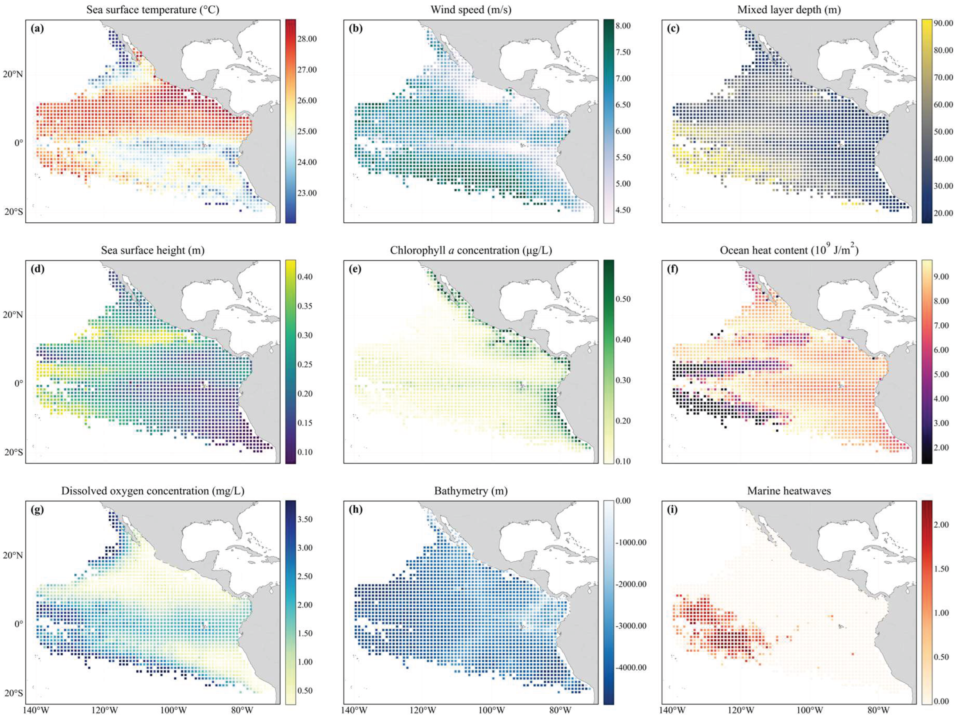
Figure 2.
Conceptual framework of the physics-guided advection-diffusion-reaction (PhyG-ADR) model for simulating the spatiotemporal dynamics of bigeye tuna.
Figure 2.
Conceptual framework of the physics-guided advection-diffusion-reaction (PhyG-ADR) model for simulating the spatiotemporal dynamics of bigeye tuna.
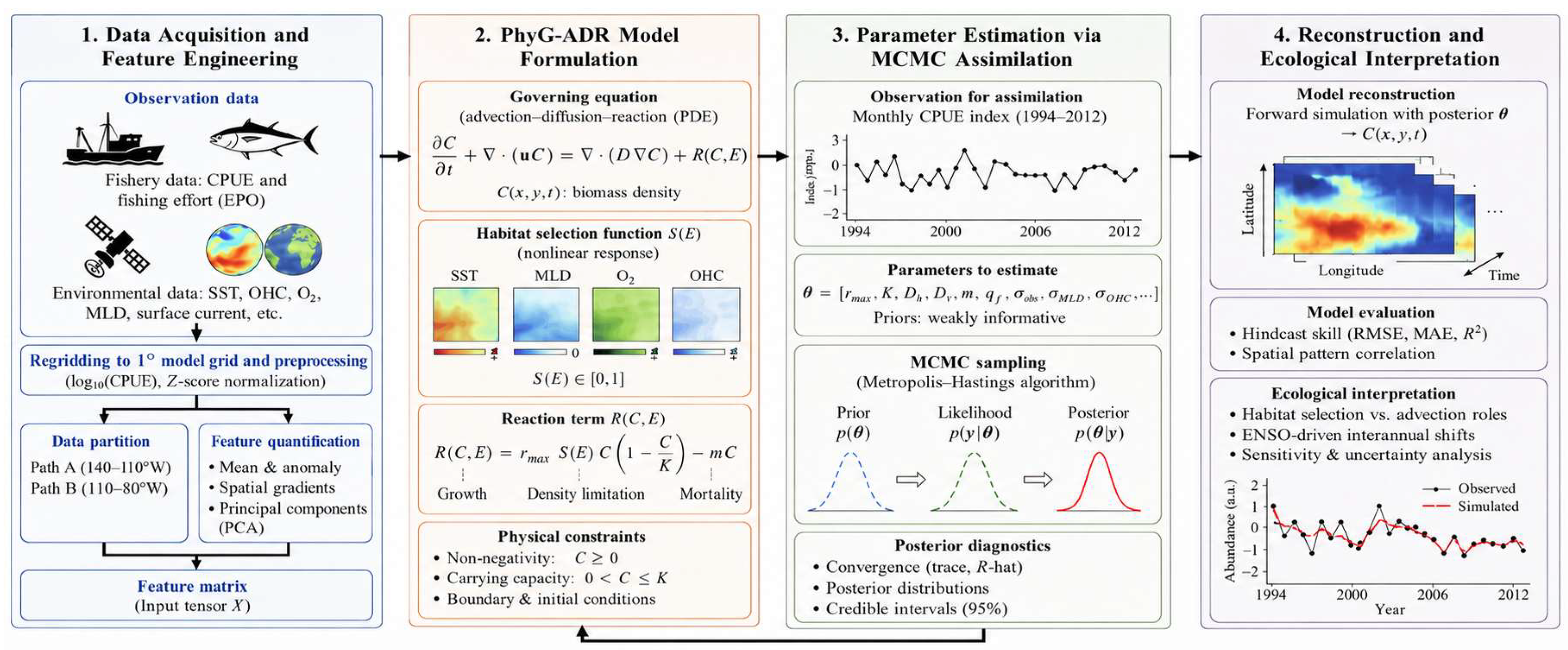
Figure 3.
MCMC convergence diagnostics and posterior distributions for three key model parameters[4]: , , and . Left column (a, c, e): Trace plots showing parameter samples over iterations, with the gray shaded region representing the burn-in period (40,000–60,000 iterations) and the blue region representing the retained samples (60,000–75,000 iterations). Red lines indicate the running mean, confirming chain stationarity. Right column (b, d, f): Corresponding kernel density estimates of the posterior distributions, based on N=36800 retained samples.
Figure 3.
MCMC convergence diagnostics and posterior distributions for three key model parameters[4]: , , and . Left column (a, c, e): Trace plots showing parameter samples over iterations, with the gray shaded region representing the burn-in period (40,000–60,000 iterations) and the blue region representing the retained samples (60,000–75,000 iterations). Red lines indicate the running mean, confirming chain stationarity. Right column (b, d, f): Corresponding kernel density estimates of the posterior distributions, based on N=36800 retained samples.
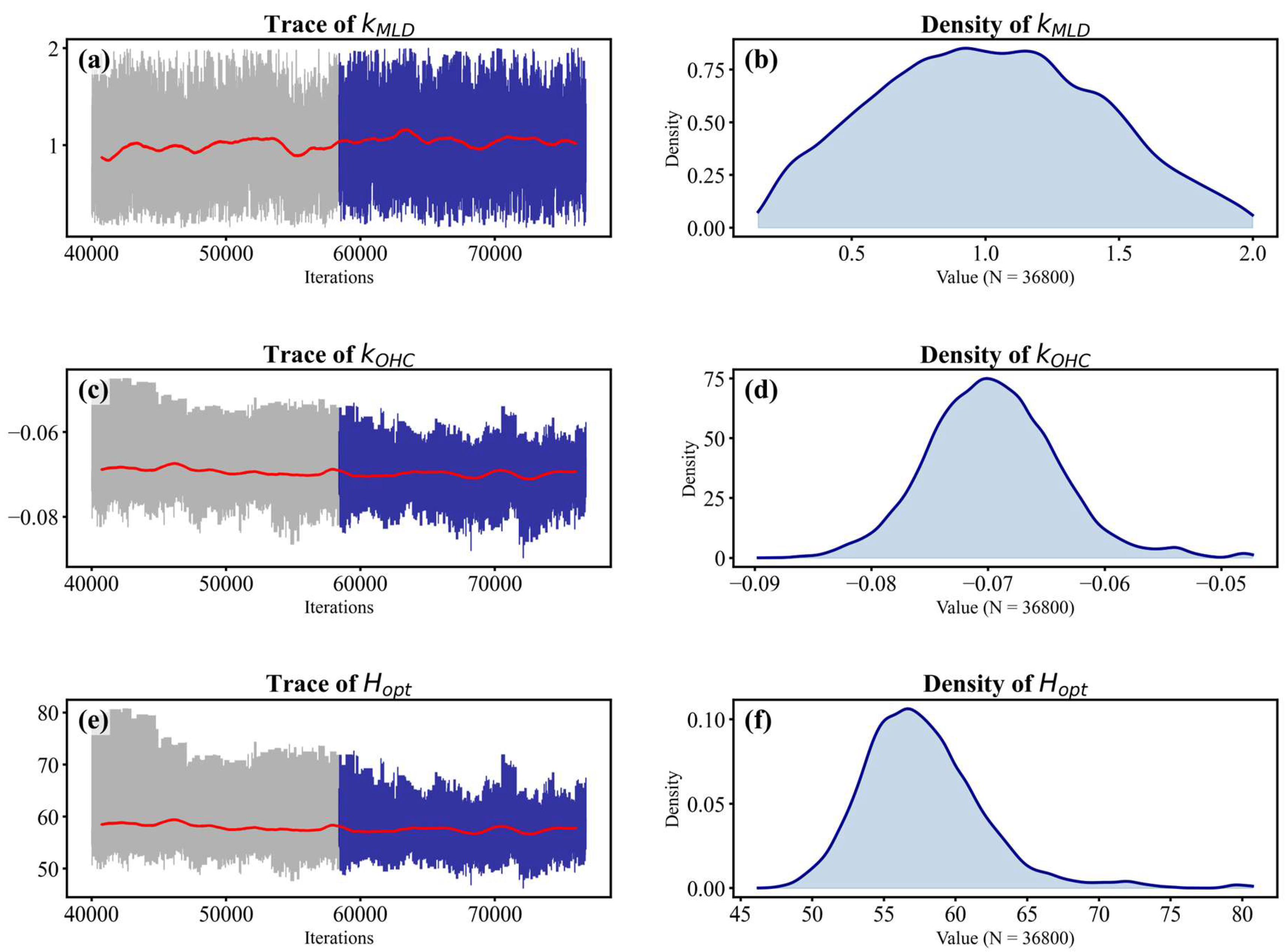
Figure 4.
Taylor diagram comparing the performance of the PhyG-ADR model and three benchmark statistical models (GAM, SVR, XGBoost) in reproducing the spatiotemporal variability of bigeye tuna abundance. The angular axis represents the correlation coefficient with observations, the radial axis represents the standard deviation of model predictions, and the red dashed contours denote the centered root-mean-square error (RMSE). The PhyG-ADR model (red dot) exhibits the highest correlation coefficient and the closest match to the observed variability amplitude, outperforming all benchmark models.
Figure 4.
Taylor diagram comparing the performance of the PhyG-ADR model and three benchmark statistical models (GAM, SVR, XGBoost) in reproducing the spatiotemporal variability of bigeye tuna abundance. The angular axis represents the correlation coefficient with observations, the radial axis represents the standard deviation of model predictions, and the red dashed contours denote the centered root-mean-square error (RMSE). The PhyG-ADR model (red dot) exhibits the highest correlation coefficient and the closest match to the observed variability amplitude, outperforming all benchmark models.
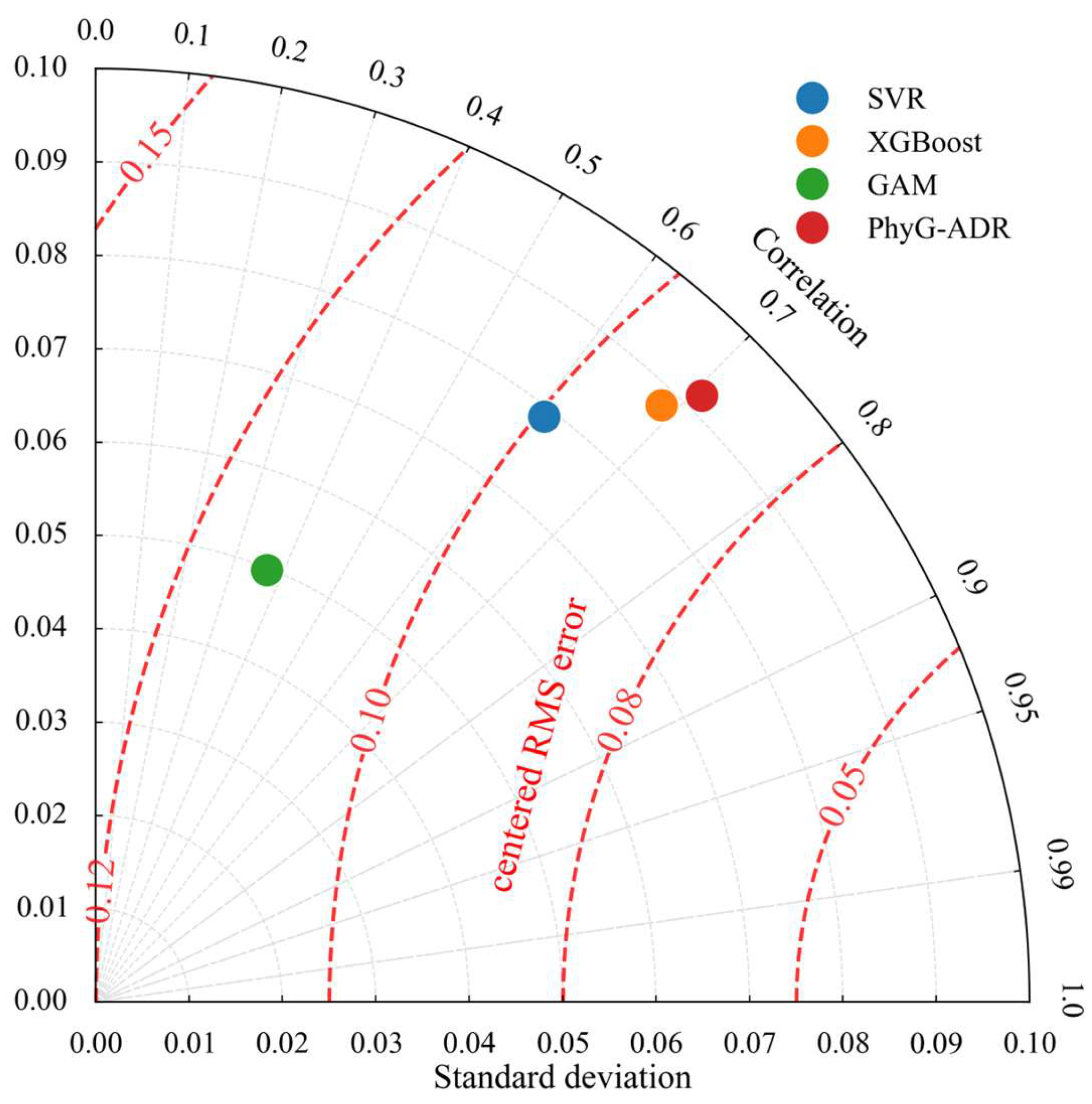
Figure 5.
Spatial distributions of observed and model-predicted mean bigeye tuna CPUE and prediction residuals in the eastern Pacific Ocean during 1994–2012.
Figure 5.
Spatial distributions of observed and model-predicted mean bigeye tuna CPUE and prediction residuals in the eastern Pacific Ocean during 1994–2012.
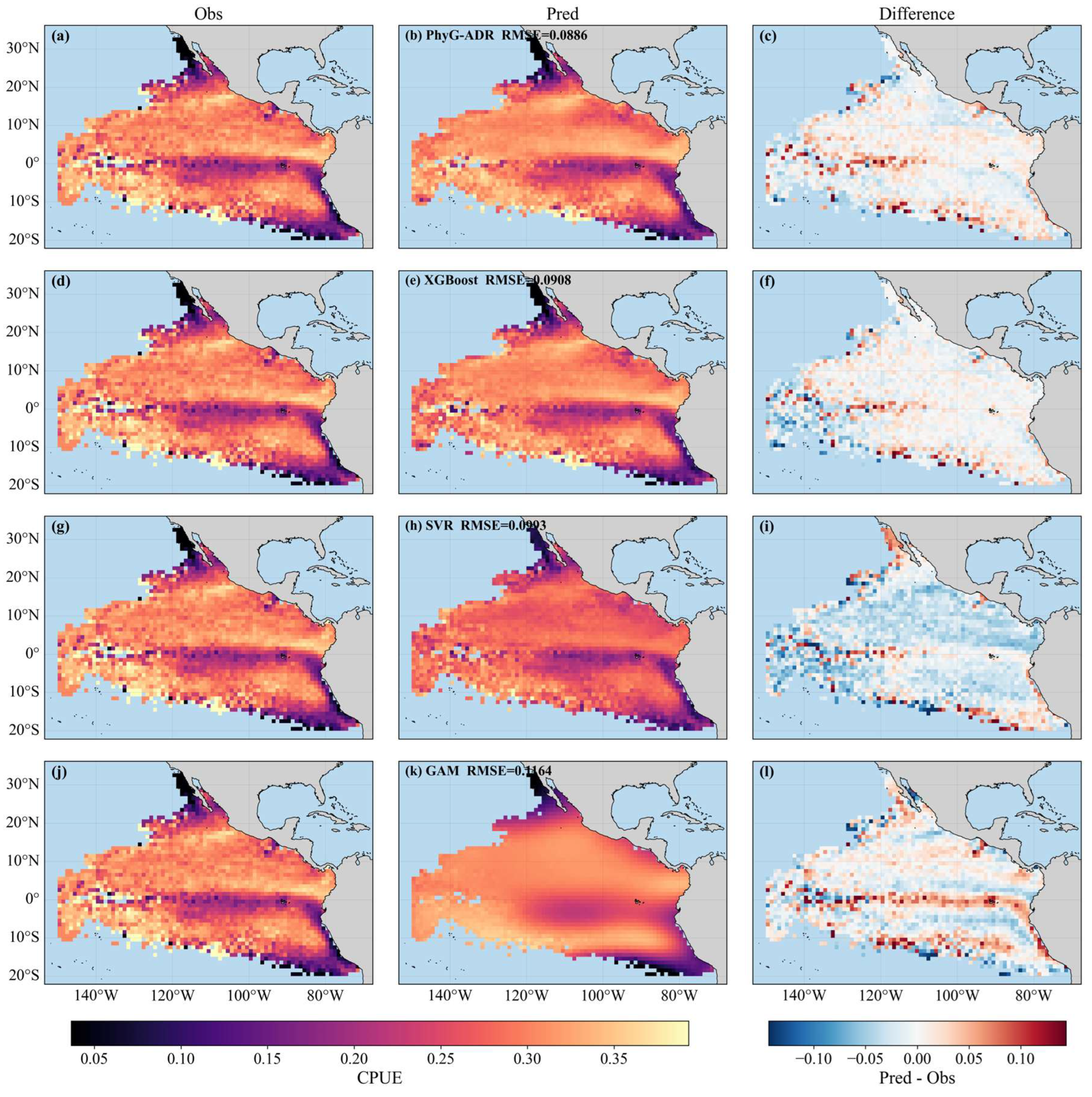
Figure 6.
Responses of bigeye tuna abundance to sea surface temperature (SST) under different carrying capacity scenarios. (a) Raw mean abundance index across SST gradients for the baseline carrying capacity and ±50% capacity scenarios. (b) Normalized abundance index (0–1 range) showing the thermal niche shape under each scenario. Despite large variations in total abundance magnitude across scenarios, the optimal temperature range and overall thermal response pattern remain consistent, demonstrating the robustness of the estimated fundamental thermal niche to changes in carrying capacity.
Figure 6.
Responses of bigeye tuna abundance to sea surface temperature (SST) under different carrying capacity scenarios. (a) Raw mean abundance index across SST gradients for the baseline carrying capacity and ±50% capacity scenarios. (b) Normalized abundance index (0–1 range) showing the thermal niche shape under each scenario. Despite large variations in total abundance magnitude across scenarios, the optimal temperature range and overall thermal response pattern remain consistent, demonstrating the robustness of the estimated fundamental thermal niche to changes in carrying capacity.
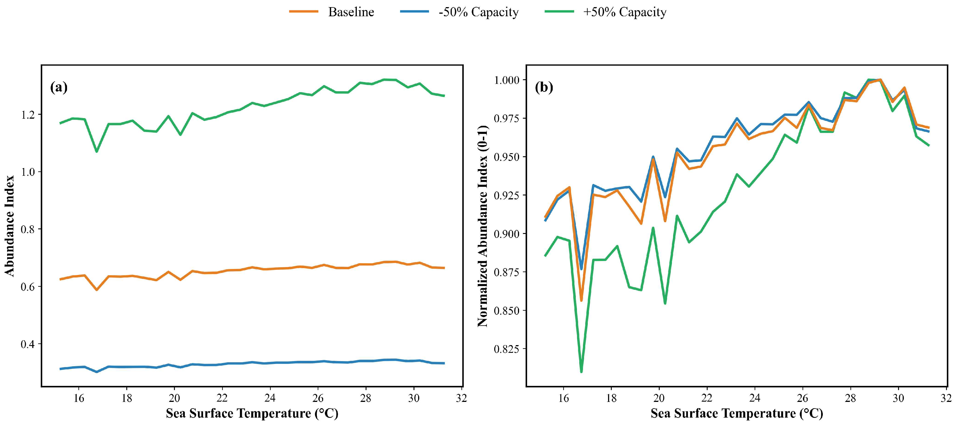
Figure 7.
Time-series comparison of the observed and PhyG-ADR-reconstructed monthly mean relative-abundance index of bigeye tuna in the eastern Pacific Ocean during 1994–2012.
Figure 7.
Time-series comparison of the observed and PhyG-ADR-reconstructed monthly mean relative-abundance index of bigeye tuna in the eastern Pacific Ocean during 1994–2012.
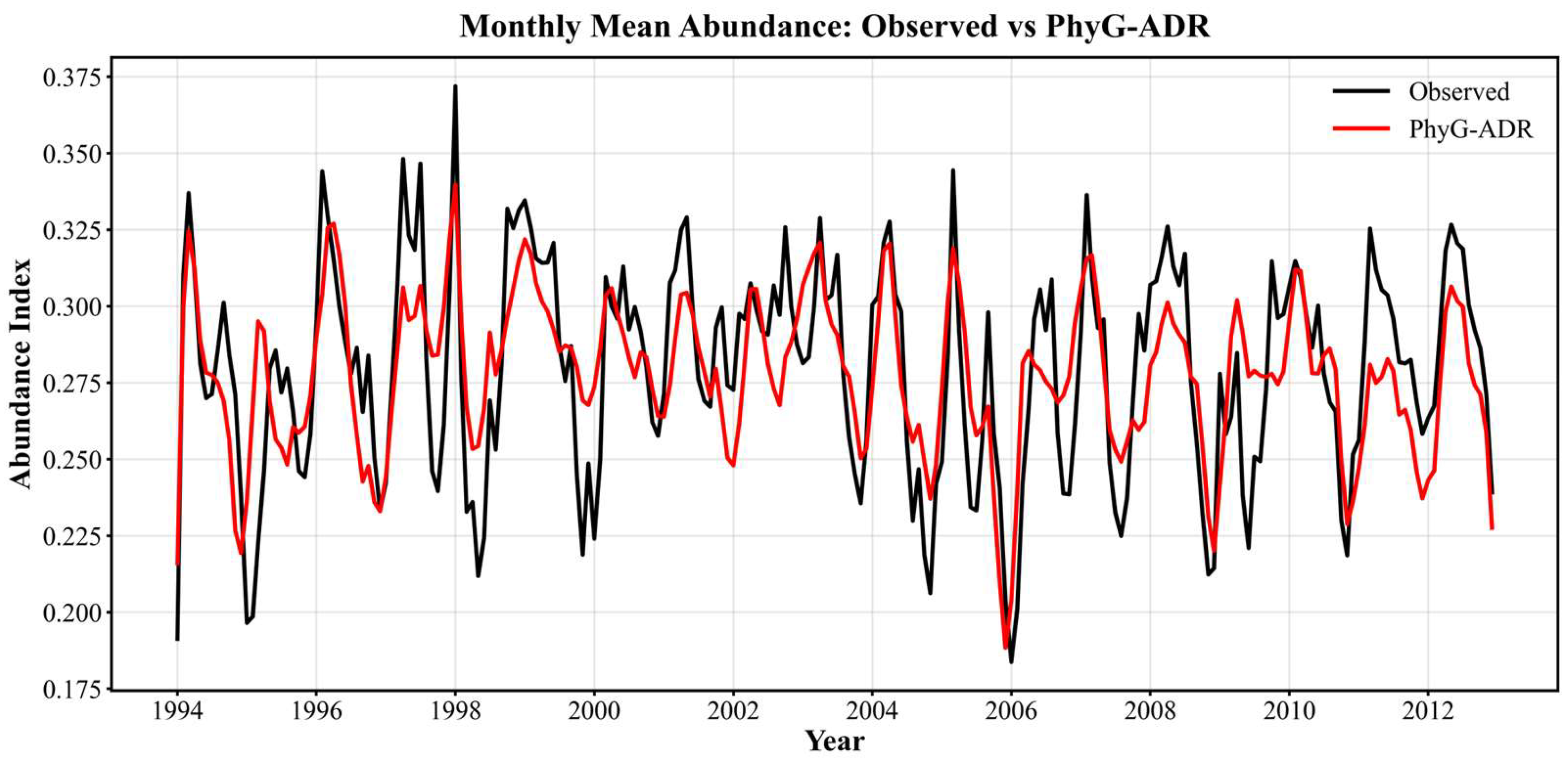

Table 1.
Performance comparison of the PhyG-ADR model and three benchmark statistical models on the test dataset, measured by the root-mean-square error (RMSE) of predicted bigeye tuna abundance.
Table 1.
Performance comparison of the PhyG-ADR model and three benchmark statistical models on the test dataset, measured by the root-mean-square error (RMSE) of predicted bigeye tuna abundance.
| Model | RMSE | Description |
|---|---|---|
| PhyG-ADR | 0.0886 | Physics-guided advection-diffusion-reaction model |
| XGBoost | 0.0908 | Gradient-boosted decision tree model |
| SVR | 0.0993 | Support vector regression with radial basis kernel |
| GAM | 0.1163 | Generalized additive model with spline smoothers |
Disclaimer/Publisher’s Note: The statements, opinions and data contained in all publications are solely those of the individual author(s) and contributor(s) and not of MDPI and/or the editor(s). MDPI and/or the editor(s) disclaim responsibility for any injury to people or property resulting from any ideas, methods, instructions or products referred to in the content. |
© 2026 by the authors. Licensee MDPI, Basel, Switzerland. This article is an open access article distributed under the terms and conditions of the Creative Commons Attribution (CC BY) license (http://creativecommons.org/licenses/by/4.0/).
Copyright: This open access article is published under a Creative Commons CC BY 4.0 license, which permit the free download, distribution, and reuse, provided that the author and preprint are cited in any reuse.