

Submitted:
06 August 2026
Posted:
06 August 2026
You are already at the latest version
Abstract
Glacier collapse hazard events have become increasingly frequent on the Tibetan Plateau under climate warming. However, the spatiotemporal evolution of multi-source remote sensing-based precursory signals before glacier collapse remains poorly understood. In this study, multi-source remote sensing datasets acquired during 1990–2016 were used to systematically investigate the pre-collapse evolution of Aru 53 and Aru 50 Glacier in terms of glacier geometry, surface elevation, glacier surface velocity (GSV), surface albedo, glacier surface temperature (GST), and surface synthetic aperture radar (SAR) backscatter coefficient. The results show that both glaciers experienced continuous terminus retreat, accompanied by upstream surface lowering and downstream surface thickening within the collapse zone. GSV increased markedly. Prior to collapse, extensive crevasses developed in the central and frontal parts of Aru 53, accompanied by a progressive increase in SAR backscatter coefficient. The enhanced SAR signals spatially coincided with regions experiencing pronounced surface structural changes. In contrast, decreases in surface albedo and increases in GST did not exhibit distinctive pre-collapse signatures for either glacier. Overall, the characteristic pattern of upstream thinning coupled with downstream thickening, anomalous acceleration of GSV, and rapid crevasse development are identified as the key remote sensing precursors of glacier instability.
Keywords:
multi-source remote sensing
; Aru Glaciers
; instability evolution
; precursory characteristics
1. Introduction
Under the ongoing global warming, the Tibetan Plateau, one of the most climate-sensitive regions on Earth, has experienced a warming rate significantly higher than the global average [1,2,3,4]. This accelerated warming has led to a continuous decline in glacier stability across the region [5,6] In recent years, cryospheric hazards, such as glacier collapses, glacial lake outburst floods (GLOFs), and glacier-related debris flows, have occurred with increasing frequency [7,8,9], posing substantial threats to downstream infrastructure, ecosystems, and local communities [10,11].
Glaciers are complex systems governed by the combined effects of climatic forcing and internal thermomechanical processes. Their evolution is influenced by multiple factors, including air temperature, precipitation, topographic conditions, glacier geometry, geothermal activity, and seismic disturbances [12,13]. Previous studies have shown that glaciers approaching an unstable state often exhibit characteristic precursory signals, such as accelerated surface motion, anomalous elevation changes, and extensive crevasse development [14,15,16]. Multi-source remote sensing has become an indispensable tool for long-term glacier monitoring and has emerged as a key approach for detecting glacier instability. Besides conventional indicators such as glacier area, length, elevation, and glacier surface velocity (GSV), new parameters including glacier surface albedo, glacier surface temperature (GST), and synthetic aperture radar (SAR) backscatter coefficient can provide useful information on glacier evolution from different perspectives, offering a more comprehensive framework for investigating glacier instability.
On July 17 and September 21, 2016, two catastrophic glacier collapses occurred at Aru 53 and Aru 50 Glacier on the western Tibetan Plateau [14]. The collapse volumes were estimated to be approximately 70 × 10⁶ m³ and 100 × 10⁶ m³ respectively [14], These events have caused severe damage to downstream pastures and infrastructure, resulting in casualties and substantial livestock losses [17]. Since then, extensive studies have investigated these events using remote sensing observations, numerical simulations, and coupled thermo-hydro-mechanical analyses. Using the Corona, Landsat, TanDEM-X, ASTER DEM, and ICESat datasets, Kääb et al. [14] reconstructed the long-term evolution of glaciers and identified surge-like acceleration and rapid crevasse development prior to collapse, suggesting that enhanced basal meltwater may have acted as a critical triggering factor. Gilbert et al. [18] combined remote sensing observations with thermo-mechanical modeling to reconstruct glacier velocity fields and stress distributions, concluding that glacier thickening, mass transport, and evolving thermal and hydrological conditions collectively contribute to progressive destabilization. Based on multi-source DEMs and historical imagery, Zhang et al. [19,20] demonstrated that both glaciers transitioned from slight thinning to substantial thickening after 2000, accompanied by positive mass balances that increased the instability risk. Recently, Jiang et al. [21] developed a coupled thermo-hydro-mechanical model integrated with a finite element–smoothed particle hydrodynamics (FE–SPH) framework to reproduce the entire process from instability development to collapse and runout, providing further insights into the underlying mechanisms.
Although previous studies have investigated glacier instability from the perspectives of climatic forcing, mass balance, and thermo-hydro-mechanical processes, most have focused on static comparisons before and after collapse events or have relied primarily on average indicators, such as GSV and elevation change. Consequently, the spatiotemporal co-evolution of multiple remote-sensing-derived indicators within key unstable regions remains insufficiently characterized. In particular, potentially important precursory signals, including changes in albedo, GST, SAR backscatter, and crevasse development during the instability incubation stage, have not been comprehensively integrated and evaluated. Therefore, there is an urgent need for a long-term, multi-source remote sensing framework capable of systematically characterizing the evolution of glacier instability and identifying robust early warning indicators. Such an approach would help address the current limitations in recognizing critical precursory anomalies and contribute to establishing more unified criteria for glacier instability assessment.
In this study, Aru 53 and Aru 50 Glacier were selected as the study objects. Multi-source remote sensing datasets, including Landsat, ASTER, ITS_LIVE, Sentinel-1 SAR, and meteorological reanalysis data, were integrated to systematically reconstruct the pre-collapse evolution of the two glaciers. Spatiotemporal variations, long-term trends, and pre-failure anomalies were comprehensively investigated using glacier geometry (1991–2015), surface elevation (2003–2015), GSV (1990–2016), surface albedo (2000–2015), GST (1997–2015), and SAR backscatter coefficient (2014.12–2016.4). Based on these multi-source remote sensing indicators, potential precursory signals associated with glacier instability were identified to improve the early detection, hazard assessment, and monitoring of catastrophic glacier collapses in high mountain regions.
2. Study Area and Datasets
2.1. Study Area
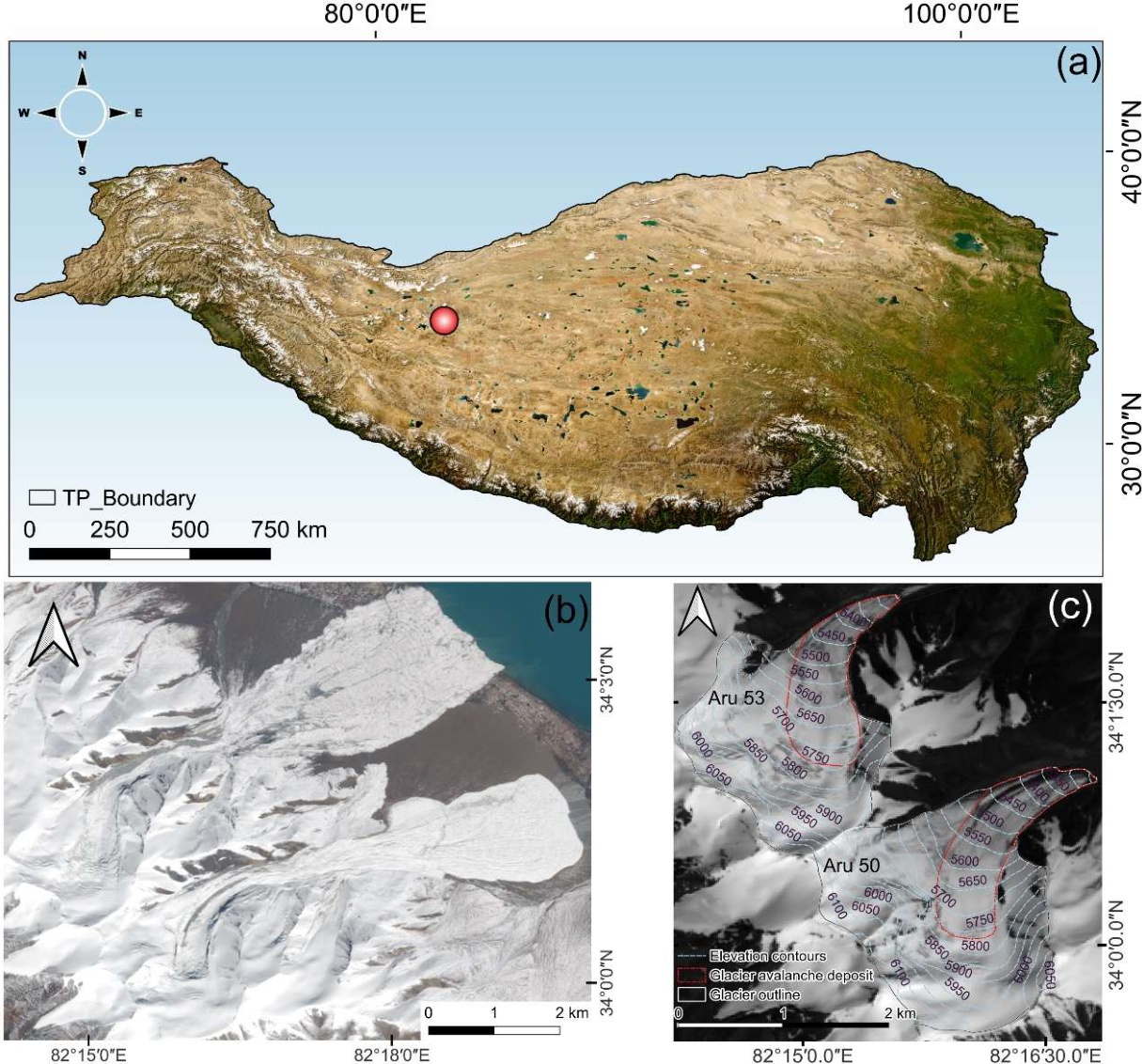
The study area is located in the western Tibetan Plateau (33.9°–34.2°N, 82.0°–82.3°E), adjacent to Aru Co, at elevations ranging from approximately 4,900 to 6,400 m a.s.l. Glaciers in this region are primarily distributed above 5,000 m. These glaciers are typical continental glaciers, characterized by predominantly cold-based conditions and a frozen ice–bed interface [20]. The regional climate is mainly controlled by the westerlies and is characterized by cold and arid conditions, with a mean annual air temperature of approximately −10 °C. Precipitation is concentrated mainly during the summer months, from June to September [17,22]. This study focuses on Aru 53 and Aru 50, both of which are low-gradient valley glaciers with similar sizes and topographic settings.
Figure 1.
Location and imagery of the Aru Glacier collapse in Tibet. (a) Location of the Aru glaciers in Tibet (TP denotes the Tibetan Plateau). (b) Sentinel-2 image after the collapse on October 16, 2016. (c) Light blue dashed lines represent elevation contours (vertical datum: WGS84) of Aru 53 and 50, overlaid on the background Sentinel-2 image from April 21, 2016. The red lines indicate the collapsed glacier areas, and the white lines indicate the glacier outlines.
Figure 1.
Location and imagery of the Aru Glacier collapse in Tibet. (a) Location of the Aru glaciers in Tibet (TP denotes the Tibetan Plateau). (b) Sentinel-2 image after the collapse on October 16, 2016. (c) Light blue dashed lines represent elevation contours (vertical datum: WGS84) of Aru 53 and 50, overlaid on the background Sentinel-2 image from April 21, 2016. The red lines indicate the collapsed glacier areas, and the white lines indicate the glacier outlines.
2.2. Datasets
This study integrated multiple remote sensing datasets and meteorological reanalysis products to characterize the long-term evolution of the Aru glaciers (Table 1). ASTER-derived digital elevation models (DEMs) and glacier outlines from the Randolph Glacier Inventory Consortium (RGI 7.0; RGI Consortium, 2023) were used to quantify glacier surface elevation changes and refine the glacier boundaries. Landsat multispectral imagery (TM, ETM+, and OLI) was used for glacier boundary delineation, crevasse mapping, GSV retrieval, and GST estimation (Section 3.3). Long-term glacier surface velocity data (1990–2015) were obtained from the Inter-Mission Time Series of Land Ice Velocity and Elevation (ITS_LIVE) Regional Velocity Mosaics dataset [23]. In addition, Sentinel-1 GRD SAR imagery was used to derive glacier surface backscatter characteristics, and the MODIS MCD43A3 Version 6.1 albedo product was utilized to investigate temporal variations in surface albedo. Meteorological variables, including air temperature and precipitation, were obtained from the ERA5 reanalysis dataset and complemented with daily precipitation estimates from the NASA Integrated Multi-satellite Retrievals for GPM (IMERG) product [24].
3. Methods and Uncertainty Assessment
3.1. Glacier Boundary Extraction
In this study, glacier extents from 1990 to 2016 were delineated using Landsat satellite imagery based on the Normalized Difference Snow Index (NDSI). The NDSI was calculated as follows:
where Green and SWIR represent the surface reflectance in the green and shortwave infrared spectral regions, respectively. Following the approach proposed by Paul et al. [25], the automatically extracted glacier outlines were further refined according to local conditions and subsequently corrected by comparing them with the RGI 7.0 inventory and manual visual interpretation.
The accuracy of glacier boundary delineation is primarily constrained by the spatial resolution of remote sensing data and co-registration error in multisource datasets. Following the uncertainty assessment methods proposed by Bolch et al. [26] and Paul et al. [27], the uncertainties of glacier area (EA) and glacier length (EL) for an individual glacier were estimated as follows:
where n represents the total number of pixels along the glacier boundary, while is considered negligible and therefore omitted from the calculation.
3.2. Surface Elevation and Registration
To obtain information on glacier surface elevation changes, the MMASTER method [28] was used to generate DEM data for 2003, 2007, 2011, 2013, 2014, and 2015 using ASTER stereo pairs. Subsequently, the demcoreg tool developed by Shean et al. [29] was used to register multiphasehase DEMs. This tool is based on the DEM registration method proposed by Nuth and Kääb [30](Equation 3), which utilizes the relationship between elevation differences in ice-free flat areas and terrain parameters to iteratively correct horizontal and vertical deviation errors between DEMs, thereby eliminating deviations caused by horizontal displacement between different DEMs and improving the accuracy and reliability of the calculation results (Figure 2).
where is the elevation difference between the reference DEM and the DEM to be co-registered; and represent the terrain slope and aspect, respectively. a is the amplitude of the cosine function, which characterizes the magnitude of the aspect-dependent elevation error, b is the phase parameter describing the direction of the horizontal displacement, and c is a constant term accounting for the overall vertical offset of the DEM.
An accurate assessment of elevation uncertainty requires the identification of stable, non-glacierized reference areas with terrain characteristics (e.g., slope and aspect) comparable to those of glacier surfaces. Therefore, the Normalized Median Absolute Deviation (NMAD) was employed as a robust statistical measure of elevation error, as it is less sensitive to outliers than conventional standard deviation metrics [30,31]:
where denotes the elevation difference series over the stable terrain. The overall uncertaintywas estimated by accounting for the systematic residual error introduced during DEM co-registration . Following Hugonnet et al. [32], was set to 3 m.
Considering that spatial autocorrelation reduces the number of truly independent observations, the effective number of independent samples was used to adjust the uncertainty of the mean elevation change, following the method of Gardelle et al. [33].
where PS is the pixel size, and d is the spatial decorrelation distance (0.5 km in this study).
3.3. Glacier Surface Velocity
A long-term GSV record was derived from the ITS_LIVE dataset, from which annual mean GSV of the Aru glaciers were obtained for the period 1990–2015. However, owing to its spatial resolution of 120 m, the dataset is insufficient to capture the detailed spatial variations in glacier motion for Aru 53 and Aru 50. Therefore, this study employed multi-temporal Landsat optical imagery and the PyCorr_Iceflow algorithm [34] to derive higher-resolution GSV fields. Image pairs covering the period from 1 December 2013 to 24 June 2016 were selected, including 20131201–20141126, 20141126–20151028, 20151028–20160201, 20160201–20160304, 20160304–20160421, and 20160421–20160624. The mean pre-collapse GSV for 2016 was calculated from the velocity estimates obtained during the period 20151028–20160624. PyCorr_Iceflow is based on normalized cross-correlation (NCC) feature matching and derives glacier surface velocities by tracking the displacement of surface texture patterns between optical image pairs. Compared with the long-term averaged ITS_LIVE product, this approach is better suited for resolving short-term velocity variations and the detailed spatial patterns of glacier motion.
Uncertainty assessment was conducted using residual analysis over stable, ice-free terrain with slopes lower than 15°, where the dispersion of residuals provides an estimate of random errors [35]. The estimated velocity uncertainties over stable areas were 0.004 m d⁻¹ for the ITS_LIVE dataset and 0.02 m d⁻¹ for Landsat-derived velocities. Both uncertainty values were substantially smaller than the observed glacier surface velocities, indicating that the derived velocity measurements were reliable [36].
3.4. Glacier Surface Albedo, Temperature, and Backscattering Coefficient
Surface albedo (2000-2015) and GST data(1997-2015) for Aru 53 and Aru 50 were obtained from the Google Earth Engine (GEE) platform, together with Sentinel-1 backscatter coefficient (σ⁰) data covering December 2014 to June 2016.
Albedo data were derived from the MODIS MCD43A3 Version 6.1 product, which provides shortwave white-sky albedo estimates based on multi-angular observations and inversion of the Bidirectional Reflectance Distribution Function (BRDF) model, with a spatial resolution of 500 m. This product was used to generate glacier albedo records for 2000–2015. For the pre-MODIS period, the glacier surface albedo was retrieved from Landsat imagery using the narrowband-to-broadband conversion algorithm proposed by Liang [37]. Following the validation results reported by Yue et al. [38] for Urumqi - 1 in the Tianshan Mountains and the assessment of Wang et al. [39], the uncertainty of the albedo estimates derived from both MODIS and Landsat data was assumed to be ±0.05.
The GST was obtained from the Landsat Collection 2 Level-2 Surface Temperature products, including data from the Landsat 5 TM, Landsat 7 ETM+, and Landsat 8 OLI/TIRS sensors. To ensure data quality, cloud-contaminated and cloud-shadow pixels were removed using the QA_PIXEL quality-assessment band. The digital number (DN) values were then converted to the actual glacier surface temperature according to the scale factors provided in the official product documentation [40,41]:
where DN is the digital number of the thermal infrared temperature band, and GST is the glacier surface temperature expressed in °C. To minimize the influence of variations in observation frequency on long-term trend analysis, seasonal mean GST values were first calculated for spring, summer, autumn, and winter, and subsequently averaged to derive the annual mean GST. Years with missing data in any season were excluded from the analysis. Following the validation results reported for the Third Pole region by Ren et al., the uncertainty of the GST in this study was estimated to be ± 1.46 °C.
The backscatter coefficient data were derived from Sentinel-1 Ground Range Detected (GRD) products, covering the period from December 2014 to June 2016. The backscatter coefficient (σ⁰) was calculated using the method proposed by Ulaby and Long [42]:
3.5. Standardization of Characteristic Indicators
For ease of comparison among the pre-collapse variations in glacier surface elevation change, GSV, albedo, GST, and SAR backscatter coefficient, all time-series indicators were standardized using the Z-score normalization method to eliminate the influence of different units and value ranges. The standardized value was calculated as follows [43]:
where Zi is the standardized (Z-score) value, Xi is the observed value at time i, μ is the mean of the entire time series, and σ is the standard deviation of the entire time series.
4. Result
4.1. Temporal Evolution of Glacier Geometry
Between 1991 and 2015, both the Aru 53 and Aru 50 glaciers exhibited an overall retreating trend (Figure 3). The length of the Aru 53 Glacier decreased from 3.56 ± 0.02 km to 3.23 ± 0.02 km, corresponding to a cumulative retreat of 0.33 ± 0.02 km (9.27%) and an average retreat rate of 0.13 ± 0.02 km·a-1. In comparison, the Aru 50 Glacier experienced a more pronounced retreat, with its length decreasing from 3.57 ± 0.02 km to 3.20 ± 0.02 km, resulting in a total retreat of 0.37 ± 0.02 km (10.36%) and an average retreat rate of 0.15 ± 0.02 km·a-1. Although both glaciers continuously retreated from 1991 to 2014, contrasting behaviors emerged during 2014–2015. The length of the Aru 53 Glacier increased by 1.25% (from 3.19 ± 0.02 to 3.23 ± 0.02 km), representing the first positive advance observed during the study period, whereas the Aru 50 Glacier continued to retreat, with a further reduction of 0.31%.
Regarding area changes (Figure 3), the Aru 53 and Aru 50 glaciers lost 0.11 km² (2.90%) and 0.19 km² (3.97%) of their total areas, respectively, between 1991 and 2015. The rates of area reduction gradually slowed from 2000 to 2014. Notably, the area of the Aru 53 Glacier increased by 0.03 km² (0.75%) during 2014–2015, indicating glacier advance or surge-like behavior, whereas the Aru 50 Glacier continued to experience area loss throughout the same period.
4.2. Surface Elevation Change
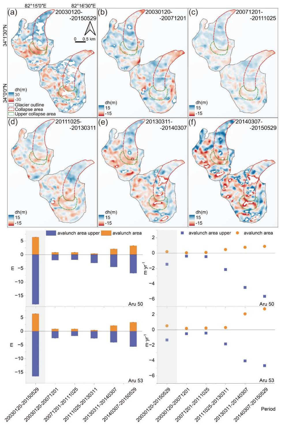
The multi-temporal DEM differencing results were derived from ASTER stereo image pairs (Figure 4, Figure S1) revealed an overall surface elevation increase for both the Aru 53 and Aru 50 glaciers during 2003–2015. The Aru 53 Glacier exhibited a cumulative thickening of 3.50 ± 0.05 m, corresponding to an average rate of 0.29 ± 0.01 m yr⁻¹, which was greater than that of the Aru 50 Glacier, where the cumulative thickening reached 2.15 ± 0.05 m (0.17 ± 0.01 m yr⁻¹).
The collapse-prone zones (red areas in Figure 4) experienced persistent thickening during the entire observation period. Cumulative thickening reached 6.39 ± 0.05 m (0.52 ± 0.01 m yr⁻¹) for Aru 53 Glacier and 2.19 ± 0.05 m (0.18 ± 0.01 m yr⁻¹) for Aru 50 Glacier, respectively. Notably, thickening accelerated markedly after 2013, with maximum annual thickening rates of 2.72 m yr⁻¹ and 0.84 m yr⁻¹ for the Aru 53 and Aru 50 glaciers, respectively.
In contrast, the upper glacier regions (green areas in Figure 4) showed persistent surface lowering throughout the year. Between 2003 and 2015, cumulative thinning reached 16.47 ± 0.05 m for the Aru 53 Glacier and 18.11 ± 0.05 m for the Aru 50 Glacier, corresponding to mean thinning rates of 1.33 ± 0.01 m yr⁻¹ and 1.46 ± 0.01 m yr⁻¹, respectively. Throughout the observation period, the upper regions of both glaciers remained in a state of continuous thinning, with thinning rates increasing significantly over time. For the Aru 53 Glacier, the thinning rate increased from 0.51 ± 0.01 m yr⁻¹ in 2003 to 4.68 ± 0.03 m yr⁻¹ in 2015, representing an approximately eightfold increase. For the Aru 50 Glacier, the thinning rate increased from 0.41 ± 0.01 m yr⁻¹ to 5.56 ± 0.03 m yr⁻¹ over the same period, corresponding to an increase of more than thirteenfold.
Figure 3.
Multi-temporal evolution of glacier outlines for the Aru 53 and Aru 50 glaciers (1990–2015). (a) and (b) show zoomed-in views of Aru 53 and Aru 50, respectively. Temporal evolution of glacier length (d) and area (e) for the Aru 53 and Aru 50 glaciers (1991–2015).
Figure 3.
Multi-temporal evolution of glacier outlines for the Aru 53 and Aru 50 glaciers (1990–2015). (a) and (b) show zoomed-in views of Aru 53 and Aru 50, respectively. Temporal evolution of glacier length (d) and area (e) for the Aru 53 and Aru 50 glaciers (1991–2015).
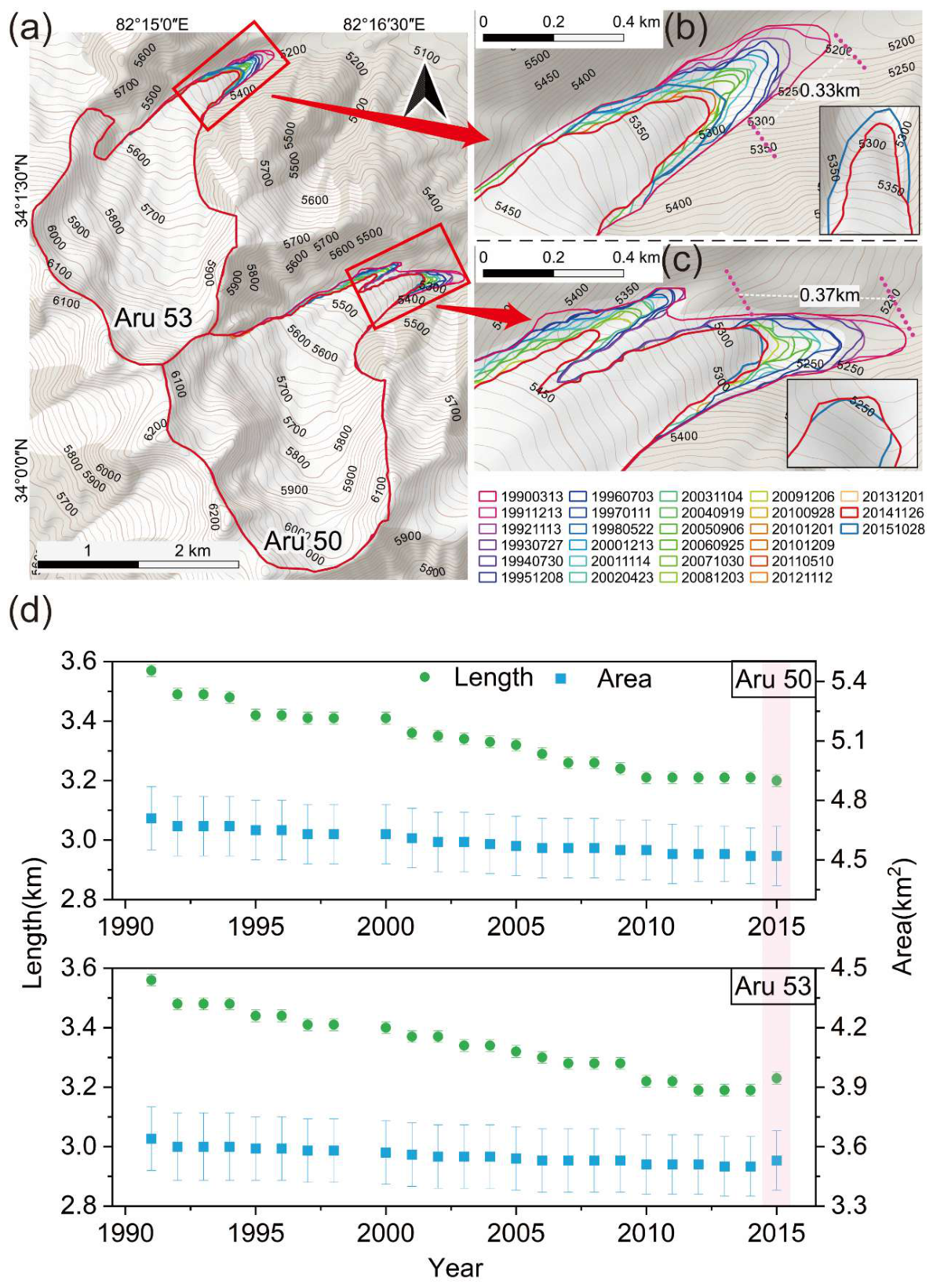
Figure 4.
Multitemporal surface elevation changes of the Aru 53 and Aru 50 glaciers (2003–2015). Subpanels illustrate elevation differences for sequential intervals: (a) cumulative change from January 20, 2003, to May 29, 2015; (b) January 20, 2003, to December 1, 2007; (c) December 1, 2007, to October 25, 2011; (d) October 25, 2011, to March 11, 2013; (e) March 11, 2013, to March 7, 2014; and (f) March 7, 2014, to May 29, 2015. Values represent elevation loss (negative) or gain (positive) in meters, derived from DEM differencing of ASTER stereo imagery. (g) Mean surface elevation change in the collapse area (red region in panel a) during 2003–2015. (h) Mean surface elevation change in the upper part of the collapse area (green region in panel (a) during 2003–2015.
Figure 4.
Multitemporal surface elevation changes of the Aru 53 and Aru 50 glaciers (2003–2015). Subpanels illustrate elevation differences for sequential intervals: (a) cumulative change from January 20, 2003, to May 29, 2015; (b) January 20, 2003, to December 1, 2007; (c) December 1, 2007, to October 25, 2011; (d) October 25, 2011, to March 11, 2013; (e) March 11, 2013, to March 7, 2014; and (f) March 7, 2014, to May 29, 2015. Values represent elevation loss (negative) or gain (positive) in meters, derived from DEM differencing of ASTER stereo imagery. (g) Mean surface elevation change in the collapse area (red region in panel a) during 2003–2015. (h) Mean surface elevation change in the upper part of the collapse area (green region in panel (a) during 2003–2015.
4.3. GSV Change
Based on the ITS_LIVE GSV product (Figure 5a), both Aru 53 and Aru 50 remained in a relatively slow and stable flow regime from 1990 to 2015. The mean surface velocity of Aru 53 ranged from 0.01 ± 0.004 m·d-1 to 0.02 ± 0.004 m·d-1, whereas that of Aru 50 varied between 0.01 ± 0.004 m·d-1 and 0.03 ± 0.004 m·d-1.
The PyCorr_Iceflow-derived annual mean GSV for 2014 (1 December 2013–26 November 2014; Figure 5b) was 0.03 ± 0.02 m·d-1 for both Aru 53 and Aru 50 glaciers, which agrees well with the 2014 ITS_LIVE estimates (0.02 ± 0.004 m·d-1). The agreement between the two independent velocity products, within their uncertainty ranges, demonstrates the robustness of the derived velocity measurements.
Both glaciers exhibited pronounced acceleration beginning in 2014 and entered a phase of rapid dynamic adjustment before collapse in 2016. During February–June 2016, the mean surface velocities of Aru 53 and Aru 50 reached 0.45 ± 0.02 m·d-1 and 0.42 ± 0.02 m·d-1, respectively, approximately 20 times higher than their long-term background velocities (The mean surface velocity derived from ITS_LIVE during 1990–2013 was 0.02 ± 0.004 m·d-1for both glaciers). The temporal evolution revealed a progressive acceleration before collapse. From 1 February to 4 March 2016, the mean velocities increased to 0.64 m·d-1 for Aru 53 and 0.45 m·d-1 for Aru 50, followed by a further increase during 4 March–21 April, reaching peak values of 0.82 and 0.64 m·d-1, respectively. Although velocities slightly decreased during 21 April–24 June, they remained substantially elevated (0.72 m·d-1 for Aru 53, 0.47 m·d-1 for Aru 50). Spatially, the highest velocities were concentrated within the eventual collapse zones, where distinct high-velocity bands developed prior to glacier collapse.
4.4. Surface Albedo, GST, and Radar Backscatter Coefficient (σ⁰) Variations
From 2000 to 2016, the annual mean albedo of the Aru 53 and Aru 50 glaciers exhibited pronounced interannual fluctuations, generally ranging from 0.46 to 0.58 (Figure 6a). Overall, the albedo of Aru 53 was slightly higher than that of Aru 50. Both glaciers experienced a long-term declining trend from 2000 to 2016, with the annual mean albedo decreasing from 0.58±0.05 to 0.51±0.05 for Aru 53, and from 0.50±0.05 to 0.48±0.05 for Aru 50.
On a seasonal scale, both glaciers exhibited significant variations (Figure 6b). Albedo values during spring and autumn generally exceeded 0.55, peaking at 0.63±0.05 for Aru 53 in 2001 and 0.61±0.05 for Aru 50 in 2012. In contrast, summer albedo dropped markedly due to snowmelt and bare ice exposure, ranging from 0.46±0.05 to 0.55±0.05 for Aru 53 and from 0.47±0.05 to 0.56±0.05 for Aru 50.
Spatial slope analysis (Figure S3) revealed distinct negative albedo trends at the termini of both glaciers, indicating continuous long-term degradation; a localized area on the left side of the Aru 50 ice tongue showed particularly sharp declines in albedo. In comparison, the 28 surrounding reference glaciers exhibited smaller albedo fluctuations and more homogeneous spatial distributions. Regional comparisons indicated that the albedo variations of the Aru 53 and Aru 50 glaciers did not show anomalies that significantly distinguished them from the neighboring glaciers.
According to the GST results retrieved from Landsat data (Figure 7), the limited availability and relatively low quality of satellite imagery before 2000 resulted in greater dispersion of early GST observations, obscuring any clear long-term trends. After 2000, however, both glaciers exhibited more distinct seasonal variations in the GST. At the annual scale, the GST of both the Aru 53 and Aru 50 glaciers showed an overall increasing trend from 1990 to 2016. Seasonal analyses (Figure 7c) revealed that GST was lowest in winter, generally ranging from −21 °C to −27 °C and exhibiting considerable interannual variability, whereas summer GST was highest, mostly between −3 °C and 0 °C. The spring and autumn GST values were intermediate between these extremes. All four seasons displayed a gradual warming trend, which is consistent with the regional climate warming observed across the Tibetan Plateau.
The spatial distribution of the annual GST change rates (Figure S3) further indicated a pronounced warming trend in the glacier termini of both Aru 53 and Aru 50 glaciers. Relatively stronger warming was observed in a localized area on the left side of the tongue of the Aru 50 Glacier. Nevertheless, a comparison with 28 surrounding reference glaciers showed that both the magnitude and spatial pattern of the GST changes were broadly similar to the regional background signal. No anomalous warming features that were distinctly different from those observed in neighboring glaciers were identified.
The temporal evolution of SAR backscatter coefficient (σ⁰) during the cold seasons (December–April) from 2014 to 2016 revealed contrasting radar responses between Aru 53 and Aru 50 glaciers (Figure 8a,b). At the glacier-wide scale, Aru 53 exhibited a continuous increase in σ⁰, rising from −5.01 dB in December 2014 to −4.31 dB in April 2016 (+0.70 dB). In contrast, Aru 50 showed relatively stable σ⁰ values, varying between −4.91 and −4.65 dB (+0.26 dB), with limited interannual fluctuations.
The divergent radar responses became more pronounced immediately before collapse. During the cold season preceding the collapse events, the mean σ⁰ of Aru 53 increased markedly to −4.41 dB in 2016, whereas Aru 50 remained nearly unchanged (~−4.81 dB). Spatial analysis further revealed that the increase was concentrated within the collapse zone of Aru 53, where σ⁰ increased by 1.15 dB (from −5.59 to −4.44 dB), while the corresponding region of Aru 50 exhibited no significant change (−4.99 to −5.05 dB). In comparison, the upper glacier zones showed relatively weak temporal variations, with σ⁰ changes of only 0.18 dB and 0.03 dB for Aru 53 and Aru 50, respectively.
The spatially concentrated enhancement of σ⁰ in the collapse zone of Aru 53 coincided with the development and expansion of surface crevasses observed from optical imagery (Figure 8c–i). Before the June 2016 collapse, extensive crevasses developed along both margins of the ice tongue and propagated toward the upper glacier, particularly around the detachment area. In contrast, crevasse development on Aru 50 remained localized near the eventual detachment zone before the September 2016 collapse. These results suggest that enhanced SAR backscatter, particularly its spatial concentration within the collapse zone, may reflect progressive surface structural deterioration associated with glacier destabilization.
5. Discussion
5.1. Evolution of Multi-Source Remote Sensing Precursors Prior to Glacier Collapse
Based on multi-source remote sensing data, this study identified a sequence of pre-collapse changes in the two glaciers (Figure 9), characterized by localized elevation anomalies, accelerated GSV, and crevasse development, which is consistent with previous studies [14,18]. Furthermore, by incorporating albedo, GST, and SAR backscatter, we revealed the temporal evolution of multi-indicator responses and their potential critical transitions prior to glacier collapse.
5.1.1. Long-Term Drivers of Glacier Instability
From a regional climatic perspective, both air temperature and precipitation showed increasing trends during 1990–2016 (Figure S5), indicating an overall warm and wet climate regime. Under these conditions, glacier albedo continuously decreased, whereas GST increased, suggesting a clear glacier response to regional warming. A reduced albedo enhances the absorption of incoming shortwave radiation, whereas a higher GST promotes ice warming and meltwater production, creating favorable thermal conditions for glacier destabilization. These findings are consistent with previous studies showing that rising air temperature is a major driver of albedo decline and glacier thermal change [44,45,46]. In addition, a decrease in albedo can amplify ice melt and energy absorption, generating a positive feedback that accelerates glacier mass loss [47,48].
However, compared with neighboring non-collapsing glaciers, Aru 50 and Aru 53 did not exhibit distinct anomalies in either the albedo or GST. This suggests that the observed albedo decline and GST increase mainly reflect the widespread glacier response to regional climate warming, rather than collapse-specific signals. Therefore, the warm–wet climate regime and the associated changes in the glacier surface energy balance are more likely to represent long-term preconditioning factors for glacier instability rather than direct short-term precursors of glacier collapse.
5.1.2. Localized Elevation Anomaly
Under continued climate warming, glacier elevation changes directly reflect internal mass transport and redistribution processes. ASTER DEM differencing revealed a persistent pattern on both Aru 50 and Aru 53 since 2003, characterized by upstream thinning and pronounced thickening within the eventual collapse zone, with this trend becoming markedly stronger around 2011 (Figure 3). Given the gentle valley geometry and downstream topographic constraints, ice delivered from the upper glacier was inefficiently evacuated and progressively accumulated in the collapse-prone areas. According to the driving stress relationship (τ = ρ·g·h·sinθ), increasing ice thickness under nearly constant slope conditions leads to a higher driving stress, thereby promoting ice deformation and stress accumulation. Similar pre-collapse mass redistributions and downstream thickening have been reported for other catastrophic glacier failures [14,18], including events in the Anyemaqen Mountains, Sedongpu Basin, and Chamoli region [49,50,51,52]. These results indicate that localized thickening within the collapse zone represents a robust precursor of glacier instability and provides the mechanical conditions for subsequent acceleration and dynamic failure of the glacier.
5.1.3. Abrupt Increase in Surface Velocity
As mass and stress continuously accumulated within the collapse zone [18], the GSV remained low and relatively stable from 1990 to 2014 (Figure 5), indicating a state dominated by steady viscous creep. Since 2014, the GSV has increased rapidly to several times its long-term background level (Figure 5). Combined with the elevation-change results, the GSV anomaly exhibited a clear lag relative to localized elevation anomalies, suggesting that prolonged mass accumulation and stress buildup were initially accommodated by geometric adjustment before rapid acceleration was triggered as the system approached the critical threshold. In addition, increased meltwater input and intense precipitation under a warmer and wetter climate (Figure S5) may have reached the glacier bed through crevasses and englacial conduits, reducing effective pressure and basal friction, thereby enhancing basal sliding [14,18].
Similar precursory accelerations have been reported for other glacier collapse events. For example, glaciers in the Animaqing Mountains showed pronounced GSV acceleration before collapse [53], while velocity anomalies were also observed prior to the collapse of the Sedongpu glacier [52,54] and the Chamoli disaster [51,55]. Our results indicate a common evolution pattern characterized by localized elevation anomalies preceding velocity acceleration, followed by rapid destabilization after exceeding a critical threshold. Therefore, abrupt GSV acceleration can be regarded as a key dynamic indicator of glacier instability and is clearly expressed in the standardized time series (Figure 9).
5.1.4. Crevasse Development and SAR Backscatter Response
From the perspective of radar scattering mechanisms, σ⁰ is primarily controlled by surface roughness, dielectric properties, and volume-scattering processes [42,56]. The development of dense crevasses increases the glacier surface roughness, whereas multiple reflections and corner-reflector effects within crevasse walls enhance the SAR backscatter [57]. In this study, areas of high σ⁰ change rates spatially coincide with densely crevassed zones (Figure 8), indicating that the observed backscatter increase is mainly associated with surface structural fragmentation. The pre-collapse enhancement of σ⁰ occurred synchronously with the rapid crevasse expansion. Concurrently, glacier acceleration increases tensile stress, promoting the propagation of damage from the glacier interior to the surface and facilitating the transition from viscous creep to brittle fracture [58].
Aru 53 exhibited a stronger σ⁰ increase prior to collapse than Aru 50, although both glaciers showed pronounced crevasse expansions. Previous observations reported that, between 2014 and 2016, the number of crevasses increased from 99 to 290 and their total length from 6.2 to 16.7 km on Aru 53, whereas on Aru 50, the number increased from 64 to 85 and the total length from 3.9 to 5.5 km [17]. Similar backscatter enhancement associated with structural degradation has been documented in several glacier collapse events, including those in the Anyemaqen region, Sedongpu Glacier, and Chamoli area [51,55,59,60]. These results suggest that σ⁰ is sensitive to damage accumulation and the progressive loss of glacier surface structural integrity, highlighting its potential as a complementary remote-sensing indicator for monitoring glacier instability.
5.1.5. Multi-Feature Anomalies and Critical Transitions
Based on the multi-source remote sensing indicators, anomaly signals were identified using standardized Z-scores (Figure 9). Values of |Z| > 1.98 and |Z| > 2.5 approximately correspond to the 95% and 99% background variability, respectively [43,61]. Given the limited sample size, these thresholds were used as empirical references for anomaly detection rather than formal statistical significance tests. The two glaciers exhibited distinct pre-collapse behaviors, and not all indicators showed anomalous changes. GST, surface albedo, and glacier length remained within the background variability (|Z| < 1.98), reflecting long-term adjustments in glacier thermal conditions, sustained retreat, and mass balance under regional warming. In contrast, GSV exhibited the strongest anomaly. GSV increased progressively after 2014, with Z-scores reaching ~1.8–1.9 in 2015, close to the anomaly threshold, and exceeding 4.7 in 2016, far beyond the |Z| = 2.5 threshold, indicating a transition from normal background fluctuations to rapid dynamic acceleration. Meanwhile, persistent thinning in the upper glacier and thickening within the collapse zone exceeded the |Z| = 1.98 threshold during 2014–2015, suggesting intensified ice mass transport and redistribution. The elevation anomaly preceded the GSV anomaly, which increased rapidly immediately before collapse. Continuous ice influx from the upper glacier, combined with topographic confinement that restricted ice discharge, led to progressive thickening and mass accumulation within the collapse zone. The resulting increase in gravitational loading promoted stress concentration, driving the glacier from stable viscous deformation toward fracture propagation and brittle failure [62,63,64]. Under the influence of additional triggering factors, this process ultimately culminated in catastrophic glacier collapse.
Overall, the Aru glacier collapse followed a sequential evolution from gradual thermal and geometric adjustment (increasing GST, decreasing albedo, and continuous retreat) to enhanced mass redistribution (upstream thinning and collapse-zone thickening), followed by dynamic acceleration (increasing GSV anomalies) and finally collapse. This evolution highlights a characteristic pattern of progressive destabilization, followed by abrupt failure.
5.2. Potential and Challenges of Multi-Source Remote Sensing for Glacier Collapse Precursor Detection
The results demonstrate that multisource remote sensing provides significant advantages for monitoring glacier collapses and identifying precursory signals in remote high-altitude regions where in situ observations are unavailable. The integration of optical, SAR, and climate reanalysis data enables the characterization of glacier geometry, surface velocity, mass changes, and structural anomalies, allowing the reconstruction of the long-term evolution preceding collapse. The synergistic analysis of multiple datasets not only shifts monitoring from single-anomaly detection to process-based evolution tracking but also improves the robustness of precursor identification and understanding of instability mechanisms.
Nevertheless, this study has several limitations. Differences in the spatial and temporal resolutions of remote-sensing datasets hinder the consistent characterization of long-term morphological changes and short-term dynamic processes. In addition, the relatively coarse resolution of albedo and land surface temperature products limits the detection of local-scale heterogeneities. Remote sensing also provides only indirect information on the internal thermal conditions, stress fields, and subglacial hydrological processes that govern glacier instability. Furthermore, owing to the limited spatiotemporal resolution of current observations, the complexity of multifactor interactions, and the influence of episodic triggers (e.g., extreme warming, heavy precipitation, and earthquakes), it remains difficult to define universal thresholds for glacier instability. Therefore, current glacier-collapse forecasting mainly relies on the identification and integrated interpretation of anomalous trends in the data.
Future studies should incorporate higher-resolution observations and further integrate glacier dynamic models with machine-learning approaches to develop a multi-source monitoring and early warning framework, enabling seamless assessment from long-term evolution monitoring to short-term hazard detection in the future.
6. Conclusions
Using Landsat, ASTER, ITS_LIVE, Sentinel-1 SAR, and other? multi-source optical remote sensing data, this study reconstructs the long-term pre-collapse evolution of Aru 53 and Aru 50 Glacier prior to the 2016 ice avalanche and identifies key precursory remote-sensing signals of glacier instability.
The results show that both glaciers experienced pronounced dynamic acceleration and mass redistribution before failure, characterized by upper-reach thinning, downstream thickening, and rapid increases in GSV. Aru 53 also exhibited a short-term advancement. From approximately 2014, the GSV increased continuously for both glaciers, reaching more than 20 times the stable-state level prior to collapse. In the months preceding failure, crevasse development and propagation accelerated markedly, accompanied by enhanced SAR backscatter, indicating intensified internal deformation and a progressive transition to instability.
Different indicators exhibit distinct temporal sensitivities during the destabilization processes. Elevation change responds earliest to internal mass redistribution and can be regarded as a potential early warning signal. Velocity acceleration and crevasse evolution are the most sensitive and direct short-term precursors to glacier avalanche. In contrast, decreases in albedo and increases in surface temperature mainly reflect regional climate warming and have limited direct diagnostic values for imminent collapse.
Overall, anomalous thickening, flow acceleration, and crevasse development are the key manifestations of glacier instability. Multi-source remote sensing provides continuous monitoring of these critical variables, enabling the effective detection of evolving instability and offering important support for the early identification, risk assessment, and early warning of potential glacier collapse hazards.
Supplementary Materials
The following supporting information can be downloaded at the website of this paper posted on Preprints.org, Figure S1. Multi-temporal surface elevation changes of the Aru 53 and Aru 50 glaciers during 2003–2015.Figure S2. (a)Temporal evolution of GST change slopes for Aru 53 and Aru 50 glaciers. (b) Comparison of GST slope evolution between the two Aru glaciers and 28 sur-rounding reference glaciers.Figure S3. (a)Comparison of albedo change slopes between the two Aru glaciers and 28 surrounding reference glaciers. Temporal evolution of surface albedo change slopes derived from (b) MODIS and (c) Landsat observations for Aru 53 and Aru 50 glaciers. (d) Com-parison of GST slope evolution between the two Aru glaciers and surrounding glaciers. (e) Temporal evolution of GST change slopes for Aru 53 and Aru 50 glaciers.Figure S4. Temporal evolution of spatially averaged SAR backscatter coefficient within the avalanche-prone areas of the Aru glaciers from December 2014 to September 2016. (a) Avalanche areas of Aru 53 and Aru 50 glaciers; (b) upper glacier areas of Aru 53 and Aru 50 glaciers.
Author Contributions
Conceptualization, G.W. and B.C.; Methodology, G.W. and B.C.; Formal analysis, L.S., G.W. and B.C.; Investigation, L.S. and W.G.; Writing—original draft preparation, L.S.; Writing—review and editing, L.S., G.W., B.C. and W.G.; Visualization, L.S. and J.W.; Funding acquisition, G.W. All authors have read and agreed to the published version of the manuscript.
Funding
This work is sponsored by the National Key R&D Program of China [Grant No. 2024YFF0808601], The Science and Technology Project of the Xizang Autonomous Region [Grant No. XZ202502JD0030].
Data Availability Statement
The data presented in this study are available on request from the corresponding author.
Conflicts of Interest
The authors declare no conflicts of interest.
Abbreviations
The following abbreviations are used in this manuscript:
| GSV | Glacier Surface Velocity |
| DOAJ | Glacier Surface Temperature |
References
- Bolch, T.; Kulkarni, A.; Kääb, A.; Huggel, C.; Paul, F.; Cogley, J.G.; Frey, H.; Kargel, J.S.; Fujita, K.; Scheel, M.; et al. The State and Fate of Himalayan Glaciers. Science 2012, 336, 310–314. [CrossRef]
- Chen, D.; Xu, B.; Yao, T.; Guo, Z.; Cui, P.; Chen, F.; Zhang, R.; Zhang, X.; Zhang, Y.; Fan, J.; et al. Assessment of Past, Present and Future Environmental Changes on the Tibetan Plateau. Chin. Sci. Bull. 2015, 60, 3025–3035. [CrossRef]
- High Mountain Areas. In The Ocean and Cryosphere in a Changing Climate: Special Report of the Intergovernmental Panel on Climate Change; Intergovernmental Panel on Climate Change (IPCC), Ed.; Cambridge University Press: Cambridge, 2022; pp. 131–202 ISBN 978-1-009-15796-4.
- Yao, T.; Xue, Y.; Chen, D.; Chen, F.; Thompson, L.; Cui, P.; Koike, T.; Lau, W.K.-M.; Lettenmaier, D.; Mosbrugger, V.; et al. Recent Third Pole’s Rapid Warming Accompanies Cryospheric Melt and Water Cycle Intensification and Interactions between Monsoon and Environment: Multidisciplinary Approach with Observations, Modeling, and Analysis. Bull. Am. Meteorol. Soc. 2019, 100, 423–444. [CrossRef]
- Yao, T.; Bolch, T.; Chen, D.; Gao, J.; Immerzeel, W.; Piao, S.; Su, F.; Thompson, L.; Wada, Y.; Wang, L.; et al. The Imbalance of the Asian Water Tower. Nat. Rev. Earth Environ. 2022, 3, 618–632. [CrossRef]
- Cui, P., Guo, X., Jiang, T., Zhang, G., & Jin, W. (2019). Disaster effects and mitigation strategies of changes in the “Asian Water Tower”. Bulletin of Chinese Academy of Sciences, 34(11), 1313–1321. [CrossRef]
- Taylor, C.; Robinson, T.R.; Dunning, S.; Rachel Carr, J.; Westoby, M. Glacial Lake Outburst Floods Threaten Millions Globally. Nat. Commun. 2023, 14, 487. [CrossRef]
- Yu, G.-A.; Yao, W.; Huang, H.Q.; Liu, Z. Debris Flows Originating in the Mountain Cryosphere under a Changing Climate: A Review. Prog. Phys. Geogr. Earth Environ. 2021, 45, 339–374. [CrossRef]
- Wu, G., Yao, T., Wang, W., Zhao, H., Yang, W., Zhang, G., Li, S., Yu, W., Lei, Y., & Hu, W. (2019). Glacier-related hazards in the Tibetan Plateau and surrounding regions. Bulletin of Chinese Academy of Sciences, 34(11), 1285–1292. [CrossRef]
- Cao, B.; Chen, Y.; Zhao, X.; Tian, X.; Wang, F. Refined Identification and Expansion Mechanisms of Glacier-Fed Lakes in High Mountain Asia. Int. J. Digit. Earth 2025, 18, 2591977. [CrossRef]
- Zhang, T.; Wang, W.; Shen, Z.; An, B. Increasing Frequency and Destructiveness of Glacier-Related Slope Failures under Global Warming. Sci. Bull. 2024, 69, 30–33. [CrossRef]
- Cuffey, K.; Paterson, W.S.B. The Physics of Glaciers; 4th ed.; Butterworth-Heinemann/Elsevier: Burlington, MA, 2010; ISBN 978-0-12-369461-4.
- Greve, R.; Blatter, H. Dynamics of Ice Sheets and Glaciers; Springer Science & Business Media, 2009; ISBN 978-3-642-03415-2.
- Kääb, A.; Leinss, S.; Gilbert, A.; Bühler, Y.; Gascoin, S.; Evans, S.G.; Bartelt, P.; Berthier, E.; Brun, F.; Chao, W.-A.; et al. Massive Collapse of Two Glaciers in Western Tibet in 2016 after Surge-like Instability. Nat. Geosci. 2018, 11, 114–120. [CrossRef]
- Dakos, V.; Carpenter, S.R.; Brock, W.A.; Ellison, A.M.; Guttal, V.; Ives, A.R.; Kéfi, S.; Livina, V.; Seekell, D.A.; Nes, E.H. van; et al. Methods for Detecting Early Warnings of Critical Transitions in Time Series Illustrated Using Simulated Ecological Data. PLOS ONE 2012, 7, e41010. [CrossRef]
- Scheffer, M.; Bascompte, J.; Brock, W.A.; Brovkin, V.; Carpenter, S.R.; Dakos, V.; Held, H.; van Nes, E.H.; Rietkerk, M.; Sugihara, G. Early-Warning Signals for Critical Transitions. Nature 2009, 461, 53–59. [CrossRef]
- Wu, G. (2021). Scientific investigation report on the Aru glacier avalanches in Ali, Tibet. Beijing: Science Press.
- Gilbert, A.; Leinss, S.; Kargel, J.; Kääb, A.; Gascoin, S.; Leonard, G.; Berthier, E.; Karki, A.; Yao, T. Mechanisms Leading to the 2016 Giant Twin Glacier Collapses, Aru Range, Tibet. The Cryosphere 2018, 12, 2883–2900. [CrossRef]
- Zhang, G.; Chen, W.; Li, G.; Yang, W.; Yi, S.; Luo, W. Lake Water and Glacier Mass Gains in the Northwestern Tibetan Plateau Observed from Multi-Sensor Remote Sensing Data: Implication of an Enhanced Hydrological Cycle. Remote Sens. Environ. 2020, 237, 111554. [CrossRef]
- Zhang, Z.; Liu, S.; Zhang, Y.; Wei, J.; Jiang, Z.; Wu, K. Glacier Variations at Aru Co in Western Tibet from 1971 to 2016 Derived from Remote-Sensing Data. J. Glaciol. 2018, 64, 397–406. [CrossRef]
- Jiang, T.; Dai, F.; Zhang, L.; Jiang, R.; Hong, H.; Wei, M. Simulation of Collapse Process of Ice-Rich Slope: A Case of 2016 Giant Aru Glacier Collapse in Tibet, China. J. Rock Mech. Geotech. Eng. 2025, 17, 4179–4194. [CrossRef]
- Hu, W.; Yao, T. Geometric Similarity of the Twin Collapsed Glaciers in the West Tibet. Open Geosci. 2021, 13, 1463–1475. [CrossRef]
- Gardner, A.S.; Greene, C.A.; Kennedy, J.H.; Fahnestock, M.A.; Liukis, M.; López, L.A.; Lei, Y.; Scambos, T.A.; Dehecq, A. ITS_LIVE Global Glacier Velocity Data in Near-Real Time. The Cryosphere 2025, 19, 3517–3533. [CrossRef]
- Huffman, G.J.; Stocker, E.F.; Bolvin, D.T.; Nelkin, E.J.; Tan, J.; Editor: Savtchenko, A. GPM IMERG Final Precipitation L3 1 Day 0.1 Degree x 0.1 Degree V07 2023.
- Paul, F.; Kääb, A.; Maisch, M.; Kellenberger, T.; Haeberli, W. The New Remote-Sensing-Derived Swiss Glacier Inventory: I. Methods. Ann. Glaciol. 2002, 34, 355–361. [CrossRef]
- Bolch, T.; Menounos, B.; Wheate, R. Landsat-Based Inventory of Glaciers in Western Canada, 1985–2005. Remote Sens. Environ. 2010, 114, 127–137. [CrossRef]
- Paul, F.; Bolch, T.; Briggs, K.; Kääb, A.; McMillan, M.; McNabb, R.; Nagler, T.; Nuth, C.; Rastner, P.; Strozzi, T.; et al. Error Sources and Guidelines for Quality Assessment of Glacier Area, Elevation Change, and Velocity Products Derived from Satellite Data in the Glaciers_cci Project. Remote Sens. Environ. 2017, 203, 256–275. [CrossRef]
- Girod, L.; Nuth, C.; Kääb, A.; McNabb, R.; Galland, O. MMASTER: Improved ASTER DEMs for Elevation Change Monitoring. Remote Sens. 2017, 9, 704. [CrossRef]
- Shean, D.E.; Alexandrov, O.; Moratto, Z.M.; Smith, B.E.; Joughin, I.R.; Porter, C.; Morin, P. An Automated, Open-Source Pipeline for Mass Production of Digital Elevation Models (DEMs) from Very-High-Resolution Commercial Stereo Satellite Imagery. ISPRS J. Photogramm. Remote Sens. 2016, 116, 101–117. [CrossRef]
- Nuth, C.; Kääb, A. Co-Registration and Bias Corrections of Satellite Elevation Data Sets for Quantifying Glacier Thickness Change. The Cryosphere 2011, 5, 271–290. [CrossRef]
- Höhle, J.; Höhle, M. Accuracy Assessment of Digital Elevation Models by Means of Robust Statistical Methods. ISPRS J. Photogramm. Remote Sens. 2009, 64, 398–406. [CrossRef]
- Hugonnet, R.; McNabb, R.; Berthier, E.; Menounos, B.; Nuth, C.; Girod, L.; Farinotti, D.; Huss, M.; Dussaillant, I.; Brun, F.; et al. Accelerated Global Glacier Mass Loss in the Early Twenty-First Century. Nature 2021, 592, 726–731. [CrossRef]
- Gardelle, J.; Berthier, E.; Arnaud, Y.; Kääb, A. Region-Wide Glacier Mass Balances over the Pamir-Karakoram-Himalaya during 1999-2011. The Cryosphere 2013, 7, 1263–1286. [CrossRef]
- Fahnestock, M.; Scambos, T.; Moon, T.; Gardner, A.; Haran, T.; Klinger, M. Rapid Large-Area Mapping of Ice Flow Using Landsat 8. Remote Sens. Environ. 2016, 185, 84–94. [CrossRef]
- Leprince, S.; Barbot, S.; Ayoub, F.; Avouac, J.-P. Automatic and Precise Orthorectification, Coregistration, and Subpixel Correlation of Satellite Images, Application to Ground Deformation Measurements. IEEE Trans. Geosci. Remote Sens. 2007, 45, 1529–1558. [CrossRef]
- Guan, W. (2024). Distribution and characteristics of surge-type glaciers in High Mountain Asia [Doctoral dissertation, Lanzhou University].
- Liang, S. Narrowband to Broadband Conversions of Land Surface Albedo I: Algorithms. Remote Sens. Environ. 2001, 76, 213–238. [CrossRef]
- Yue, X.; Zhao, J.; Li, Z.; Zhang, M.; Fan, J.; Wang, L.; Wang, P. Spatial and Temporal Variations of the Surface Albedo and Other Factors Influencing Urumqi Glacier No. 1 in Tien Shan, China. J. Glaciol. 2017, 63, 899–911. [CrossRef]
- Wang, K.; Liu, J.; Zhou, X.; Sparrow, M.; Ma, M.; Sun, Z.; Jiang, W. Validation of the MODIS Global Land Surface Albedo Product Using Ground Measurements in a Semidesert Region on the Tibetan Plateau. J. Geophys. Res. Atmos. 2004, 109. [CrossRef]
- Cook, M.; Schott, J.R.; Mandel, J.; Raqueno, N. Development of an Operational Calibration Methodology for the Landsat Thermal Data Archive and Initial Testing of the Atmospheric Compensation Component of a Land Surface Temperature (LST) Product from the Archive. Remote Sens. 2014, 6, 11244–11266. [CrossRef]
- Malakar, N.K.; Hulley, G.C.; Hook, S.J.; Laraby, K.; Cook, M.; Schott, J.R. An Operational Land Surface Temperature Product for Landsat Thermal Data: Methodology and Validation. IEEE Trans. Geosci. Remote Sens. 2018, 56, 5717–5735. [CrossRef]
- Ulaby, F.T.; Long, D.G. Microwave Radar and Radiometric Remote Sensing; The University of Michigan Press: Ann Arbor, 2014; ISBN 978-0-472-11935-6.
- Xu, J. (2002). Mathematical methods in contemporary geography (2nd ed.). Beijing: Higher Education Press.
- Brock, B.W.; Willis, I.C.; Sharp, M.J. Measurement and Parameterization of Albedo Variations at Haut Glacier d’arolla, Switzerland. J. Glaciol. 2000, 46, 675–688. [CrossRef]
- Klok, E.J. (Lisette); Greuell, W.; Oerlemans, J. Temporal and Spatial Variation of the Surface Albedo of Morteratschgletscher, Switzerland, as Derived from 12 Landsat Images. J. Glaciol. 2003, 49, 491–502. [CrossRef]
- Gilbert, A.; Sinisalo, A.; Gurung, T.R.; Fujita, K.; Maharjan, S.B.; Sherpa, T.C.; Fukuda, T. The Influence of Water Percolation through Crevasses on the Thermal Regime of a Himalayan Mountain Glacier. The Cryosphere 2020, 14, 1273–1288. [CrossRef]
- Box, J.E.; Fettweis, X.; Stroeve, J.C.; Tedesco, M.; Hall, D.K.; Steffen, K. Greenland Ice Sheet Albedo Feedback: Thermodynamics and Atmospheric Drivers. The Cryosphere 2012, 6, 821–839. [CrossRef]
- Naegeli, K.; Huss, M.; Hoelzle, M. Change Detection of Bare-Ice Albedo in the Swiss Alps. The Cryosphere 2019, 13, 397–412. [CrossRef]
- Shugar, D.H.; Jacquemart, M.; Shean, D.; Bhushan, S.; Upadhyay, K.; Sattar, A.; Schwanghart, W.; McBride, S.; de Vries, M.V.W.; Mergili, M.; et al. A Massive Rock and Ice Avalanche Caused the 2021 Disaster at Chamoli, Indian Himalaya. Science 2021, 373, 300–306. [CrossRef]
- Jiang, Z.; Wu, K.; Liu, S.; Wang, X.; Zhang, Y.; Tahir, A.A.; Long, S. Surging Dynamics of South Rimo Glacier, Eastern Karakoram. Environ. Res. Lett. 2021, 16, 114044. [CrossRef]
- Van Wyk de Vries, M.; Bhushan, S.; Jacquemart, M.; Deschamps-Berger, C.; Berthier, E.; Gascoin, S.; Shean, D.E.; Shugar, D.H.; Kääb, A. Pre-Collapse Motion of the February 2021 Chamoli Rock–Ice Avalanche, Indian Himalaya. Nat. Hazards Earth Syst. Sci. 2022, 22, 3309–3327. [CrossRef]
- An, B.; Wang, W.; Yang, W.; Wu, G.; Guo, Y.; Zhu, H.; Gao, Y.; Bai, L.; Zhang, F.; Zeng, C.; et al. Process, Mechanisms, and Early Warning of Glacier Collapse-Induced River Blocking Disasters in the Yarlung Tsangpo Grand Canyon, Southeastern Tibetan Plateau. Sci. Total Environ. 2022, 816, 151652. [CrossRef]
- Li, J.; Wu, J.; Ma, X.; Zhou, D.; Li, L.; Lv, L.; Guo, L.; Kong, L.; Dian, J. Scenario Simulation of Glacier Collapse in the Amnye Machen Mountains, Qinghai–Tibetan Plateau. Geosciences 2025, 15, 254. [CrossRef]
- Li, Y.; Cui, Y.; Hu, X.; Lu, Z.; Guo, J.; Wang, Y.; Wang, H.; Wang, S.; Zhou, X. Glacier Retreat in Eastern Himalaya Drives Catastrophic Glacier Hazard Chain. Geophys. Res. Lett. 2024, 51, e2024GL108202. [CrossRef]
- Bhardwaj, A.; Sam, L. Reconstruction and Characterisation of Past and the Most Recent Slope Failure Events at the 2021 Rock-Ice Avalanche Site in Chamoli, Indian Himalaya. Remote Sens. 2022, 14, 949. [CrossRef]
- Rignot, E.; Echelmeyer, K.; Krabill, W. Penetration Depth of Interferometric Synthetic-Aperture Radar Signals in Snow and Ice. Geophys. Res. Lett. 2001, 28, 3501–3504. [CrossRef]
- Luckman, A.; Jansen, D.; Kulessa, B.; King, E.C.; Sammonds, P.; Benn, D.I. Basal Crevasses in Larsen C Ice Shelf and Implications for Their Global Abundance. The Cryosphere 2012, 6, 113–123. [CrossRef]
- Colgan, W.; Rajaram, H.; Abdalati, W.; McCutchan, C.; Mottram, R.; Moussavi, M.S.; Grigsby, S. Glacier Crevasses: Observations, Models, and Mass Balance Implications. Rev. Geophys. 2016, 54, 119–161. [CrossRef]
- Wang, Q.; Li, B.; Xing, A.; Liu, Y.; Zhuang, Y. A 15-Year History of Repeated Ice-Rock Avalanches from a Single Source Area in the Qinghai-Tibet Plateau. Landslides 2024, 22, 235–253. [CrossRef]
- Wang, C.; Cui, Y.; Song, D.; Nie, J.; Hu, B. Effect of Ice Content on the Interaction between Rock–Ice Avalanche and Rigid Barrier: Physical and Numerical Modelling. Comput. Geotech. 2022, 150, 104924. [CrossRef]
- Chen, Y. (2011). Mathematical methods for geography: Fundamentals and applications. Beijing: Science Press.
- Pralong, A.; Funk, M. On the Instability of Avalanching Glaciers. J. Glaciol. 2006, 52, 31–48. [CrossRef]
- Pralong, A.; Funk, M. Dynamic Damage Model of Crevasse Opening and Application to Glacier Calving. J. Geophys. Res. Solid Earth 2005, 110. [CrossRef]
- Pralong, A.; Birrer, C.; Stahel, W.A.; Funk, M. On the Predictability of Ice Avalanches. Nonlinear Process. Geophys. 2005, 12, 849–861. [CrossRef]
Figure 2.
Elevation differences between the DEM acquired on December 1, 2007, and the reference DEM acquired on January 20, 2003, before (a) and after (b) co-registration. Panel (c) shows histograms of the elevation differences before and after co-registration.
Figure 2.
Elevation differences between the DEM acquired on December 1, 2007, and the reference DEM acquired on January 20, 2003, before (a) and after (b) co-registration. Panel (c) shows histograms of the elevation differences before and after co-registration.
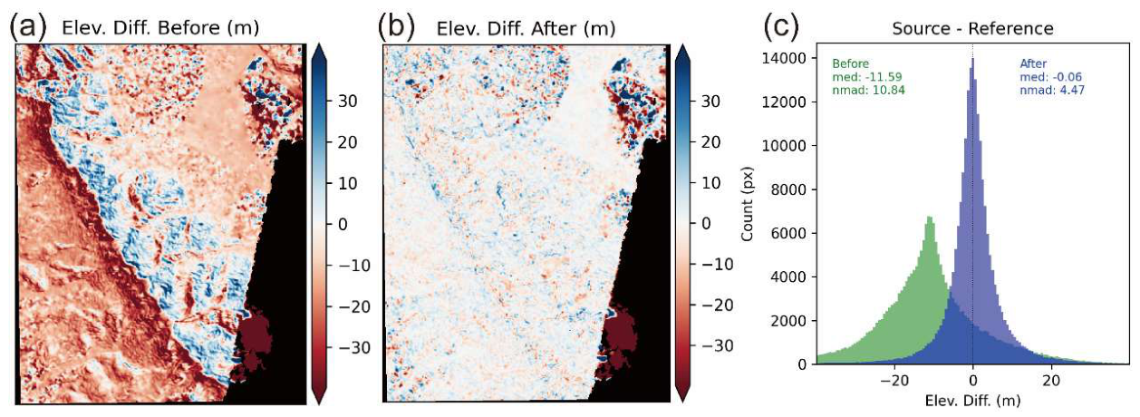
Figure 5.
Mean glacier surface velocity in the Aru region. (a) Surface velocity derived from optical image correlation (1991–2016) (b) Seasonal surface velocity derived from Sentinel-1 SAR offset tracking and optical image correlation (2014–2016). Spatial distribution of glacier surface velocity prior to the 2016 ice avalanche event: 20131201-20141126,20141126-20151231,20151028–20160201,20160201–20160304,20160304–20160421和20160421–20160624.
Figure 5.
Mean glacier surface velocity in the Aru region. (a) Surface velocity derived from optical image correlation (1991–2016) (b) Seasonal surface velocity derived from Sentinel-1 SAR offset tracking and optical image correlation (2014–2016). Spatial distribution of glacier surface velocity prior to the 2016 ice avalanche event: 20131201-20141126,20141126-20151231,20151028–20160201,20160201–20160304,20160304–20160421和20160421–20160624.
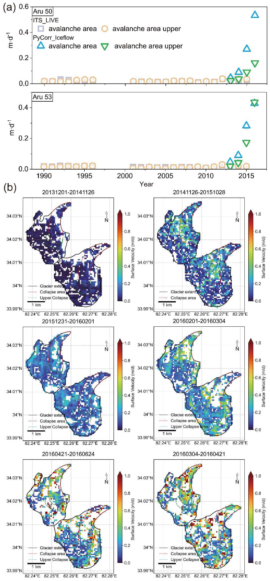
Figure 6.
Pre-collapse surface albedo characteristics of the Aru Glaciers (Aru53 and Aru50) during 1990–2016. The surface albedo analysis included (a) scatter plots illustrating the albedo distribution and (b) annual mean albedo time series for Aru53 and Aru50. (c) Seasonal mean albedo variations during winter (DJF), summer (JJA), and transitional (spring and autumn) seasons.
Figure 6.
Pre-collapse surface albedo characteristics of the Aru Glaciers (Aru53 and Aru50) during 1990–2016. The surface albedo analysis included (a) scatter plots illustrating the albedo distribution and (b) annual mean albedo time series for Aru53 and Aru50. (c) Seasonal mean albedo variations during winter (DJF), summer (JJA), and transitional (spring and autumn) seasons.
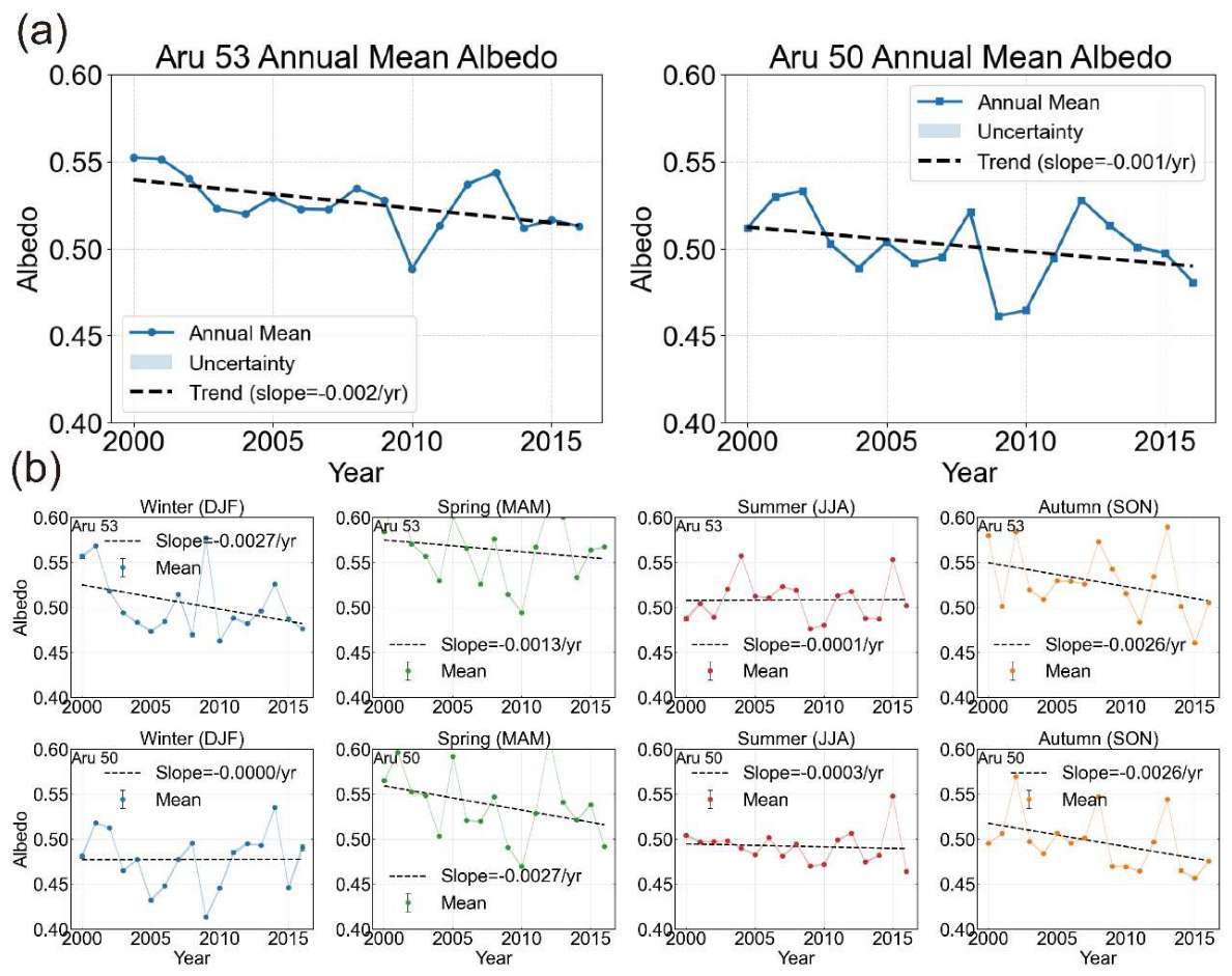
Figure 7.
Pre-collapse surface temperature characteristics of the Aru Glaciers (Aru53 and Aru50) during 1990–2016. (a, b) Surface temperature analysis for Aru53 and Aru50, including scatter plots showing the temperature distribution and annual mean GST time series, respectively. (c) Seasonal mean GST variations during winter (DJF), summer (JJA), and transitional (spring and autumn) seasons.
Figure 7.
Pre-collapse surface temperature characteristics of the Aru Glaciers (Aru53 and Aru50) during 1990–2016. (a, b) Surface temperature analysis for Aru53 and Aru50, including scatter plots showing the temperature distribution and annual mean GST time series, respectively. (c) Seasonal mean GST variations during winter (DJF), summer (JJA), and transitional (spring and autumn) seasons.
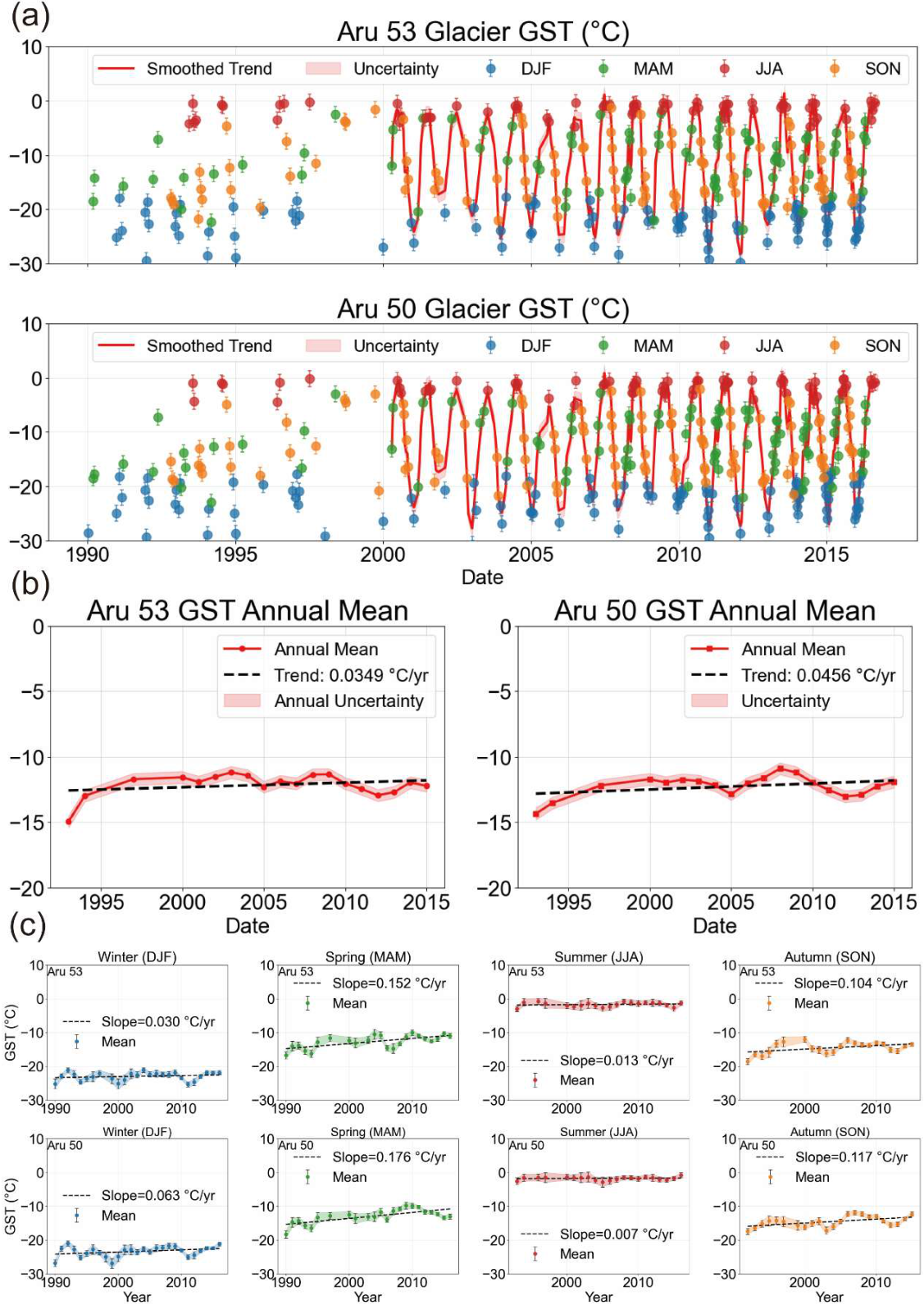
Figure 8.
(a–b) Temporal evolution of the spatially averaged surface backscatter coefficient (σ⁰) for the Aru 53 and Aru 50 glaciers from 2014 to 2016 (the cold seasons, December -April). (c–h) Optical satellite images acquired on November 26, 2014, October 28, 2015, and June 24, 2016, showing the pre-collapse conditions of the Aru glaciers. Black arrows indicate developing crevasses prior to failure, and red arrows highlight the rupture zones. Horizontal arrows denote the inferred position of the head scarp after the failure. (i) Spatial distribution of the temporal trend (slope k) of the backscatter coefficient (σ⁰) across the Aru Glacier region, along with representative σ⁰ intensity maps. (j) Temporal trend (slope k) of σ⁰ for 28 surrounding glaciers. (k) σ⁰ intensity maps of the Aru 53 Glacier on December 27, 2014, December 22, 2015, and May 14, 2016. (l) σ⁰ intensity maps of the Aru 50 Glacier on December 27, 2014, September 17, 2015, and September 11, 2016.
Figure 8.
(a–b) Temporal evolution of the spatially averaged surface backscatter coefficient (σ⁰) for the Aru 53 and Aru 50 glaciers from 2014 to 2016 (the cold seasons, December -April). (c–h) Optical satellite images acquired on November 26, 2014, October 28, 2015, and June 24, 2016, showing the pre-collapse conditions of the Aru glaciers. Black arrows indicate developing crevasses prior to failure, and red arrows highlight the rupture zones. Horizontal arrows denote the inferred position of the head scarp after the failure. (i) Spatial distribution of the temporal trend (slope k) of the backscatter coefficient (σ⁰) across the Aru Glacier region, along with representative σ⁰ intensity maps. (j) Temporal trend (slope k) of σ⁰ for 28 surrounding glaciers. (k) σ⁰ intensity maps of the Aru 53 Glacier on December 27, 2014, December 22, 2015, and May 14, 2016. (l) σ⁰ intensity maps of the Aru 50 Glacier on December 27, 2014, September 17, 2015, and September 11, 2016.
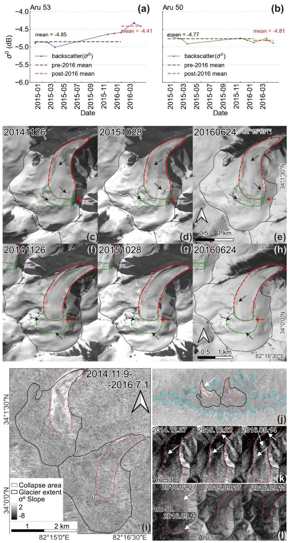
Figure 9.
Multi-parameter evolution of the Aru glaciers prior to collapse (1990–2016), showing the normalized time series of four key pre-collapse indicators: surface velocity, surface elevation change, surface temperature, and surface albedo.
Figure 9.
Multi-parameter evolution of the Aru glaciers prior to collapse (1990–2016), showing the normalized time series of four key pre-collapse indicators: surface velocity, surface elevation change, surface temperature, and surface albedo.
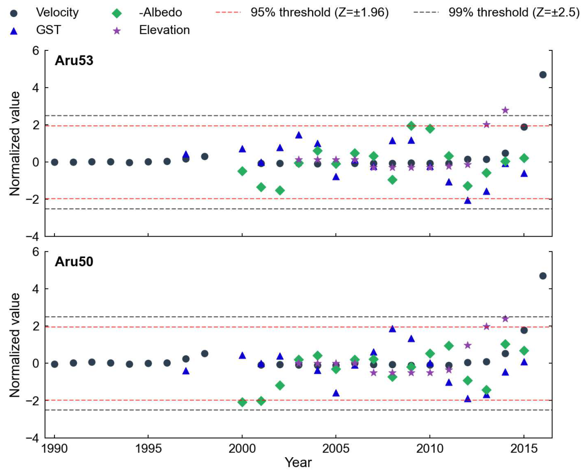

Table 1.
Details of data products used in this study.
| Indicators | Dataset | Spatial resolution | Temporal coverage | Source |
|---|---|---|---|---|
| Elevation | ASTER | 30 m | 2003-2015 | NASA ASTER GDEM |
| Glacier boundary | RGI 7.0 | - | 2000-2020 | Randolph Glacier Inventory 7.0 |
| Glacier boundary | Landsat (TM/ETM+/OLI) | 30 m | 1991-2016 | USGS Earth Explorer |
| Surface temperature | Landsat Collection 2 Level-2 Surface Temperature (ST) | 30 m | 1997–2015 | USGS via Google Earth Engine |
| Surface Backscattering coefficient | Sentinel-1 GRD | 15 m | 2014-2016 (December to April) |
Copernicus Open Access Hub |
| Surface albedo | MODIS MCD43A3 V6.1 | 500 m | 2000-2015 | NASA LP DAAC |
| Surface velocity | ITS_LIVE Glacier Velocity | 120 m | 1990–2015 | NASA Jet Propulsion Laboratory (JPL) |
| Meteorological data | ERA5 reanalysis | 0.25° | 1990-2016 | Copernicus Climate Data Store |
| Meteorological data | GPM IMERG | 0.1° | 2016.01-2016.10 | NASA GPM Mission(NASA/JAXA) |
Notes: DEM, Digital Elevation Model; RGI, Randolph Glacier Inventory; TM, Thematic Mapper; ETM+, Enhanced Thematic Mapper Plus; OLI, Operational Land Imager; GRD, Ground Range Detected; MODIS, Moderate Resolution Imaging Spectroradiometer; ERA5, ECMWF Reanalysis v5; GPM IMERG, Integrated Multi-satellite Retrievals for Global Precipitation Measurement.
Disclaimer/Publisher’s Note: The statements, opinions and data contained in all publications are solely those of the individual author(s) and contributor(s) and not of MDPI and/or the editor(s). MDPI and/or the editor(s) disclaim responsibility for any injury to people or property resulting from any ideas, methods, instructions or products referred to in the content. |
© 2026 by the authors. Licensee MDPI, Basel, Switzerland. This article is an open access article distributed under the terms and conditions of the Creative Commons Attribution (CC BY) license (http://creativecommons.org/licenses/by/4.0/).
Copyright: This open access article is published under a Creative Commons CC BY 4.0 license, which permit the free download, distribution, and reuse, provided that the author and preprint are cited in any reuse.