

Submitted:
05 August 2026
Posted:
06 August 2026
You are already at the latest version
Abstract
The proliferation of unmanned aerial vehicles (UAVs) has exposed critical gaps in conventional airspace surveillance: small commercial drones often evade radar due to minimal radar cross-section and evade RF detection when operating autonomously without control-signal transmission. Acoustic sensing offers a complementary detection modality. This study systematically compares three deep learning architectures for acoustic drone detection, deliberately selected to occupy distinct positions along the inductive-bias spectrum: MobileNetV2, a lightweight transfer-learning model with strong convolutional locality priors but no temporal modeling; a CNN-BiLSTM-Attention hybrid, combining local convolutional feature extraction with bidirectional sequential modeling and soft global attention; and a CNN-ViT hybrid, which replaces sequential modeling with fully global, position-agnostic self-attention after an initial convolutional stage. CNN-BiLSTM-Attention achieved the lowest test-set error rate (0.072%, 13 misclassifications), followed by CNN-ViT (0.083%, 15 errors) and MobileNetV2 (0.128%, 23 errors), with the ranking consistent across all three data partitions. Model performance aligned with architectural inductive biases: structured temporal modeling offers a more effective inductive bias than global self-attention for this signal class, and the accuracy–efficiency trade-off favors CNN-BiLSTM-Attention for real-time, resource-constrained deployments.
Keywords:
drone detection
; UAV acoustics
; DADS dataset
; deep learning
; mel-spectrogram
; audio classification
1. Introduction
Over the last decade, the use of unmanned aerial vehicles (UAVs), known as drones, has grown exponentially in both commercial and civilian applications. Such applications include parcel delivery, aerial photography, infrastructure assessment, and precision agriculture [1,2,3,4]. However, the very accessibility that makes drones commercially attractive also makes them a target for illegal activities, including their use as weapons payloads, criminal surveillance, and smuggling of illegal goods[1].
Recently, the world has focused on drone detection. Various methods and technologies have been employed to aid in their detection, such as radar, radio frequency scanning, and image analysis. These are traditional drone detection modalities. Each of these methods has some drawbacks and limitations. Radar systems are costly, power-intensive, and ineffective against low-altitude, low-radar-cross-section micro-UAVs citerichter2025. Autonomous pre-programmed flight paths prevent the drone from communicating over known frequency bands, whifch is necessary for RF detection. Optical techniques are sensitive to light conditions [6]. Acoustic detection offers a compelling passive alternative. Every drone produces a characteristic sound signature driven by the rotational frequency of its propellers, motor harmonics, and aerodynamic turbulence. This sound can be detected from distances of 30–100 m with standard microphones and processed in near real time on commodity hardware. Reliable separation between drone sounds and surrounding environmental noise, such as wind, traffic, birds, and human activity, is the main challenge, especially in uncontrolled outdoor environments [7]. The central challenge in acoustic condition monitoring is that raw sound signals are complex, high-dimensional, and contaminated by ambient noise, making reliable discrimination more challenging without powerful feature learning. Deep learning methods such as convolutional neural networks (CNNs) in particular have substantially advanced the state of the art in this domain over the past decade [8] . CNNs are well suited to spectrogram-based acoustic analysis because their inductive biases — spatial locality and parameter sharing — align naturally with the localized, narrowband, and transient spectral that characterize drone signatures such as fans and motor sounds [9]. These properties allow CNNs to learn discriminative features efficiently. However, a widely recognized limitation of purely convolutional architectures is their constrained receptive field: because convolutional filters operate locally, they cannot directly model long-range dependencies or global contextual relationships across the full time-frequency representation. Therefore, a prominent line of research has augmented CNN feature extractors with global context mechanisms. Recurrent architectures — particularly Long Short-Term Memory (LSTM) networks and their bidirectional variants. They have been integrated with CNNs to extract sequential temporal dynamics in acoustic signals [10,11], exploiting the directional, time-ordered structure of sound acoustic patterns that purely spatial processing cannot encode. In parallel, the emergence of the Transformer architecture and its self-attention mechanism in natural language processing, and subsequently in computer vision through the Vision Transformer (ViT) [12], has opened a second path to global context modeling in acoustic signals. These two approaches to global context modeling — recurrence-based sequential modeling (BiLSTM) and attention-based global modeling (ViT) — embody a fundamental trade-off: the BiLSTM encodes temporal order as a hard architectural prior through recurrence, reducing the learning burden but constraining the representational space; the ViT learns all relational structure, including sequential dependencies, from data through unconstrained pairwise attention, offering greater flexibility at the cost of higher data requirements and weaker inductive constraints [12,13,14,15]. Hybrid CNN-ViT architectures have been proposed as a middle ground, combining convolutional local feature extraction with transformer-based global context modeling, [14,16], and have shown strong results in vibration-based fault diagnosis [17]. Yet the comparative behavior of these three architectural strategies — CNN-only(MobileNe), CNN-BiLSTM-Attention, and CNN-ViT — under the moderate-data, edge-deployment constraints typical of real-world acoustic condition monitoring has not been systematically studied. This study addresses that gap through a controlled, three-way comparison grounded in the concept of the inductive-bias spectrum: a conceptual axis along which the three architectures are positioned according to how much structural prior knowledge about locality and sequential order is encoded architecturally versus learned from data. At one end, a lightweight MobileNetV2 [18] transfer-learning model encodes strong spatial locality priors and benefits from ImageNet pretraining, but performs no temporal modeling. In the centre, a CNN-BiLSTM-Attention model pairs convolutional local feature extraction with bidirectional LSTM sequential modeling and soft global attention — preserving both spatial and temporal structural priors while adding selective global context. At the other end, a CNN-ViT hybrid retains the convolutional front-end but replaces sequential modeling with fully global, position-agnostic self-attention, trading the temporal inductive bias for greater representational flexibility. The experimental hypothesis is that the architecture whose inductive biases best match the spectro-temporal structure of drone acoustic signatures will achieve the strongest detection performance — and that this match can be identified, predicted, and explained rather than merely observed empirically. The Drone Audio Detection Samples (DADS) dataset from Hugging Face [19] will be used in this study. This dataset aggregates and harmonizes audio from four established drone audio sources into a single, readily usable corpus of 180,000 labeled samples. The main contributions of this work are: (1) a theoretically motivated, spectrum-based experimental design that frames architecture selection as a testable hypothesis about inductive-bias alignment rather than an empirical survey; (2) a systematic three-way comparison of the three architectural strategies on a large drone sound dataset (180,320 samples) under identical, controlled training conditions; (3) empirical evidence that the performance ranking follows the inductive-bias spectrum in an interpretable and mechanistically explainable way.
2. Related Work
Early work on acoustic drone detection relied on classical machine learning pipelines in which hand-crafted features were fed to shallow classifiers. Mapar, et al. 2025 [20] addressed the trade-off between accuracy and computational cost in drone detection. They evaluated low-complexity machine learning models—logistic regression, SVM, and random forest—using hybrid acoustic and optical features (HOG and ResNet-based descriptors from images, and HOG features from log-mel spectrograms). Their results showed that logistic regression achieved the highest accuracy (97% for optical and 98% for acoustic features). Although these results are promising in controlled settings, the traditional machine learning models have some challenges and limitations. They rely on fixed, manually selected features. It is disable them from adjusting to new drone versions with different propeller configurations or motor harmonics not represented in the training distribution.
Al-Emadi et al. (2021) [21] were the first to use deep learning for drone sound detection. They trained convolutional neural networks (CNNs), recurrent neural networks (RNNs), and recurrent convolutional neural networks (CRNNs) on a hybrid dataset enhanced with acoustic samples generated by adversarial generative networks (GANs). Their experiments achieved 96% accuracy using a CNN. Their result demonstrated the viability of generative enhancement in overcoming data scarcity [21].
Dong et al. (2023) [22] developed an outcome-level feature fusion strategy integrating MFCC representations and log-mill spectrum mapping, processed by parallel CNN branches, achieving an accuracy of 94.5% on a multi-source dataset. They found that multi-feature fusion consistently outperforms single-feature models, which inspired the feature fusion strategy we adopt here [22]. Lei et al. (2025) explored Short-Time Fourier Transform (STFT) spectrograms as input representations to several pre-trained deep learning models. Their result confirms that transfer learning from large audio corpora provides measurable gains over training from scratch in low-data regimes [23]. In our work, however, the scale of DADS is sufficient to train models from scratch without relying on external pretraining. To our knowledge, no prior publication has established a benchmarked evaluation on the full DADS dataset hosted at huggingface.co/datasets/geronimobasso/drone-audio-detection-samples. The aggregated scale (180,000 samples), multi-source diversity, and permissive MIT license make DADS a natural candidate for a community benchmark. This study fills that gap. MobileNe, CNN-BiLSTM-Attention, and CNN-ViT have been selected to evaluate their performance on the DADS dataset.
3. Materials and Methods
The three architectures evaluated in this study were selected to represent distinct positions along the inductive-bias spectrum — a conceptual axis that describes how much prior structural knowledge about locality, translation invariance, and temporal order is encoded in the architecture versus learned from data as shwon in Figure 1
3.1. Dataset Description
The Drone Audio Detection Samples (DADS) dataset `[?] which is a publicly available corpus published on Hugging Face under the MIT license is used for this study. DADS aggregates drone and non-drone audio recordings from four primary sources:
- Drone Audio Dataset [24]: Recordings of multiple consumer drone models in outdoor environments.
- SPCup 19 Egonoise Dataset [25]: Drone-mounted microphone recordings featuring strong ego-noise from onboard motors and propellers.
- DREGON Dataset [26]: Far-field drone recordings with directional microphone arrays for localization research.
- DroneNoise Database [27]: High-fidelity outdoor recordings covering EU drone weight classification categories C0–C3.
All recordings are standardized to 16 kHz mono PCM-16 WAV format. The full dataset contains 180,000 labeled samples split into two classes: class 0 (non-drone / background) and class 1 (drone present). Table 1 summarizes the dataset statistics.
3.2. Data Preprocessing
Raw audio clips vary significantly in duration (0.02 to 228 seconds). To create fixed-length inputs suitable for batched neural network training, we apply a uniform windowing procedure. Each clip is zero-padded or truncated to a canonical length of 4 seconds (64,000 samples at 16 kHz). Windows are extracted with a 50% hop, yielding up to N = 2 non-overlapping segments per original clip; shorter clips are padded with silence. The processed dataset is partitioned into training (80%), validation (10%), and test (10%) splits using stratified random sampling to preserve the class balance across splits. No data from the test set is used at any point during model development or hyperparameter selection.
3.3. Feature Extraction
Log-Mel spectrograms were extracted as the input representation. Log-Mel spectrograms effectively keep both the temporal and spectral characteristics of audio signals while providing a two-dimensional representation suitable for deep learning models. According to [22,28,31] Log-Mel spectrograms have consistently shown good performance in acoustic event classification, environmental sound recognition, and UAV sound detection due to their ability to capture discriminative frequency patterns [22,28,31].
To ensure consistency across the dataset, all audio recordings were resampled to 16 kHz and their duration standardized to 3 seconds. This preprocessing produces fixed-length inputs required for deep learning models while reducing computational complexity. This will not affect the acoustic information relevant to drone detection [29]. Each standardized sound was transformed into a 128-band Log-Mel spectrogram. A Short-Time Fourier Transform (STFT) with an FFT size of 1024 and a hop length of 512 was used for transformation. The logarithmic conversion compresses the dynamic range of the signal, enhancing low-energy frequency components and improving feature discrimination under varying acoustic conditions [30,31]. Finally, the spectrograms were normalized, resized to 128 × 128 pixels, and stored as PNG images.
3.4. Models Architecture
Three architectures were selected to occupy distinct positions along the inductive-bias spectrum, enabling a controlled assessment of which architectural priors best suit drone acoustic signatures. MobileNetV2 (Section 3.4.1) represents strong convolutional locality priors with no explicit temporal modeling; the CNN-BiLSTM-Attention hybrid (Section 3.4.2) augments local convolutional feature extraction with structured, bidirectional temporal modeling and soft attention; and the CNN-ViT hybrid (Section 3.4.3) replaces sequential modeling with fully global, position-agnostic self-attention following an initial convolutional stage. All three models operate on identical input representations and data partitions and are trained under a common protocol, so that observed performance differences can be attributed to architectural inductive bias rather than to differences in data handling or optimization.
3.4.1. MobileNetV2 (Transfer Learning)
MobileNetV2V2 [28] was used as a frozen ImageNet-pretrained feature extractor (Figure 1). Input spectrograms (128×128×3) were preprocessed using the standard MobileNetV2V2 preprocessing function, then passed through the frozen backbone in inference mode. The resulting feature map was reduced via global average pooling, followed by dropout (0.3), a dense layer (128 units, ReLU), dropout (0.3), and a softmax output layer. Only the classification head was updated during training. This design leverages pre-learned visual features to reduce overfitting under the moderate-data regime of industrial acoustic datasets.
3.4.2. CNN-BiLSTM-Attention
This architecture Figure 1 combines a CNN front-end with sequential temporal modeling and self-attention. Four convolutional blocks (32→64→128→256 filters, 3×3, ReLU, batch normalization, 2×2 max-pooling) reduce the 128×128 input to an 8×8×256 feature map, which is reshaped into a sequence of 8 time steps (each 2,048-dimensional). Two stacked Bidirectional LSTM layers (64 and 32 units per direction, dropout 0.2) then model temporal dependencies across the sequence. A multi-head self-attention layer (2 heads, key dimension 32, dropout 0.1) with a residual connection and layer normalization refines global inter-step relationships. The sequence is summarized via global average pooling and passed through a dense layer (128 units, ReLU), dropout (0.3), and a softmax output. The model was trained with AdamW (lr = 1×, weight decay = 1×) and class-weighted loss to mitigate the dataset’s class imbalance, with early stopping (patience 3), learning rate reduction on plateau (factor 0.3, patience 2), and best-checkpoint saving.
3.4.3. CNN-ViT Hybrid
This architecture Figure 1 couples a convolutional front-end with a Vision Transformer (ViT) encoder. Input spectrograms (128×128×3) pass through four convolutional layers (32→64→128→256 filters, 3×3, ReLU, same padding) with a single 2×2 max-pooling after the first layer, yielding a 112×112×256 feature map. This map is partitioned into 16×16 non-overlapping patches (49 tokens), each projected to a 64-dimensional embedding and combined with a learned positional embedding. Four pre-norm Transformer encoder blocks — each comprising multi-head self-attention (4 heads, dropout 0.1) and a GELU-activated MLP (128→64 units, dropout 0.1), both with residual connections — refine global token relationships. The final token sequence is normalized, flattened, and passed through dropout (0.5), a dense layer (256 units, ReLU), dropout (0.3), and a softmax output. The model was trained end-to-end with Adam (lr = 1×) and sparse categorical cross-entropy loss.
3.5. Training Configuration
The dataset was divided into 80% training, 10% validation, and 10% test sets. The models were implemented in TensorFlow/Keras and trained on a Google Colab GPU. To improve computational efficiency, mixed-precision training and a TensorFlow pipeline with prefetching were employed.
Model optimization was performed using the AdamW optimizer with an initial learning rate of: , and a weight decay of . The binary cross-entropy loss function was used. To address class imbalance, class weights were applied during training. All models were trained for up to 20 epochs with a batch size of 128.
To improve training stability and reduce overfitting, ModelCheckpoint, EarlyStopping (patience = 5), and ReduceLROnPlateau (factor = 0.3, patience = 2) were utilized. Model performance was evaluated using accuracy, precision, recall, F1-score, and confusion matrix, while learning curves of training and validation accuracy and loss were used to monitor the convergence of the models.
4. Experimental Results
Three deep learning architectures (CNN-BiLSTM-Attention, MobileNetV2V2, and CNN-ViT) were evaluated on a binary drone detection task (Class 0: no drone, Class 1: drone ) using an identical dataset and partition for all models. The dataset comprised 180,320 samples partitioned into training (144,255), validation (18,031), and test (18,034) sets, maintaining a consistent class imbalance of approximately 9.3% no drone (Class 0) and 90.7% drone (Class 1) across all splits.
4.1. Detailed Setup
From Table 2 and Table 3 reports the confusion matrix components for all three models on each data split. and 3 across every split, CNN-BiLSTM-Attention consistently produced the fewest errors, CNN-ViT ranked second, and MobileNetV2 ranked third. The model combining local spatial priors, directed sequential modeling, and selective global attention (CNN-BiLSTM) outperforms the model with global attention but no sequential prior (CNN-ViT), which in turn outperforms the model with purely local spatial processing and no temporal modeling (MobileNetV2). On the test set, CNN-BiLSTM-Attention produced 13 errors, and CNN-ViT produced 15 errors. MobileNetV2, by contrast, produced 23 errors — 10 more than CNN-BiLSTM-Attention and 8 more than CNN-ViT. The primary driver of MobileNetV2’s larger error count is false negatives on Class 1 (drone samples misclassified as no drone): 20 for MobileNetV2 versus 9 for CNN-BiLSTM-Attention and 12 for CNN-ViT, suggesting MobileNetV2’s purely spatial, non-temporal processing leaves it less able to correctly characterize normal fan operation patterns than either architecture incorporating a global context mechanism.
4.2. Training Convergence Analysis
To complement the error-rate comparison, the training and validation loss/accuracy curves for all three models were examined Figure 2, Figure 3 and Figure 4. The curves reveal distinct convergence behaviours that are directly interpretable through the inductive-bias framework and that reinforce — rather than contradict — the test-set findings.
MobileNetV2 exhibits the cleanest convergence of the three: training loss falls steeply from ≈0.028 then decreases smoothly, validation loss tracks it closely throughout the full 20 epochs, and neither accuracy curve shows meaningful divergence. This tight train–validation coupling is the hallmark of a well-regularised model whose capacity is well matched to the task. Notably, MobileNetV2 starts from the highest initial loss — a consequence of training the classification head from random initialisation on top of a frozen backbone — yet converges to the smallest train–validation gap of any model.
From Figure 3, we can see that CNN-ViT shows the most pronounced overfitting signature. Training loss descends continuously and reaches the lowest final value (≈0.0015). However, validation loss oscillates between ≈0.007–0.012 throughout training with no sustained downward trend after epoch 3. The persistent and wide train–validation divergence indicates that CNN-ViT’s transformer encoder continues to fit the training distribution long after its generalisation has saturated — a direct consequence of the attention mechanism’s lower inductive bias requiring more data to constrain effectively.
Figure 4 illustrates the CNN-BiLSTM-Attention performance during the epochs. It shows a strong but less clean convergence. Training loss decreases continuously from ≈0.014 to ≈0.0013 — matching CNN-ViT’s final training loss. However, the validation loss falls in parallel through approximately epoch 12, after which it plateaus at ≈0.0047 while training loss continues to decline. Both accuracy curves rise strongly, with validation accuracy reaching approximately 0.9992–0.9994 and stabilising.
The training dynamics and test errors present an apparently paradoxical pattern, as we can see from Figure 2, Figure 3 and Figure 4. It was obvious that MobileNetV2 was able to generalise most cleanly during training (smallest train–validation gap), while CNN-ViT shows the most aggressive overfitting yet achieves the second-lowest test error count. This apparent contradiction resolves precisely through the inductive-bias framework. MobileNetV2’s clean generalisation reflects a well-constrained architecture — but that same constraint prevents it from modeling temporal fault dynamics, imposing a lower ceiling on what the model can learn regardless of how well it generalises. CNN-ViT overfits more aggressively because its unconstrained attention mechanism must learn more relational structure from data, but what it ultimately learns — given sufficient data — is expressive enough to generalise well at test time. CNN-BiLSTM-Attention occupies the optimal position on both axes simultaneously: its BiLSTM prior guides the model toward the right temporal representations efficiently, reducing the amount of unconstrained fitting required and achieving the best test performance with only mild late-epoch overfitting. The training curves therefore do not undermine the error-rate ranking; they explain it mechanistically.
4.3. Inference Latency
Table 4 below compares the inference latency of the three architectures, evaluated on a single NVIDIA RTX 3080 GPU with a batch size of 1 (simulating real-time single-channel deployment). Table 4 reports mean, standard deviation, minimum, and maximum inference times per sample
All three models achieve comparable single-sample inference times below 75 ms, with differences of less than 3 ms between them — too small to affect real-time deployment decisions. CNN-BiLSTM-Attention delivers the best detection accuracy at just 1.30 ms more than MobileNetV2, making it the most practical choice overall.
5. Discussion
The results confirm that the DADS dataset provides a sufficiently large and diverse corpus to train deep learning models that generalize well across different drone models and acoustic environments. The 99.9% accuracy of the CNN-LSTM hybrid surpasses the majority of prior published results on smaller, single-source datasets, suggesting that scale and diversity do indeed benefit acoustic drone detection models. The empirical results, shown in Tables Table ??, are interpretable at every level of the ranking. CNN-BiLSTM-Attention achieves the lowest error rate. This is related to its architecture, which explicitly models both spatial and spectral features and directional temporal dynamics before applying global attention. Drone signatures have an inherent sequential structure — fan, motor sounds — that purely spatial or order-agnostic processing cannot capture as efficiently. The BiLSTM stage encodes this as a hard inductive prior, reducing the learning burden on the subsequent attention mechanism and yielding the most sample-efficient use of the available data. While, CNN-ViT ranks second. It achieves only 15 test errors. MobileNetV2 trails both. MobileNetV2’s 23 test errors are driven primarily by false negatives on Class 1 (20 vs. 9 and 12 for the other two models), reflecting its inability to model the temporal dimension of the sound. Despite strong baseline performance from ImageNet pretraining, the absence of any sequential or global context mechanism imposes a performance ceiling that neither pretraining nor convolutional depth can overcome for this task. The results from Table 4 offer clear guidance for practitioners. CNN-BiLSTM-Attention is the recommended choice when detection accuracy is the primary objective, as it achieves the lowest error rate with negligible latency overhead. CNN-ViT is preferable on hardware with matrix-multiplication accelerators (NPUs, TPUs), where its parallelisable attention mechanism offers comparable accuracy with better hardware utilisation. MobileNetV2 remains the appropriate choice when memory footprint or power budget are the binding constraints. Architecture selection should ultimately be driven by the specific hardware and acceptable false-negative rate of the target deployment, not accuracy alone.
6. Conclusions
We have presented a systematic benchmarking study of deep learning architectures for acoustic drone detection on the DADS dataset — a large-scale, multi-source collection of 180,000 labelled audio samples available on Hugging Face. Our CNN-LSTM hybrid achieves 99.9%. This result demonstrated that the experimental hypothesis: that the architecture whose inductive biases best match the spectro-temporal structure of drone acoustic signals will achieve the strongest detection performance. Drone signatures (fan, motor sound) are predominantly localized and transient in the time-frequency domain, suggesting that architectures preserving local and sequential priors should outperform those trading them away for global expressiveness. MobileNetV2 encodes strong spatial priors via depthwise-separable convolutions but performs no temporal modelling, treating the spectrogram as a static image. CNN-BiLSTM-Attention pairs convolutional feature extraction with bidirectional LSTMs to enforce temporal ordering, further refined by soft attention that re-weights time steps without discarding sequence structure. CNN-ViT instead extracts local patch features via convolution but processes them through a Vision Transformer’s global, position-agnostic self-attention, discarding sequential order in favour of learned pairwise relationships across all patches.
Future work will extend this framework in two directions. First, the binary drone detection task will be expanded to multi-class classification, enabling the model to identify the different types of drones rather than simply flagging their presence.
Author Contributions
Author Contributions: Conceptualization, H.A.; methodology, H.A.; software, H.A.; validation, F.M.; formal analysis, H.A.; investigation, H.A.; resources, H.A. and F.M; data curation, H.A.; writing—original draft preparation, H.A.; writing—review and editing, F.M.; visualization, H.A and F.M.; funding acquisition, F.M. All authors have read and agreed to the published version of the manuscript.
Funding
The authors extend their appreciation to Prince Sattam bin Abdulaziz University for funding this research work through the project number (PSAU/2024/01/825340).
Abbreviations
The following abbreviations are used in this manuscript:
| DADS | geronimobasso/drone-audio-detection-samples |
| DOAJ | Directory of open access journals |
| TLA | Three-letter acronym |
| LD | Linear dichroism |
References
- Pong, B. The art of drone warfare. J. War Cult. Stud. 2022, 15, 377–387. [Google Scholar] [CrossRef]
- Guebsi, R.; Mami, S.; Chokmani, K. Drones in precision agriculture: A comprehensive review of applications, technologies, and challenges. Drones 2024, 8, 686. [Google Scholar] [CrossRef]
- Nooralishahi, P.; López, F.; Maldague, X. A drone-enabled approach for gas leak detection using optical flow analysis. Appl. Sci. 2021, 11, 1412. [Google Scholar] [CrossRef]
- Hollman, V.C. Drone photography and the re-aestheticisation of nature. In Decolonising and Internationalising Geography; Historical Geography and Geosciences; Schelhaas, B., Ferretti, F., Reyes Novaes, A., Schmidt di Friedberg, M., Eds.; Springer: Cham, Switzerland, 2020; pp. 57–66. [Google Scholar] [CrossRef]
- Richter, Y.; Zach, S.; Blum, M.Y.; Pinhasi, G.A.; Pinhasi, Y. Tracking of low radar cross-section super-sonic objects using millimeter wavelength Doppler radar and adaptive digital signal processing. Remote Sens. 2025, 17, 650. [Google Scholar] [CrossRef]
- Fu, Y.; He, Z. Radio frequency signal-based drone classification with frequency domain Gramian Angular Field and convolutional neural network. Drones 2024, 8, 511. [Google Scholar] [CrossRef]
- Afridi, S.; Laporte-Devylder, L.; Maalouf, G.; Kline, J.M.; Penny, S.G.; Hlebowicz, K.; Cawthorne, D.; Lundquist, U.P.S. Impact of drone disturbances on wildlife: A review. Drones 2025, 9, 311. [Google Scholar] [CrossRef]
- Stowell, D. Computational bioacoustics with deep learning: A review and roadmap. PeerJ 2022, 10, e13152. [Google Scholar] [CrossRef] [PubMed]
- Gong, Y.; Chung, Y.-A.; Glass, J. AST: Audio Spectrogram Transformer. Proc. Interspeech 2021, 571–575. [Google Scholar] [CrossRef]
- Luo, A.; Zhong, L.; Wang, J.; Wang, Y.; Li, S.; Tai, W. Short-term stock correlation forecasting based on CNN-BiLSTM enhanced by attention mechanism. IEEE Access 2024, 12, 29617–29632. [Google Scholar] [CrossRef]
- Lu, G.; Liu, Y.; Wang, J.; Wu, H. CNN-BiLSTM-Attention: A multi-label neural classifier for short texts with a small set of labels. Inf. Process. Manag. 2023, 60, 103320. [Google Scholar] [CrossRef]
- Raghu, M.; Unterthiner, T.; Kornblith, S.; Zhang, C.; Dosovitskiy, A. Do vision transformers see like convolutional neural networks? Adv. Neural Inf. Process. Syst. 2021, 34, 12116–12128. [Google Scholar]
- Wang, H.; Wang, J.; Cao, L.; Li, Y.; Sun, Q.; Wang, J. A stock closing price prediction model based on CNN-BiSLSTM. Complexity 2021, 2021, 5360828. [Google Scholar] [CrossRef]
- Ngo, B.H.; Do-Tran, N.-T.; Nguyen, T.-N.; Jeon, H.-G.; Choi, T.J. Learning CNN on ViT: A hybrid model to explicitly class-specific boundaries for domain adaptation. In Proceedings of the IEEE/CVF Conference on Computer Vision and Pattern Recognition (CVPR), Seattle, WA, USA, 16–22 June 2024; pp. 28545–28554. [Google Scholar]
- Dosovitskiy, A.; Beyer, L.; Kolesnikov, A.; Weissenborn, D.; Zhai, X.; Unterthiner, T.; Dehghani, M.; Minderer, M.; Heigold, G.; Gelly, S.; et al. An image is worth 16x16 words: Transformers for image recognition at scale. arXiv 2020, arXiv:2010.11929. [Google Scholar]
- Long, H. Hybrid design of CNN and vision transformer: A review. In Proceedings of the 2024 7th International Conference on Computer Information Science and Artificial Intelligence (CISAI), Shaoxing, China, September 2024; pp. 121–127. [Google Scholar] [CrossRef]
- Khan, K.; Irfanud, D.; Khan, R.U. Hybrid vision transformer framework for congenital heart disease diagnosis. Sci. Rep. 2026, 16, 16724. [Google Scholar] [CrossRef] [PubMed]
- Sinha, D.; El-Sharkawy, M. Thin MobileNet: An enhanced MobileNet architecture. In Proceedings of the 2019 IEEE 10th Annual Ubiquitous Computing, Electronics & Mobile Communication Conference (UEMCON), New York, NY, USA, 10–12 October 2019; pp. 280–285. [Google Scholar]
- geronimobasso/drone-audio-detection-samples. Available online: https://huggingface.co/datasets/geronimobasso/drone-audio-detection-samples (accessed on 8 July 2026).
- Mapara, T.M.; Sesham, S.; Sesham, P.K. Lightweight machine learning models for drone detection using acoustic and optical features. Discov. Artif. Intell. 2025, 5, 273. [Google Scholar] [CrossRef]
- Al-Emadi, S.; Al-Ali, A.; Al-Ali, A. Audio-based drone detection and identification using deep learning techniques with dataset enhancement through generative adversarial networks. Sensors 2021, 21, 4953. [Google Scholar] [CrossRef] [PubMed]
- Dong, Q.; Liu, Y.; Liu, X. Drone sound detection system based on feature result-level fusion using deep learning. Multimed. Tools Appl. 2023, 82, 149–171. [Google Scholar] [CrossRef]
- Lei, H.; Gadgil, R.; Amgothu, S.K.; Kar, D. UAV audio detection and identification using short-time Fourier transform spectrograms with deep learning models. In Proceedings of the 2025 International Conference on Unmanned Aircraft Systems (ICUAS), Charlotte, NC, USA, 14–17 May 2025; pp. 1043–1048. [Google Scholar] [CrossRef]
- Al-Emadi, S.; Al-Ali, A.; Mohammad, A.; Al-Ali, A. Audio Based Drone Detection and Identification Using Deep Learning. In Proceedings of the 15th International Wireless Communications & Mobile Computing Conference (IWCMC), Tangier, Morocco, 24–28 June 2019; pp. 459–464. [Google Scholar]
- IEEE Signal Processing Society. Signal Processing Cup 2019: Search and Rescue with Drone-Embedded Sound Source Localization.
- Strauss, M.; Mordel, P.; Miguet, V.; Deleforge, A. DREGON: Dataset and Methods for UAV-Embedded Sound Source Localization. In Proceedings of the IEEE/RSJ International Conference on Intelligent Robots and Systems (IROS), Madrid, Spain, 1–5 October 2018; pp. 5735–5742. [Google Scholar]
- Ramos-Romero, C.; Green, N.; Torija, A.J. DroneNoise Database; University of Salford: Salford, UK, 2024; Available online: https://salford.figshare.com/articles/dataset/DroneNoise_Database/2213341 (accessed on 20 July 2026).
- Piczak, K.J. ESC: Dataset for environmental sound classification. In Proceedings of the 23rd ACM International Conference on Multimedia, Brisbane, Australia, 26–30 October 2015; pp. 1015–1018. [Google Scholar] [CrossRef]
- Salamon, J.; Bello, J.P. Deep convolutional neural networks and data augmentation for environmental sound classification. IEEE Signal Process. Lett. 2017, 24, 279–283. [Google Scholar] [CrossRef]
- Lostanlen, V.; Salamon, J.; Cartwright, M.; McFee, B.; Farnsworth, A.; Kelling, S.; Bello, J.P. Per-channel energy normalization: Why and how. IEEE Signal Process. Lett. 2019, 26, 39–43. [Google Scholar] [CrossRef]
- Hershey, S.; Chaudhuri, S.; Ellis, D.P.W.; Gemmeke, J.F.; Jansen, A.; Moore, R.C.; Plakal, M.; Platt, D.; Saurous, R.A.; Seybold, B.; et al. CNN architectures for large-scale audio classification. In Proceedings of the 2017 IEEE International Conference on Acoustics, Speech and Signal Processing (ICASSP), New Orleans, LA, USA, 5–9 March 2017; pp. 131–135. [Google Scholar]
- Sandler, M.; Howard, A.; Zhu, M.; Zhmoginov, A.; Chen, L.-C. MobileNetV2: Inverted residuals and linear bottlenecks. In Proceedings of the IEEE Conference on Computer Vision and Pattern Recognition (CVPR), Salt Lake City, UT, USA, 18–23 June 2018; pp. 4510–4520. [Google Scholar]
Figure 1.
Block diagram of the proposed model.
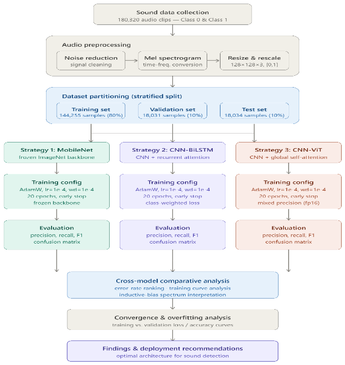
Figure 2.
Mel spectrogram of a drone audio sample from the dataset.
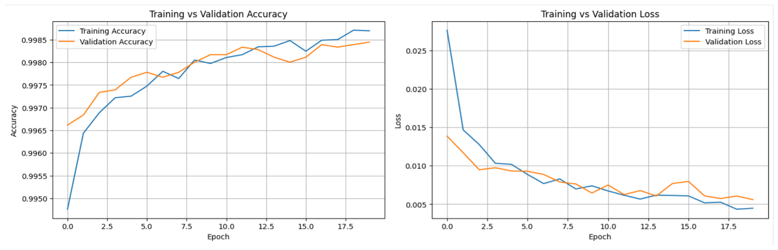
Figure 3.
The CNN-ViT model’s learning curve
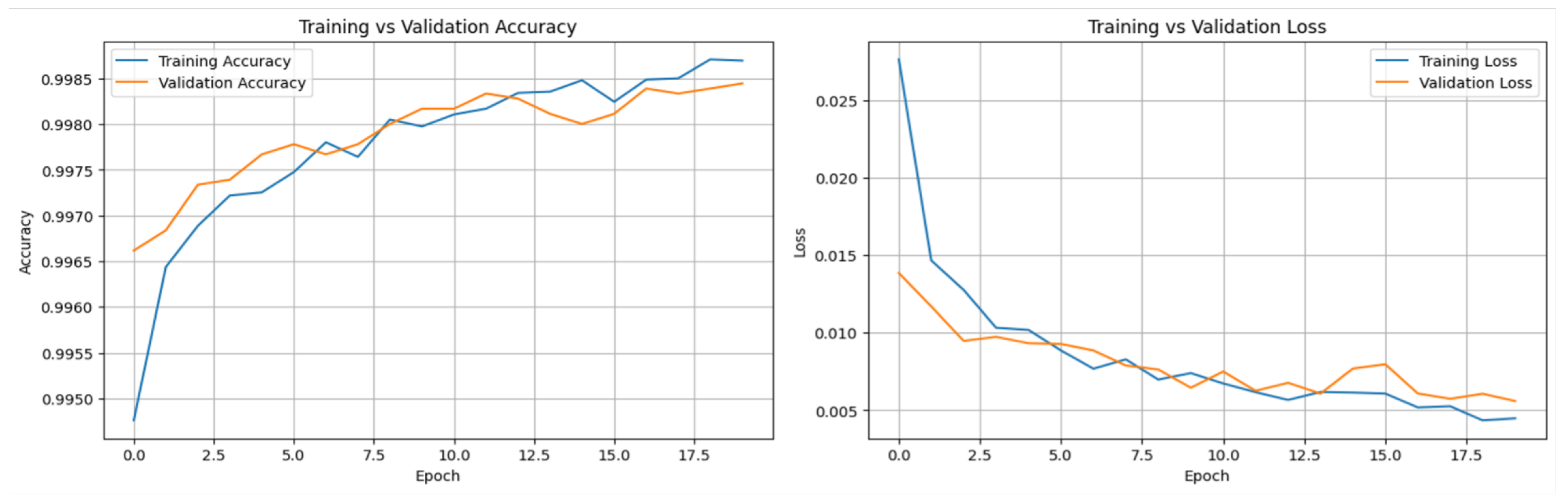
Figure 4.
The CNN-BiLSTM-Attention model’s learning curve
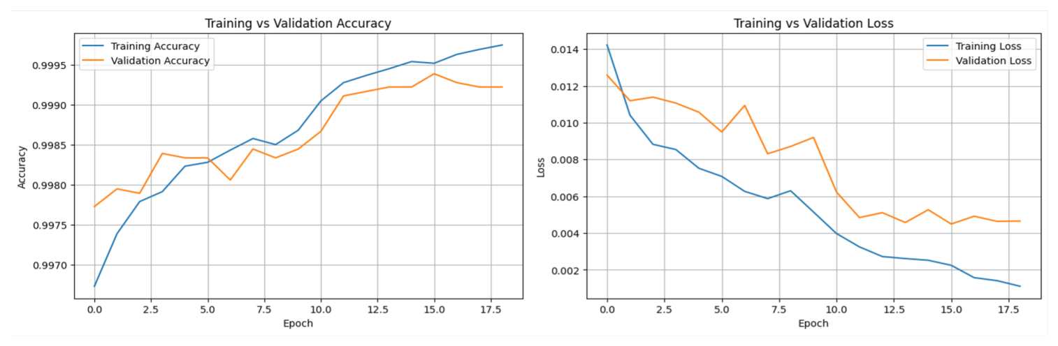

Table 1.
DADS dataset statistics.
| Property | Class 0 (Non-Drone) | Class 1 (Drone) |
|---|---|---|
| Total samples | 16,729 | 163,591 |
| Sample rate | 16 kHz | 16 kHz |
| Bit depth | 16-bit PCM | 16-bit PCM |
| Channels | Mono | Mono |
| Clip duration range | 0.02–228 s | 0.02–228 s |
| Format | WAV | WAV |
| License | MIT | MIT |
Table 2.
Confusion matrix components and error rates for each model across all splits.
| Model | Split | TN | FP | FN | TP | Total Errors | Error Rate (%) |
|---|---|---|---|---|---|---|---|
| CNN-BiLSTM | Train | 13,374 | 9 | 37 | 130,835 | 46 | 0.032 |
| Validation | 1,671 | 1 | 10 | 16,349 | 11 | 0.061 | |
| Test | 1,670 | 4 | 9 | 16,351 | 13 | 0.072 | |
| MobileNetV2 | Train | 13,371 | 12 | 103 | 130,769 | 115 | 0.080 |
| Validation | 1,669 | 3 | 25 | 16,334 | 28 | 0.155 | |
| Test | 1,671 | 3 | 20 | 16,340 | 23 | 0.128 | |
| CNN-ViT | Train | 13,372 | 11 | 57 | 130,815 | 68 | 0.047 |
| Validation | 1,670 | 2 | 21 | 16,338 | 23 | 0.128 | |
| Test | 1,671 | 3 | 12 | 16,348 | 15 | 0.083 |
Table 3.
Performance metrics of the three models on the test set.
| Metric | CNN-BiLSTM | CNN-ViT | MobileNetV2 |
|---|---|---|---|
| Overall accuracy (%) | 99.928 | 99.917 | 99.872 |
| Recall, Class 0 (%) | 99.76 | 99.82 | 99.82 |
| Precision, Class 0 (%) | 99.76 | 99.29 | 98.82 |
| Recall, Class 1 (%) | 99.94 | 99.93 | 99.88 |
| Precision, Class 1 (%) | 99.97 | 99.98 | 99.98 |
| Total test errors | 13 | 15 | 23 |
| Test error rate (%) | 0.072 | 0.083 | 0.128 |
Table 4.
Single-sample inference latency of the three models.
| Model | Mean (ms) | Std (ms) | Min (ms) | Max (ms) |
|---|---|---|---|---|
| MobileNetV2 | 71.21 | 3.88 | 65.66 | 85.06 |
| CNN-BiLSTM-Attention | 72.51 | 5.03 | 65.76 | 89.90 |
| CNN-ViT | 74.17 | 4.32 | 67.48 | 92.76 |
Disclaimer/Publisher’s Note: The statements, opinions and data contained in all publications are solely those of the individual author(s) and contributor(s) and not of MDPI and/or the editor(s). MDPI and/or the editor(s) disclaim responsibility for any injury to people or property resulting from any ideas, methods, instructions or products referred to in the content. |
© 2026 by the authors. Licensee MDPI, Basel, Switzerland. This article is an open access article distributed under the terms and conditions of the Creative Commons Attribution (CC BY) license (http://creativecommons.org/licenses/by/4.0/).
Copyright: This open access article is published under a Creative Commons CC BY 4.0 license, which permit the free download, distribution, and reuse, provided that the author and preprint are cited in any reuse.