

Submitted:
05 August 2026
Posted:
06 August 2026
You are already at the latest version
Abstract
Many practical questions are causal: they ask what would happen to an outcome if we changed a treatment, a price, or a policy. Answering such questions from data requires choosing an estimation method and, before that, deciding whether the question can be answered at all from the available data and assumptions. Both decisions are error prone, and wrong choices can produce answers that look precise while being wrong. We introduce the Causal World Foundation Model (CWFM), a hybrid system in which a neural network, pretrained on a large collection of synthetic causal problems, orchestrates a library of classical causal estimators that are fitted anew to each submitted dataset. Before any estimation, deterministic gates check a declared contract of identification and support conditions. Queries that fail these checks receive a structured refusal with a machine-readable reason instead of a number, and the uncertainty of every answer is calibrated with split conformal prediction. On a locked synthetic benchmark spanning static, randomized, and network-interference settings, CWFM matches the accuracy of the best fixed baseline without knowing which mechanism generated each dataset, keeps its intervals close to the nominal coverage, and refuses every query whose declared conditions fail while the baselines answer all of them. A confirmatory round under a frozen protocol, including a semi-synthetic benchmark built on real energy-sensor covariates, reproduces these findings and sharpens them: all point estimates come from the classical estimator blend, and simple non-neural aggregation baselines match or slightly exceed the pretrained router's accuracy. The demonstrated value of the system therefore lies in the contract, gating, and calibration layer around classical estimation, a practical and transferable role for pretrained causal systems.
Keywords:
causal inference
; trustworthy artificial intelligence
; interpretable artificial intelligence
; foundation models
; estimator selection
; identification
; abstention
; conformal prediction
; network interference
1. Introduction
Many of the most important questions in science, medicine, and industry are causal: they ask what would happen to an outcome if we actively changed something, such as a treatment, a price, a policy, or a process step. Causality is not the same as prediction. A standard machine-learning model answers a different question, namely what is likely to happen if nothing is changed, and it can predict very accurately while being completely wrong about the consequences of an intervention, because prediction exploits every correlation in the data, including correlations that would disappear the moment we intervene [1,2]. A simple example makes the difference concrete. In observational medical data, patients who received an intensive treatment often show worse outcomes than patients who did not, simply because sicker patients are treated more intensively. The data faithfully report this association, yet the treatment may still help every patient who receives it. Predicting outcomes from such data is easy; deciding what would happen if more patients were treated requires separating the effect of the treatment from the effect of being sick in the first place. Answering causal questions therefore requires dedicated methods, and those methods rest on assumptions about how the data were generated.
In practice, causal analysis faces two recurring problems. The first is method choice. Before seeing the answer, the analyst must choose a model class, an estimator, an adjustment strategy, and often more specialized ingredients such as how influence spreads through a network. Each choice is an assumption, and a wrong choice does not merely reduce accuracy; it can produce conclusions that are confidently wrong. Two examples from our own benchmarks illustrate this. When a linear model is fitted to data generated by a single smooth nonlinear mechanism, it can “discover” a change in the causal mechanism that does not exist, while its test loss genuinely improves. And when an unobserved common cause affects both treatment and outcome, a standard estimator can detect an effect in every run while its estimate is severely biased and its confidence interval never contains the truth. In both cases the analysis looks successful by the usual metrics and is wrong precisely where it matters.
The second problem is answerability. Some causal questions cannot be answered from the available data at all: when an unobserved factor drives both the treatment and the outcome, or when the data contain no units comparable to those the question asks about, no method can recover the answer. An honest analysis must recognize such questions and decline them, yet most analysis pipelines and most learned models always return a number. Figure 1 illustrates these failures and the different responses they require.
The state of the art offers two partial answers, each with a gap. On one side, classical causal inference provides a rich theory of identification (determining whether a causal question can be answered at all from the available data and assumptions), together with well-understood estimators [1,2,3]. But every new dataset requires the analyst to select and configure these tools by hand, and the examples above show how easily that selection goes wrong. On the other side, a recent line of work pretrains transformer models on large collections of synthetic causal problems, so that a new dataset can be analyzed without refitting the pretrained network [4,5,6,7]. These causal foundation models remove much of the manual selection burden, and several engage seriously with identification assumptions and uncertainty. Their interfaces, however, typically return an estimate within a causal setting that is assumed by the training prior or supplied by the practitioner; to our knowledge, none exposes a formal, query-level refusal as a first-class output. When the requested quantity is not justified by the supplied assumptions or the data, this design risks automating exactly the false confidence described above. Figure 2 summarizes the two incomplete halves and the combination proposed in this paper.
In this paper we propose the Causal World Foundation Model (CWFM), a hybrid system designed to combine the strengths of both sides and to address the two problems above directly. CWFM contains a transformer pretrained on a large stream of synthetic causal problems. Given a new dataset together with a formally specified causal question, its pretrained parameters stay fixed, while the classical estimators it orchestrates are fitted to each submitted dataset; we use the term foundation model only in this narrow sense of one pretrained checkpoint reused across many datasets and query types. Two design choices distinguish CWFM from prior causal foundation models, one per problem. For method choice, instead of acting as one universal neural estimator, CWFM learns to select and combine a library of well-understood classical estimators, adding a learned correction only where it has not been found to do harm. For answerability, part of the causal setting is externalized as an explicit contract: deterministic identification and data-support checks decide, before any estimate is produced, whether the requested question satisfies the implemented conditions. When it does not, CWFM refuses and states why, instead of returning a misleading number; its uncertainty intervals are calibrated with split conformal methods rather than taken directly from the network.
The contributions of this paper are:
- a structured causal-query and assumption-contract interface, with deterministic identification and support gates that produce explicit, machine-readable refusal reasons for the implemented query classes;
- a pretrained risk router over a library of classical causal estimators, including a cross-fitted doubly robust (AIPW) pathway, with compatibility masking and a gated neural residual, so that one shared checkpoint orchestrates estimation across static, randomized, and network-interference episodes without updating its neural parameters;
- a strictly separated training, calibration, and evaluation protocol measuring accuracy, contract compliance, calibration, structural false positives, and behavior under distribution shift, followed by a protocol-frozen confirmatory round with non-neural aggregation baselines, a gate-compliance property test, a frozen invariance bank, and a semi-synthetic benchmark on real sensor covariates.
As a reproducibility commitment, the model, the synthetic problem generators, and the complete experimental pipeline are openly available.
Our assessment is organized around five research questions:
- RQ1 (accuracy): Can a single pretrained model match well-tuned task-specific estimators on causal questions that are answerable from the data?
- RQ2 (enforcement): Does the runtime gate correctly enforce the declared identification and support requirements, without being bypassed by the learned components?
- RQ3 (structure): Can the system’s calibrated, post-estimation regime diagnostic detect genuine changes in a causal mechanism while rejecting spurious changes induced by model misspecification?
- RQ4 (generalization): How does the model behave on problem families that were held out from its pretraining distribution?
- RQ5 (pathways): Which computational pathways of the architecture actually produce the reported results?
The experimental results can be summarized as follows. On answerable questions, CWFM matches the best single fixed baseline in pooled error without knowing which mechanism generated each dataset, although a correctly chosen per-setting specialist remains somewhat better in individual settings (RQ1). It refuses every query whose declared identification or support conditions fail, while the baselines return a number in all of them (RQ2). Its calibrated regime diagnostic recovers most genuine mechanism changes and, unlike a linear splitting baseline, largely resists splitting a smooth nonlinear mechanism into spurious regimes (RQ3). Accuracy transfers to most problem families excluded from gradient training, with one instructive exception: the family qualitatively unlike the training distribution (RQ4). Finally, the reported estimates are produced entirely by the classical estimator blend selected by the pretrained router; the free-form neural components are inactive at the evaluated checkpoint, which we report openly (RQ5). A protocol-frozen confirmatory round (Section 5.8) reproduces the accuracy, enforcement, and coverage results on fresh episode streams, verifies the repair of an invariance defect found in RQ5, and extends the evidence to a semi-synthetic benchmark on real energy-sensor covariates. It also shows that shallow non-neural aggregation baselines, tuned on a disjoint stream over the same expert library, match or slightly exceed the frozen router’s accuracy.
The remainder of the paper is organized as follows. Section 2 reviews related work. Section 3 introduces the necessary background concepts. Section 4 presents and motivates the CWFM architecture. Section 5 describes the experimental design, answers the five research questions, and reports the confirmatory and external evaluation round. Section 7 discusses implications and limitations, and Section 8 concludes.
2. Related Work
2.1. Formal Identification and Automated Causal-Analysis Systems
Structural causal models and the potential-outcomes framework give causal questions a precise meaning [1,2]. Their central tool is the theory of identification: rules that determine whether a causal question can be answered from the available data under stated assumptions. When point identification fails, sensitivity analysis quantifies how conclusions change as hidden confounding grows [8], partial identification replaces a point estimate with an honest interval [9], and dedicated frameworks cover interference between units [3].
Identification is also an algorithmic problem. The identification algorithm of Shpitser and Pearl gives a complete graphical procedure for identifying arbitrary interventional distributions in semi-Markovian causal models [10]. Building on such results, DoWhy separates modeling, identification, estimation, and refutation [11], DoWhy-GCM exposes a broad family of graphical-causal-model queries through one interface [12], and DECI combines causal discovery and effect inference in a single learned system [13]. Against this background, CWFM’s gate is deliberately narrower: a contract validator that evaluates a finite library of sufficient identification conditions for its three implemented query classes (the randomized ATE, the observational ATE under a declared adjustment set, and network spillovers under a declared exposure mapping), rather than a general engine that derives identifying functionals. The contribution lies in combining this validation with empirical support checks and pretrained estimator routing behind one typed interface.
A complementary classical literature learns causal structure from data, through constraint-based search [14], continuous optimization over graphs [15], invariance across environments [16], heterogeneous and nonstationary data [17], and nonlinear time series [18]. These methods share the burden that motivates amortization: for every new dataset, an expert must choose the algorithm, model class, and tuning parameters without ground truth to check the choice.
2.2. Amortized Causal-Effect Estimation
Prior-data fitted networks (PFNs) amortize inference: a transformer is pretrained on synthetic problems with known ground truth and afterwards processes new datasets without refitting, approximating Bayesian inference under its training prior [19,20]. Its causal instances are the closest comparison group for this paper. CausalFM constructs valid priors for back-door, front-door, and instrumental-variable settings and predicts effects within the setting encoded by the prior [4]; Do-PFN predicts interventional outcome distributions directly from observational data, with no graph required at inference [5]; CausalPFN amortizes average and heterogeneous treatment-effect estimation under ignorability in its prior [21]; and ACTIVA targets full post-intervention distributions given an intervention query [22]. Partial-graph-conditioned models accept causal knowledge as an input rather than fixing it in the prior [23], and temporal and longitudinal variants cover time-series and treatment-sequence data [24,25].
These systems engage seriously with identification, but their published interfaces return an estimate within the assumed or supplied causal setting; none exposes a runtime check, with refusal, that a specific submitted query satisfies explicit identification and support conditions. What is amortized also differs: direct causal PFNs amortize the mapping from a dataset to an effect or interventional distribution, whereas CWFM amortizes the prediction of which per-dataset classical estimators are likely to perform well; indeed its evaluated checkpoint obtains all point estimates from its classical library (Section 5.7). Section 5.3 situates CWFM among these systems at the capability level; published results rest on different benchmarks and estimands, so we make no numerical cross-paper comparison. A related line amortizes causal-structure prediction [6,7,23,26]; graph discovery is relevant to CWFM’s exploratory structural components but is not the evaluated task of this paper.
2.3. Validation, Selection, and Aggregation of Causal Estimators
Causal model selection is difficult because the relevant counterfactual loss is not directly observed. Existing approaches construct proxy validation criteria from influence functions [27], pseudo-outcomes and causal losses such as the R-learner objective [28], counterfactual cross-validation [29], and selective machine learning for doubly robust functionals [30]; empirical studies show that such selection metrics can rank candidate methods unreliably across settings [31,32]. Other work aggregates candidate treatment-effect models instead of selecting one, through ensembles of individualized-treatment-effect estimators [33] and causal Q-aggregation with model-selection guarantees [34], and AutoCATE integrates the entire pipeline for end-to-end automated CATE estimation [35].
CWFM builds on this literature, and its distinguishing element is where the aggregation weights come from. Existing validation and ensemble methods operate within the submitted dataset, because true causal error is unavailable there. CWFM instead trains an episode-level risk predictor across synthetic episodes for which every estimator’s realized error is known, then applies it to new episodes without updating its neural parameters, conditioned on a typed query and only after the contract and support checks have passed. AutoCATE, in particular, performs per-dataset counterfactual pipeline optimization with a much richer CATE search space, whereas CWFM learns one cross-episode router before deployment and places routing behind gates that can withhold the answer entirely. The current estimator library is deliberately small and mechanism-oriented (Section 4.6); extending it with weighting-based, orthogonalized, and forest-based estimators such as TMLE, double machine learning, R-learners, and causal forests is a natural next step.
2.4. Reliability under Non-Identification, Weak Support, and Prior Shift
Positivity and empirical support.
Positivity is a population-level identification condition, whereas overlap diagnostics assess how well it is represented in a finite sample; in high dimensions, empirical overlap can deteriorate rapidly as covariates are added [36]. Existing responses to limited overlap include trimming to a better-supported subpopulation [37], overlap weighting [38], redefining the target population, extrapolation, and partial identification; these are not equivalent to refusal, because trimming and weighting change the target population and therefore the estimand. CWFM is deliberately conservative: when its finite-sample support criterion fails, it refuses the requested estimand rather than silently changing the target population.
Sensitivity analysis and partial identification.
Refusal is not the only defensible output when point identification fails: the appropriate answer can be an identified set [9], a sensitivity curve indexed by an assumed confounding strength [8], or an estimate for a restricted population, and amortized sensitivity analysis makes some of these outputs cheap [39]. CWFM refuses the requested point estimate under the supplied contract; partial-identification outputs are a natural extension.
Prior-induced bias in causal PFNs.
Causal PFNs interpreted as Bayesian ATE estimators can retain prior-induced confounding bias and fail to attain frequentist consistency without correction [40], and a simulation study reports bias and poor credible-interval coverage in clinical-style scenarios [41]. CWFM routes among per-dataset classical estimators rather than treating a PFN posterior as the causal estimate, but it still depends on the synthetic training prior, as the nonmonotone-interference result of Section 5.6 demonstrates.
Conformal calibration and its target.
Conformal prediction provides finite-sample marginal coverage under exchangeability of calibration and future instances [42,43]. The causal-conformal literature targets counterfactual outcomes and individual treatment effects [44], calibration of heterogeneous-effect predictors [45], and intervals under causal-graph uncertainty [46]. CWFM’s guarantee is different in kind: it calibrates scalar episode-level estimation error across exchangeable simulator episodes, so coverage is marginal over the calibration stream’s episode distribution (Section 4.7).
Four meanings of refusal.
Non-answers arise from distinct sources: (i) logical non-identification, where the supplied model and assumptions do not identify the estimand; (ii) finite-sample unsupportedness, where an identified estimand lacks adequate support in the data; (iii) learned high-risk abstention, which trades answer coverage against retained risk [47]; and (iv) out-of-distribution rejection of episodes unlike the training distribution. CWFM’s refusals are deterministic consequences of the declared contract and support policy, cases (i) and (ii); learned reliability heads [48] and self-compatibility checks [49] are complementary layers for cases (iii) and (iv), which CWFM does not yet cover.
Benchmarks that score non-answers.
Recent causal-reasoning benchmarks separate identification from numerical estimation and score whether a system declines underdetermined questions: CausalReasoningBenchmark evaluates identification specifications separately from estimation [50], CausalDS treats abstention as a scored outcome for data-science agents [51], and CausalT5k evaluates structured refusal when evidence is underdetermined [52]. These benchmarks target language models or agents rather than estimator architectures; the shared principle is that non-answer behavior should be evaluated explicitly, which CWFM operationalizes through deterministic statuses.
2.5. Task-Specific Foundations: Interference and Regime Determination
Network interference.
Beyond the classical potential-outcomes treatment of interference [3], design-based frameworks connect the design, the exposure mapping, and the estimand under general interference [53], misspecified exposure mappings have their own estimability theory [54], and machine-learning estimators model network-mediated effects with learned representations [55]. CWFM conditions on a user-supplied network and exposure mapping: its support gate checks whether the requested exposure contrast is represented in the submitted data, but it does not validate the network or the mapping itself, so exposure-mapping misspecification is a separate failure mode from insufficient support.
Regime determination.
What we call regime determination is closest to mechanism-change detection. Model-based recursive partitioning splits a fitted model along covariate thresholds [56] and inspires our splitting baseline, a deliberately compact one-split variant (Section 5.1); causal trees seek subgroups with heterogeneous treatment effects [57]; discovery from nonstationary data exploits mechanism change as a signal [17]; and invariance-based methods test mechanism stability across environments [16]. CWFM’s regime task asks whether the conditional outcome mechanism itself changes at a threshold; its hard negatives distinguish a genuine piecewise mechanism from a smooth nonlinear one that a partitioning method may approximate with multiple regions, since a partition that improves predictive fit is not, by itself, evidence of a regime change.
2.6. Positioning and Research Gap
Each ingredient of CWFM exists in the literature above; the contribution is their integration: for a finite set of implemented query classes, CWFM combines a typed causal query, deterministic validation of a declared assumption contract, an empirical-support policy, a pretrained cross-episode risk router over per-dataset classical estimators, episode-level conformal calibration, and typed non-answer outcomes, with refusal behavior evaluated as a first-class outcome. The contribution is reliability-gated estimator orchestration and its evaluation, not general graphical identification, automatic detection of hidden confounding, or out-of-distribution-safe abstention. Table 1 locates CWFM among representative systems.
3. Preliminaries
This section introduces the four concepts needed to follow the rest of the paper. Readers familiar with causal inference may skip to Section 4.
3.1. Structural Causal Models, Interventions, and Identification
A structural causal model (SCM) describes a system as a set of variables, each generated by a mechanism from its direct causes plus independent noise [1]. As a running example, suppose a variable X (say, the severity of a patient’s condition) influences both a treatment decision A and an outcome Y, and the treatment also influences the outcome. An intervention replaces one mechanism by force: instead of letting doctors choose the treatment, we set it to a fixed value a, written . The canonical causal quantity in this paper is the average treatment effect (ATE),
the expected change in the outcome if everyone were treated versus no one. The difficulty is that we only observe data from the system without the intervention: as in the introduction’s example, sicker patients are treated more often, so naive comparisons mix the effect of the treatment with the effect of severity.
Identification asks whether a causal quantity can, in principle, be computed from the observed data under stated assumptions. In the example, if all common causes of A and Y are observed (here, X), the ATE is identified by the back-door adjustment formula: compare treated and untreated outcomes within each level of X, then average over the population. Estimating this formula by fitting a regression of Y on A and X and averaging its predictions is called g-computation, one of the classical estimators our model builds on. If, however, some common cause is unobserved (hidden confounding), no amount of data from the same source recovers the ATE: the question is not identified, and an honest analysis must say so, widen its answer to a range, or state which additional assumptions would be needed.
3.2. Network Interference and Exposure Mappings
Classical causal inference assumes that treating one unit does not affect another. In many settings this is false: vaccinating my neighbors protects me, and a promotion in one store draws customers from nearby stores. This phenomenon is called interference, and its analysis requires knowing which units are connected, typically as a network [3]. Because a unit can be affected by many neighbors in many ways, one summarizes the treatments of its neighbors by an exposure mapping, for example “the fraction of my neighbors that are treated.” A typical causal quantity is then a spillover effect: the expected change in my outcome if my neighbors’ exposure moved from a low to a high level while my own treatment stayed fixed.
Two conditions matter throughout this paper. First, the exposure mapping is an assumption: if influence depends on, say, edge weights or two-hop neighbors, an analysis based on the simple fraction can be biased. Second, the requested contrast must have overlap (also called positivity): comparable units must be observed at both exposure levels. If nobody in the data ever had a highly treated neighborhood, no method can estimate what would happen in one, and the only correct answer is to refuse.
3.3. Regimes and Mechanism Changes
Real systems are often not governed by one mechanism. The relation between inputs and outcome may differ across subpopulations, for example below and above a threshold of some observed variable: a machine behaves differently past a temperature limit, a subsidy rule changes at an income cutoff. We call such mechanism differences regimes, and regime determination is the task of deciding whether the data were generated by one mechanism or several, and if several, which variable and threshold separate them.
The task hides a trap that plays a central role in this paper. A single smooth nonlinear mechanism can be approximated surprisingly well by two linear pieces, so a procedure that fits linear models and searches for splits will “find” a regime boundary in perfectly stationary nonlinear data, and its predictive accuracy will genuinely improve. The improvement is real; the structural conclusion is false. Regime determination is therefore treated throughout this work as a structural question that requires more than predictive gain.
3.4. Amortized Inference and Conformal Calibration
Traditionally, every new dataset requires selecting and fitting a new statistical model. Amortized inference moves this cost to a single pretraining phase: a neural network is trained on a very large collection of synthetic problems whose true answers are known by construction, and it learns to map a dataset directly to an answer [19]. At deployment, the pretrained network is applied to a new dataset without updating its parameters. Its strength is that it has effectively seen millions of analyses; its weakness is that everything it knows comes from the distribution of synthetic problems it was trained on, which therefore acts as a prior and is part of the model’s assumptions. CWFM adopts the pretraining idea for selection: its neural parameters stay fixed at deployment, but the classical estimators it chooses among are still fitted to each new dataset.
A learned network also outputs uncertainty, but a neural confidence value carries no guarantee. Split-conformal prediction provides one [42,43]. The idea is simple: hold out a set of calibration problems the model has never used for training; record how wrong the model was on each; then widen the model’s intervals on new problems until they cover the observed error distribution at the desired level, for example 90%. Under mild conditions this yields intervals with a finite-sample validity guarantee, which is why all reported uncertainty in this paper comes from conformal calibration rather than from the network’s raw confidence.
4. Approach
CWFM takes a dataset together with a formal causal question and returns either a calibrated causal answer or an explicit, explained refusal. This section presents the architecture step by step. Every component exists to prevent one of the failures described in the introduction, and we state this motivation as each component is introduced.
4.1. Design Principles and Overview
Four principles shape the design.
- 1.
- Amortize the choice of method, not the method itself. The model learns to select and combine well-understood classical estimators; it does not replace them with a free-form neural predictor.
- 2.
- A learned correction must earn its place. A checkpoint is eligible only if its neural correction does not materially degrade the compiled classical estimate on designated development data.
- 3.
- Decide whether the question is answerable before trying to answer it. This decision is made by deterministic logic, not by the network.
- 4.
- Report only uncertainty that carries a guarantee, and refuse rather than guess. Intervals come from conformal calibration; unanswerable questions receive a refusal, never a number.
Figure 3 shows how these principles translate into a pipeline. The input is a causal episode (the data plus everything known about it) together with a formal query that acts as a declared contract (Section 4.2). Before any estimation, two deterministic gates check whether the query satisfies the implemented identification and support conditions; if not, the pipeline exits with a structured refusal (Section 4.5). If the gates pass, a library of classical estimators is fitted to the episode, and a typed encoder with a pretrained risk router blends their candidate estimates into one answer (Section 4.3 and Section 4.6). Conformal calibration then turns the answer into an interval with a stated coverage property (Section 4.7). Two further components, structural world-particle scores and a gated neural residual, are implemented but presently exploratory. Section 4.8 to Section 4.10 describe the training data, the model selection, and what is and is not guaranteed.
4.2. Causal Episodes and the Formal Query Language
The input unit of CWFM is a causal episode: the dataset together with everything relevant that is known about it. An episode contains the observed values, missingness indicators, a schema stating each variable’s type, each variable’s role with respect to the question (treatment, outcome, or covariate), an optional relation matrix connecting the units when interference is possible, and declared design knowledge, for example that the treatment was randomized. Passing this context explicitly matters: whether an analysis is valid often depends less on the numbers than on how they were produced.
The question itself is a formal query: a small structured object stating the claim type (associational or interventional), the treatment and outcome variables, the causal quantity requested (for example the ATE or a spillover contrast), and the target population. We insist on a formal query rather than a natural-language question for two reasons: small changes of wording must not silently change the quantity being estimated, and the claim type prevents a quiet upgrade of an associational finding into a causal one, since an interventional answer can only be produced for a query that requested one and passed the gates. A language model may translate a scientist’s question into this format, but the causal core operates on the structured object only.
Together, the query and the declared design knowledge form a contract, and the whole system is one function
where E is the episode, Q the formal query, and S a status taking one of four values: answer, not identified, unsupported, or out of scope. The point estimate and the calibrated interval are present only when ; R is a machine-readable refusal reason, and D contains diagnostics that carry no guarantee. The three non-answer statuses are deliberately distinct: formally nonidentified under the declared assumptions, identified in principle but outside the implemented rule library, or identified but lacking adequate finite-sample support. Figure 4 makes these objects concrete, and Table 2 lists the implemented query classes.
4.3. Typed Encoder and Mechanism Experts
The encoder converts an episode into internal representations. Each cell of the data table is embedded from its value, its missingness indicator, and its variable’s type and role in the query; there is deliberately no embedding of the column position, because the meaning of a variable should come from its role and type, not from being column four. The query vector does supply the normalized column indices of the treatment, outcome, and exposure variables, so the architecture is best described as
trained under presentation randomization
(Section 4.8) rather than blind to column positions; Section 5.7 measures the consequences.
Attention
is the basic operation of transformer models: each part of the input gathers information from the parts related to it. In CWFM, attention alternates along two axes: across variables within one sample, relating treatment, outcome, and covariates to one another, and across samples within one variable, revealing distributional patterns such as skewness, subgroup structure, or outliers. When the episode contains a relation matrix, an additional message-passing step lets each unit see summaries of its neighbors, as a spillover analysis needs.
The feed-forward layers are organized as a sparse
mixture of mechanism experts. Instead of one universal network, several small expert networks specialize in different mechanism families, and a learned gate activates only the most relevant ones for each episode. We call this the
encoder expert gate, to keep it clearly distinct from the estimator risk router of Section 4.6: the former shapes internal representations, the latter chooses among fitted classical estimators. The gate carries a simplicity prior, so flexible experts are used only when the data demand them: a simple linear method beats a flexible one when the truth is linear and loses when it has a threshold, a distinction that a single uniformly flexible pathway tends to blur.
4.4. Structural Heads and Exploratory World Particles
Structural decoders read the encoder representations and output probabilities rather than hard decisions. The most important one, the
regime decoder, is hierarchical and mirrors how an analyst would reason: is there evidence of a mechanism change; if so, which variable separates the regimes, at which threshold, and what kind of change is it. Because the stationary nonlinear trap of Section 3.3 is the known failure mode, the decoder is trained on matched pairs of episodes in which one curved mechanism and two straight ones look predictively similar but differ structurally. At the evaluated checkpoint, however, the reported regime decision comes not from this learned decoder but from thresholding a compiled, BIC-based evidence statistic against a threshold fitted on the calibration bank (Section 4.7); the decoder’s outputs are recorded as diagnostics only (Figure 5d), which matters for reading Section 5.5.
The architecture also contains
world particles: a small set of scored hypotheses about the data-generating process, each combining a graph, a mechanism family, and a regime hypothesis. The design goal, which gives the model its name, is to separate uncertainty about
which structure
generated the data from uncertainty about
parameters
within a structure. This module is implemented but exploratory: the point estimate does not depend on the particle scores at the evaluated checkpoint, and they remained uninformative in this run (Section 5.7). Figure 5 summarizes the regime pathway.
4.5. Identification and Support Gates
Before any estimate is produced, two gates decide whether the query should be answered at all.
The
identification gate
checks whether the requested causal quantity is identified given the episode’s declared assumptions and design knowledge, for example randomized assignment or that all relevant confounders are observed. This gate is deterministic logic, not a learned component, for a principled reason: identifiability is a property of the causal model and its assumptions and cannot be certified from data patterns alone, so a learned score could only imitate the training prior and would produce exactly the confident wrong answers we aim to prevent; it is the direct response to the hidden-confounding failure of the introduction.
The
support gate
checks whether the requested contrast is present in the data: are there comparable units observed under both treatment values, or both exposure levels, for the population in the query? Two notions must be kept apart:
population positivity, the assumption that the contrast occurs with positive probability in the population, is an identification assumption and belongs to the contract, whereas
observed finite-sample support, which the deployed gate measures, is an empirical statistic of the submitted dataset compared against a threshold. If too few comparable observations exist, any estimate would be extrapolation rather than evidence, and the output is suppressed. One further distinction bounds what the benchmark shows: the public application runtime (Section 6) computes the support statistic from the submitted data, whereas the experiments of Section 5 supply the support condition through the episode’s declared support class, exactly like the identification condition. They therefore measure enforcement of declared conditions; the finite-sample behavior of the empirical support statistic remains to be benchmarked separately.
When a gate fails, CWFM returns a
structured refusal
whose reason code distinguishes the three cases introduced in Section 4.2: formally nonidentified under the declared assumptions, outside the implemented rule library, or inadequately supported in this sample. The refusal also names what would resolve it, for example an instrument, an experiment, or additional data in the unsupported region. Learned diagnostic heads add empirical signals such as estimated overlap and prior mismatch, but they can only add caution, never overrule a gate. Figure 6 shows the decision logic with concrete examples.
4.6. A Risk-Routed Library of Classical Estimators
When both gates pass, the answer is produced by classical statistics guided by the learned model, in three steps.
First, every member of a
library of estimators
compatible with the query class (Table 2) is fitted to the episode’s data, each producing a candidate estimate; incompatible estimators are masked out. Each member is a standard method correct under a different mechanism class: linear g-computation, a cross-fitted augmented-IPW (doubly robust) estimator with ridge-linear nuisance models, g-computation with interactions, a spline-based version, a piecewise (hinge-basis) exposure-response estimator for threshold spillovers, and a design-based estimator for randomized episodes with a null estimator that returns no effect (in the network library, the AIPW slot is a cross-fitted linear plug-in rather than a derived Neyman-orthogonal score). Cross-fitting is used on the nuisance pathways, with cluster-level folds for network episodes. This is genuine per-episode statistical fitting: what stays fixed at deployment are the neural parameters, not the estimators.
Second, the
estimator risk router
predicts, from the episode representation, how large each estimator’s error is likely to be on this episode, and blends the candidates accordingly:
where the weights are obtained from the predicted risks of the compatible estimators. The router is supervised during pretraining: every synthetic episode carries its true effect, so the realized error of every estimator is observable, and the router learns to predict it. We call the
compiled estimate: the answer classical statistics would give if an experienced analyst had chosen and blended the estimators. Figure 7 traces the full computation on a schematic example.
Third, a neural
residual
may adjust the compiled estimate. It is initialized at zero, passes through a learned gate, and is trained with a
no-harm objective
that penalizes any adjustment that worsens the compiled estimate far more than it rewards an improvement; checkpoint eligibility additionally requires that the residual does not materially degrade the compiled estimate on the development banks. If the residual cannot prove its worth, the gate stays closed and the final answer equals the compiled estimate: the burden of proof is on the neural correction, never on the classical estimate (principle 2).
4.7. Calibration
All reported uncertainty comes from split-conformal calibration (Section 3.4): a dedicated bank of calibration episodes, never used for training, records how wrong the model’s answers are in practice, and intervals on new episodes are widened until they cover this error distribution at the target level. The conformal scores are normalized and stratified so that intervals adapt to episode difficulty: an episode routed to a risky estimator, or one where the estimators disagree, receives a wider interval (whether the normalizing scale tracks realized difficulty is exploratory rather than validated). Every baseline is calibrated on the same bank, target, and finite-sample quantile rule, but with ordinary absolute-residual radii rather than CWFM’s normalized score, so the coverage comparison of Section 5 shares the calibration data and target but not the score construction. The threshold at which the regime decision declares a mechanism change is fitted on the same calibration bank rather than learned end to end, for the same reason: a decision with error-rate consequences should be set where its error rate can be measured. On the calibration bank, the fitted threshold attains a false-positive rate of approximately 0.085 with recall maximized among feasible thresholds.
The resulting guarantee is
episode-marginal: over future episodes exchangeable with the calibration stream, the interval contains the true effect with probability at least the nominal level. It is not a conventional confidence interval for one fixed data-generating process under repeated sampling and promises nothing outside the calibration distribution (Section 4.10).
4.8. Training and Evaluation Data
For a pretrained causal model the training distribution is not an implementation detail but part of the model’s assumptions: everything CWFM knows, it knows from this distribution.
All training and evaluation data are
synthetic causal episodes
produced by a simulator, a necessity rather than a convenience: supervising a causal model requires labels that real data cannot provide, namely the true effect of an intervention, the true causal structure, and the true answer to “should this query be refused?”; in a simulation these labels are known by construction. Each episode is created in three steps: a complete causal world is sampled (graph, mechanisms, assignment process, effect size); the world is run to produce an observed dataset; and the ground-truth labels are recorded and hidden from the model.
Episodes come from three task families, matching the implemented scope:
- Static treatment effects: 64 to 128 units with three to eight covariates and a binary treatment affecting a continuous outcome, under linear and nonlinear mechanisms with observed confounding, and randomized experiments.
- Regime determination: five to nine covariates whose outcome mechanism is stationary, splits at a threshold of one covariate (with strong or deliberately weak shifts), or is a stationary smooth nonlinear mechanism, the hard negative of Section 3.3; exact nulls are always included.
- Network interference: units linked by a cluster-structured network and treated cluster by cluster with varying saturation; each unit’s exposure is the treated fraction of its neighbors, and spillover mechanisms are linear, threshold-shaped, or exactly null.
Crucially, every family also generates
unanswerable episodes
in which the correct output is a refusal: hidden confounding (an unobserved variable drives both treatment and outcome) and poor overlap or support (the requested contrast barely occurs in the data). These cases are mixed into training at substantial rates; a model never shown them would learn that answering is always rewarded, precisely the behavior we must avoid.
To prevent superficial shortcuts, the presentation of every training episode is randomized: rows are shuffled, columns are permuted while preserving their declared roles, covariate scales are varied, and a random subset of covariate values (up to five percent) is masked as missing, so the model must rely on the declared roles and types of variables, never on their position or scale.
Training and evaluation use five strictly separated streams with disjoint random-seed ranges, so no episode can appear in more than one stream. Figure 8 shows the generation process, the wall between what the model sees and what only the evaluator sees, and the separation logic of the streams. Training episodes are generated online and never repeated: over 1,600 steps with 24 episodes per batch, the full optimization run consumes 38,400 distinct episodes exactly once each. The final test bank is
locked: evaluated once, after all training, selection, and calibration decisions are frozen, with its 14 scenario cells identical for every method.
The out-of-distribution development bank consists of entire mechanism and graph families excluded from training: hinge, multiplicative, and saturating outcome mechanisms; intercept, variance, and shifted regime changes; two random-network families unlike the cluster networks seen in training; and nonmonotone spillovers. Holding out whole families, rather than new random draws from familiar ones, is what lets Section 5 distinguish genuine generalization from memorization of the training prior.
4.9. Pretraining and Safety-Constrained Model Selection
CWFM is pretrained on the online episode stream of Section 4.8 in stages: the estimator library and router first, with the residual frozen, so that a sound compiled path exists before any neural correction is allowed; then the gated residual under the no-harm objective; and finally joint fine-tuning at a low learning rate.
Model selection enforces the reliability requirements as
eligibility constraints, not as terms in a loss. A checkpoint is eligible only if, on the designated development banks, its residual does not materially degrade the compiled estimate, it keeps the false-regime rate on stationary nonlinear episodes below a cap, and it keeps an acceptable number of estimator experts in active use. Refusal behavior is deliberately not among these criteria: it is enforced at run time by the gates of Section 4.5, which no learned component can bypass, so it holds for every checkpoint. Eligible checkpoints are then ranked by worst-group error on the held-out development families; a more accurate checkpoint that violates any constraint is discarded. This ordering, reliability first and accuracy second, prevents the selection process itself from trading reliability for benchmark scores. In this run the trade-off was real: from step 200 onward, every checkpoint exceeded the 0.30 false-split cap on stationary nonlinear episodes and was rejected, so step 100 was selected although later checkpoints achieved better unconstrained scores (exact per-checkpoint values are in the repository logs).
One consequence of this selection shapes how the results of Section 5 should be read. The selected checkpoint, step 100, lies inside the
first
training stage, saved before the residual-training stage (steps 241 to 1040) and the joint fine-tuning began, so the residual head and the world-effect mixture objective had received no training in the evaluated parameters, which reflect the first 2,400 training episodes. The evaluated system is therefore best interpreted as a pretrained estimator router over a classical library; no claim in this paper concerns a trained residual (Section 5.7).
Finally, the implemented scope: static tabular effects, observed-regime determination, and network interference. Temporal mechanism changes, latent-variable structure, and identification with partially specified graphs are part of the design but not of the evaluated implementation, and no claim in this paper depends on them.
4.10. What Is Guaranteed, and Under Which Conditions
Guarantee, constraint, and calibration name different kinds of properties, and it is easy to overclaim by mixing them up. Table 3 states, for each reliability property of CWFM, what holds, under which conditions, and what is not promised. The most important row is the last: nothing in the current system detects that an episode comes from outside the training prior.
5. Assessment
This section first describes the experimental design, then answers the five research questions of the introduction, one subsection each, adding after RQ1 a contextual comparison with published causal foundation models. Section 5.8 reports a second, protocol-frozen evaluation round on fresh episode streams, and the section closes with qualitative case studies that complement the aggregate metrics with worked examples.
5.1. Experimental Design
All results below come from the locked final test bank of Section 4.8, which is evaluated exactly once, after every training, selection, and calibration decision is frozen. The bank contains 14 scenario cells with 30 seeds each, identical for all methods. Six cells contain answerable effect queries (static linear, static nonlinear, and randomized treatment effects; linear, threshold, and null network spillovers), giving 180 queries with known true effects. Four cells contain regime-determination problems (a strong split, a weak split, the stationary nonlinear hard negative, and a complete null), and the remaining four are
stress cells
with 120 queries that must be refused: hidden confounding and poor overlap in the static setting, hidden confounding and poor support in the network setting.
CWFM is compared against five baselines that always answer: linear g-computation, g-computation with interactions, spline g-computation, a piecewise exposure-response estimator, and random forest g-computation. Each baseline is a representative specialist for at least one implemented mechanism cell, so the comparison is deliberately unfavorable to a general model; random forest g-computation represents a generic flexible fit and is not one of CWFM’s experts, while CWFM’s design-based and null experts are not meaningful stand-alone baselines. For regime determination, the baseline is a compact splitting procedure in the spirit of model-based recursive partitioning [56]: a BIC-penalized linear model with at most one split, called the
one-split linear baseline
throughout (conclusions about it do not extend to richer partitioning methods with nonlinear base models). We also report
CWFM (compiled only), the full system with the neural residual removed; the difference between the two isolates the contribution of the learned correction in RQ5.
One provenance clarification is needed for RQ4: the six held-out families were excluded from all gradient training, but they also form the out-of-distribution development bank used to rank checkpoints (Section 4.8), and the per-family values rest on four episodes per family, so RQ4 is a development diagnostic rather than confirmatory evidence. The implementation is modest: hidden dimension 96, three attention blocks, four mechanism experts, six library members, and about half an hour of training on one GPU.
Metrics are the mean absolute error (MAE) of the estimated effect against the known truth, the empirical coverage and width of the 90% intervals, the rate of false answers on the stress cells, and structure accuracy for regime determination (the method must select the correct split variable, or correctly select no split; threshold localization is not scored). Differences between methods are assessed with paired bootstrap confidence intervals over the shared seeds, and all seeds, configuration values, and package versions are recorded in a result manifest with a cryptographic hash of the evaluated checkpoint, so the experiment can be reproduced exactly.
5.2. RQ1: Accuracy on Answerable Queries
Answer: as a pooled generalist, yes. CWFM matches the best single fixed baseline without knowing which setting it is in and clearly outperforms the generic flexible baseline; a per-cell oracle of specialists remains ahead.
Figure 9 shows the pooled picture over the 180 answerable queries. CWFM reaches a pooled MAE of 0.166, side by side with the two best fixed baselines (interaction g-computation at 0.167, linear g-computation at 0.169) and far ahead of random forest g-computation at 0.329. The paired intervals versus the two best baselines contain zero ( with 95% bootstrap interval versus linear, with versus interaction), while versus random forest the difference is a clear with . Pooled coverage of the 90% intervals is 0.906, with mean width (0.793) in the range of the fixed baselines (0.772 to 0.817) and far below random forest (1.337). The pooled coverage hides heterogeneity: by cell, coverage lies between 0.900 and 0.967 except in the network-threshold cell, which reaches only 0.700 (21 of 30; 95% Wilson interval 0.52 to 0.83), exactly where routing is weakest (Section 5.7). The conformal guarantee is episode-marginal and promises nothing per cell, but the undercoverage should be reported rather than averaged away; per-cell calibration is an evident next step.
The pooled numbers hide the more interesting pattern, shown in Table 4: every specialist wins the cell its assumptions were designed for and loses elsewhere, while CWFM is never the single best method in a cell but is close to the winner in most cells. A
per-cell oracle
that always picks the best method of Table 4 quantifies the remaining gap: its mean over the six cells is about 0.132 against 0.166 for CWFM, with the largest single gap, 0.110, in the network-threshold cell where the router underuses the piecewise expert (Section 5.7). An oracle over CWFM’s own library is stronger still (mean approximately 0.122), because the null-shrinkage expert attains exactly zero error in the network-null cell yet receives only about 15% of the weight there. CWFM is thus a strong pooled generalist with known, localized routing headroom. Two boundaries remain: the paired intervals against the best fixed baselines contain zero, so the benchmark establishes comparability, not superiority; and this locked bank contains no within-dataset stacking or cross-validated aggregation baselines, a gap the confirmatory round of Section 5.8 closes directly.
5.3. Contextual Comparison with Published Causal Foundation Models
A natural further question is how RQ1 relates to the published causal foundation models reviewed in Section 2.2. No common test set exists: CausalPFN, Do-PFN, and CausalFM each evaluate on their own benchmark distributions, and metric conversions between, say, an individual-effect PEHE and a population-effect MAE do not make such numbers commensurable. We therefore report no cross-paper error table; Table 5 instead records which causal targets each system principally evaluates, complementing the interface-level comparison of Table 1.
A head-to-head comparison would require a common benchmark (for the static ATE component, suites such as IHDP, ACIC, and LaLonde are natural candidates); we consider this necessary before any cross-system accuracy claim.
5.4. RQ2: Enforcement of the Declared Contract
Answer: yes. CWFM answered all 180 valid-contract queries and refused all 120 whose declared identification or support conditions fail, with no learned component bypassing the gates; every baseline returned a number in every stress cell.
One fact frames the interpretation: the identification and support status of each stress episode is supplied through its declared metadata (Section 4.5); no method can infer an unobserved confounder from the same observational distribution alone. RQ2 tests whether the runtime gate correctly enforces the declared conditions and whether the learned machinery ever circumvents it.
The stress cells are the queries where a number is a mistake under the declared contract: declared hidden confounding makes the effect unidentifiable, and poor overlap or support means the requested contrast barely occurs in the data. The always-answer baselines produce estimates in all of them, estimates that can look precise while being systematically wrong; CWFM instead returned a structured refusal naming the failed condition in every case. Two qualifications bound the claim. First, false metadata, an incomplete gate rule, or a mechanism outside the prior can still lead to a wrong answer: the gates enforce the contract, they do not verify it. Second, the same gating layer could in principle wrap any estimator, so the comparison demonstrates the value of the wrapper rather than a unique property of CWFM’s point estimator. The property test of Section 5.8 makes both points measurable at larger scale.
5.5. RQ3: Regime Detection without False Splits
Answer: largely yes. The calibrated evidence rule recovers most strong regime splits while rejecting most spurious ones that fool the one-split linear baseline every time; weak splits remain out of reach for both.
As stated in Section 4.4, the decision evaluated here is produced by CWFM’s compiled, BIC-based evidence statistic thresholded on the calibration bank; the learned split head is recorded as a diagnostic only, so RQ3 validates an evidence-calibrated classical rule executed inside CWFM’s pipeline, not learned structure discovery. Table 6 compares this diagnostic (reported as CWFM) with the one-split linear baseline. Structure accuracy requires selecting the correct split variable, or correctly selecting no split; threshold localization is not scored, because the generator draws the true threshold continuously while the decision selects among quantile candidates. On strong splits the baseline is more sensitive (structure accuracy 0.800 versus 0.633). The decisive difference is the stationary nonlinear hard negative: the baseline declares a split in 100% of these episodes, while CWFM declares one in only 16.7% and identifies the correct stationary structure in 83.3%. Both methods are essentially perfect on the complete null, and both miss the deliberately weak splits, whose signal is too small at this sample size. Pooled over all four cells, CWFM reaches 0.617 structure accuracy versus 0.458 for the baseline; trading some sensitivity for a large gain in specificity is intentional and follows from the calibrated threshold of Section 4.7.
5.6. RQ4: Generalization to Held-Out Families
Answer: mixed, and best read as a development diagnostic. Accuracy transfers to most held-out families but degrades sharply on the one family qualitatively unlike anything in training, and the system did not recognize the mismatch.
Figure 10 shows effect MAE on the six families excluded from gradient training, with the provenance limits stated in Section 5.1: four episodes per family, which also informed checkpoint selection. The pattern is clear: on hinge outcomes, multiplicative outcomes, and the unfamiliar Erdos-Rényi random graphs, error stays near the in-distribution level; saturating outcomes and small-world graphs sit substantially above it; and nonmonotone interference reaches an MAE of 1.357, roughly eight times the in-distribution level, because spillovers that first rise and then fall resemble nothing in the training distribution.
This result quantifies the price of the synthetic prior discussed in Section 4.8: generalization is good under parameter-level novelty and breaks under qualitative mechanism novelty. Equally important is what did not happen: CWFM answered these episodes, because their declared contracts were valid, and nothing in the system recognized that the mechanism lay outside the prior. Reliable prior-mismatch detection is therefore a required next component, exactly as the last row of Table 3 states.
5.7. RQ5: Which Pathways Are Active?
Answer: the point predictions come entirely from the compiled classical estimator blend; the neural residual and world-particle module make no measurable contribution at the evaluated checkpoint, which precedes their training stage.
The cleanest evidence is the comparison with CWFM (compiled only): the two systems produce point estimates equal to numerical precision. The gated neural residual remains almost closed (mean gate activation 0.0067) and its mean absolute correction is below . Because the selected checkpoint precedes the residual-training stage (Section 4.9), this near-zero correction is a property of an untrained, gated pathway: the experiment establishes that the untrained residual did not perturb the compiled estimate, not whether the no-harm objective can deliver safe improvements. The same reading applies to the world-particle scores, which remained effectively uniform. This analysis identifies which pathways are active; it does not ablate the library, router, and gating logic separately.
Routing works but is not sharp. All six experts stay in use, yet in threshold spillover episodes the router assigns the piecewise expert only about 15% of the weight although it is clearly the best there (Table 4: 0.173 versus 0.283 for the blend); likewise the exact null-shrinkage expert receives only about 15% in the network-null cell, so CWFM reports 0.100 instead of zero. Sharper episode-level risk prediction is the most direct path to improvement, and the oracle-within-library gap of Section 5.2 bounds the headroom.
Finally, Table 7 reports presentation-change probes: the estimate should not change when the data are presented differently. Each value is measured on a single static linear ATE probe episode, so these are illustrative diagnostics rather than averages over a probe bank. Row shuffling and positive outcome rescaling change the estimate only at numerical noise level. Inserting an irrelevant covariate shifts it moderately (a stability probe, since the data genuinely change), and reordering columns with roles preserved shifts it most: the observed change of 0.170 is of the same order as the pooled estimation MAE of 0.166. The sensitivity is traceable to the classical estimator layer, not the encoder: the cross-fitting fold assignment ordered rows lexicographically by the covariate columns, and the hinge-basis expert constructed its basis from the first three covariates only. Both root causes were repaired in the estimator layer after this locked evaluation, without updating any neural parameter, and all conformal radii were recalibrated on fresh streams; the frozen invariance bank of Section 5.8 verifies the repair at scale.
5.8. Protocol-Frozen Confirmatory, Aggregation-Baseline, and External Evaluation
Summary: on 1,800 fresh episodes the frozen router reproduces the RQ1 picture, indistinguishable from the best fixed expert and clearly better than uniform averaging, while two shallow non-neural aggregators tuned on a disjoint stream exceed it by small, statistically resolvable margins. Coverage is near nominal for every method under one shared conformal protocol, the gates wrap all 13 estimators identically on 1,200 stress episodes, the invariance repair of RQ5 is verified, and the qualitative ordering transfers to a semi-synthetic benchmark on real energy-sensor covariates.
Protocol.
The evaluation steps predeclared as future work in the first version of this paper were executed as one follow-up experiment. Its protocol (seed streams, method list, hyperparameter policy, coverage target, and bootstrap plan) was frozen in a version-controlled file (experiments/revision_protocol.json) before any confirmatory stream was inspected, and the result manifest records its hash and the SHA-256 of the evaluated checkpoint, byte-identical to the released one: no neural parameter was updated. The estimator-layer invariance repair of Section 5.7 was applied before any new stream was drawn, so every method shares the corrected classical layer. Four disjoint seed streams cover the six answerable scenarios: an aggregation-tuning stream (1,200 episodes) for fitting all tunable aggregation policies, a calibration stream (1,800 episodes) for conformal radii only, a confirmatory test stream (1,800 episodes; 300 per scenario, tenfold the locked bank), and a stress stream (1,200 episodes) for the contract property test. An invariance bank and an external benchmark complete the round.
Baseline matrix.
Every method is evaluated under identical conditions. The deployable methods are each library expert as a stand-alone estimator; four conventional comparators (linear and random-forest g-computation, cross-fitted AIPW with ridge-linear nuisances, and a cross-fitted doubly robust learner with spline nuisances); and nine aggregation policies over the same fitted expert library: the released frozen-router soft blend, hard top-1 routing from the frozen logits, a temperature-scaled variant of those logits (tuned per task on the tuning stream), the uniform mean and the median of compatible experts, the best fixed expert on the tuning stream, a metadata-only ridge risk selector, a shallow random-forest risk selector reading the experts’ estimates and standard errors alongside the metadata, and a task-wise nonnegative convex stack. Per-cell and per-episode oracles are non-deployable upper bounds. Uncertainty uses ordinary absolute-residual split conformal around each method’s point estimate, scenario-stratified, with the exact finite-sample quantile, the same 90% target, and the same calibration stream for every method: the protocol-identical comparison that RQ1 could not offer.
Accuracy.
Table 8 gives the confirmatory ordering. The RQ1 conclusions replicate at the higher resolution: the frozen soft blend (pooled MAE 0.161) is statistically indistinguishable from the best fixed expert (0.163), hard top-1 routing, and the metadata-only selector, and significantly better than the uniform expert mean. The best stand-alone experts land at the same level (linear and interaction g-computation, both 0.163), while the flexible comparators trail at these sample sizes (doubly robust spline learner 0.211, random-forest g-computation 0.314, cross-fitted AIPW 0.373). The new finding is at the top: the shallow risk selector (0.141) and the convex stack (0.147) improve on the frozen router by paired margins of and , and even the median of compatible experts and a one-parameter temperature rescaling of the router’s own logits are significantly, if marginally, better. The worst-cell column shows where the difference is earned: in the threshold-spillover scenario, the router’s known weak spot, the stack (0.179) and the shallow selector (0.191) come close to the piecewise specialist while the router stays at 0.286. Temperature scaling helping indicates that the frozen logits rank the experts sensibly but are too diffuse; the shallow selector doing substantially better indicates that the routing task is learnable from cheap per-episode features. The oracle rows show the headroom that remains for all methods.
Calibration.
Under the shared protocol, pooled coverage of every method lies between 0.879 and 0.940 at the 0.9 target; the frozen router attains 0.886 (95% Wilson interval ), the shallow selector and stack 0.888 and 0.894. The residual undercoverage is concentrated in the static nonlinear scenario (0.82 to 0.87 for several methods), consistent with the per-cell heterogeneity of RQ1 and again arguing for per-scenario calibration budgets rather than a different score.
Contract compliance.
On the 1,200 stress episodes (poor overlap and hidden confounding, static and network), all 13 deployable methods were evaluated in always-answer form and wrapped by the identical declared-contract gate. The always-answer forms produced an estimate in every episode, the gate-wrapped forms refused in every episode, and in all 15,600 method and episode combinations the gate decision matched the declared contract. This is the property-test formulation of RQ2: enforcement is exact, deterministic, and estimator-independent, and it remains enforcement of supplied contract fields rather than detection of hidden confounding.
Invariance bank.
The frozen robustness bank evaluates the full pipeline on 300 episodes per transformation (150 for treatment-label recoding, which applies only to eligible episodes). After the repair, the transformations that should be exact are exact to numerical precision: row permutation, covariate permutation, and outcome translation change the estimate by at most , , and , and positive outcome rescaling by at most , against the single-episode shift of 0.170 before the repair (Table 7). Across the bank, 97.25% of probes pass at a tolerance. Remaining sensitivities are stability findings: inserting an irrelevant covariate changes the estimate by 0.019 on average (maximum 0.278), negative outcome rescaling by 0.023, and treatment-label recoding by 0.010.
External semi-synthetic benchmark.
The first step outside the simulator uses the UCI Appliances Energy Prediction data [58]. Eight temperature and humidity covariates, selected without reference to the outcome, are standardized; the response is the standardized log of appliance energy use; and a fixed confounded logistic treatment assignment and a heterogeneous effect mechanism, both functions of the real covariates only, were committed to code before any evaluation, so the true episode-level ATE is known while the covariate distribution is real. Episodes of 128 units are drawn from even source rows for calibration (200 episodes) and odd rows for testing (300 episodes), with rows and columns permuted per episode. The qualitative ordering transfers: the linear expert is best (0.157), the stack (0.160), temperature-scaled router (0.162), median (0.163), and shallow selector (0.165) follow, and the frozen soft blend reaches 0.171, significantly behind the temperature-scaled, median, and stack aggregators and again significantly better than the uniform mean. Coverage remains near nominal for all methods (0.883 to 0.930; frozen router 0.913). One domain with a synthetic treatment layer does not establish real-world validity, but the gates, the calibration protocol, and the relative ordering of aggregators survive first contact with real covariate structure.
What this round changes.
The confirmatory evidence strengthens every reliability claim of the paper (enforcement, calibration, invariance after repair) and refines one accuracy claim: at this checkpoint, the frozen pretrained router is matched or slightly exceeded by shallow non-neural aggregation over the same expert library. All summary tables, per-seed results, and the frozen protocol are in the repository (artifacts/cwfm/revision/).
5.9. Qualitative Case Studies
Aggregate metrics say how often a method succeeds, not
what success and failure look like
on an individual dataset. This subsection therefore adds worked examples produced by a companion package in our repository. Selection is deterministic: each success example uses the seed closest to the median of the primary metric, the generator truth is revealed only afterwards, and one case is a deliberately included failure. Two remarks frame the reading: these cases run the classical benchmark pipelines, characterizing the problem landscape rather than CWFM itself, and the temporal cases lie outside CWFM’s implemented scope but specify what the planned extensions must achieve.
5.9.1. Regime Recovery in the Clean Case
In the representative observed-regime example, the true mechanism splits at and the fitted tree selects the correct variable with threshold . Recovery is also quantitative: across all twelve predictor-outcome relationships, the estimated change of the local coefficient across the regime boundary preserves every sign except for the smallest, essentially null, entry, and its largest absolute error is (full comparison in the repository). This is what a genuinely recoverable regime looks like, the behavior the strong-split cell of RQ3 summarizes in aggregate.
5.9.2. The Misspecification Trap, Seen up Close
Figure 11 shows the most instructive case: the same dataset, generated by one smooth quadratic mechanism with no regime change, is analyzed twice. With a correctly specified quadratic local model, the procedure finds no split (permutation ). With a misspecified linear local model, it confidently partitions the data (permutation ) into four regions, and both fits track the true curve closely: nothing in the predictive quality warns that the regimes are artifacts. This is the stationary nonlinear hard negative of RQ3 as one concrete dataset, and it is why the regime decision is trained on matched curved-versus-piecewise pairs and calibrated on a separate bank.
5.9.3. Distinguishing Change Types over Time
Three temporal cases examine whether a detected change can be attributed to the right mechanism. A true slope change is detected and correctly retained, and in the matched intercept-only control the raw detector also fires but the classification step correctly declines to call it a slope change (). The lagged (VARX) cases repeat the pattern one level deeper: a true lagged-coefficient change is retained and a contemporaneous-only change correctly rejected (), but the deliberately included failure case shows an intercept-only change falsely retained as a lagged-coefficient change at , even though every estimated lagged-coefficient difference is tiny. The failure arrived at borderline significance, not with a large estimated effect: a future temporal head must therefore classify change types with calibrated error control, not merely detect that something changed.
6. Tool Support
Besides the training and evaluation code, the repository contains a public application layer for running the released model on concrete cases: numbered example scripts and an interactive Streamlit web application. Both are thin clients of one public interface,
cwfm.application, which enforces the contract logic of Section 4: every request passes through the identification gate and the
empirical
support diagnostics computed from the submitted data, returns the same typed statuses, and reports only calibrated intervals. Because the application evaluates the empirical support statistic rather than a declared support class (Section 4.5), its refusal rates on new data may differ from those in Section 5. The tools are also
truth-safe: ordinary analysis reads only observed data and declared metadata, and the simulator ground truth stored in the repository is never opened.
The shipped model weights are verified against a recorded SHA-256 hash before any inference; if they are absent or fail the check, analyses that would need the model return an explicit
MODEL_UNAVAILABLE
status instead of degrading silently. The example scripts each cover one query class or system aspect, from installation checking through static, regime, and network analyses to batch comparison, model diagnostics, and a benchmark atlas, with common options for seeding, machine-readable output, and a dry-run mode that validates a contract without inference.
The script
04_safety_and_abstention.py
exercises the property this paper emphasizes: it submits answerable and unanswerable contrasts and shows that the system answers the former and refuses the latter with a machine-readable reason.
The browser interface (streamlit run app/streamlit_app.py) offers four views:
Analyze
runs a single query on a repository case and returns an estimate with its calibrated interval or a typed refusal with its reason;
Compare
juxtaposes estimates, interval widths, and abstention decisions across cases;
Benchmark Atlas
browses stored results of the classical reference evaluators; and
Model Diagnostics
exposes the router weights, the compiled versus final estimate, and the state of the neural components. Because the application calls the same public interface as the scripts, no view can bypass a gate: the tools are the system itself, exercised through its only public entry point.
7. Discussion
7.1. What the Results Mean
The results support a specific reading of what a pretrained system for causal inference should be. The measured performance did not come from a neural network that estimates effects better than classical statistics: it came from a library of classical estimators applied correctly, blended by a pretrained router, behind deterministic contract logic. The foundation-model machinery earned its place by
selecting and guarding
classical inference, not by replacing it.
The confirmatory round sharpens this reading. With tuning, calibration, and test data disjoint by construction, a shallow random-forest risk selector and a convex stack both exceed the frozen deep router by small but statistically resolvable margins, and a one-parameter temperature rescaling improves the router’s own logits (Table 8). At the evaluated checkpoint, the pretrained transformer is therefore not yet the best implementation of its own routing role. What the experiments do establish is the value of the surrounding envelope of typed contracts, deterministic gates, one uniform conformal protocol, and refusal as a first-class outcome, which wraps any of these selectors identically: reliability engineering contributes demonstrated value, while deep amortization of estimator selection is a precisely priced opportunity.
We believe this is the realistic near-term value of the approach. In real analyses nobody tells the analyst which specialist is correct, and Table 4 shows how costly a wrong choice is. A single system that is close to the winner in most cells, refuses the queries whose declared conditions fail, and reports calibrated intervals removes exactly the decisions that make applied causal analysis fragile. The zero false-answer rate was achieved by deterministic enforcement of a declared contract and verified by experiment, healthier in our view than hoping that a learned system happens to behave safely.
The safety-first selection protocol also deserves comment. Candidates with better average scores were discarded because they violated a safety constraint, and the cost is visible: the surviving checkpoint predates the residual-training stage, so the same constraint that protected structural specificity also left the free-form neural components untrained (Section 5.7). The obvious next design iteration preserves the constraint while letting the later stages mature, for example by freezing the calibrated regime decision once it reaches the desired specificity. Encoding such trades in the selection procedure rather than in the narrative is, in our view, a practice worth adopting for learned causal systems in general.
7.2. Limitations
The assessment was designed to expose the study’s limitations; we summarize them here.
- 1.
- Untrained neural components. Safety-constrained selection favored a checkpoint from before the residual-training stage, so the gated residual and the world-particle objective are untested rather than merely unhelpful (Section 5.7).
- 2.
- Routing accuracy. The router keeps all experts active instead of committing to the best one, leaving measurable headroom in the threshold and null cells, and shallow non-neural aggregators over the same library match or slightly exceed it: an accuracy contribution of deep pretraining to estimator routing is not demonstrated at this checkpoint.
- 3.
- Presentation invariance. At the locked evaluation, reordering columns shifted the estimate by roughly the typical estimation error; the two root causes were repaired in the estimator layer and verified on the frozen invariance bank (Section 5.8), with measurable sensitivity remaining only under probes that genuinely change the data.
- 4.
- Generalization evidence. The RQ4 results are development diagnostics resting on four episodes per family; an independent out-of-distribution test bank, never used in checkpoint selection, is still required.
- 5.
- Scope. The implementation covers static tabular effects, observed regimes, and network interference; temporal changes, latent variables, and partially specified graphs are design goals, not evaluated capabilities.
- 6.
- Statistical resolution. The locked bank has 30 episodes per cell, so one episode moves any proportion by 3.3 percentage points; the confirmatory stream raises effect-estimation resolution to 300 episodes per scenario, but the regime cells were not re-run at that scale, and only one training run was performed.
- 7.
- Support statistic. Both rounds exercise declared support classes; the finite-sample behavior of the public runtime’s empirical support statistic remains unbenchmarked.
- 8.
- Synthetic evidence. All evidence is synthetic or semi-synthetic: the evaluation banks come from the same kind of simulator as the training data, and the external benchmark grafts a synthetic treatment layer onto real covariates from one domain. The reported accuracy is therefore an upper bound on what to expect on real data.
7.3. What a Causal Foundation Model Cannot Solve
Some limits are not engineering debts but mathematical facts, and no amount of pretraining removes them. Hidden confounding cannot be overcome from the same observational data without additional assumptions, instruments, or experiments; no model can estimate a contrast in a region where no comparable data exist; and when several causal structures explain the observed data equally well, the direction of an edge inside that equivalence class is not recoverable from the data alone. A foundation model does not eliminate causal assumptions; it
moves
them into the pretraining distribution. This has a real benefit, because one explicit, versioned, and stress-tested prior replaces thousands of implicit per-analysis choices, but it makes the prior part of the scientific claim, to be published, criticized, and revised like any other assumption.
7.4. Future Work
The findings define a concrete agenda. On the current scope, the first priority is sharper episode-level risk prediction, for which the confirmatory round supplies both a target and a training signal: the shallow selector shows that expert estimates, standard errors, and episode metadata carry enough information to improve on the frozen logits, and temperature scaling shows those logits are well ordered but too diffuse. Distilling the shallow selector’s inputs into the pretrained router, or deploying the temperature-scaled or stacked policy behind the same gates, are the immediate options; world particles that actually specialize are a second target, and the invariance bank should run as a routine regression test. On scope, the next extensions are temporal mechanism changes, latent-variable structure, and identification with partially specified graphs, together with sensitivity bounds so that near-violations of assumptions yield widened intervals rather than refusals; the case studies of Section 5.9 specify what these extensions must achieve. On evidence, the essential step is leaving the synthetic world: semi-synthetic benchmarks built from real covariate distributions, and real datasets with randomized or quasi-experimental ground truth. Electronics-relevant settings are natural first targets, since networked sensors, industrial process control, fault diagnosis, and energy management in distributed cyber-physical systems combine explicit intervention points with exactly the network structure the interference component models; the appliances-energy benchmark is a first step, and datasets with real rather than grafted intervention layers are the necessary continuation. Still outstanding are multiple training seeds, an out-of-distribution family bank never used in checkpoint selection, a dedicated evaluation of the empirical support statistic, and a confirmatory-scale re-run of the regime cells.
8. Conclusions
This paper introduced CWFM, a system that treats reliability in causal inference as a design requirement. Given a dataset and a formal causal question, CWFM fits and combines classical estimators through a pretrained risk router, checks a declared contract of identification and support conditions with deterministic gates before producing any estimate, reports only conformally calibrated uncertainty, and refuses, with a stated reason, the queries whose conditions fail. On a locked synthetic benchmark, this single pretrained checkpoint matched the pooled accuracy of the best fixed baseline without knowing which mechanism generated each dataset, kept its intervals near nominal coverage, and answered none of the queries whose declared conditions failed while every baseline answered all of them; every reported estimate came from the compiled classical blend, with the free-form neural components untrained at the selected checkpoint. A protocol-frozen confirmatory round on fresh episode streams reproduced these results without touching a neural parameter, verified the invariance repair, extended the evidence to a semi-synthetic benchmark on real energy-sensor covariates, and delivered the study’s most instructive finding: shallow non-neural aggregators over the same expert library match or slightly exceed the frozen router. The demonstrated contribution is therefore the reliability envelope of typed queries, deterministic refusal, and calibrated uncertainty around orchestrated classical estimators, while a genuine accuracy advantage of deep pretrained routing remains to be shown.
We close with the test that should define success for this line of research. A causal model that detects an effect under hidden confounding in every run, while its estimate is badly biased and its intervals never contain the truth, has not advanced causal inference; it has automated false confidence. The measure of progress is therefore not only how accurately a model answers, but whether it knows what it cannot know: whether it separates identified from unidentified questions, supported from unsupported contrasts, and calibrated confidence from mere fluency. CWFM shows that this behavior can be obtained without giving up pooled accuracy on answerable questions; recognizing the failures the contract does not declare, above all data from outside the training prior, is the clearly identified next step. We hope this standard, answer well and refuse well, becomes the default acceptance test for systems that claim to reason about cause and effect.
Author Contributions
Conceptualization, A.B.; methodology, A.B.; software, A.B.; validation, A.B.; formal analysis, A.B.; investigation, A.B.; data curation, A.B.; writing—original draft preparation, A.B.; writing—review and editing, A.B.; visualization, A.B. The author has read and agreed to the published version of the manuscript.
Funding
Funded by the European Union. This work has received funding from the European High Performance Computing Joint Undertaking (JU) and from the German Federal Ministry of Research, Technology and Space (BMFTR), the Ministry of Culture and Science of North Rhine-Westphalia (MKW NRW), and the Hessian Ministry of Science and Research, Arts and Culture (HMWK) under grant agreement No 101250682.
Institutional Review Board Statement
Not applicable. This study used only synthetic data and did not involve humans or animals.
Informed Consent Statement
Not applicable.
Data Availability Statement
The source code, benchmark generators, locked evaluation seeds, result manifests, released model bundle, frozen confirmatory protocol, complete confirmatory result tables, and the external benchmark source archive (UCI Appliances Energy Prediction [58], licensed CC BY 4.0) are openly available in the foundation-causality0
repository at https://github.com/fit-alessandro-berti/foundation-causality0, releasev1.0.0; SHA-256 checksums for the checkpoint and calibration file are recorded in the repository manifest.
Acknowledgments
Funded by the European Union. This work has received funding from the European High Performance Computing Joint Undertaking (JU) and from the German Federal Ministry of Research, Technology and Space (BMFTR), the Ministry of Culture and Science of North Rhine-Westphalia (MKW NRW), and the Hessian Ministry of Science and Research, Arts and Culture (HMWK) under grant agreement No 101250682.
Use of Artificial Intelligence
During the preparation of this work, the author used generative artificial intelligence tools to improve the wording and presentation of the text and to assist in the implementation of the approach. The author has reviewed and edited all output and takes full responsibility for the content of this publication.
Conflicts of Interest
The author declares no conflicts of interest.
Abbreviations
The following abbreviations are used in this manuscript:
| CWFM | Causal World Foundation Model |
| SCM | Structural Causal Model |
| ATE | Average Treatment Effect |
| CATE | Conditional Average Treatment Effect |
| ITE | Individual Treatment Effect |
| PEHE | Precision in Estimation of Heterogeneous Effects |
| PFN | Prior-Data Fitted Network |
| MAE | Mean Absolute Error |
| RMSE | Root Mean Squared Error |
| OOD | Out-of-Distribution |
References
- Judea Pearl. Causality: Models, Reasoning, and Inference. Cambridge University Press, Cambridge, UK, 2nd edition, 2009.
- Miguel A. Hernán and James M. Robins. Causal Inference: What If Chapman & Hall/CRC, Boca Raton, FL, USA, 2020.
- Michael G. Hudgens and M. Elizabeth Halloran. Toward causal inference with interference. Journal of the American Statistical Association, 103(482):832–842, 2008. [CrossRef]
- Yuchen Ma, Dennis Frauen, Emil Javurek, and Stefan Feuerriegel. Foundation models for causal inference via prior-data fitted networks. In International Conference on Learning Representations, 2026. arXiv:2506.10914.
- Jake Robertson, Arik Reuter, Siyuan Guo, Noah Hollmann, Frank Hutter, and Bernhard Schölkopf. Do-PFN: In-context learning for causal effect estimation. In Advances in Neural Information Processing Systems, volume 38, 2025. arXiv:2506.06039.
- Ryan Thompson, He Zhao, Daniel M. Steinberg, and Edwin V. Bonilla. Arrow: A foundation model for causal discovery. arXiv preprint arXiv:2605.07204, 2026.
- Jie Qiao, Ruichu Cai, Zijian Li, Weilin Chen, Pengfei Hua, Boyan Xu, Zhengming Chen, Zhifeng Hao, and Peng Cui. CDFM: Towards a general-purpose causal discovery foundation model. arXiv preprint arXiv:2607.11508, 2026.
- Paul R. Rosenbaum and Donald B. Rubin. Assessing sensitivity to an unobserved binary covariate in an observational study with binary outcome. Journal of the Royal Statistical Society: Series B, 45(2):212–218, 1983. [CrossRef]
- Charles F. Manski. Nonparametric bounds on treatment effects. American Economic Review, 80(2):319–323, 1990.
- Ilya Shpitser and Judea Pearl. Identification of joint interventional distributions in recursive semi-Markovian causal models. In Proceedings of the 21st National Conference on Artificial Intelligence (AAAI), pages 1219–1226, 2006.
- Amit Sharma and Emre Kiciman. DoWhy: An end-to-end library for causal inference. arXiv preprint arXiv:2011.04216, 2020.
- Patrick Blöbaum, Peter Götz, Kailash Budhathoki, Atalanti A. Mastakouri, and Dominik Janzing. DoWhy-GCM: An extension of DoWhy for causal inference in graphical causal models. Journal of Machine Learning Research, 25(147):1–7, 2024.
- Tomas Geffner, Javier Antorán, Adam Foster, Wenbo Gong, Chao Ma, Emre Kiciman, Amit Sharma, Angus Lamb, Martin Kukla, Nick Pawlowski, Miltiadis Allamanis, and Cheng Zhang. Deep end-to-end causal inference. arXiv preprint arXiv:2202.02195, 2022.
- Peter Spirtes, Clark Glymour, and Richard Scheines. Causation, Prediction, and Search. MIT Press, Cambridge, MA, USA, 2nd edition, 2000.
- Xun Zheng, Bryon Aragam, Pradeep Ravikumar, and Eric P. Xing. DAGs with NO TEARS: Continuous optimization for structure learning. In Advances in Neural Information Processing Systems, volume 31, 2018.
- Jonas Peters, Peter Bühlmann, and Nicolai Meinshausen. Causal inference by using invariant prediction: Identification and confidence intervals. Journal of the Royal Statistical Society: Series B, 78(5):947–1012, 2016. [CrossRef]
- Biwei Huang, Kun Zhang, Jiji Zhang, Joseph Ramsey, Ruben Sanchez-Romero, Clark Glymour, and Bernhard Schölkopf. Causal discovery from heterogeneous/nonstationary data. Journal of Machine Learning Research, 21(89):1–53, 2020.
- Jakob Runge, Peer Nowack, Marlene Kretschmer, Seth Flaxman, and Dino Sejdinovic. Detecting and quantifying causal associations in large nonlinear time series datasets. Science Advances, 5(11):eaau4996, 2019. [CrossRef]
- Samuel Müller, Noah Hollmann, Sebastian Pineda Arango, Josif Grabocka, and Frank Hutter. Transformers can do Bayesian inference. In International Conference on Learning Representations, 2022.
- Noah Hollmann, Samuel Müller, Lennart Purucker, Arjun Krishnakumar, Max Körfer, Shi Bin Hoo, Robin Tibor Schirrmeister, and Frank Hutter. Accurate predictions on small data with a tabular foundation model. Nature, 637:319–326, 2025. [CrossRef]
- Vahid Balazadeh, Hamidreza Kamkari, Valentin Thomas, Benson Li, Junwei Ma, Jesse C. Cresswell, and Rahul G. Krishnan. CausalPFN: Amortized causal effect estimation via in-context learning. arXiv preprint arXiv:2506.07918, 2025.
- Andreas Sauter, Saber Salehkaleybar, Frank van Harmelen, Aske Plaat, and Erman Acar. ACTIVA: Amortized causal effect estimation via transformer-based variational autoencoder. arXiv preprint arXiv:2503.01290, 2025.
- Arik Reuter, Anish Dhir, Cristiana Diaconu, Jake Robertson, Ole Ossen, Frank Hutter, Adrian Weller, Mark van der Wilk, and Bernhard Schölkopf. Use what you know: Causal foundation models with partial graphs. In International Conference on Machine Learning, 2026. arXiv:2602.14972.
- Dennis Thumm and Ying Chen. Interventional time series priors for causal foundation models. arXiv preprint arXiv:2603.11090, 2026. ICLR 2026 Workshop on Time Series in the Age of Large Models.
- Amirhossein Zare, Amirhessam Zare, Herlock Rahimi, Reza Salarikia, and Mohammad Kashkooli. Causal longitudinal prior-fitted networks for counterfactual outcome prediction. arXiv preprint arXiv:2606.05797, 2026.
- Zi-Rong Li, Si-Yang Liu, Tian-Zuo Wang, and Han-Jia Ye. TabCausal: Pretraining across causal environments for tabular causal discovery. arXiv preprint arXiv:2605.31156, 2026.
- Ahmed Alaa and Mihaela van der Schaar. Validating causal inference models via influence functions. In International Conference on Machine Learning, volume 97 of Proceedings of Machine Learning Research, 2019.
- Xinkun Nie and Stefan Wager. Quasi-oracle estimation of heterogeneous treatment effects. Biometrika, 108(2):299–319, 2021. [CrossRef]
- Yuta Saito and Shota Yasui. Counterfactual cross-validation: Stable model selection procedure for causal inference models. In International Conference on Machine Learning, 2020.
- Yifan Cui and Eric Tchetgen Tchetgen. Selective machine learning of doubly robust functionals. Biometrika, 111(2):517–535, 2024. [CrossRef]
- Alicia Curth and Mihaela van der Schaar. In search of insights, not magic bullets: Towards demystification of the model selection dilemma in heterogeneous treatment effect estimation. In International Conference on Machine Learning, volume 202 of Proceedings of Machine Learning Research, 2023.
- Divyat Mahajan, Ioannis Mitliagkas, Brady Neal, and Vasilis Syrgkanis. Empirical analysis of model selection for heterogeneous causal effect estimation. In International Conference on Learning Representations, 2024.
- Kevin Wu Han and Han Wu. Ensemble method for estimating individualized treatment effects. arXiv preprint arXiv:2202.12445, 2022.
- Hui Lan and Vasilis Syrgkanis. Causal Q-aggregation for CATE model selection. In International Conference on Artificial Intelligence and Statistics, volume 238 of Proceedings of Machine Learning Research, pages 4366–4374, 2024.
- Toon Vanderschueren, Tim Verdonck, Mihaela van der Schaar, and Wouter Verbeke. AutoCATE: End-to-end, automated treatment effect estimation. In International Conference on Machine Learning, volume 267 of Proceedings of Machine Learning Research, pages 60880–60904, 2025.
- Alexander D’Amour, Peng Ding, Avi Feller, Lihua Lei, and Jasjeet Sekhon. Overlap in observational studies with high-dimensional covariates. Journal of Econometrics, 221(2):644–654, 2021. [CrossRef]
- Richard K. Crump, V. Joseph Hotz, Guido W. Imbens, and Oscar A. Mitnik. Dealing with limited overlap in estimation of average treatment effects. Biometrika, 96(1):187–199, 2009. [CrossRef]
- Fan Li, Kari Lock Morgan, and Alan M. Zaslavsky. Balancing covariates via propensity score weighting. Journal of the American Statistical Association, 113(521):390–400, 2018. [CrossRef]
- Emil Javurek, Dennis Frauen, Marie Brockschmidt, Jonas Schweisthal, and Stefan Feuerriegel. Amortizing causal sensitivity analysis via prior data-fitted networks. arXiv preprint arXiv:2605.10590, 2026.
- Valentyn Melnychuk, Vahid Balazadeh, Stefan Feuerriegel, and Rahul G. Krishnan. Frequentist consistency of prior-data fitted networks for causal inference. In International Conference on Machine Learning, volume 306 of Proceedings of Machine Learning Research, 2026. arXiv:2603.12037.
- Francisco Mourao, David Hajage, Daria Bystrova, Bertrand Bouvarel, Nathanaël Lapidus, Fabrice Carrat, and Benjamin Glemain. Prior-data fitted networks for causal inference: A simulation study with real-world scenarios. arXiv preprint arXiv:2603.15928, 2026.
- Vladimir Vovk, Alexander Gammerman, and Glenn Shafer. Algorithmic Learning in a Random World. Springer, New York, NY, USA, 2005.
- Jing Lei, Max G’Sell, Alessandro Rinaldo, Ryan J. Tibshirani, and Larry Wasserman. Distribution-free predictive inference for regression. Journal of the American Statistical Association, 113(523):1094–1111, 2018. [CrossRef]
- Lihua Lei and Emmanuel J. Candès. Conformal inference of counterfactuals and individual treatment effects. Journal of the Royal Statistical Society: Series B, 83(5):911–938, 2021. [CrossRef]
- Lars van der Laan, Ernesto Ulloa-Pérez, Marco Carone, and Alex Luedtke. Causal isotonic calibration for heterogeneous treatment effects. In International Conference on Machine Learning, volume 202 of Proceedings of Machine Learning Research, 2023.
- Vikash Singh, Weicong Chen, Debargha Ganguly, Yanyan Zhang, Nengbo Wang, Sreehari Sankar, Mohsen Hariri, Alexander Nemecek, Chaoda Song, Shouren Wang, Biyao Zhang, Van Yang, Erman Ayday, Jing Ma, and Vipin Chaudhary. CausalGuard: Conformal inference under graph uncertainty. arXiv preprint arXiv:2605.21928, 2026.
- Yonatan Geifman and Ran El-Yaniv. Selective classification for deep neural networks. In Advances in Neural Information Processing Systems, volume 30, 2017.
- Shravan Talupula and Saurabh Sharma. Temporal causal prior-data fitted networks for panel data with learned reliability signals. arXiv preprint arXiv:2606.20889, 2026.
- Philipp M. Faller, Leena Chennuru Vankadara, Atalanti A. Mastakouri, Francesco Locatello, and Dominik Janzing. Self-compatibility: Evaluating causal discovery without ground truth. In International Conference on Artificial Intelligence and Statistics, 2024.
- Ayush Sawarni, Jiyuan Tan, and Vasilis Syrgkanis. CausalReasoningBenchmark: A real-world benchmark for disentangled evaluation of causal identification and estimation. arXiv preprint arXiv:2602.20571, 2026.
- Andrej Leban and Yuekai Sun. CausalDS: Benchmarking causal reasoning in data-science agents. arXiv preprint arXiv:2607.08093, 2026.
- Longling Geng, Andy Ouyang, Theodore Wu, Daphne Barretto, Matthew John Hayes, Rachael Cooper, Yuqiao Zeng, Sameer Vijay, Gia Ancone, Ankit Rai, Matthew Wolfman, Patrick Flanagan, and Edward Y. Chang. CausalT5k: Diagnosing refusal and failure modes in trustworthy causal reasoning across causal rungs. arXiv preprint arXiv:2602.08939, 2026.
- Peter M. Aronow and Cyrus Samii. Estimating average causal effects under general interference, with application to a social network experiment. Annals of Applied Statistics, 11(4):1912–1947, 2017. [CrossRef]
- Fredrik Sävje. Causal inference with misspecified exposure mappings: Separating definitions and assumptions. Biometrika, 111(1):1–15, 2024. [CrossRef]
- Yunpu Ma and Volker Tresp. Causal inference under networked interference and intervention policy enhancement. In International Conference on Artificial Intelligence and Statistics, volume 130 of Proceedings of Machine Learning Research, pages 3700–3708, 2021.
- Achim Zeileis, Torsten Hothorn, and Kurt Hornik. Model-based recursive partitioning. Journal of Computational and Graphical Statistics, 17(2):492–514, 2008. [CrossRef]
- Susan Athey and Guido Imbens. Recursive partitioning for heterogeneous causal effects. Proceedings of the National Academy of Sciences, 113(27):7353–7360, 2016. [CrossRef]
- Luis M. Candanedo. Appliances energy prediction, 2017. CC BY 4.0.
Figure 1.
Two ways for a causal analysis to be confidently wrong (schematic). (a) A piecewise-linear model fits a single smooth mechanism (dark curve) better than a global linear fit, so its test loss genuinely improves, yet the regime boundary it reports does not exist. (b) Under an unobserved common cause U of treatment and outcome, a conventional estimator can produce a narrow interval that never contains the true effect. (c) CWFM treats these as distinct failures: structural evidence is calibrated against nonlinear hard negatives, a declared identification failure yields a refusal rather than an estimate, and only a valid contract with adequate support yields a calibrated answer. CWFM refuses only when the identification failure is declared in the contract; it does not infer the hidden variable from the observed distribution.
Figure 1.
Two ways for a causal analysis to be confidently wrong (schematic). (a) A piecewise-linear model fits a single smooth mechanism (dark curve) better than a global linear fit, so its test loss genuinely improves, yet the regime boundary it reports does not exist. (b) Under an unobserved common cause U of treatment and outcome, a conventional estimator can produce a narrow interval that never contains the true effect. (c) CWFM treats these as distinct failures: structural evidence is calibrated against nonlinear hard negatives, a declared identification failure yields a refusal rather than an estimate, and only a valid contract with adequate support yields a calibrated answer. CWFM refuses only when the identification failure is declared in the contract; it does not infer the hidden variable from the observed distribution.
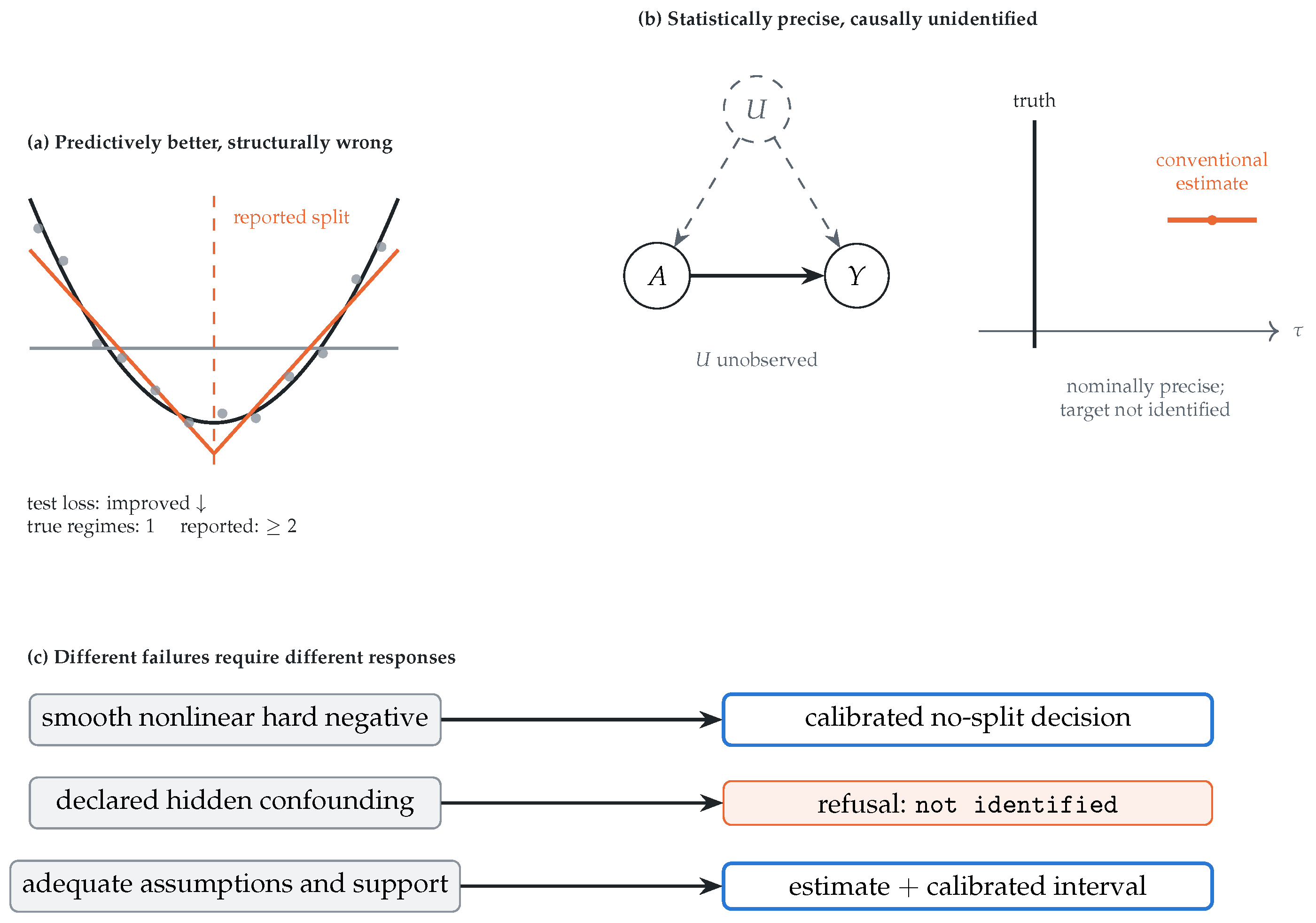
Figure 2.
Classical causal inference and amortized causal models as two incomplete halves. The classical side contributes identification theory, transparent estimators, and explicit assumptions, but requires manual method selection for every dataset; the amortized side contributes a reusable pretrained checkpoint, but typically operates inside an assumed causal setting without query-level refusal. CWFM inherits from both: the amortized component selects and orchestrates, while the estimators it orchestrates remain classical and are fitted anew to each submitted dataset.
Figure 2.
Classical causal inference and amortized causal models as two incomplete halves. The classical side contributes identification theory, transparent estimators, and explicit assumptions, but requires manual method selection for every dataset; the amortized side contributes a reusable pretrained checkpoint, but typically operates inside an assumed causal setting without query-level refusal. CWFM inherits from both: the amortized component selects and orchestrates, while the estimators it orchestrates remain classical and are fitted anew to each submitted dataset.
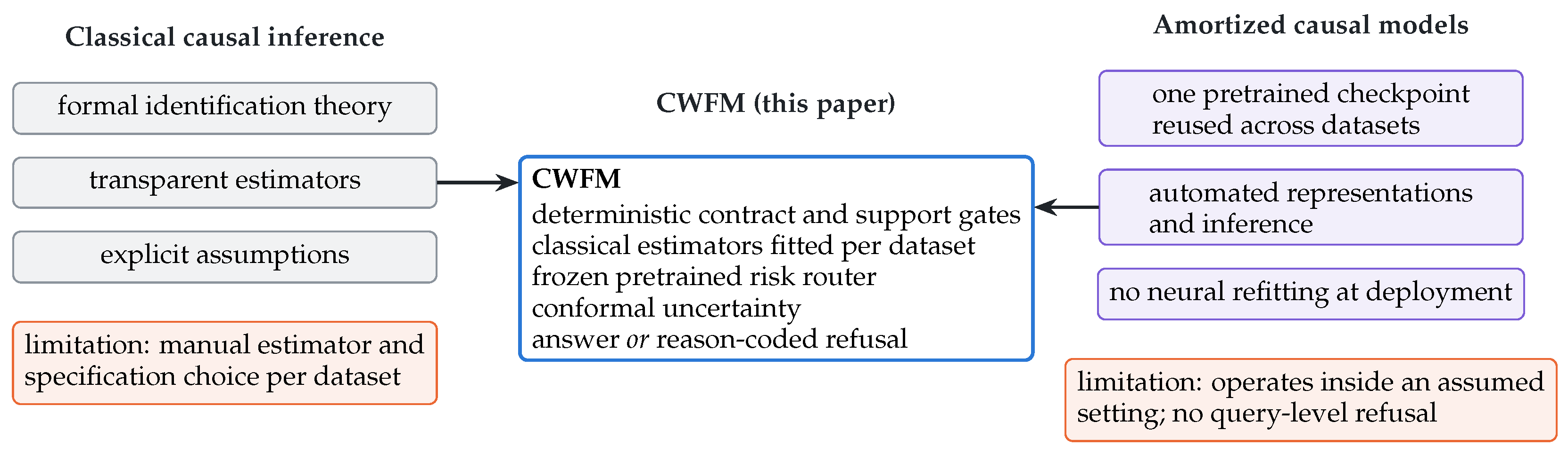
Figure 3.
The CWFM architecture in four lanes. The episode and the formal query merge into a declared causal contract, which three deterministic decisions check in sequence; each failure exits with a distinct structured status. For accepted queries, the classical estimator library is fitted to the submitted episode (gray) while the frozen encoder (violet) yields the representation from which the frozen risk router weights the compatible candidates into the compiled estimate (blue); the gated neural residual is effectively closed at the evaluated checkpoint (dashed). The output carries an estimate and interval only under the answer status, and learned diagnostics can warn but never override a gate.
Figure 3.
The CWFM architecture in four lanes. The episode and the formal query merge into a declared causal contract, which three deterministic decisions check in sequence; each failure exits with a distinct structured status. For accepted queries, the classical estimator library is fitted to the submitted episode (gray) while the frozen encoder (violet) yields the representation from which the frozen risk router weights the compatible candidates into the compiled estimate (blue); the gated neural residual is effectively closed at the evaluated checkpoint (dashed). The output carries an estimate and interval only under the answer status, and learned diagnostics can warn but never override a gate.
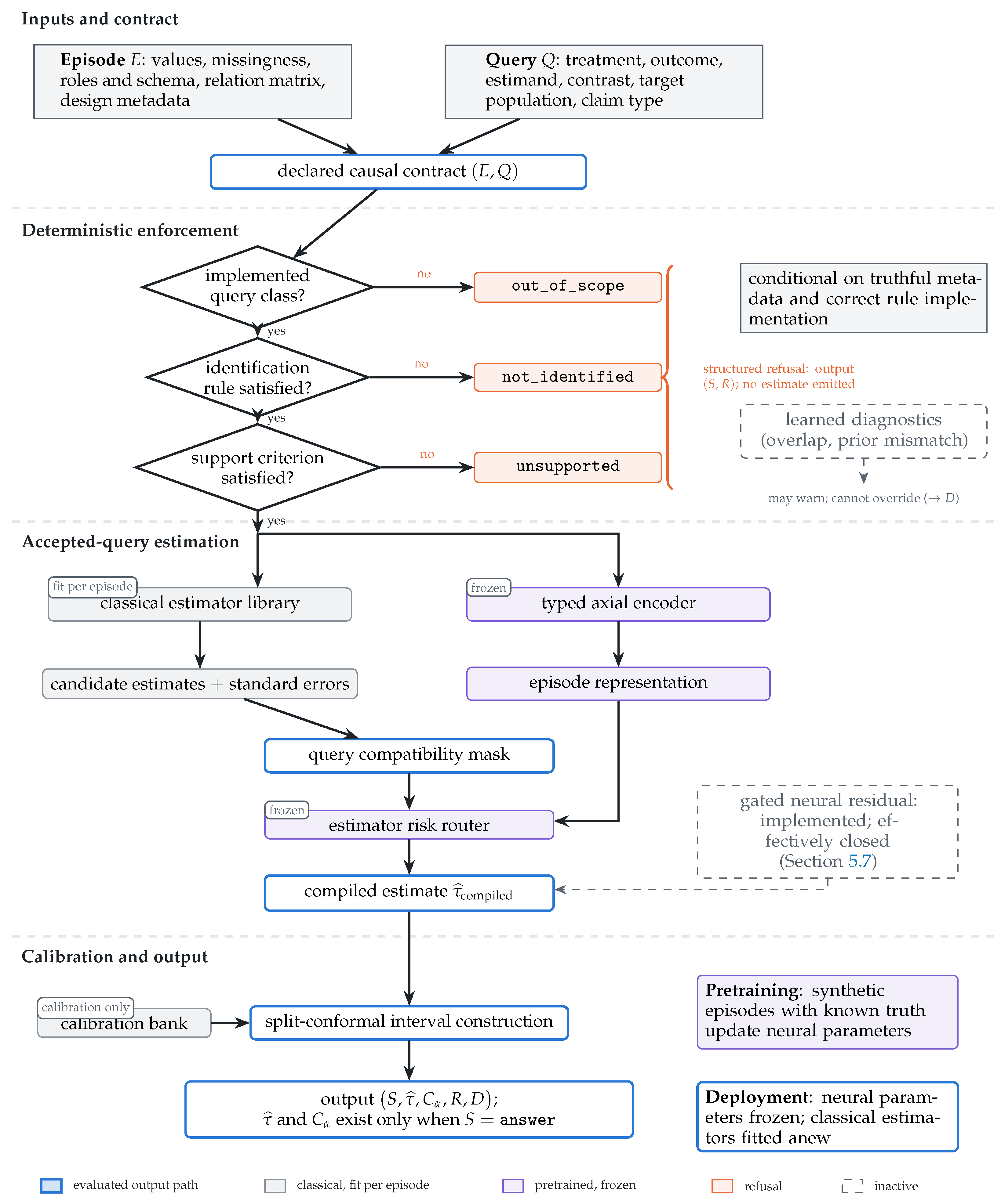
Figure 4.
Anatomy of the CWFM interface (schematic values). (a) A causal episode packages the observed table with declared roles, types, missingness (hatched cell), unit relations, and design metadata. (b) The formal query fixes the claim type, the estimand, and the requested contrast. (c) Query requirements, declared assumptions, and the implemented rule form the contract that the gates evaluate. (d) The output is one of four structured statuses; an estimate and interval exist only under answer; every refusal carries a machine-readable reason and a possible resolution.
Figure 4.
Anatomy of the CWFM interface (schematic values). (a) A causal episode packages the observed table with declared roles, types, missingness (hatched cell), unit relations, and design metadata. (b) The formal query fixes the claim type, the estimand, and the requested contrast. (c) Query requirements, declared assumptions, and the implemented rule form the contract that the gates evaluate. (d) The output is one of four structured statuses; an estimate and interval exist only under answer; every refusal carries a machine-readable reason and a possible resolution.
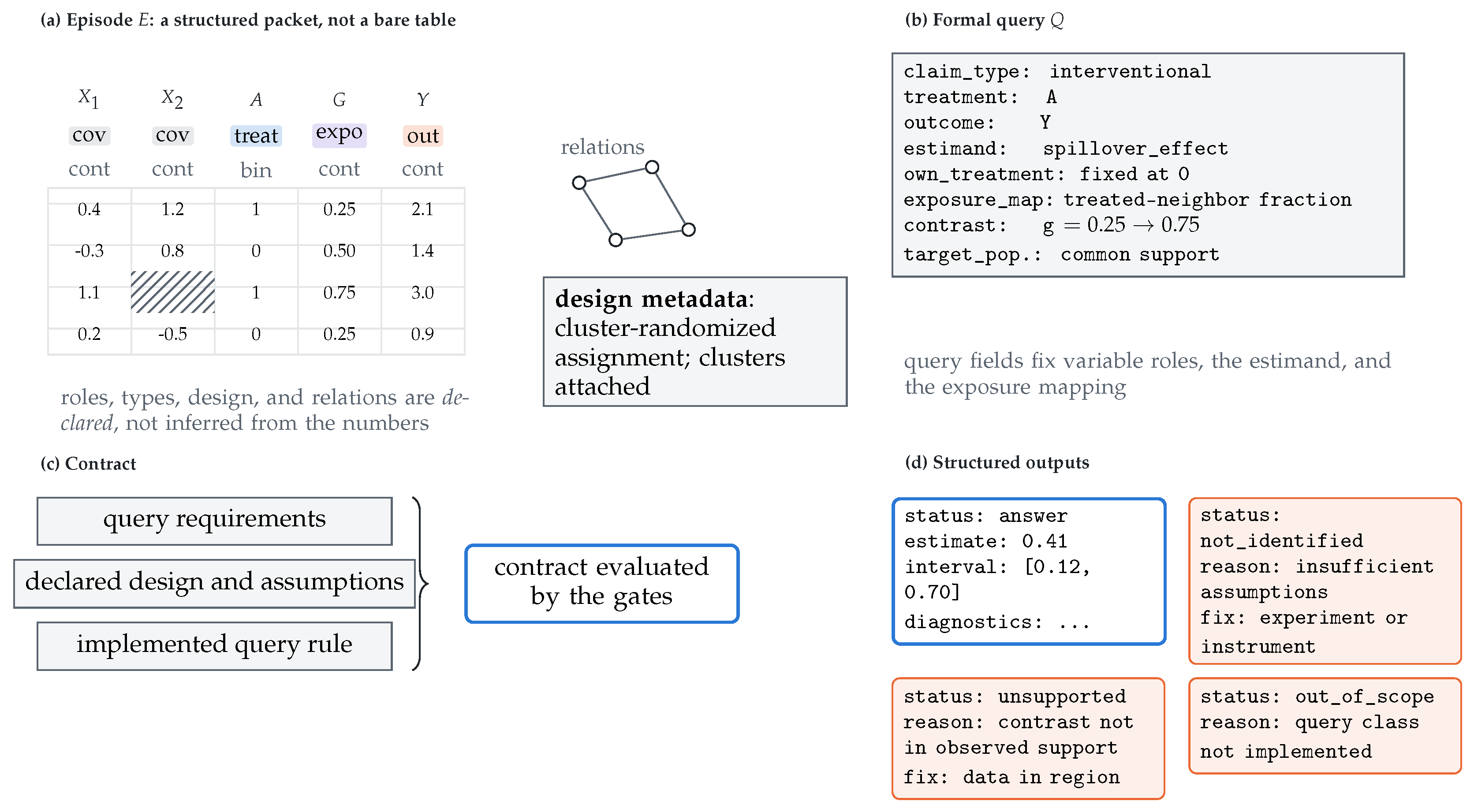
Figure 5.
Regime determination. (a) A smooth mechanism and a genuine threshold mechanism can fit equally well while differing structurally, so predictive gain alone never triggers a split. (b) Eligible covariates and candidate quantile thresholds span an evidence lattice; the maximum cell proposes the split variable and threshold. (c) The maximum evidence is compared against a threshold fitted on calibration episodes; this path produces the reported structure. (d) The hierarchical neural head is diagnostic at the evaluated checkpoint. (e) World particles are scored structural hypotheses whose weights remained effectively uniform in this run.
Figure 5.
Regime determination. (a) A smooth mechanism and a genuine threshold mechanism can fit equally well while differing structurally, so predictive gain alone never triggers a split. (b) Eligible covariates and candidate quantile thresholds span an evidence lattice; the maximum cell proposes the split variable and threshold. (c) The maximum evidence is compared against a threshold fitted on calibration episodes; this path produces the reported structure. (d) The hierarchical neural head is diagnostic at the evaluated checkpoint. (e) World particles are scored structural hypotheses whose weights remained effectively uniform in this run.
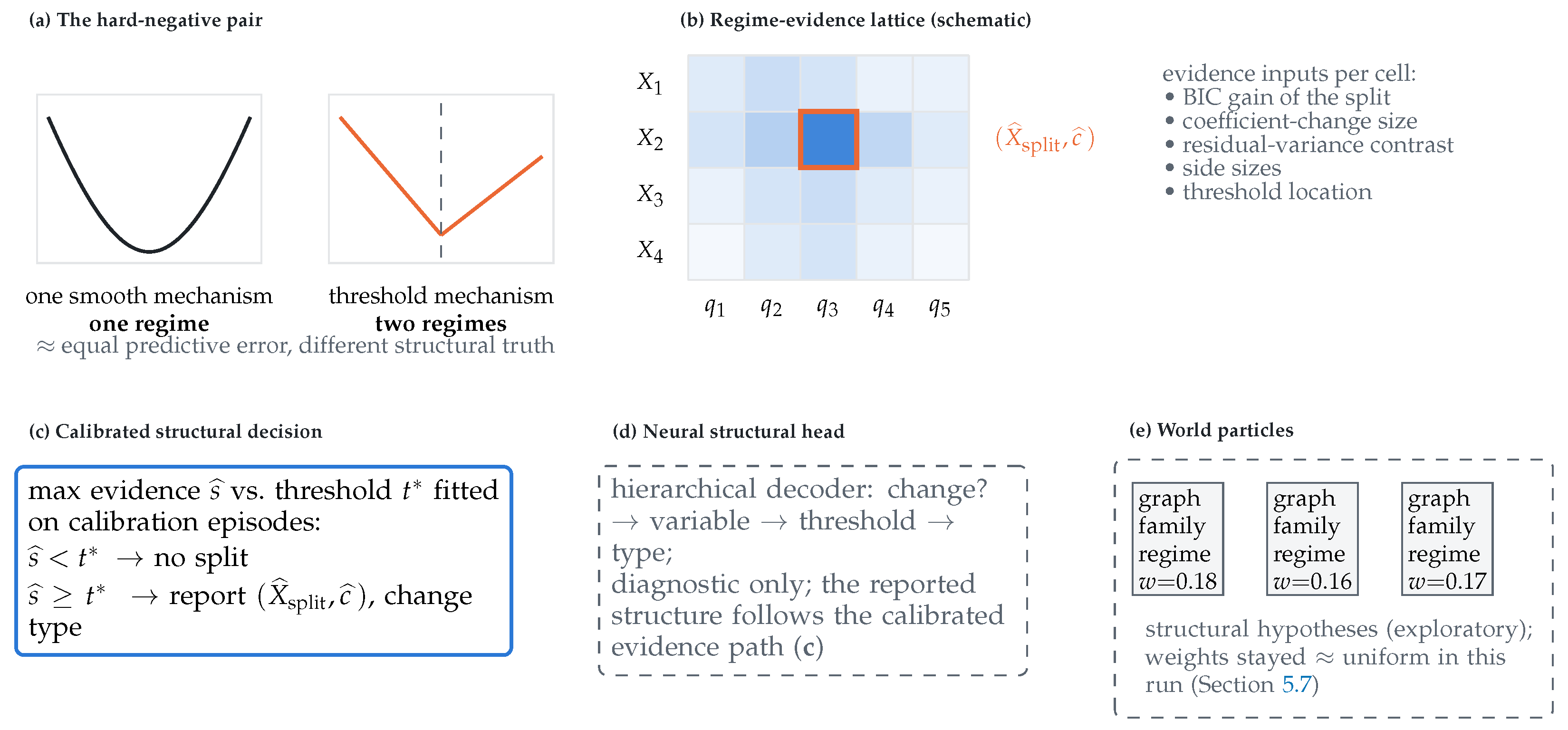
Figure 6.
Identification and support gates. Left: the decision sequence with its three refusal statuses; learned diagnostics sit outside the tree and can only warn. Right, top: the identification gate evaluates declared
knowledge; the same observed data are identified with a declared sufficient adjustment set and nonidentified without one. Right, bottom: the support gate evaluates the observed
sample; an exposure contrast with no observations near the requested level is refused as unsupported. The gates enforce the supplied contract; they do not establish that the supplied assumptions are true.
Figure 6.
Identification and support gates. Left: the decision sequence with its three refusal statuses; learned diagnostics sit outside the tree and can only warn. Right, top: the identification gate evaluates declared
knowledge; the same observed data are identified with a declared sufficient adjustment set and nonidentified without one. Right, bottom: the support gate evaluates the observed
sample; an exposure contrast with no observations near the requested level is refused as unsupported. The gates enforce the supplied contract; they do not establish that the supplied assumptions are true.
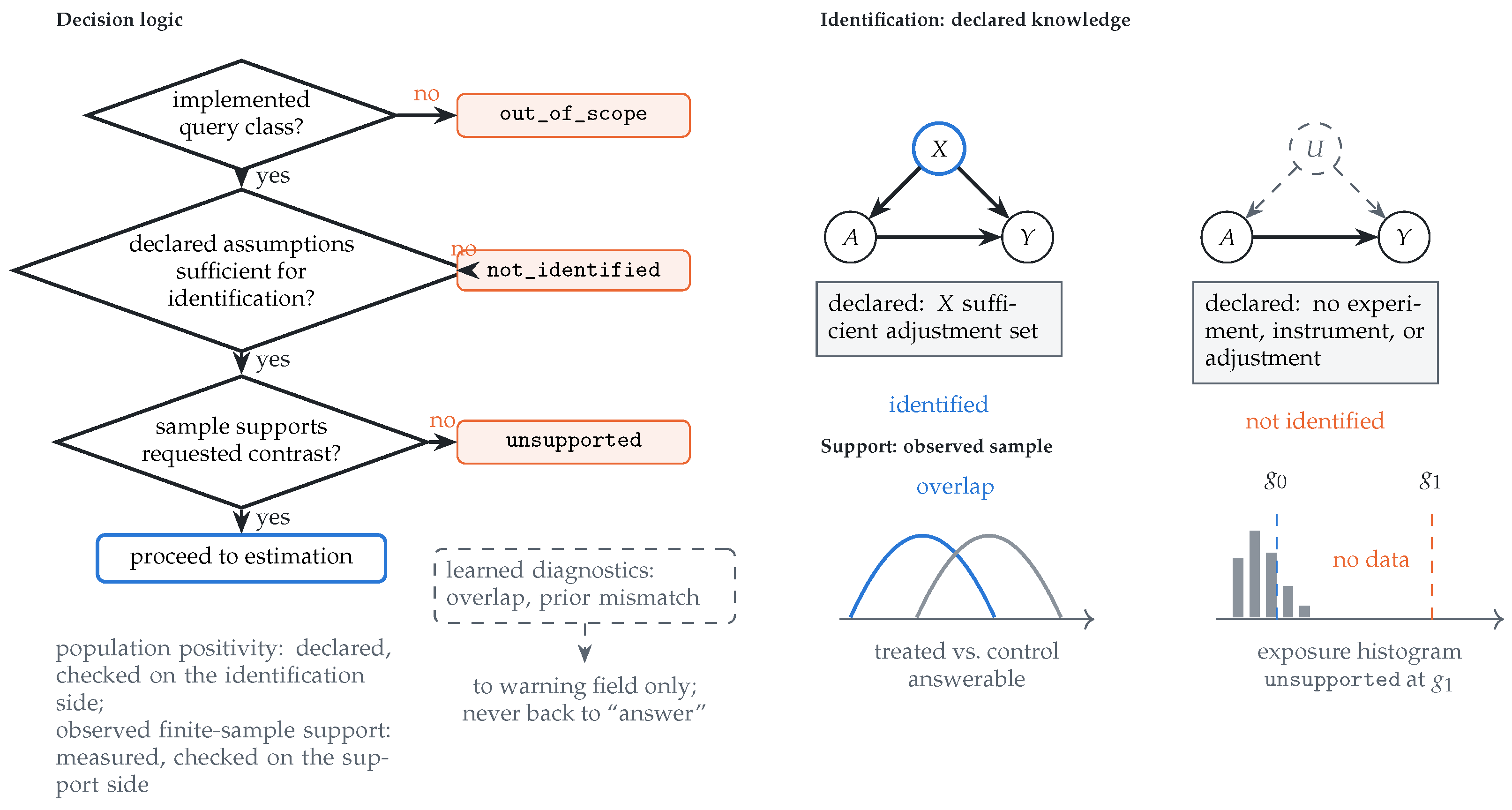
Figure 7.
From the estimator library to the final estimate (numbers schematic). Every query-compatible estimator is fitted to the submitted episode; the compatibility mask removes incompatible candidates, and the frozen router converts predicted relative risks into nonnegative weights that sum to one, yielding the compiled estimate. The gated neural residual could adjust it, but the correction must pass the no-harm gate, which is effectively closed at the evaluated checkpoint, so the final estimate equals the compiled one (Section 5.7).
Figure 7.
From the estimator library to the final estimate (numbers schematic). Every query-compatible estimator is fitted to the submitted episode; the compatibility mask removes incompatible candidates, and the frozen router converts predicted relative risks into nonnegative weights that sum to one, yielding the compiled estimate. The gated neural residual could adjust it, but the correction must pass the no-harm gate, which is effectively closed at the evaluated checkpoint, so the final estimate equals the compiled one (Section 5.7).
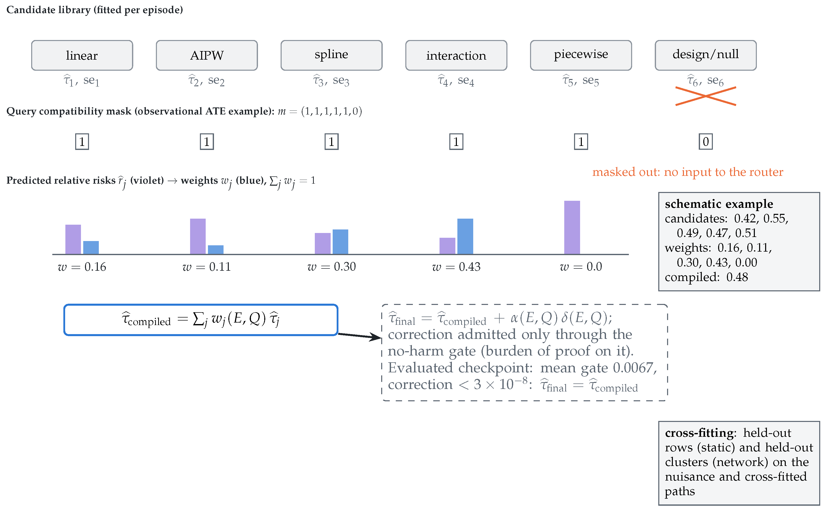
Figure 8.
Data generation and leakage prevention. Top: each episode starts from a fully sampled causal world; running it produces the material visible to CWFM, while the ground-truth labels stay behind a wall on the evaluator’s side. The declared design class is deliberately visible: it is the contract the gates enforce, not a label to recover. Bottom: the five streams draw from disjoint seed ranges; the out-of-distribution development lane is excluded from gradient training but informs checkpoint selection, and the locked test lane is evaluated exactly once after every upstream decision is frozen.
Figure 8.
Data generation and leakage prevention. Top: each episode starts from a fully sampled causal world; running it produces the material visible to CWFM, while the ground-truth labels stay behind a wall on the evaluator’s side. The declared design class is deliberately visible: it is the contract the gates enforce, not a label to recover. Bottom: the five streams draw from disjoint seed ranges; the out-of-distribution development lane is excluded from gradient training but informs checkpoint selection, and the locked test lane is evaluated exactly once after every upstream decision is frozen.
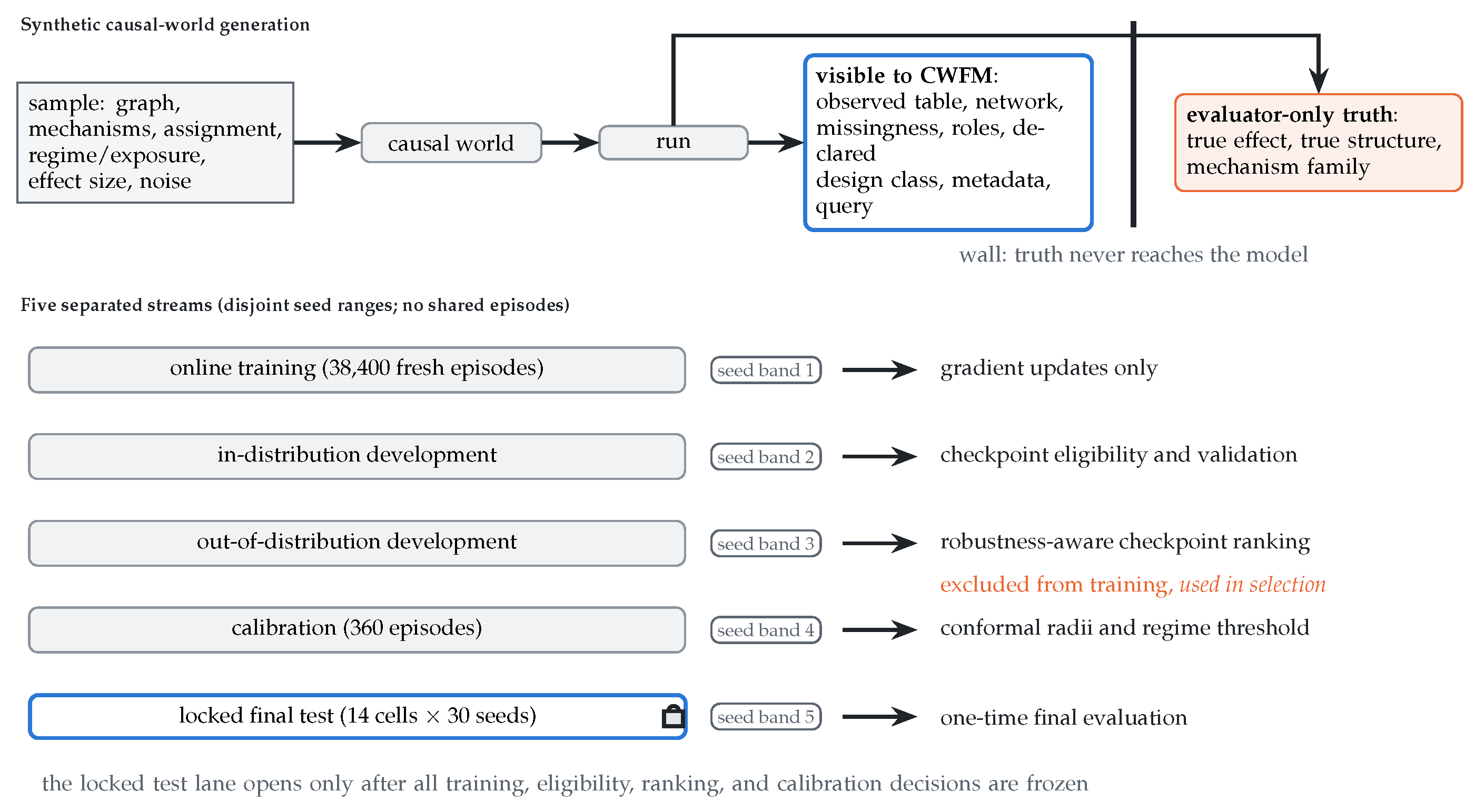
Figure 9.
Pooled results on the 180 answerable effect queries of the locked test bank. Left: mean absolute error of the estimated effect. Right: empirical coverage of the 90% intervals (dashed line: nominal target). CWFM (blue) matches the best always-answer specialists (gray) without knowing which mechanism generated each episode.
Figure 9.
Pooled results on the 180 answerable effect queries of the locked test bank. Left: mean absolute error of the estimated effect. Right: empirical coverage of the 90% intervals (dashed line: nominal target). CWFM (blue) matches the best always-answer specialists (gray) without knowing which mechanism generated each episode.
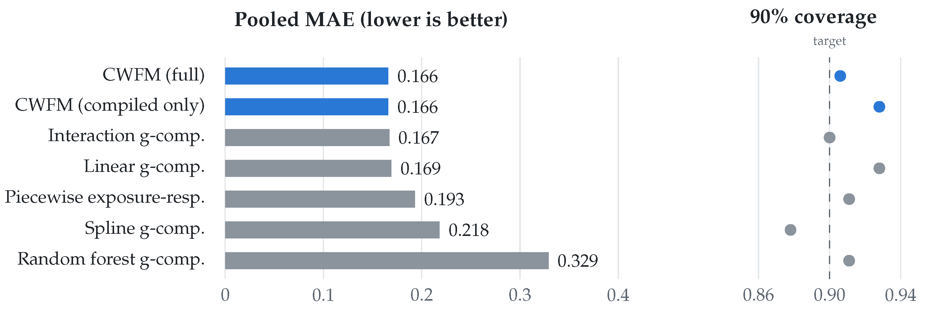
Figure 10.
Generalization to families excluded from gradient training (development diagnostic: four episodes per family, which also informed checkpoint selection). Most families (blue) stay near or moderately above the in-distribution error level (dashed line); nonmonotone interference (orange) degrades sharply, marking the limit of the synthetic training prior.
Figure 10.
Generalization to families excluded from gradient training (development diagnostic: four episodes per family, which also informed checkpoint selection). Most families (blue) stay near or moderately above the in-distribution error level (dashed line); nonmonotone interference (orange) degrades sharply, marking the limit of the synthetic training prior.
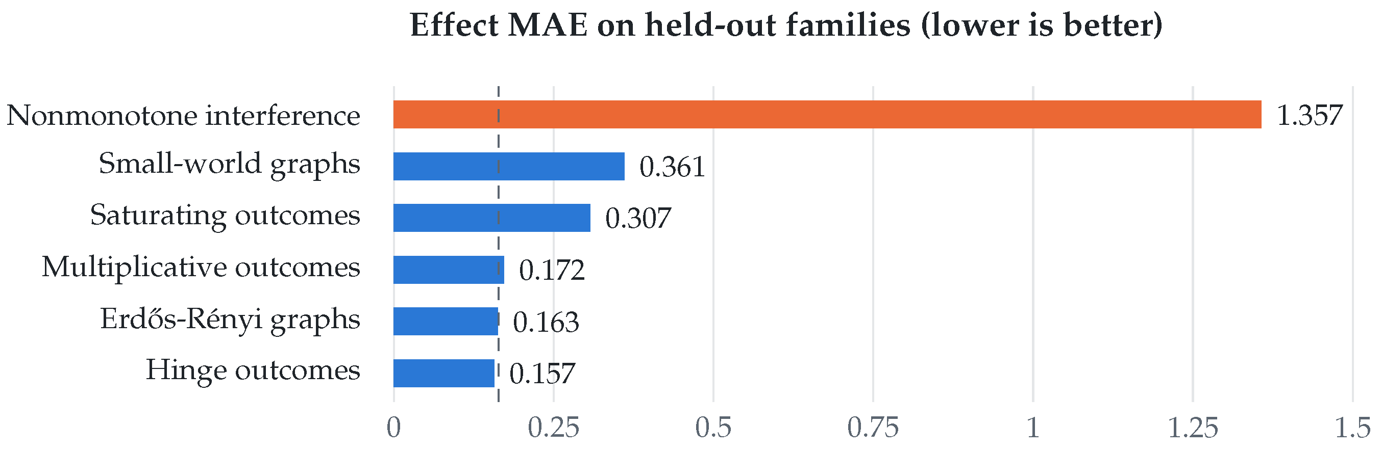
Figure 11.
The misspecification trap on one dataset. The true mechanism (dark line) is a single smooth quadratic with no regime change; a correctly specified quadratic local model (blue) reports no split, while a misspecified linear local model (orange) fits almost as well but only by inventing four regimes at the dashed boundaries. Predictive quality alone cannot distinguish the two conclusions.
Figure 11.
The misspecification trap on one dataset. The true mechanism (dark line) is a single smooth quadratic with no regime change; a correctly specified quadratic local model (blue) reports no split, while a misspecified linear local model (orange) fits almost as well but only by inventing four regimes at the dashed boundaries. Predictive quality alone cannot distinguish the two conclusions.
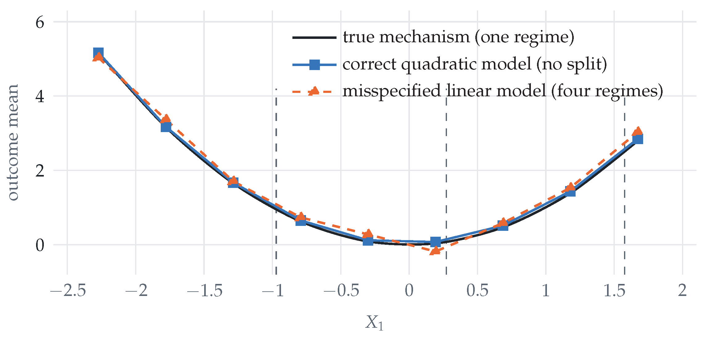

Table 1.
Interface positioning of representative systems. Cells describe the published interface; n/r (not reported) means the publication does not expose the capability as a first-class evaluated interface, not that it could not be added; n/a marks capabilities outside the system’s scope.
Table 1.
Interface positioning of representative systems. Cells describe the published interface; n/r (not reported) means the publication does not expose the capability as a first-class evaluated interface, not that it could not be added; n/a marks capabilities outside the system’s scope.
| System | Primary target | Identification handling | Support/ overlap handling | Estimator adaptation | Non-answer behavior |
|---|---|---|---|---|---|
| ID algorithm [10] | interventional distributions | complete graphical identification | n/a | n/a | proves nonidentifiability |
| DoWhy [11,12] | effect estimands | graphical, from user graph | diagnostics | user-selected library | refutation warnings |
| DECI [13] | graph and (C)ATE | learned graph, assumed class | n/r | single learned model | n/r |
| AutoCATE [35] | CATE | assumed ignorability | n/r | per-dataset selection, tuning, ensembling | n/r |
| Stacking / Q-aggregation [33,34] | (C)ATE | inherited from candidates | inherited | within-dataset aggregation | n/r |
| CausalFM [4] | effects in several settings | encoded in prior | n/r | amortized direct estimator | n/r |
| Do-PFN [5] | interventional outcomes | encoded in pretraining | n/r | amortized direct estimator | n/r |
| CausalPFN [21] | ATE and CATE | ignorability in prior | n/r | amortized direct estimator | n/r |
| ACTIVA [22] | post-intervention distributions | encoded in pretraining | n/r | amortized direct estimator | n/r |
| Causal conformal [44,46] | interval construction | inherited from base analysis | n/r | wraps any estimator | n/r |
| CWFM (this paper) | scalar effects, three query classes | finite rule library over declared contract | deterministic finite-sample gate | pretrained risk-routed blend of fitted classical estimators | typed statuses with machine-readable reasons |
Table 2.
Implemented query classes; the gates check the declared and support conditions before any listed estimator is fitted.
Table 2.
Implemented query classes; the gates check the declared and support conditions before any listed estimator is fitted.
| Query class | Declared conditions | Support condition | Estimators |
|---|---|---|---|
| Randomized ATE | Randomized treatment assignment | Both treatment arms present in the target population | Design-based; regression-adjusted |
| Observational ATE | Declared sufficient pre-treatment adjustment set | Treatment overlap over the target covariate region | Linear, interaction, and spline g-computation |
| Network spillover | Declared exposure mapping and assignment design | Support for the requested exposure contrast | Linear and piecewise exposure response |
Table 3.
The guarantee taxonomy of CWFM. Each row is a different kind of property; none implies the others.
Table 3.
The guarantee taxonomy of CWFM. Each row is a different kind of property; none implies the others.
| Property | What holds | Conditions | Not promised |
|---|---|---|---|
| Identification refusal | No estimate when the implemented rule evaluates to false | Correct rule implementation; truthful and sufficient declared metadata | That the declared assumptions are true; detection of undeclared confounding |
| Support refusal | Output suppressed when the support condition fails | Correct statistic, threshold, and implementation; in Section 5 the declared support class supplies the gate input | Population positivity; absence of all extrapolation; benchmarked behavior of the empirical statistic |
| Conformal interval | Episode-marginal coverage at the nominal level | Exchangeability with the calibration stream | Coverage per mechanism, for a fixed process, out of distribution, or on real data |
| No-harm residual | The correction met a non-degradation tolerance | The designated development banks and tolerance | Non-degradation on every episode |
| Zero false answers | No contract violation observed in the stress cells | The benchmark metadata and implemented gates | Recognition of undeclared or misdeclared violations |
| Out-of-prior reliability | Not established | Detection of or refusal on qualitatively new mechanisms |
Table 4.
MAE by scenario cell on the locked test bank (30 seeds per cell). Bold marks the best method per row. The combined column reports spline g-computation in the static rows and the piecewise exposure-response estimator in the network rows.
Table 4.
MAE by scenario cell on the locked test bank (30 seeds per cell). Bold marks the best method per row. The combined column reports spline g-computation in the static rows and the piecewise exposure-response estimator in the network rows.
| Scenario | CWFM | Linear | Interaction | Spline or piecewise | Rand. forest |
|---|---|---|---|---|---|
| Static linear | 0.168 | 0.160 | 0.189 | 0.181 | 0.412 |
| Static nonlinear | 0.190 | 0.218 | 0.163 | 0.169 | 0.502 |
| Static randomized | 0.150 | 0.141 | 0.154 | 0.145 | 0.449 |
| Network linear | 0.107 | 0.097 | 0.104 | 0.201 | 0.207 |
| Network threshold | 0.283 | 0.311 | 0.312 | 0.173 | 0.351 |
| Network null | 0.100 | 0.090 | 0.079 | 0.206 | 0.055 |
Table 5.
Principal causal targets of the compared foundation models, complementing the interface comparison of Table 1. ✓ marks a principal published evaluation target, ∼ a capability reported in some but not all published experiments; a blank cell means not a principal published target, not that it is impossible.
Table 5.
Principal causal targets of the compared foundation models, complementing the interface comparison of Table 1. ✓ marks a principal published evaluation target, ∼ a capability reported in some but not all published experiments; a blank cell means not a principal published target, not that it is impossible.
| Model | ATE | CATE/ITE | Do-query | Graph | Principal published evaluation |
|---|---|---|---|---|---|
| CWFM (this paper) | ✓ | Population causal-effect error | |||
| CausalPFN [21] | ✓ | ✓ | Treatment-effect error | ||
| Do-PFN [5] | ✓ | ∼ | ✓ | Interventional-query error | |
| CausalFM [4] | ∼ | ✓ | ∼ | CATE/ITE error (PEHE) | |
| Arrow [6] | ✓ | Structure and edge recovery | |||
| TabCausal [26] | ✓ | Structure and edge recovery | |||
| CDFM [7] | ✓ | Structure and edge recovery |
Table 6.
Regime determination on the locked test bank (30 seeds per cell). Structure accuracy requires selecting the correct split variable, or correctly selecting no split; threshold localization is not scored. Split rate is the fraction of episodes in which a regime split was declared.
Table 6.
Regime determination on the locked test bank (30 seeds per cell). Structure accuracy requires selecting the correct split variable, or correctly selecting no split; threshold localization is not scored. Split rate is the fraction of episodes in which a regime split was declared.
| CWFM | One-split baseline | |||
|---|---|---|---|---|
| Scenario | Structure | Split rate | Structure | Split rate |
| Strong split | 0.633 | 0.633 | 0.800 | 0.833 |
| Weak split | 0.000 | 0.000 | 0.033 | 0.033 |
| Stationary nonlinear (hard negative) | 0.833 | 0.167 | 0.000 | 1.000 |
| Complete null | 1.000 | 0.000 | 1.000 | 0.000 |
| Pooled structure accuracy | 0.617 | 0.458 | ||
Table 7.
Presentation-change probes at the evaluated checkpoint, each on a single static linear ATE episode: absolute change of the estimate under changes that should not matter.
Table 7.
Presentation-change probes at the evaluated checkpoint, each on a single static linear ATE episode: absolute change of the estimate under changes that should not matter.
| Probe | Absolute change in estimate |
|---|---|
| Row shuffling | |
| Rescaling the outcome by a positive factor | |
| Insertion of an irrelevant covariate | |
| Column reordering (roles preserved) |
Table 8.
Confirmatory test stream (1,800 fresh episodes, 300 per scenario; frozen checkpoint, no neural updates). MAE is pooled mean absolute error; the worst-cell column is the highest per-scenario MAE. Coverage is pooled empirical coverage under the shared 90% conformal protocol. The last column is the scenario-stratified paired bootstrap difference (router minus the row’s method) with its 95% interval; positive values favor the row’s method, and intervals excluding zero are bold. Oracles are non-deployable bounds.
Table 8.
Confirmatory test stream (1,800 fresh episodes, 300 per scenario; frozen checkpoint, no neural updates). MAE is pooled mean absolute error; the worst-cell column is the highest per-scenario MAE. Coverage is pooled empirical coverage under the shared 90% conformal protocol. The last column is the scenario-stratified paired bootstrap difference (router minus the row’s method) with its 95% interval; positive values favor the row’s method, and intervals excluding zero are bold. Oracles are non-deployable bounds.
| Method | MAE | Worst cell | Coverage | Router − method (95% CI) |
|---|---|---|---|---|
| Frozen-router soft blend | 0.161 | 0.286 | 0.886 | (reference) |
| Hard top-1 (frozen logits) | 0.163 | 0.308 | 0.886 | |
| Temperature-scaled router | 0.158 | 0.295 | 0.888 | |
| Uniform expert mean | 0.168 | 0.279 | 0.888 | |
| Median expert | 0.159 | 0.303 | 0.888 | |
| Best fixed expert | 0.163 | 0.307 | 0.879 | |
| Metadata-only selector | 0.162 | 0.307 | 0.882 | |
| Shallow risk selector | 0.141 | 0.191 | 0.888 | |
| Convex stack | 0.147 | 0.179 | 0.894 | |
| Oracle: per-cell expert | 0.117 | 0.166 | n/a | n/a |
| Oracle: per-episode expert | 0.067 | 0.092 | n/a | n/a |
Disclaimer/Publisher’s Note: The statements, opinions and data contained in all publications are solely those of the individual author(s) and contributor(s) and not of MDPI and/or the editor(s). MDPI and/or the editor(s) disclaim responsibility for any injury to people or property resulting from any ideas, methods, instructions or products referred to in the content. |
© 2026 by the author. Licensee MDPI, Basel, Switzerland. This article is an open access article distributed under the terms and conditions of the Creative Commons Attribution (CC BY) license.
Copyright: This open access article is published under a Creative Commons CC BY 4.0 license, which permit the free download, distribution, and reuse, provided that the author and preprint are cited in any reuse.