

Submitted:
04 August 2026
Posted:
05 August 2026
You are already at the latest version
Abstract
The usual power series \(\sum\alpha_{n}x^{n}\) are generalized by the substitution $x\to g(x)$ to power series built from a function \(\sum a_{n}g^{n}(x)\). The key feature of our approach consists in using functions \(g\) with free parameters \(g(x)=g(\{p_{i}\},x)\); the resulting expansions thus keep the Taylor‐like behavior (i.e., they match derivatives at the expansion point), but can also be tuned to adjust the far‐away behavior. We present six specific cases \(g_{X}\), $X\in\{A,\dots,F\}$, each containing five free parameters. We use examples to demonstrate that the generalization can improve the convergence (rate and domain), mimic branch points and branch cuts and have other interesting properties. Because the partial Bell polynomials are a necessary ingredient in our method, our results can be interpreted as new formulas for specific values of the Bell polynomials.
Keywords:
parametric approximations
; power expansions
; convergence rate
; convergence domain
1. Introduction
Many approximations can be seen as “matching” procedures [1]: interpolations match function values, (generalized) Fourier series and moment-problem solutions match weighted integrals and several expansions are based on matching derivatives. Besides the Taylor series, these include a number of other approximations (Padé approximants, Neumann series of Bessel functions, Lambert series, etc...). Thus, once the derivatives of a function at some point are known, one can choose the approximation from a finite set of existing possibilities. With each of them reproducing the function well in the neighborhood of the expansion point, we can select the one that describes the function best when the argument becomes larger. For example, it is well known that for some applications the Padé rational function provides a better description than the Taylor series.
We adopt a similar strategy: we construct derivative-matching approximations with tunable parameters, meaning that for each (well-defined, non-singular) parameter combination the resulting approximation matches derivatives at the expansion point. One can then use the parameters to tune the far-away behavior. We propose six formulas, with five free parameters each. In this way six infinite sets of adjustable approximations are built.
Alternatively, one can also interpret our results as new formulas for special values of the Bell polynomials, since these are necessary for our purposes.
2. Method
The method of construction is not new and proceeds through a substitution into the standard power series , as described in [2]. Reassessing our results there, we realized that some of them possess parametric freedom and this inspired us to investigate further. Adopting the notation
for an approximation , we assume, without loss of generality, that the expansion is performed at . Writing as
straightforward manipulations and Faà di Bruno’s formula give
where are (incomplete) Bell polynomials and . The existence of a non-vanishing derivative of g at zero guarantees the existence of the inverse function in some neighborhood of the same point.
Assuming we have a candidate function to be used in (1), the simplest way to find is to study higher-order derivatives of . Indeed, the latter can be understood as where and . Rewriting Faà di Bruno’s formula as
one uses to get
So, if one is able to derive an expression for in a way that does not rely on the Bell polynomials, i.e., then
Thus, finding a formula for the nth derivative of for some proposed g is one of the key concerns of this text. To implement parametric freedom, the free parameters are introduced into the definition of the function .
3. Properties
3.1. Existing Freedom
The Bell polynomials follow a transformation rule that reflects properties of differentiation
where q and w can be seen as parameters, which gives new possibilities for approximations. Indeed, if then
and
where . The latter expansion is trivial and does not represent a new approximation: the compensating scaling factor is introduced into the coefficients, but the summands remain identical. The former expansion is, however, non-trivial and we understand w as our first free parameter.
3.2. Convergence
Let I be the maximal open interval containing zero where g can be inverted. The question of convergence is then reduced to the convergence of the power series: the expansion converges for all such that , where is the radius of convergence of . To determine one uses standard power-series methods. In general, the convergence to the function is lost outside I. If two different arguments and give the same value then, obviously, the correct value is reconstructed for and the same value (which is generally incorrect) is obtained for , since the series cannot distinguish between and .
Although convergence properties can be straightforwardly related to power series, the approximation properties are non-elementary: the expansion of f may converge more rapidly and on a larger domain than the Taylor series of f. Consider a trivial example: with and the sum approximates f exactly and very rapidly: just one term suffices. The Taylor series converge only at and their convergence is slow (alternating sum). For , see the function from Definition 1 with , , , =1 and .
4. List
The following list of parametric functions consists of three pairs of inverse functions: any time a formula for was established then also an expression for was found: the roles of and can be swapped. It is unclear if this is just a coincidence or whether there is some deeper underlying reason. Parameters are included in the function names implicitly: . Also we define .
Definition 1.
The Python implementation of generalized expansions using these functions is submitted as supplementary material with this text.
Proposition 2.
Assume , and . Then , where are defined by (2) with
where
Formula (6) has a significant limit case without the quadratic term in the numerator
where , and tend to finite constants A, B and C. Thus
with , , , and one free parameter is lost. The corresponding limit of the formula for affects only the term:
Taking , one has
For the proofs, see the Appendix.
Proposition 3.
Assume , , and . Then , where are defined by (2) with
For proof see Appendix.
Remark 4.
The case gives correct results if approached as the limit .
Proposition 5.
Assume , , , and . Then , where are defined by (2) with
For the proof, see the Appendix.
Proposition 6.
Assume , , , , and . Then , where are defined by (2) with
where
For the proof, see the Appendix.
Remark 7.
The case gives correct results if approached as the limit .
Proposition 8.
Assume , , , and . Then , where are defined by (2) with
where
For the proof, see the Appendix.
Proposition 9.
Assume , , , , and . Then , where are defined by (2) with
where
and are the Stirling numbers of the first kind.
For the proof, see the Appendix.
Remark 10.
The case gives correct results if approached as the limit .
5. Case Studies
This chapter focuses on illustrative examples where proposed expansions are applied.
5.1. Increasing Convergence Rate and Domain of Power Series
In Section 3.2 we have demonstrated the convergence rate/domain enhancement using a somewhat degenerate (yet formally valid) case, in which the function being approximated was precisely the function used to build the series. Let us now provide a more “fair” example: we chose to approximate using with parameters , , , and , thus obtaining
which is bijective on . Besides elementary algebraic operations this formula uses only the square root which is evaluated very rapidly on a computer.
To investigate the behavior of the series
the inverse function is found to be
It gives
Using the standard expansion
and for all , one sees that the expressions for converge for all . One obtains
The summation no longer contains alternating signs, meaning that the expansion not only converges on the whole domain domain, but also converges more rapidly than the usual power expansion on . In addition, the convergence rate is enhanced by the absence of even powers.
In this studied example we used specific properties of the logarithm to find , which is, of course, also reproduced by the formula (17). The formula is, however, much more general and covers many additional cases in which an increase in the convergence rate or domain may be achieved, and which are more difficult to analyze.
5.2. Reproducing Branch Points
Let us approximate the Lambert W function by constructing an expansion for its principal branch at . We use , formulas (13) and (15), with parameters , and , where e is the base of the natural logarithm. Then
This choice creates a branch point for situated at , i.e., at the exact same position as the branch point between and . Doing this, one hopes to construct an expansion that works beyond the branch cut and where the branch is chosen by selecting the appropriate branch of the square root in (21), i. e. for .
Figure 1 shows the description of both branches by and . One observes that the second branch is approximated as well which can be justified rigorously. Indeed, one can understand the two W branches as situated on the branch cut which starts at and goes to . is then defined on its upper bank and on the lower bank. Thus, values are reached by transporting the values continuously around the branch point, not crossing the cut. It is known that the branch point is of the square-root type, so it can be removed by the substitution . Under this transformation, the upper bank remains unchanged (with a scaled argument), whereas the lower bank is “rotated” around and identified with . Consequently, the branch point is removed. Specifically, let us define
From preceding arguments it follows that the function is analytic at and the only (logarithmic) singularity of is situated at . By the transformation, it corresponds to the singularity of W on all Riemann sheets, excepted, at . What is the effect of the argument transformation on ? One has
We see that after the substitution the function used for the expansion becomes a simple linear function, , and the whole series becomes a derivative-matching power expansion , which is the Taylor series. This converges to the nearest singularity which, after removing the branching, is the logarithmic singularity at , see Figure 2. If converges to the unified branches , then, by back-substitution, converges to and , respectively. The back-substitution in fact gives a shifted Puiseux series.
Again, we have illustrated a feature of the approximations we propose on a simple example where the convergence can be easily demonstrated. Nevertheless, other parameter choices may also provide branch-point reconstruction (possibly with better convergence properties). For example, the numerical computations suggest that using with , , ,
one gets series that converge to W in the neighborhood of the branch point for both branches (see Figure 3), although this may be more difficult to prove.
5.3. Matching Value
Matching the function value at a point , different from the expansion point, is possible only in special situations.
5.3.1. Scenario with and
The generalized power series takes the value zero at whenever , a condition that can be realized by suitable parameter tuning. However, such an necessarily lies outside the interval I containing 0, on which g is bijective (recall that while ). Consequently, in any neighborhood of , the series will generally fail to converge to f. Nevertheless, this property remains useful, as it can still provide a rough approximation near specific points within the non-convergent region.
5.3.2. Scenario with and an Underlying Symmetry
In addition to , let us also assume:
- The symmetry ;
- The convergence for , where I is an interval containing zero on which g is bijective;
- The bound for all x, where J is the image of I, i.e., .
Proposition 11.
Under these strong conditions, we can conclude that
for all x.
Proof.
Indeed, for any , we have , so there exists such that . Since , the assumed convergence gives By the symmetry property, implies . Consequently, , and hence
Since was arbitrary, the desired convergence holds for all x. □
Let us show how this property can be useful using an example that we investigate only numerically. We chose and with parameters , , and , deliberately such that
i.e., the approximation reproduces the value of at . The symmetry of the functions with respect to
implies that if for then also for . The imposed constraint is expected to improve the approximation, for example when compared to the Taylor polynomial of the same degree. An objection can be made: because we add new information (about the symmetry), the improvement is not a surprise. This is only partially true. We may include the same information content also to an approximation based on a Taylor polynomial
thereby explicitly taking the symmetry into account. The results are shown in Figure 4. Clearly, the -based approximation outperforms significantly. This can be understood: besides the symmetry property, our approximation is analytic at for any partial approximation . We therefore believe that in a similar symmetry-backed situation the use of the value-matching procedure (value being zero) can be very useful and may considerably improve the convergence.
5.3.3. Optimizing Parameters
In previous paragraphs we have used specific parameters to demonstrate interesting features of new expansions without mentioning probably the most natural approach: tuning the parameters in an optimization procedure to best describe a function on a given interval. The aim would be to minimize the number of terms or the (computer) time to reach a desired precision. This ought to work: standard power expansions represent a single special case from the infinite set of parametric formulas we provide. There is no a priori reason why the global optimum should occur with the standard power series. Concerning computing time, they may win only if a small number of terms is taken into account, because our method requires computing from x. For a larger number of terms, one can expect the benefits of using (instead of x) to prevail. Let us also note that our expansions can be evaluated, like polynomials, by Horner’s method. Of course, for the generalized power series to be rapid, the coefficients need to be pre-computed, since they are computationally expensive. Thus a typical use case is to approximate a fixed function: compute the coefficients, store them, and use them repeatedly to evaluate the function for different arguments. We have made an effort to search for a mathematical function commonly implemented in numerical libraries (C, Java, Python, ...) for which our method could be competitive, at least on some reasonable interval. We did not succeed: the existing methods are fine-tuned over decades and use the power expansion (to be replaced by ours) very rarely; rather resorting to minimax polynomials and rational functions. Thus we believe our approach is more suited for specific, occasional situations where a solution to a problem is found as a non-standard (i.e., new, previously unknown) power series; it can then be enhanced.
Rather than providing a fully-tuned example let us focus on a specific optimization aspect: the parameter w is universal (present in all ) and computationally cheap. Tuning it may be a quick and routine way to improve the convergence. It does not appear deeply in formulas (12)-(20) and if these are used to compute for then , to be used with , see Section 3.1. It is therefore sufficient to remember a triangular array of numbers and search for an optimal w. The following example uses with , , and , i.e.,
The series with given by (20) is meant to approximate the Airy function Ai and we use the first six terms (). In the optimization, we start with the reference value and tune it so that the approximation reproduces the first zero of Ai, situated at . We find and present the results in Figure 5. We observe a very significant improvement and we see that the parameter tuning can hardly be compensated for by increasing the number of terms. We do not go beyond numerical observations in this example.
5.4. Manipulating Singularities
Assume f has a pole at and is analytic in its neighborhood for some . It may then seem natural to approximate it using a function g that also has a pole at the same position. Unfortunately this does not work well.
Proposition 12.
Let us define and assume that the set is infinite. Then there exists , , such that .
Proof.
By analyticity, we can write for and separate the regular part and the principal part . By definition is analytic (continuous) at , so there exists such that
This implies . The principal part has a finite number of terms, and consequently its value is dominated by once x becomes close to , i.e., there exists such that
Define and . Then, by the reverse triangle inequality
for all . Since g has a pole at and infinitely many coefficients are nonzero, the function has an essential singularity at . If does not converge for some , then the proof is complete. Otherwise, by Picard’s great theorem, takes all complex values in with at most one exception . Let and define
Since takes all values in infinitely many times in any neighborhood of , the set S is nonempty. For any we have
which implies . Thus does not converge to f on S. □
If f has an essential singularity in then the convergence is possible. There are simple examples, see e.g., Section 5.1 of [2].
Although poles cannot be directly approximated by the poles of g, one may use poles of g to improve the convergence rate. For example, define g with a shape (concavity/convexity, inflection point) similar to f. Let us give an example with . We use
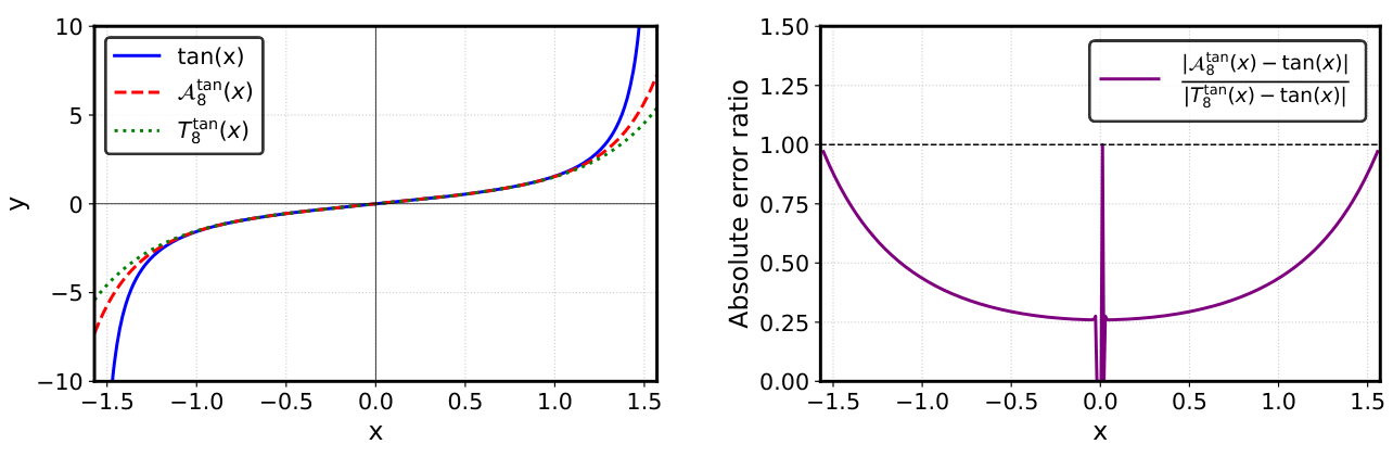
which corresponds to parameters , , , and with . Here i is the imaginary unit and are poles positions. One notices that is purely imaginary on the real axis and its imaginary part is odd and similar to , meaning it is increasing and antisymmetric with inflection point at the origin (Figure 6). By careful consideration of singularities of , the parameter is chosen so as to guarantee the convergence of the g power series on (see Section 3.2). By combining the odd powers of g (even ones are missing) with imaginary coefficients, a real-valued function is constructed. Numerical inspection (Figure 7) suggests that the approximation converges more rapidly than the Taylor series of the same length. One notices that the formula (24) is a very simple rational function that is fast to evaluate on a computer.
6. Discussion, Summary, Outlook
The expansions we present are derived from the simple idea of a substitution into a power series; we do not see additional sources for our work that should imperatively be cited. After conducting extensive literature and internet research, we firmly believe that the presented results are original, nevertheless, we acknowledge the existence of results with some degree of similarity, which deserve to be mentioned. Many of them have a higher mathematical complexity and are often targeted at specific physics problems.
A well-known method for improving convergence of a power series is the Euler transform [3]
where are computed as the nth order forward difference from coefficients . The method is well suited for summing alternating series and has generalization to negative indices [4] or to an approach dedicated to the summation of Rayleigh-Schrödinger series [5]. The formula (25) resembles what we present, but the factor reveals a difference.
Another mainstream approach for enhancing the convergence of series is Kummer’s transformation [6]. Aiming to speed up the convergence of , one searches for a similar series where C is known. Then S can be rewritten
with . If and behave alike as n increases, then tends to approach zero quickly.
A large number of publications stem from the seminal works of Aitken [7], Shanks [8] and Levin [9]. These authors introduced non-linear sequence transformations aimed at accelerating convergence by eliminating oscillations while preserving the underlying trend. Numerous other transformations have since been proposed [10,11,12], some of which incorporate free parameters. A nice overview is given in [13].
In fact, most of the methods mentioned above, as well as the method presented here, can be interpreted as conformal mappings, basically meaning substitution (or variable transformation), possibly with some terms re-arrangement. If done properly, it may move the point of evaluation from a position close to a singularity to a position far-away from the singularity, thus accelerating the convergence. Here, the essential texts to cite are by Van Dyke [14] and Guttmann [15].
An important approximation scheme is the Padé approximant which, by construction, is able to reproduce poles of the approximated function, thus possibly providing a good approximation even beyond this type of singularity. Here again, large generalizations exist: the authors of [16] propose a constructions where polynomials are replaced by general Chebyshev systems, thus possibly reproducing branch points and cuts. Another important application is the Padé-Borel summation, successfully implemented for example in quantum physics [17].
The latter citation is related to a topic many authors in physics and applied sciences work on: to give meaning to divergent series and to provide a mechanism for formally summing them up. Besides the Borel summation, one can mention order-dependent mapping methods [18], the variational perturbation theory [19] or more unconventional frameworks such as the self-similar approximation, a theory developed by Yukalov [20]. Nevertheless, these topics lie at the edge of the scope of this text.
We believe our construction surpasses previous approaches in several respects: the number and variety of both expansions and parameters, as well as their simplicity. The list of six functions we have presented is by no means exhaustive - one is free to invent his own g function, provided a formula for can be derived. The same applies to the number and meaning of the parameters; we have focused on five-parameter formulas only for convenience, and one may attempt to construct a g with an even larger number of adjustable parameters.
Apart from regularizing divergent series, our approximations can be used, as demonstrated, for all the other purposes mentioned above. Yet the construction remains remarkably simple. In principle, Bell polynomials can be expressed by a formula, but this formula is formal rather than explicit. It contains a summation symbol where the sum runs over all sequences of indices subject to specific constraints; this does not qualify as an explicit formulation in our view. In contrast, the formulas we provide are truly explicit: although lengthy, they rely solely on single summations with explicit summation limits. Furthermore, the convergence of our expansions is easily determined via back-substitution into power series. None of the competing approaches combines all these features.
We cannot foresee all possible applications of our construction, yet, given the sheer size of the field dedicated to enhancing power expansions, we believe our method can make a meaningful contribution. It remains for each researcher or scientist to adapt the tools we propose to their own needs. Our experience shows that parameter tuning is not always easy; in preparing the examples for this paper, we have explored many suboptimal parameter regions and encountered problematic local minima during optimization. Still, we have always succeeded in finding an expansion that met our requirements. We hope this will likewise be the case in future applications.
As a future prospect, we plan to establish a diverse library of parametric functions similar to to provide a broader range of options.
Very generally, extensions of existing mathematical definitions or constructions can be useful; in the past, we [21,22] and others [23,24,25] have contributed to the concept of differentiation by integration, which generalizes the ordinary derivative (extends the set of differentiable functions, provides algorithms to differentiate noisy data or can be used for fractional derivative) and is parameterized by an infinite (but not arbitrary) set of kernel functions. We believe this is also a path to follow in the future: one may investigate useful extensions of existing mathematical concepts, which, in relation to the present text, may for example consist in considering expansions to other approximation forms (not only powers-based) and principles (not only derivative-matching).
Data Availability Statement
No new data were created in this study. The research outputs consist of computer programs submitted as supplementary material with this text.
Use of Artificial Intelligence
The core ideas are the author’s own and can be traced back to a time before the widespread use of large language models [1,2]. However, AI tools (mostly DeepSeek [26] and Qwen [27]) were employed as supporting tools in the development of this text. Their role included providing assistance with the formulation of functions (6-), the derivation of equations (12-20), which were carefully checked by the author, and offering suggestions for the illustrative examples. Furthermore, the AI aided in proofreading and language refinement, while the initial drafting of the text was performed entirely by the author. It also assisted with the translation of the mathematical framework into the accompanying Python code. In all cases, the author has reviewed, validated, and taken full responsibility for the final output.
Acknowledgments
The author acknowledges the support of VEGA Grant No. 2/0084/25.
Appendix A. Proofs of Formulas ( uid11 )-( uid26 )
We have postponed the proofs of formulas (12)-(20) to appendix to make the text more readable. We work with expressions where the parameter w is missing, (meaning ) and we replace by x. Thanks to the formula (5) w is specific; it can be introduced later, once formulas with other parameters are established. As indicated in the text, formula (3), one needs to find the nth derivative of the kth power of the inverse function of g. First, let us list one useful formula
Appendix A.1. Lagrange-Bürmann Formula
Let f be an analytic function and let h be its inverse near . Then for any analytic function T
where denotes the coefficient of in the Taylor expansion of .
Appendix A.2. Proof of Formula ( uid11 )
Proof.
We assume and (and , ). The inverse function to , formula (6), is, in the neighborhood of , the function , formula (7), which can be verified by direct calculation. The latter is written as
One has
Introducing
one has
Let us work in the variable . We write where
This follows from the Lagrange-Bürmann formula with , :
We treat numerator and denominator in (A1) separately.
for any . The original condition (i.e., ) is taken care of automatically by the binomial coefficient . Next
which follows from the generalized binomial theorem for negative exponents. One extracts the coefficient in front of the term
If (i.e., ) then the last binomial coefficient is zero so we can restrict the summation limit over p to . Next, for the same binomial coefficient we use the identity , thus getting
Let us recall our aim: we seek a formula for . We have and . Thus
Using (4) we reproduce formula (12)
with given by (A2). Special limit cases (14) and (15) are derived by applying the limit to the previous procedure. □
Appendix A.3. Proof of Formula ( uid16 )
Proof.
We assume , and (, ). The inverse function to , formula (7), is, in the neighborhood of , the function , formula (6), which can be verified by direct calculation. The latter is written as
So
where the lower limit can be set to because gives a constant which disappears in the differentiation. Now we search for . Using the generalized binomial theorem we get
To extract the coefficient in front of we introduce a new index . Since one has
Analogically
With being a product of two terms, its factor can be expressed as a convolution
Substituting back to (A3) we get
This gives
which is identical to (16). □
Appendix A.4. Proof of Formula ( uid19 )
Proof.
We assume , , and (, ). The inverse function to , formula (8), is, in the neighborhood of , the function , formula (9), which can be verified by direct calculation. The latter is written as
We define , so and one has
Thus we search for . We define
We have . So, introducing , we have
The generalized binomial theorem gives
Next, let us focus on . We expand both parenthesis
Again, we express as convolution
Using we get
To complete the proof one needs to show that the upper summation index for p can be changed to n. If, for a fixed q, we define
then
i.e., the sum over q represents pth finite forward difference. At the same time the expressions and are, as function of q, polynomials of the order r and respectively. Thus their product has order n. Summing polynomials (index r) does not change the polynomial order. Therefore, if , the expression becomes zero since any finite difference operator with a degree higher than is the degree of the polynomial on which it acts gives zero. So . Then, using we get formula (17). □
Appendix A.5. Proof of Formula ( uid21 )
Proof.
We assume , , , and (, ). The inverse function to , formula (9), is, in the neighborhood of , the function , formula (8), which can be verified by direct calculation. The latter is written as
We start by defining
giving
Then
We remark that and we introduce : , where . We get
Then the generalized binomial theorem is used
With one expands . We are interested in the nth derivative at , i.e., in the nth coefficient of the power expansion. The expression implies that contributes at order , not earlier. We can safely truncate the series
Now we focus solely on the term.
so
Since , only terms contribute to the nth coefficient. One has
With obviously . This leads to
Now we put now everything together
After back-substitutions, using for , formula (18) is obtained
□
Appendix A.6. Proof of Formula ( uid24 )
Proof.
We assume , , and (, ). The inverse function to , formula (10), is, in the neighborhood of , the function , formula (11), which can be verified by direct calculation. The latter is written as
with
Then
Setting , we get
We focus on the last term
One has so . Therefore , when expanded, begins at or higher. Therefore
One has
The coefficient in front of is given by the convolution ()
This gives the final result
which is identical to (19). □
Appendix A.7. Proof of Formula ( uid26 )
Proof.
We assume , , , and (, ). The inverse function to , formula (11), is, in the neighborhood of , the function , formula (10), which can be verified by direct calculation. The latter is written as
We define
Then
So
Writing as with one has
Raising to the power gives
With , the power expansion of starts at or higher. We are interested in extracting the nth coefficient, so we write
This leads to
Again, the generalized binomial theorem is used for the last term
This can be related to the exponential generation function of the Stirling numbers of the first kind
We have
Taking into the account the relation between power-expansion coefficients and derivatives, one reproduces the formula (20)
where the innermost sum was truncated thanks to relations and for . □
References
- Liptaj, A. General Approach to Function Approximation. Mathematics 2024, 12. [Google Scholar] [CrossRef]
- Liptaj, A. Approximation by Power Series of Functions. Axioms 2025, 14. [Google Scholar] [CrossRef]
- Euler, L. Institutiones calculi differentialis cum eius usu in analysi finitorum ac doctrina serierum; Reprinted in Opera Omnia: Series 1, Volume 10; Academia Imperialis Scientiarum: Petropoli (St. Petersburg); Eneström Number E212, 1755; pp. 217–234. [Google Scholar]
- Borisov, B.; Shkodrov, V. Divergent series in the generalized binomial transform. Adv. Stud. Contemp. Math. 2007, 14, 77–82. [Google Scholar]
- Silverman, J.N. Generalized Euler transformation for summing strongly divergent Rayleigh-Schrödinger perturbation series: The Zeeman effect. Phys. Rev. A 1983, 28, 498(R)–501(R). [Google Scholar] [CrossRef]
- Kummer, E.E. Eine neue Methode, die numerischen Summen langsam convergirender Reihen zu berechnen. J. Für Die Reine Und Angew. Math. 1837, 1837, 206–214. [Google Scholar] [CrossRef]
- Aitken, A.C. On Bernoulli’s Numerical Solution of Algebraic Equations. Proc. R. Soc. Edinb. 1927, 46, 289–305. [Google Scholar] [CrossRef]
- Shanks, D. Non-linear Transformations of Divergent and Slowly Convergent Sequences. J. Math. Phys. 1955, 34, 1–42. Available online: https://onlinelibrary.wiley.com/doi/pdf/10.1002/sapm19553411. [CrossRef]
- Levin, D. Development of non-linear transformations for improving convergence of sequences. Int. J. Comput. Math. 1972, 3, 371–388. [Google Scholar] [CrossRef]
- Wynn, P. On a Device for Computing the em(Sn) Transformation. Math. Tables Other Aids To Comput. 1956, 10, 91–96. [Google Scholar] [CrossRef]
- Čížek, J.; Zamastil, J.; Skála, L. New summation technique for rapidly divergent perturbation series. Hydrogen atom in magnetic field. J. Math. Phys. 2003, 44, 962–968. Available online: https://pubs.aip.org/aip/jmp/article-pdf/44/3/962/19259570/962_1_online.pdf. [CrossRef]
- Woźny, P.; Nowak, R. Method of summation of some slowly convergent series. Appl. Math. Comput.;Phys. Comput. 2009, 215, 1622–1645. [Google Scholar] [CrossRef]
- Weniger, E.J. Nonlinear sequence transformations for the acceleration of convergence and the summation of divergent series. Comput. Phys. Rep. 1989, 10, 189–371. [Google Scholar] [CrossRef]
- VAN DYKE, M. ANALYSIS AND IMPROVEMENT OF PERTURBATION SERIES. Q. J. Mech. Appl. Math. 1974, 27, 423–450. Available online: https://academic.oup.com/qjmam/article-pdf/27/4/423/5234513/27-4-423.pdf. [CrossRef]
- Guttmann, A.J. Asymptotic Analysis of Power-Series Expansions. In Phase Transitions and Critical Phenomena; Domb, C., Lebowitz, J.L., Eds.; Academic Press: San Diego, 1989; Vol. 13, pp. 1–128. [Google Scholar]
- Barnsley, M.F.; Bessis, D. Padé approximant bounds on the positive solutions of some nonlinear elliptic equations. Proc. R. Soc. Edinb. Sect. A Math. 1978, 80, 183–200. [Google Scholar]
- Graffi, S.; Grecchi, V.; Simon, B. Borel summability: Application to the anharmonic oscillator. Phys. Lett. B 1970, 32, 631–634. [Google Scholar] [CrossRef]
- Seznec, R.; Zinn-Justin, J. Summation of divergent series by order dependent mappings: Application to the anharmonic oscillator and critical exponents in field theory. J. Math. Phys. 1979, 20, 1398–1408. Available online: https://pubs.aip.org/aip/jmp/article-pdf/20/7/1398/19145091/1398_1_online.pdf. [CrossRef]
- Kleinert, H.; Janke, W. Convergence behavior of variational perturbation expansion — A method for locating Bender-Wu singularities. Phys. Lett. A 1995, 206, 283–289. [Google Scholar] [CrossRef]
- Yukalov, V.I.; Yukalova, E.P. From Asymptotic Series to Self-Similar Approximants. Physics 2021, 3, 829–878. [Google Scholar] [CrossRef]
- Liptaj, A. Maximal generalization of Lanczos’ derivative using one-dimensional integrals. Palest. J. Math. 2021, 10, 694–699. [Google Scholar]
- Liptaj, A. Higher accuracy order in differentiation-by-integration. Math. Model. Anal. 2021, 26, 304–317. [Google Scholar] [CrossRef]
- Diekema, E.; Koornwinder, T.H. Differentiation by integration using orthogonal polynomials, a survey. J. Approx. Theory 2012, 164, 637–667. [Google Scholar] [CrossRef]
- Cruz-Santiago, R.; López-Bonilla, J.; López-Vázquez, R. Differentiation of Fourier Series via Orthogonal Derivative. J. Inst. Sci. Technol. 2015, 20, 113–114. [Google Scholar] [CrossRef]
- Teruel, G.R.P. Kernel-based integral derivative operators with applications to quantum systems. J. Phys. A Math. Theor. 2026, 59, 275201. [Google Scholar] [CrossRef]
- DeepSeek-AI. Deep. Large Lang. Model (Web interface) Accessed. 2026. (accessed on 2026-07-23).
- Alibaba Group. Qwen Large Language Model (Web interface). Accessed. 2026. (accessed on 2026-07-23). [Google Scholar] [CrossRef]
Figure 1.
Description of both branches of the Lambert W function by -series with different branches of the square root, see formula (21).
Figure 1.
Description of both branches of the Lambert W function by -series with different branches of the square root, see formula (21).
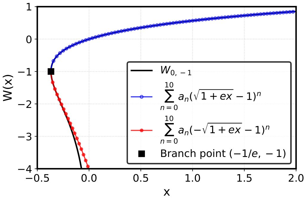
Figure 2.
Branches become one analytic function at with the branch point removed. Sum represents its Taylor series expanded at .
Figure 2.
Branches become one analytic function at with the branch point removed. Sum represents its Taylor series expanded at .
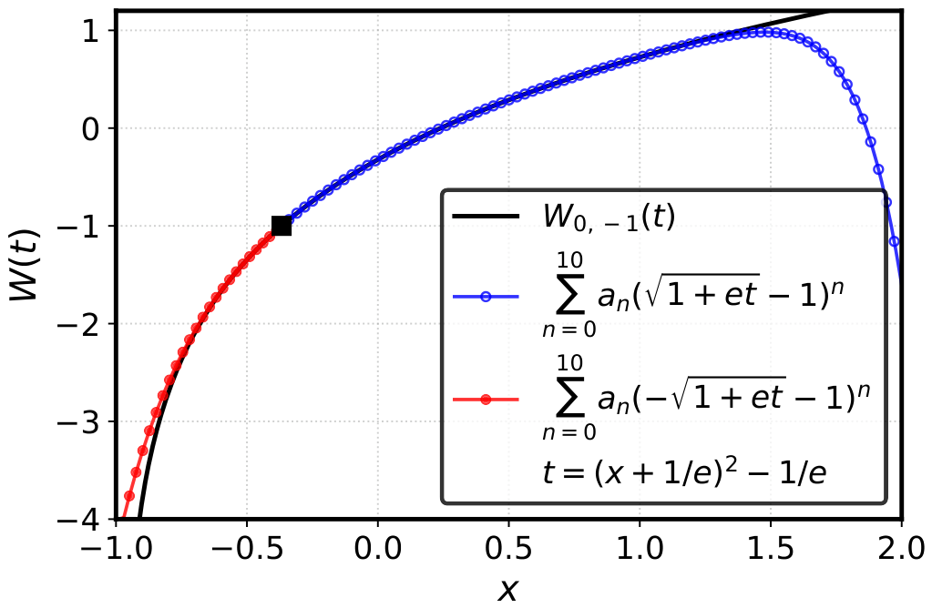
Figure 3.
Branches approximated using the expansion with from (22).
Figure 3.
Branches approximated using the expansion with from (22).
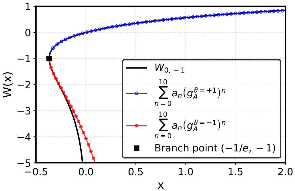
Figure 4.
The approximation of by and by symmetrized Taylor polynomial , formula (23), on the left, and the corresponding errors on the right.
Figure 4.
The approximation of by and by symmetrized Taylor polynomial , formula (23), on the left, and the corresponding errors on the right.
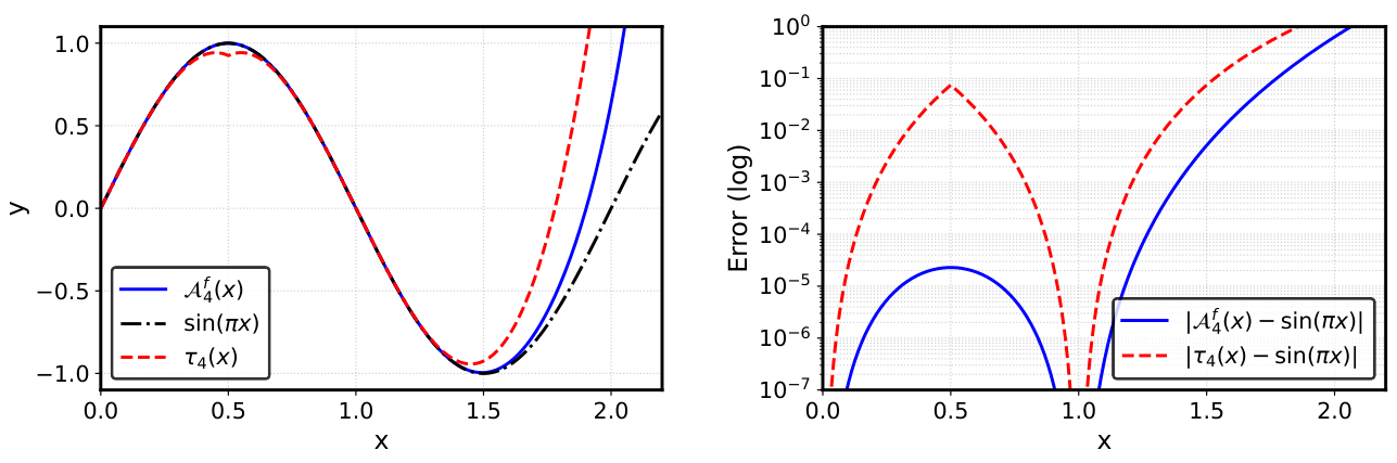
Figure 5.
For the approximation of Ai using , tuning w to reproduce the zero at improves the accuracy much more than increasing N.
Figure 5.
For the approximation of Ai using , tuning w to reproduce the zero at improves the accuracy much more than increasing N.
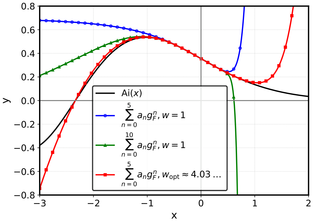
Figure 6.
The imaginary and real part of , formula (24). From the perspective of the origin, the poles are situated (quite) beyond those of , latter denoted by dotted lines.
Figure 6.
The imaginary and real part of , formula (24). From the perspective of the origin, the poles are situated (quite) beyond those of , latter denoted by dotted lines.
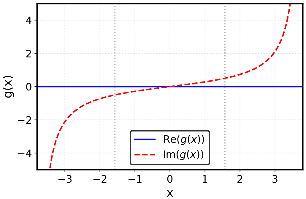
Figure 7.
Left picture: Approximation of by and by the Taylor series . Right picture: Comparison of errors by ratio.
Figure 7.
Left picture: Approximation of by and by the Taylor series . Right picture: Comparison of errors by ratio.
Disclaimer/Publisher’s Note: The statements, opinions and data contained in all publications are solely those of the individual author(s) and contributor(s) and not of MDPI and/or the editor(s). MDPI and/or the editor(s) disclaim responsibility for any injury to people or property resulting from any ideas, methods, instructions or products referred to in the content. |
© 2026 by the authors. Licensee MDPI, Basel, Switzerland. This article is an open access article distributed under the terms and conditions of the Creative Commons Attribution (CC BY) license (http://creativecommons.org/licenses/by/4.0/).
Copyright: This open access article is published under a Creative Commons CC BY 4.0 license, which permit the free download, distribution, and reuse, provided that the author and preprint are cited in any reuse.