Preprint
Article

This version is not peer-reviewed.

Physics-Informed Transfer Learning Reduces Simulation to Reality Gaps for Winter Wheat Traits Retrieval from Hyperspectral Observations

Submitted:

03 August 2026

Posted:

05 August 2026

You are already at the latest version

Abstract

Accurate retrieval of crop structural and physiological traits from remote sensing data remains challenging due to limited field observations and poor cross-platform generalization of data-driven models. This study develops a physics-informed transfer learning framework to quantify the contributions of improving simulated data fidelity and increasing model complexity to retrieving winter wheat leaf area index (LAI) and canopy chlorophyll content (CCC) from hyperspectral observations. Two PROSAIL-D datasets with default and physically optimized leaf angle distributions were generated to represent different levels of simulation fidelity. Four dual-branch deep learning architectures (CNN, CNN–SE, CNN–Transformer, and CNN–SE–Transformer) integrating spectral bands and vegetation indices were pretrained on simulated datasets and transferred to real observations using progressive fine-tuning. Model performance was assessed using ground-based and unmanned aerial vehicle (UAV) hyperspectral datasets, and SHapley Additive exPlanations (SHAP) analysis was applied to interpret feature contributions. Results demonstrated that transfer learning substantially improved cross-domain generalization, while enhancing simulation fidelity provided greater performance gains than increasing network complexity. The CNN–Transformer model pretrained on physically optimized simulations achieved the highest accuracy and robustness for both LAI and CCC retrieval. At ground and UAV scales, it achieved LAI estimation accuracies of R2 = 0.55 (RMSE = 0.63) and R2 = 0.53 (RMSE = 0.62), respectively. For CCC estimation, the model obtained R2 = 0.59 at both scales, with RMSE values of 36.12 μg cm⁻2 and 37.56 μg cm⁻2 for ground and UAV observations, respectively. SHAP analysis indicated that physically optimized simulations shifted model attention toward physiologically relevant vegetation indices, whereas default simulations induced stronger dependence on unstable visible wavelengths. Physically informed simulation design combined with transfer learning effectively reduces simulation to reality discrepancies, whereas increasing deep model complexity alone provides limited improvement. The proposed framework offers an accurate, interpretable, and scalable solution for cross-platform crop trait retrieval from hyperspectral observations.
Keywords: 
;  ;  ;  ;  ;  

1. Introduction

Winter wheat is a globally significant staple crop and plays a pivotal role in ensuring food security and sustaining agricultural production systems worldwide [1,2]. Reliable and timely monitoring of its growth status is therefore critical for optimizing field management practices, enhancing nitrogen use efficiency, and improving yield forecasting under increasing climatic variability [3,4,5]. Among key biophysical variables, leaf area index (LAI) and canopy chlorophyll content (CCC) constitute fundamental descriptors of crop canopy structure and physiological function, respectively. LAI quantifies vegetation density and light interception capacity [6,7], whereas CCC serves as an indicator of photosynthetic potential and nitrogen status [8,9]. Their complementary nature enables a more comprehensive characterization of crop growth dynamics than single-variable analyses [10].
Hyperspectral remote sensing has emerged as an effective non-destructive approach for retrieving crop biophysical parameters owing to its rich spectral information content [11,12]. Conventional retrieval methods primarily rely on vegetation indices (VIs), which utilize predefined spectral band combinations to infer crop traits. Despite their computational efficiency and widespread adoption, these indices exhibit notable limitations, including site dependency, sensitivity to soil background effects, and spectral saturation under high canopy density conditions [13,14]. These constraints substantially impair their transferability across environments and phenological stages. To overcome these limitations, physically based radiative transfer models (RTMs), such as PROSAIL, have been introduced for crop parameter retrieval. RTM-based approaches offer strong physical interpretability and improved generalization capacity. However, their practical application is hindered by two fundamental challenges: high computational cost and the ill-posed nature of the inverse problem, whereby multiple parameter combinations may yield similar spectral responses [13,15].
To address the high dimensionality and nonlinear characteristics of hyperspectral data, machine learning methods such as random forest (RF), support vector regression (SVR), and Gaussian process regression (GPR) have been widely employed [16,17,18]. Nevertheless, these approaches depend heavily on handcrafted features, which inevitably discard subtle yet informative spectral structures, thereby constraining generalization under complex canopy conditions [19,20]. With advances in artificial intelligence, deep learning (DL) has become the dominant paradigm for remote sensing inversion due to its strong capability for automatic feature representation learning [21,22]. Convolutional neural networks (CNNs) extract hierarchical spectral features directly from raw hyperspectral inputs, reducing reliance on manual feature engineering [23]. Subsequent developments introduced recurrent neural networks (RNNs) and long short-term memory (LSTM) models to capture sequential spectral dependencies. More recently, attention mechanisms and transformer-based architectures have further enhanced the modeling of long-range spectral dependencies, particularly in physically informative regions such as red-edge and near-infrared bands [24]. Despite these advances, several limitations persist. CNN-based models primarily capture local spectral patterns but exhibit limited capability in modeling global spectral dependencies. RNN-based architectures suffer from restricted parallelization and vanishing gradient issues when processing long sequences [25]. Although transformer models partially alleviate these constraints, their effectiveness is strongly dependent on large-scale labeled datasets [26].
A critical bottleneck in agricultural remote sensing is the scarcity of high-quality labeled field data. Unlike computer vision domains, the acquisition of LAI and CCC measurements requires destructive sampling and labor-intensive biochemical analysis. Consequently, available datasets are typically limited in size, spatial coverage, and temporal continuity. This data scarcity often leads to severe overfitting when training deep models on field observations alone, thereby reducing cross-domain generalization performance. To mitigate this limitation, transfer learning (TL) has been widely adopted in crop trait retrieval. In particular, simulation to reality transfer learning based on radiative transfer models (RTMs) has emerged as a dominant paradigm. Within this framework, large-scale simulated spectral datasets are generated under controlled physical assumptions to pretrain deep networks, enabling them to learn generalized radiative transfer relationships, which are subsequently adapted to real-world observations through fine-tuning [22,27].
Recent studies have demonstrated that transfer learning, combined with improved feature engineering or advanced architectures, can enhance crop trait retrieval under limited data conditions [28,29]. However, most existing approaches primarily focus on algorithmic improvements and treat RTM-generated data as a fixed and reliable supervisory source. Within this paradigm, performance gains are largely attributed to increased model complexity, architectural refinement, or feature fusion strategies. This perspective neglects a more fundamental issue: the physical fidelity of simulated data may deviate from real canopy structures due to simplified or imperfectly parameterized RTM assumptions. Consequently, even highly complex models cannot fully compensate for systematic biases embedded in simulated data generation. In such cases, increasing model complexity may yield diminishing returns while incurring additional computational cost. To address this gap, this study investigates the relative roles of physical prior fidelity and model complexity in simulation to reality crop trait retrieval. Specifically, three research questions are posed: (i) whether improving the physical fidelity of RTM-generated simulations enhances LAI and CCC retrieval performance more effectively than increasing model complexity; (ii) how physically optimized simulation parameters influence feature representation and decision mechanisms under cross-scale transfer scenarios; and (iii) whether transfer learning can effectively mitigate simulation to reality discrepancies under imperfect physical priors.
In this study, a hybrid deep learning framework integrating CNN and transformer encoders is developed to jointly capture local spectral features and global spectral dependencies from hyperspectral observations. To examine the role of physical prior quality, two PROSAIL-D simulation datasets are constructed using default settings (Dataset I) and physically optimized leaf angle distribution parameters (Dataset II) derived from field measurements, respectively. Based on these datasets, four representative network architectures with increasing complexity are systematically evaluated under two training strategies: direct simulation training (without TL) and simulation to reality transfer learning with fine-tuning (with TL). The model’s performance was evaluated against multi-scale datasets comprising ground-based hyperspectral measurements and unmanned aerial vehicle (UAV) hyperspectral imagery captured over winter wheat. Finally, SHapley Additive exPlanations (SHAP) are employed to interpret model predictions and quantify how physical prior optimization and transfer learning affect feature attribution patterns across spectral regions.

2. Materials and Methods

2.1. Study Area and Field Experiments

This study utilized ground-based winter wheat datasets collected in Beijing, China, during 2002, 2004, 2019 and 2021 to evaluate the performance of the proposed retrieval framework. Field experiments were conducted at the National Precision Agriculture Research Station in Xiaotangshan, Changping District, Beijing (40°10′48″N, 116°26′24″E). The study area is characterized by a warm temperate, semi-humid monsoon climate, with a mean annual temperature of approximately 13 °C and mean annual precipitation of approximately 508 mm, the majority of which occurs between June and August, coinciding with the crop growing season. To ensure sample diversity, the four field experiments were conducted under distinct management practices across different years. In 2002, 48 winter wheat plots were established with four nitrogen application levels and four irrigation treatments. In 2004, 42 plots were cultivated under uniform fertilization and irrigation conditions, thereby providing a relatively homogeneous management scenario. In 2019, 32 plots were established incorporating four nitrogen levels, four fertilization regimes, and two winter wheat cultivars. In addition, in 2021, both ground-based and UAV-borne hyperspectral observations were conducted at the same experimental site under the same management configurations as those used in the 2019 experiment. A detailed summary of the field and UAV experimental designs is provided in Table 1.

2.2. Data Acquisition

2.2.1. Field Measurements of Winter Wheat LAI and CCC

At each 1 m2 plot, fresh wheat leaf samples were collected, immediately sealed in chilled containers, and promptly transported to the laboratory for subsequent physiological and biochemical analyses. Leaf chlorophyll content (LCC) was quantified using the ultraviolet–visible spectrophotometric method following Porra [30]. LAI was estimated using a dry weight based allometric scaling approach. Specifically, a representative subsample was randomly selected from each quadrat, and its leaf area and dry mass were precisely measured. The total leaf area of the quadrat was subsequently extrapolated from the ratio of leaf area to dry weight of the subsample and the total dry biomass of all sampled leaves. CCC) was then derived as the product of LAI and LCC (CCC = LAI × LCC), representing the integrated chlorophyll content per unit ground area. The statistical distributions of field-measured LAI and CCC across different experimental years are summarized in Table 2.

2.2.2. Ground-Based Hyperspectral Reflectance Measurements

Canopy hyperspectral reflectance of winter wheat was acquired in situ using an ASD FieldSpec spectroradiometer (Analytical Spectral Devices, Boulder, CO, USA). The instrument covers a spectral range of 350–2500 nm, with spectral resolutions of 3 nm in the 350–1050 nm region and 10 nm in the 1050–2500 nm region. Field measurements were conducted under cloud-free atmospheric conditions between 10:00 a.m. and 2:00 p.m. local time to minimize illumination variability associated with changes in solar zenith angle. A standard white reference panel was used for reflectance calibration prior to measurement, and each canopy spectrum was collected with a 25° field of view.

2.2.3. UAV-Based Hyperspectral Observations

UAV-based hyperspectral observations of winter wheat canopies were carried out in 2021 over the same experimental sites and under identical management conditions as the 2019 field experiments, with the aim of acquiring spatially continuous canopy spectral information. Data acquisition was performed using a DJI M300 UAV (DJI, China) equipped with a Cubert S185 hyperspectral imaging sensor, which covers the 350–1002 nm spectral range with a spectral resolution of 4 nm across 164 bands. To ensure data quality and radiometric stability, flight campaigns were conducted between 10:00 a.m. and 2:00 p.m. local time under clear-sky conditions and low wind speeds (<3 m s⁻¹). The UAV flight altitude was maintained at 40 m, with 70% side overlap and 80% forward overlap to guarantee sufficient redundancy for high-quality image mosaicking and orthorectification. To ensure spectral consistency, only 50 representative bands within the 400–890 nm range were retained, and the spectral data were resampled to a uniform 10 nm resolution.

2.3. Spectra Simulation Datasets

2.3.1. Simulations Using the PROSAIL-D Model

The PROSAIL-D radiative transfer model, coupling the PROSPECT-D leaf optical model [31] and the 4SAIL canopy model [32], was used to generate canopy reflectance spectra (400–2500 nm) for model training. Input configurations are summarized in Table 3. At the leaf level, chlorophyll content (LCC) was varied from 10 to 80 μg cm⁻2, with carotenoids fixed at 25% of LCC. The leaf structure parameter (N) ranged from 1.0 to 2.0, and dry matter content (Cm) from 0.003 to 0.006 g cm⁻2. Equivalent water thickness, anthocyanin, and brown pigment contents were held constant due to negligible influence on canopy reflectance. At the canopy level, nine LAI scenarios (0.5–8.0) were simulated, with diffuse radiation fraction (skyl) set to 0.5. Structural variability was represented using six average leaf angle (ALA) distributions and five soil reflectance. ALA scenarios correspond to planophile (26.8°), extremophile (45°), plagiophile (45°), uniform (45°), spherical (57.3°), and erectophile (63.2°) canopies. Soil reflectance were derived from in situ dry soil and adjusted using brightness scaling factors from 0.1 to 1.0. The observation geometry was defined under nadir viewing conditions (sensor zenith angle = 0°), while solar zenith angle varied from 0° to 60° in 10° increments to represent illumination variability.

2.3.2. Simulations Using the PROSAIL-D Model with Optimized Leaf Angle Parameter

Although the PROSAIL model is widely used for canopy reflectance simulation, its assumption of a horizontally homogeneous canopy fails to represent the structural heterogeneity of row-planted crops such as winter wheat. To improve physical realism, the leaf angle distribution parameter was optimized using field observations. Within the PROSAIL-D framework, canopy structure is described by the ALA, parameterized via LIDFa and LIDFb. Given the limited influence of LIDFb on canopy reflectance [13], ALA is primarily controlled by LIDFa and expressed as ALA = 45 – 360 × LIDFa/π2 [33]. Following Jiao et al. [34], a random forest regression model was used to estimate an adjusted ALA (ALAadj) from measured canopy spectra, LAI, and LCC. The derived ALAadj values were then integrated into PROSAIL-D to generate physics-informed simulated spectra, improving canopy structural realism for transfer learning pretraining and comparative analysis. Samples generated under the original parameter space are defined as Dataset I, while those using optimized leaf angle parameters are defined as Dataset II. The sample sizes are 181,400 and 30,240, respectively. To eliminate sample-size imbalance, Dataset I was randomly downsampled without replacement to 30,240 samples using a fixed random seed; this subset is retained as Dataset I in subsequent analyses. All spectra were resampled to 10 nm spectral resolution. Both datasets were therefore standardized in size and spectral resolution for downstream training and evaluation.

2.4. Input Variables and Feature Selection

2.4.1. Spectral Inputs

In this study, simulated spectral reflectance data within the 400–890 nm range were selected as model input variables, with a spectral interval of 10 nm, yielding a total of 50 spectral bands. The selected spectral interval covers the key visible to near-infrared range, including chlorophyll absorption in the blue and red regions and the high-reflectance NIR plateau, making it highly responsive for retrieval of LAI and CCC. Given that the downstream framework is based on deep learning architectures capable of automatically learning hierarchical feature representations from high-dimensional inputs, no manual band selection was performed at the input stage. Instead, the full spectral information was retained to maximize the model’s capacity for feature extraction and representation learning in the spectral domain. Furthermore, to ensure consistency across datasets, both ground-based and UAV hyperspectral observations were harmonized to the same spectral range and resolution as the simulated data. These harmonized datasets were subsequently used for independent validation and for evaluating transfer learning performance.

2.4.2. Vegetation Indices Construction

To enhance the biophysical interpretability of the model and improve robustness to spectral noise, twenty vegetation indices were derived from the simulated spectra, including ten indices sensitive to leaf LAI and ten indices associated with CCC. The mathematical formulations, computational expressions, and corresponding references for each index are summarized in Table 4. To ensure consistency between training and validation stages, the same set of twenty vegetation indices was additionally computed from both ground-based and UAV hyperspectral datasets.

2.4.3. Feature Selection and Variable Determination

To reduce redundancy among candidate vegetation indices and mitigate potential model overfitting, a two-stage feature selection framework was implemented. This procedure integrates statistical collinearity diagnostics with model-based importance assessment, ensuring that the final feature set remains both biophysically interpretable and computationally efficient. In the first stage, statistical screening was conducted using Pearson correlation analysis. Inter-index correlation matrices were constructed to quantify linear dependencies among variables. As illustrated in Figure 1, several indices exhibited pronounced pairwise correlations, indicating substantial multicollinearity. These correlation heatmaps were therefore used as the primary diagnostic tool to identify and eliminate redundant feature information.
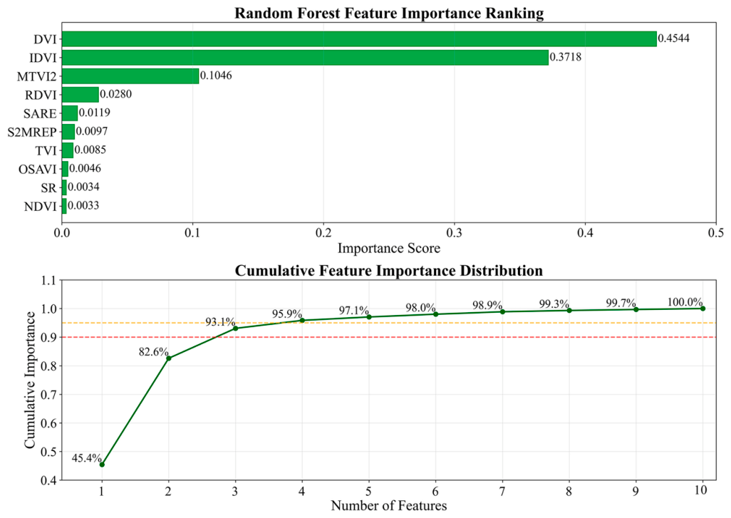
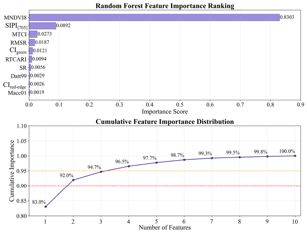
Subsequently, a model-driven ranking was applied to the pre-screened indices. Random forest regressors were employed to derive feature importance scores for both LAI and CCC. As illustrated in Figure 2 and Figure 3, both individual importance and cumulative contributions were examined. For LAI, the top-ranked indices (DVI and IDVI) accounted for more than 80% of the total importance, whereas for CCC, MNDVI8 emerged as the most influential predictor. By integrating collinearity analysis with importance rankings, highly redundant variables were removed while the five most informative indices for each target were retained. The final feature set (Table 5) thus provides a balanced multidimensional representation, combining 50 spectral bands with five optimized vegetation indices to support subsequent deep learning modeling.

2.5. Framework for Model Development and Transfer Learning

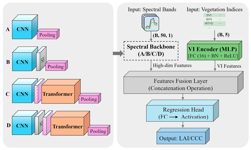
A deep learning framework integrating spectral feature modeling, transfer learning, and physical prior optimization was developed to systematically investigate simulation to reality crop trait retrieval. The framework evaluates three aspects: (i) the influence of network architecture complexity on spectral feature extraction and cross-domain generalization, (ii) the impact of physical prior quality on model transferability and predictive accuracy, and (iii) the effectiveness of transfer learning in mitigating the domain gap between simulated and in situ observations. Accordingly, the framework comprises three components: a dual-branch CNN–Transformer architecture with several baseline models for comparative analysis, a unified progressive transfer learning strategy for simulation to reality adaptation, and two PROSAIL-D simulation datasets with distinct levels of physical fidelity for assessing physical prior effects. For consistency in subsequent analyses, the proposed CNN–Transformer model is denoted as Model C, while Models A, B, and D are used as baselines for ablation studies.

2.5.1. Proposed CNN–Transformer Architecture

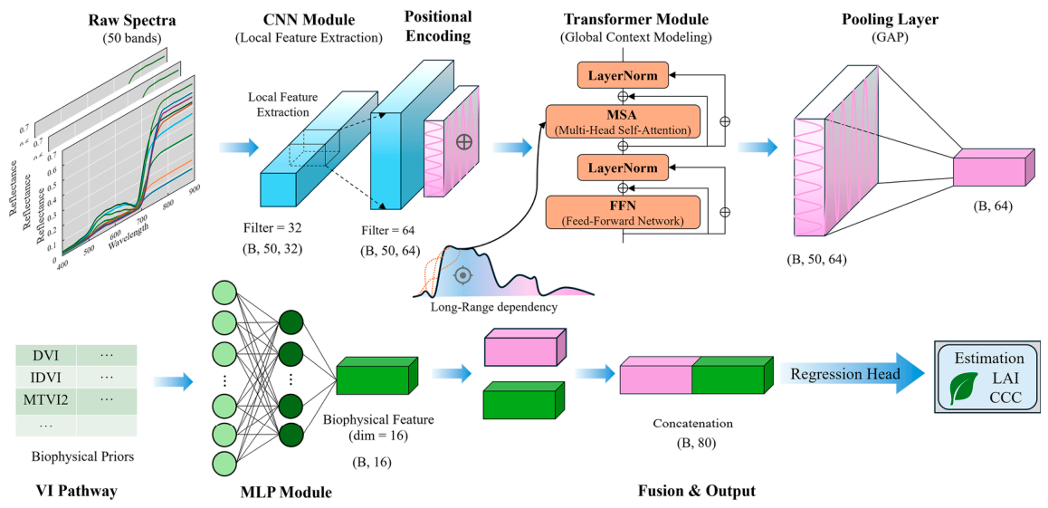
The proposed framework integrates continuous spectral information with physiologically meaningful vegetation indices, enabling joint exploitation of data-driven spectral representations and expert-informed biophysical descriptors for winter wheat. As illustrated in Figure 4, the model consists of a spectral branch, a vegetation-index branch, a feature fusion module, and a regression head. The spectral branch processes the 50-band hyperspectral sequence (400–890 nm) and serves as the primary feature extraction pathway. Two stacked one-dimensional convolutional layers with 32 and 64 filters, respectively, are first applied to extract local spectral structures, including absorption features, reflectance peaks, and inter-band interactions. Both layers use a kernel size of 3 and are followed by batch normalization and ReLU activation to improve training stability and nonlinear representational capacity.
To extend the receptive field beyond local convolution, learnable positional encodings are added to the extracted feature maps prior to input to the Transformer encoder. The encoder comprises four attention heads and a feed-forward network with a hidden dimension of 128. Through self-attention, global dependencies among spectrally distant wavelengths are modeled, complementing the local feature extraction capability of the CNN backbone. In parallel, a vegetation-index branch processes five selected hyperspectral-derived vegetation indices. This branch employs a lightweight multilayer perceptron with a fully connected layer of 16 neurons, followed by batch normalization and ReLU activation. It projects handcrafted indices into a latent feature space while preserving their physiological interpretability. The outputs of the two branches are concatenated and passed to a regression head consisting of a 64-neuron fully connected layer and a linear output layer.

2.5.2. Comparative Models for Ablation Analysis

To quantify the contribution of individual architectural components and evaluate the impact of model complexity on crop trait retrieval, three controlled baselines were constructed. The design isolates local convolution, channel attention, and global self-attention under identical input data and training configurations. Model A (CNN) is a pure one-dimensional convolutional network and serves as the baseline for local spectral feature extraction. Model B (CNN–SE) extends Model A by introducing a Squeeze-and-Excitation (SE) module to enable adaptive recalibration of channel-wise feature responses. Model D (CNN–SE–Transformer) integrates SE-based channel attention and Transformer-based global self-attention, representing the most complex configuration in this study. It is used to assess whether increased architectural complexity yields consistent performance gains or leads to redundancy and diminishing returns. For fair comparison, all models adopt identical dual-branch inputs (spectral bands and vegetation indices). Uniform preprocessing, identical optimization settings, and the same progressive transfer learning strategy are applied across all architectures. The overall framework of the proposed model and baselines is illustrated in Figure 5.

2.5.3. Unified Progressive Transfer Learning Strategy

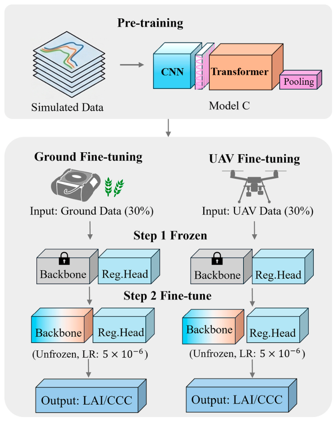
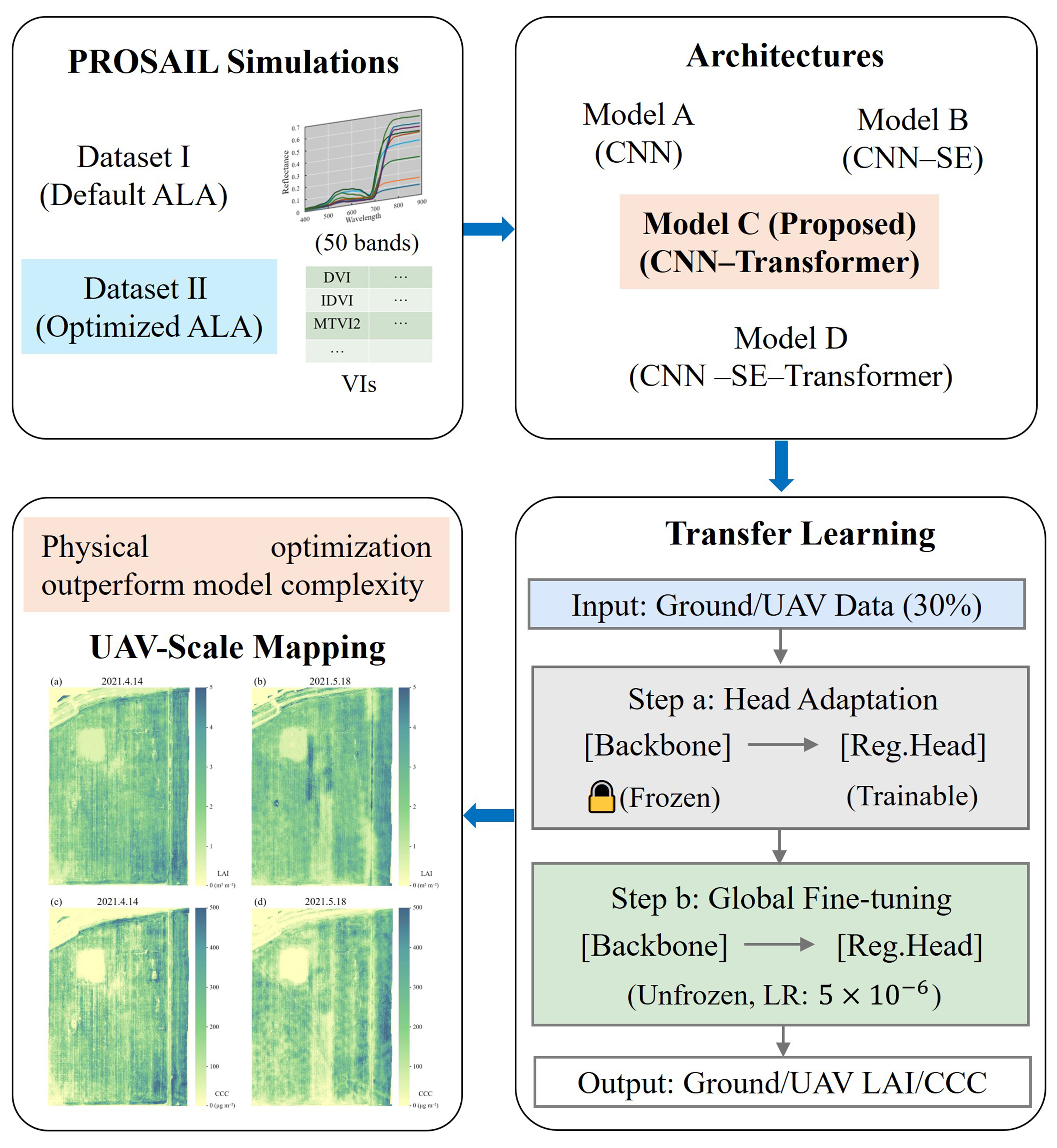
To mitigate the simulation to reality domain gap and improve generalization under limited field observations, a unified progressive transfer learning strategy was developed (Figure 6) and applied consistently across all candidate models to ensure a controlled comparison of architectural design and physical prior effects. The framework comprises two sequential stages: physics-informed pre-training and domain-adaptive fine-tuning. In the pre-training stage, all models are initialized using large-scale PROSAIL-D simulations (Datasets I and II), which provide physically consistent yet diverse canopy spectral responses under varying biophysical conditions. This stage enables learning of generalized radiative transfer relationships between spectral signals and crop traits, yielding physics-constrained parameter initialization. To enhance robustness to noise and outliers, the Huber loss (δ = 1.0) is adopted, and optimization is performed using Adam with an initial learning rate of 1 × 10⁻3.
Fine-tuning is conducted in two stages. In stage one (head adaptation), backbone parameters are frozen and only the regression head is updated, preserving physics-informed representations and reducing catastrophic forgetting under limited labeled data. In stage two (global fine-tuning), the full network is unfrozen and jointly optimized with a reduced learning rate of 5 × 10⁻6, enabling adaptation to domain-specific discrepancies, including sensor noise, atmospheric perturbations, and structural variability in ground-based and UAV observations, while maintaining pretrained physical consistency. A ReduceLROnPlateau scheduler (factor = 0.5) and early stopping are employed to stabilize convergence and prevent overfitting. This unified protocol is identically applied to all architectures and both simulation datasets, ensuring that performance differences arise solely from network structure and physical prior quality, rather than optimization settings.

2.6. Model Interpretability

To examine the internal decision mechanisms of the proposed framework and quantify the impact of physical prior optimization on feature utilization, SHAP were applied to attribute contributions of individual spectral bands and vegetation indices to model predictions. SHAP is a game-theoretic decomposition method that expresses model outputs as additive feature attributions and is widely used for interpreting complex machine learning models. The DeepSHAP variant was adopted for computational efficiency and compatibility with gradient-based neural networks. For an input sample x, the model prediction f(x) is expressed as:
f ( x )   =   ϕ 0   +   i   =   1 N ϕ i
where ϕ 0 represents the expected model output over a reference background dataset and ϕ i denotes the contribution of the i-th input feature to the final prediction.
SHAP analysis was performed on the fused feature representation, integrating outputs from the spectral and vegetation-index branches, enabling interpretation of the full model rather than isolated submodules. For each model, a background set of 200 randomly sampled training instances was used to estimate the expected output. SHAP values were computed using the DeepSHAP implementation in the SHAP library with 100 Monte Carlo forward passes to improve attribution stability, and final importance scores were obtained by averaging results across passes. Analyses were conducted separately for spectral bands (400–890 nm, 10 nm interval) and selected vegetation indices. To assess the effect of physical prior optimization, SHAP distributions were compared between models pretrained on Dataset I and Dataset II. Each experiment was repeated five times with different random seeds, and results were reported as averaged SHAP importance distributions. The resulting attribution maps were used to identify dominant spectral regions and vegetation indices for winter wheat LAI and CCC retrieval, and to evaluate whether physically optimized simulations promote more physiologically consistent feature utilization patterns.

2.7. Evaluation Metrics

The performance of all models was evaluated using the coefficient of determination (R2) and root mean square error (RMSE):
R 2   =   1   i   =   1 n ( y i   y ^ i ) 2 / i   =   1 n ( y i   y ¯ ) 2
R M S E = 1 n i = 1 n ( y i y ^ i ) 2
where y i , y ^ i , and y ¯ represent the observed value, predicted value, and mean observed value, respectively, and n denotes the number of samples. These metrics were calculated independently for winter wheat LAI and CCC retrieval under both ground-based hyperspectral observations and UAV hyperspectral images.

3. Results

3.1. Performance Comparison of Candidate Models

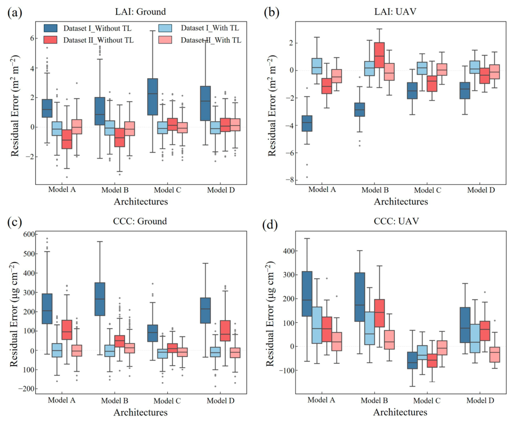
The performance of four candidate architectures (Models A–D) was systematically evaluated for winter wheat LAI and CCC retrieval using ground-based and UAV observations under two simulation datasets and two training strategies. Quantitative results are reported in Table 6 in terms of R2 and RMSE, while Figure 7 provides the corresponding residual distributions, offering complementary insight into model stability and predictive uncertainty. Overall, Table 6 and Figure 7 consistently indicate that Model C exhibits superior stability and robust performance across the vast majority of scenarios. Specifically, under the transfer learning framework on Dataset II, it yields peak ground-based retrieval accuracies for both LAI (R2 = 0.55, RMSE = 0.63) and CCC (R2 = 0.59, RMSE = 36.12 μg cm⁻2). Furthermore, cross-platform validation confirms strong UAV generalization capabilities, achieving reliable estimations for LAI (R2 = 0.53, RMSE = 0.62) and CCC (R2 = 0.59, RMSE = 37.56 μg cm⁻2). Correspondingly, Figure 7 shows the most compact residual distributions for Model C, with minimal dispersion and negligible bias across platforms. Relative to Model A and Model B, Model C reduces both error magnitude and variance. UAV LAI predictions from Model A exhibit wide dispersion and systematic negative bias (Figure 7c), whereas Model C produces near-zero-centered residuals with markedly reduced spread (Figure 7d). Similar trends are observed for CCC retrieval, where Model C achieves lower RMSE, indicating improved feature representation. Performance gains stem from the complementary structure of the CNN–Transformer architecture, where convolutional layers extract local spectral absorption features and the Transformer captures long-range dependencies across spectral regions such as the red-edge and NIR. In contrast, Model D does not further improve performance, showing comparable RMSE and similar residual patterns in Figure 7, suggesting diminishing returns from additional attention modules.

3.2. Effectiveness of Transfer Learning

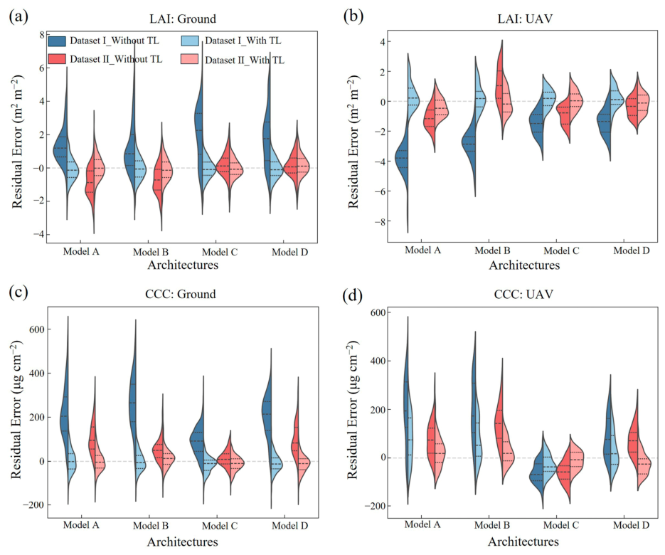
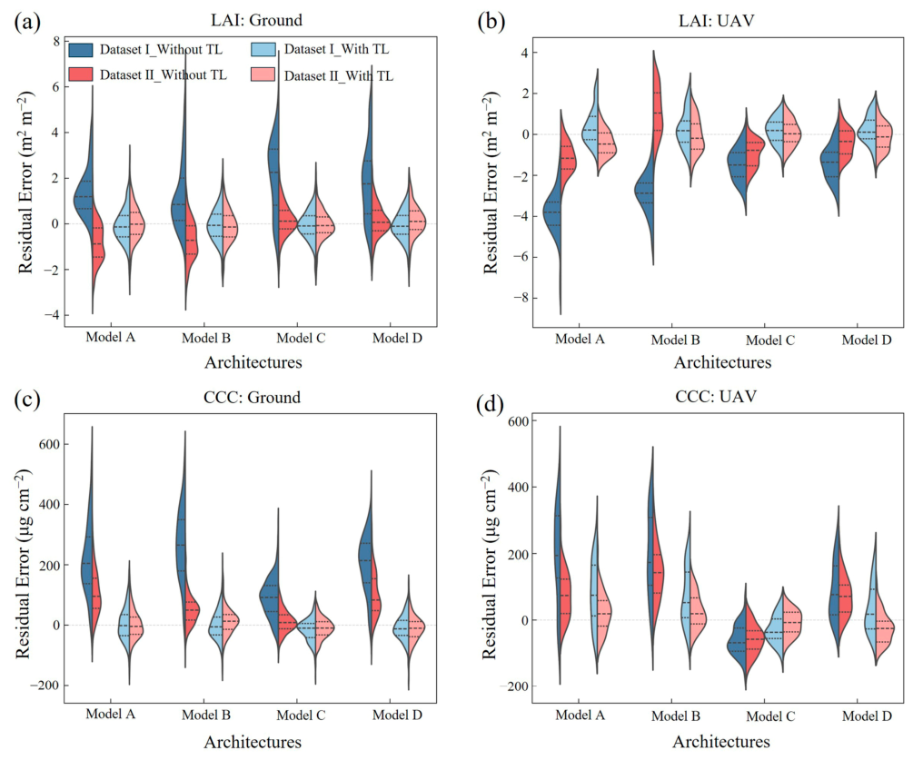
Figure 8 illustrates residual distributions of winter wheat LAI and CCC retrieval across four architectures, two datasets, two observation platforms, and two training strategies. Across all configurations, a consistent pattern emerges: transfer learning reduces both bias and variance of prediction errors. Under without TL settings, all models exhibit broad residual dispersion and systematic deviation from zero, with the most severe degradation observed in UAV-based retrievals due to pronounced domain shift. Applying TL consistently compresses residual distributions toward zero and improves symmetry, indicating improved alignment between simulated pretraining and real-world spectral characteristics. This effect is most evident in UAV scenarios, where without TL models show strongly skewed error distributions, reflecting substantial simulation to reality mismatch. After fine-tuning, dispersion is markedly reduced across all architectures. The improvement is consistent for both LAI and CCC, indicating that TL provides a task-agnostic adaptation mechanism rather than being architecture- or parameter-specific. Overall, Figure 8 demonstrates that transfer learning is essential for stabilizing model behavior under real-world deployment conditions, particularly in UAV-based and high-heterogeneity environments.
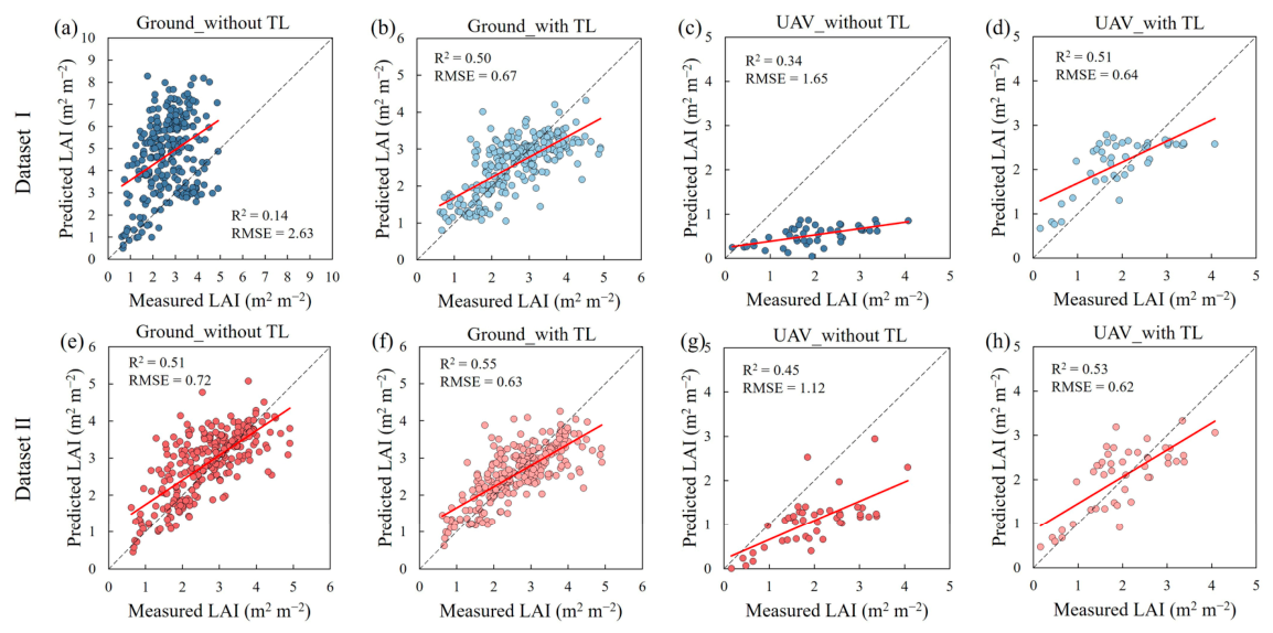
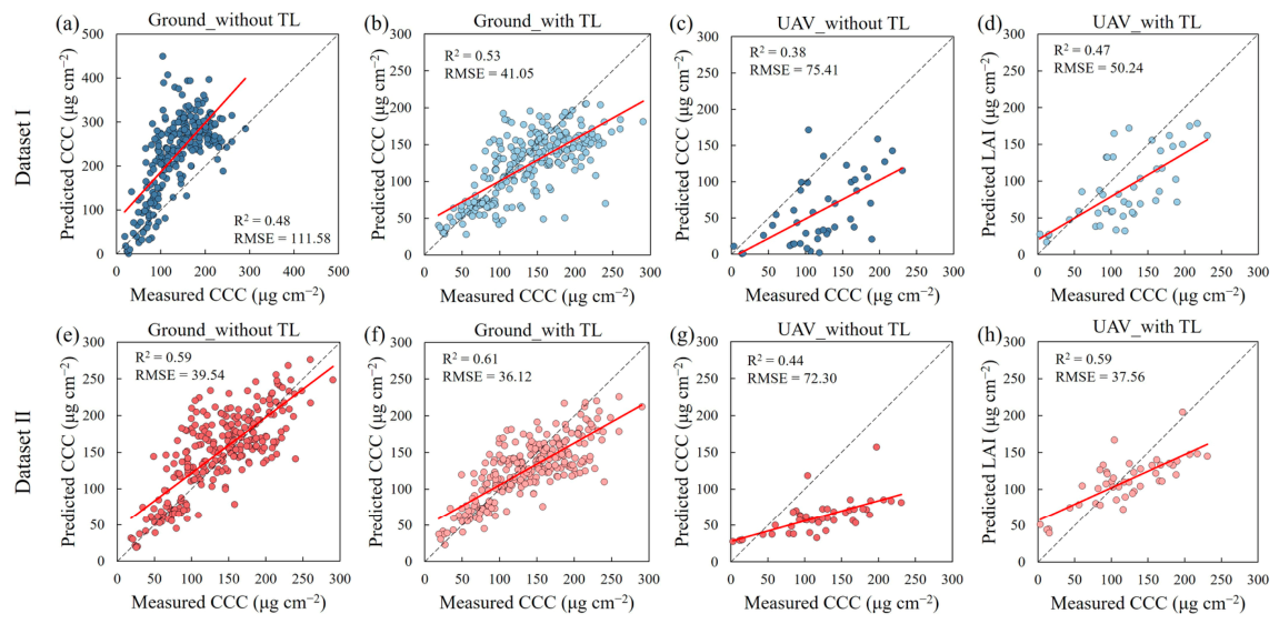
Figure 9 and Figure 10 further evaluate the optimal Model C using measured and predicted comparisons for LAI and CCC. For LAI (Figure 9), without TL configurations show clear deviations from the 1:1 line, with systematic underestimation in low-LAI regimes, especially under UAV observations. This reflects insufficient adaptation to complex canopy–sensor interactions. After TL, predictions align more closely with observations, with data points tightly distributed around the 1:1 reference line, indicating improved calibration of the spectral–biophysical mapping. A similar behavior is observed for CCC (Figure 10). Without TL, predictions exhibit increased scatter and pronounced bias, particularly in high-CCC regions, where errors are amplified due to domain inconsistency between RTM simulations and real canopy optical properties. With TL, predictions converge toward the 1:1 line, accompanied by a substantial reduction in RMSE. Bias in high-value ranges is notably suppressed, indicating improved sensitivity to physiologically critical variations.

3.3. Impact of Physical Prior Optimization

To assess the role of physical prior quality in cross-domain crop trait retrieval, this section combines regression diagnostics (Figure 9 and Figure 10) with residual analysis (Figure 11) to evaluate its impact on model generalization and error characteristics. Figure 9 and Figure 10 show measured–predicted relationships for LAI and CCC using Model C under different pretraining datasets and training strategies. Across both variables, increased physical realism in the pretraining data improves prediction consistency, even prior to transfer learning. With Dataset I, Model C deviates from the 1:1 line, particularly under UAV observations, where spectral heterogeneity leads to LAI underestimation at high values and increased CCC dispersion. These patterns indicate that imperfect RTM assumptions induce biased feature representations that propagate into prediction errors. In contrast, Dataset II yields a more compact regression structure, with predictions closely aligned to the 1:1 line and reduced heteroscedasticity for both LAI and CCC. This improvement is consistent across ground and UAV observations, indicating enhanced stability of learned spectral–biophysical mappings. The effect persists under both without and with TL settings, suggesting that physical prior quality constrains the upper performance bound independently of downstream adaptation.
Figure 11 further quantifies residual distributions across Models A–D, datasets, and training strategies. Dataset II consistently reduces both bias and variance, producing residuals that are more centered and narrowly distributed than Dataset I. The improvement is most pronounced under UAV observations, where Dataset I exhibits asymmetric and heavy-tailed residuals, particularly for CCC retrieval, reflecting structural mismatch between simulated and real canopy conditions. These distortions are substantially mitigated under Dataset II, yielding more symmetric and compact error distributions across all models. Improvements induced by physical optimization are consistent across architectures, indicating architecture-independent effects. Even for Model C, Dataset II produces substantially lower residual dispersion than Dataset I, demonstrating that model complexity alone cannot compensate for deficiencies in simulation physical fidelity.

3.4. Model Interpretation and UAV-Scale Spatial Mapping

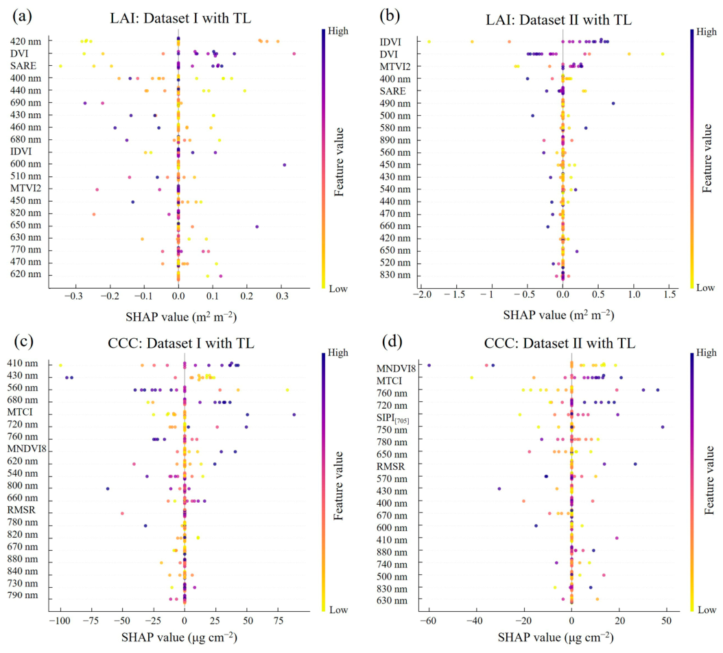
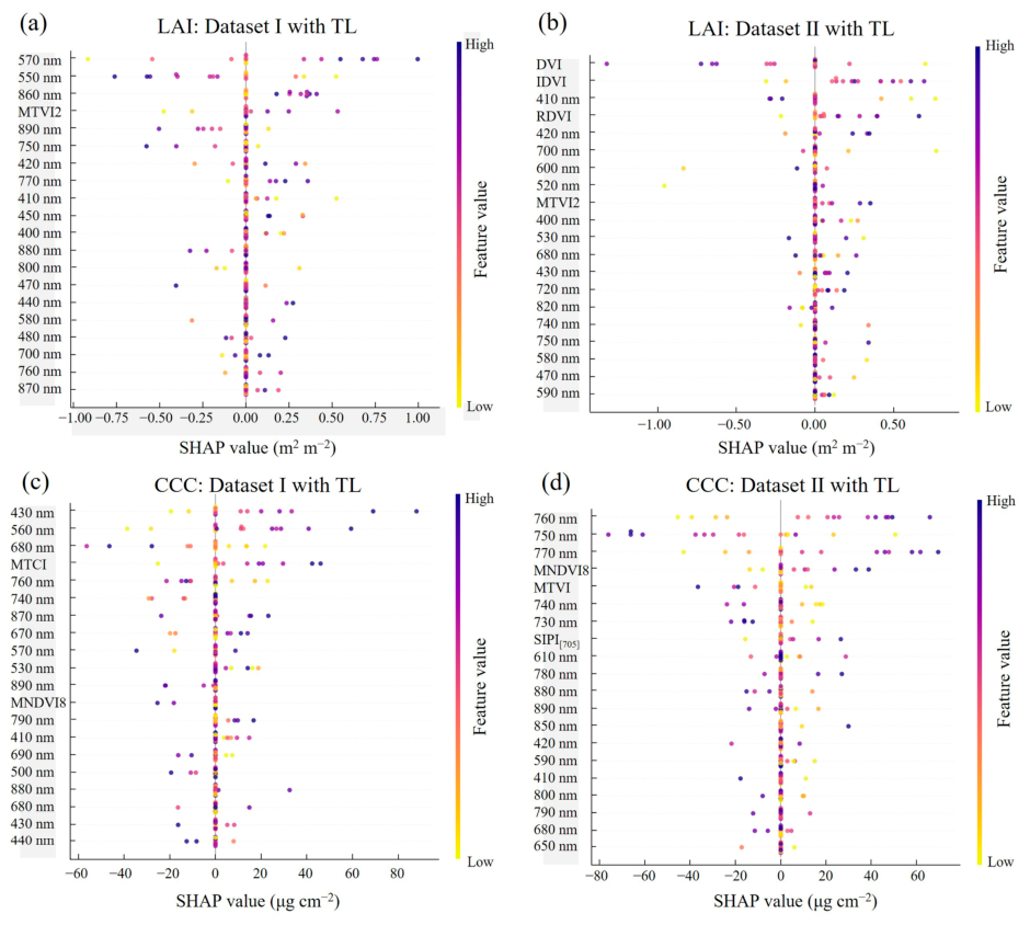
Figure 12 presents the global SHAP feature importance distributions of the proposed model under different pre-training datasets with TL, evaluated on UAV observations for LAI and CCC retrieval. For LAI retrieval, under Dataset I with TL (Figure 12a), feature attribution was mainly distributed across visible wavelengths (e.g., 400–470 nm) and several vegetation indices, including DVI and SARE. In contrast, Dataset II with TL (Figure 12b) shifted feature importance toward physiologically meaningful variables, particularly IDVI, DVI, and MTVI2, while reducing dependence on isolated spectral bands. This indicates that physically optimized simulations promoted more structured and biophysically consistent feature representations. For CCC retrieval, Dataset I with TL (Figure 12c) exhibited dispersed feature contributions across visible and mixed spectral regions, suggesting weaker physiological consistency. After physical optimization, Dataset II with TL (Figure 12d) showed enhanced contributions from red-edge and near-infrared wavelengths (e.g., 720–780 nm) and chlorophyll-sensitive indices, including MTCI, MNDVI8, and SIPI [705]. These results demonstrate that physical prior optimization systematically reshaped model attribution patterns by encouraging reliance on stable spectral–biophysical relationships rather than unstable spectral correlations.
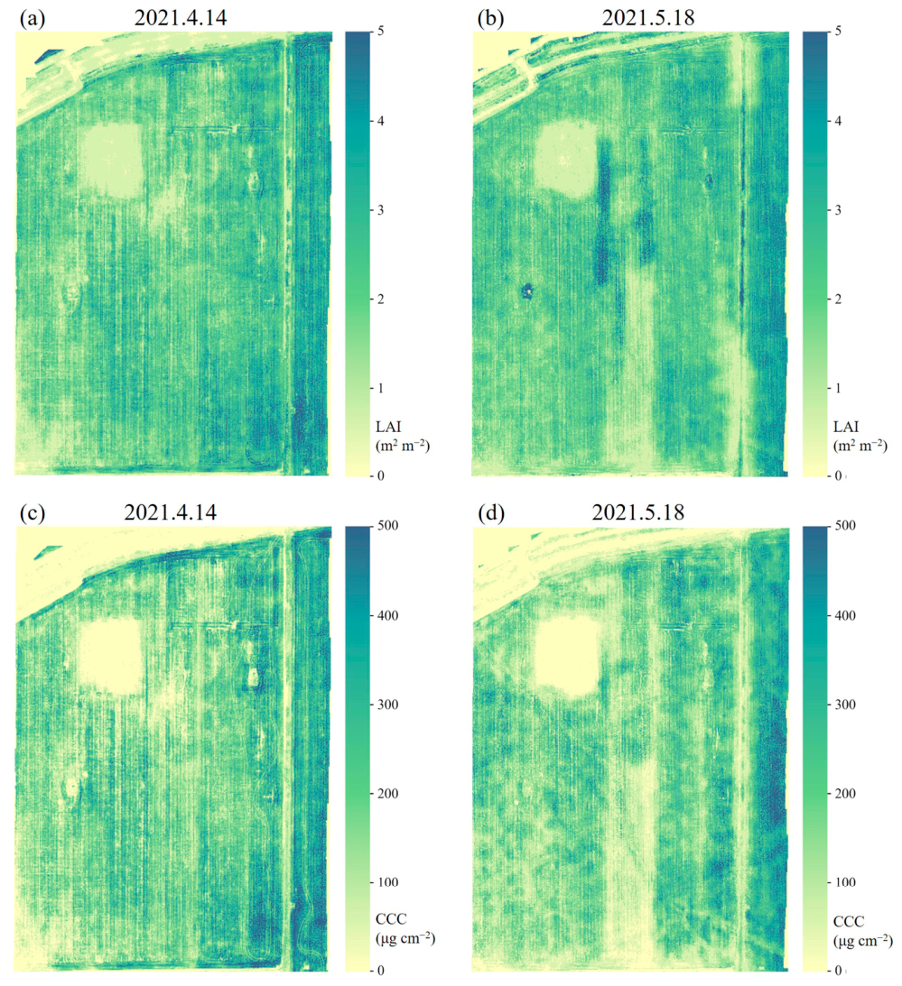
To further evaluate the practical applicability of the proposed framework at the UAV observation scale, pixel-wise retrieval was performed using UAV hyperspectral imagery collected over the winter wheat field. The proposed CNN–Transformer model pretrained with Dataset II and adapted through transfer learning was applied to generate spatial distributions of LAI and CCC (Figure 13). The retrieved maps revealed clear spatial heterogeneity in crop canopy structure and physiological status, reflecting variations in field growth conditions. The LAI map showed continuous spatial patterns associated with canopy density differences, whereas the CCC map exhibited similar but physiologically distinct spatial variations related to chlorophyll accumulation. Compared with discrete ground measurements, UAV-based mapping provides spatially explicit information, demonstrating the capability of the proposed framework for extending trait retrieval from plot-level estimation to field-scale monitoring. These results further confirm that physically optimized simulation and transfer learning enable robust deployment of hyperspectral deep learning models under operational agricultural remote sensing scenarios.

4. Discussion

4.1. Transfer Learning as the Essential Bridge Between Simulation and Reality

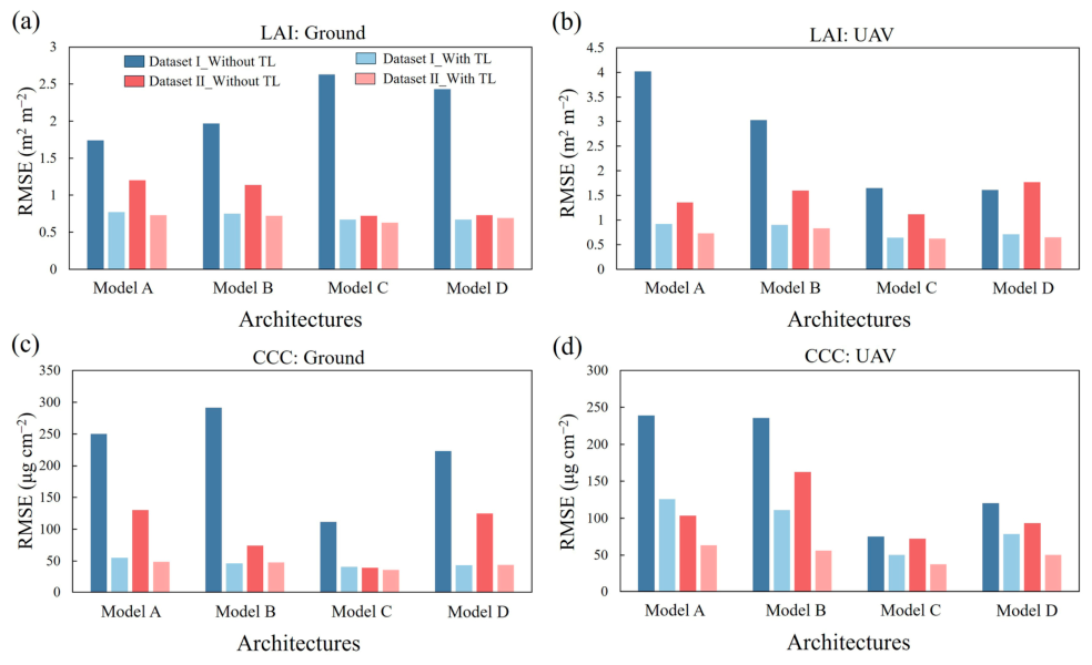
Deep learning models trained on radiative transfer model (RTM) simulations, particularly PROSAIL-based synthetic datasets, have been widely adopted to alleviate limited field observations in crop trait retrieval [13,22,52,53]. However, most studies implicitly assume negligible distributional discrepancy between simulated and real spectra, an assumption rarely satisfied in practice. The results in Figure 14 directly contradict this assumption. Models trained solely on simulated data show substantial performance degradation when applied to real observations, with the strongest deterioration observed in UAV scenarios due to amplified scale effects and sensor noise. This behavior is consistent with reported domain shift issues in hyperspectral retrieval [27,54] and further extends prior findings by quantifying failure patterns across both LAI and CCC tasks. This degradation is primarily driven by inconsistencies between idealized RTM assumptions (e.g., homogeneous canopy structure and simplified atmospheric effects) and real canopy complexity. Transfer learning mitigates this mismatch by decoupling physics-based representation learning in the simulation domain from domain-specific calibration using limited field data. This two-stage paradigm preserves physically meaningful spectral–biophysical relationships while adapting to sensor- and environment-induced variations. These results indicate that transfer learning is not merely a performance enhancement strategy but a necessary condition for stable simulation to reality crop trait retrieval.

4.2. Physical Fidelity as the Dominant Factor in Generalization Performance

A persistent debate in remote sensing concerns whether performance gains should be driven by increasingly complex deep learning architectures or by improved physical realism in training data. Although advanced architectures such as attention-based networks and hybrid CNN–Transformer models are widely used [24,55,56], their benefits under limited-sample transfer settings remain unstable. The results indicate that physical fidelity of simulated data exerts a stronger and more consistent influence on generalization than architectural complexity. In particular, optimization of leaf angle distribution substantially reduces systematic errors prior to transfer learning, as evidenced by the contrast between Dataset I and Dataset II in Figure 14. This suggests that a substantial portion of prediction error originates from biased physical priors embedded in the simulation process rather than from limitations of the learning architecture. From a mechanistic perspective, low-fidelity simulations force the network to learn compensatory mappings that encode structural bias rather than true radiative transfer behavior. In contrast, physically consistent simulations reduce this representational mismatch, allowing transfer learning to focus on residual stochastic variability instead of correcting fundamental physical inconsistencies. These findings challenge the common assumption that improved retrieval accuracy is primarily driven by more expressive neural architectures. Instead, the results indicate that performance is fundamentally constrained by data physics, which defines the upper bound of generalization, while model refinement provides only secondary gains.

4.3. Physical Priors Reshape Feature Learning and Improve Cross-Scale Consistency

Beyond predictive accuracy, recent studies emphasize interpretability and reliability as key requirements for deep learning in remote sensing retrieval [57,58,59]. However, the mechanism by which physical priors influence internal feature selection across observation scales remains insufficiently understood. In this study, SHAP-based attribution analysis reveals a clear behavioral divergence between models trained on default and physically optimized simulations. Models trained with default simulations exhibit strong dependence on volatile visible bands (400–450 nm), a spectral region highly sensitive to atmospheric scattering and soil background effects. This indicates that the network relies on spurious correlations rather than stable biophysical relationships. In contrast, physically optimized priors systematically reconfigure feature attribution, shifting importance toward red-edge and near-infrared wavelengths and vegetation indices sensitive to chlorophyll content and canopy structure. This feature migration is consistent across ground-based (Figure 15) and UAV observations (Figure 12), indicating improved cross-scale stability. These results suggest that physical priors function as an implicit domain regularizer during representation learning by correcting systematic biases in synthetic data and constraining the hypothesis space toward physiologically meaningful mappings. Unlike architectural modifications such as attention or Transformer modules, which primarily adjust model capacity, physical prior optimization directly reshapes the input–output mapping structure. This yields a more favorable balance between predictive robustness and interpretability, providing a scalable framework for cross-scale crop trait retrieval.

4.4. Limitations and Future Perspectives

Despite the strong performance of the proposed framework, several limitations remain. First, the study is restricted to winter wheat in a specific agroecological region, which limits its transferability to crops with different canopy structures and radiative properties. Multi-crop validation is required to assess the generality of the physical optimization strategy. Second, only leaf angle distribution was modified in the simulation pipeline. Canopy radiative transfer is jointly controlled by multiple interacting factors, including leaf optical properties, soil background heterogeneity, and canopy clumping effects. The omission of these factors constrains the completeness of the physical prior formulation. Third, although transfer learning improves domain adaptation, the current framework remains deterministic and does not explicitly quantify predictive uncertainty, limiting its applicability in operational decision-support contexts requiring risk-aware outputs. Future work should extend physically constrained simulations to multi-parameter settings, develop physics-informed or domain-generalization learning frameworks, and incorporate uncertainty quantification techniques such as Bayesian deep learning or conformal prediction.

5. Conclusions

This study develops a unified framework for robust winter wheat LAI and CCC retrieval from ground-based and UAV hyperspectral observations by integrating physically constrained simulation, transfer learning, and deep neural architectures. Results demonstrate that physical optimization of radiative transfer simulations is the primary determinant of inversion robustness, as it mitigates systematic inductive bias at the source by incorporating realistic physical priors. Models trained solely on synthetic data exhibit severe performance degradation under real-world conditions, whereas progressive transfer learning with limited field observations effectively bridges the simulation to reality gap by aligning simulated feature distributions with empirical spectral characteristics. Under constrained data regimes, increasing architectural complexity yields diminishing returns; the CNN–Transformer model achieves the best balance between representation capacity and generalization, while more complex variants provide only marginal gains. SHAP-based attribution analysis further confirms that physical simulation optimization reshapes model interpretability, shifting feature dependence from unstable visible bands toward red-edge regions and physiologically meaningful vegetation indices. Overall, robust crop trait inversion follows a tripartite mechanism: physical realism sets the performance ceiling, transfer learning enables domain adaptation, and tailored network design improves representation efficiency. Future work will extend multi-parameter physical optimization and integrate uncertainty-aware learning frameworks to support large-scale operational agricultural monitoring.

Author Contributions

Conceptualization, Q.S. and Q.J.; methodology, Q.S. and Q.J.; software, Q.S. S.C. and S.Z.; validation, Q.S., Q.J. and S.C.; formal analysis, Q.S. and L.P.; investigation, Q.S., Q.J. and S.Z; resources, Q.J. and W.H.; data curation, Q.S. and L.P.; writing—original draft preparation, Q.S.; writing—review and editing, Q.J. and X.Z.; visualization, Q.S.; supervision, X.Z. and W.H.; project administration, X.Z. and W.H.; funding acquisition, Q.S. and Q.J. All authors have read and agreed to the published version of the manuscript.

Funding

This research was funded by the National Key R&D Program of China, grant number 2023YFB3906202 and the National Natural Science Foundation of China, grant number 32571914.

Data Availability Statement

The data supporting the results of this study can be obtained by contacting the corresponding author.

Acknowledgments

During the preparation of this manuscript, the authors used ChatGPT-5.5 (OpenAI) for language editing, improving manuscript readability, and providing suggestions on figure layout and color schemes. The authors have reviewed and edited the output and take full responsibility for the content of this publication.

Conflicts of Interest

The authors declare no conflicts of interest.

References

  1. Godfray, H.C.J.; Beddington, J.R.; Crute, I.R.; Haddad, L.; Lawrence, D.; Muir, J.F.; Pretty, J.; Robinson, S.; Thomas, S.M.; Toulmin, C. Food security: the challenge of feeding 9 billion people. Science 2010, 327, 812–818. [Google Scholar] [CrossRef] [PubMed]
  2. Ma, G.; Pincebourde, S.; Bai, X.; Peng, Y.; Wang, X.; Yang, H.; Zhu, L.; Zhang, W.; Ma, C. Behavioural plasticity of a pest species may aggravate global wheat yield loss under climate change. Nat. Commun. 2025, 16, 11163. [Google Scholar] [CrossRef] [PubMed]
  3. Mulla, D.J. Twenty five years of remote sensing in precision agriculture: Key advances and remaining knowledge gaps. Biosyst. Eng. 2013, 114, 358–371. [Google Scholar] [CrossRef]
  4. Chlingaryan, A.; Sukkarieh, S.; Whelan, B. Machine learning approaches for crop yield prediction and nitrogen status estimation in precision agriculture: A review. Comput. Electron. Agr. 2018, 151, 61–69. [Google Scholar] [CrossRef]
  5. Hashemi, M.G.Z.; Alemohammad, H.; Jalilvand, E.; Tan, P.N.; Judge, J.; Cosh, M.; Das, N.N. Estimating crop biophysical parameters from satellite-based SAR and optical observations using self-supervised learning with geospatial foundation models. Remote Sens. Environ. 2025, 327, 114825. [Google Scholar] [CrossRef]
  6. Maddonni, G.A.; Otegui, M.E. Leaf area, light interception, and crop development in maize. Field Crop. Res. 1996, 48, 81–87. [Google Scholar] [CrossRef]
  7. Luo, S.; Li, Q.; Du, L.; Wu, Z. Time-space-angle scale effects and incorporation patterns in estimating rice LAI and leaf chlorophyll content by UAV multispectral remote sensing. Comput. Electron. Agr. 2025, 237, 110792. [Google Scholar] [CrossRef]
  8. Wang, S.; Guan, K.; Wang, Z.; Ainsworth, E.A.; Zheng, T.; Townsend, P.A.; Li, K.; Moller, C.; Wu, G.; Jiang, C. Unique contributions of chlorophyll and nitrogen to predict crop photosynthetic capacity from leaf spectroscopy. J. Exp. Bot. 2021, 72, 341–354. [Google Scholar] [PubMed]
  9. Zhang, B.; Gu, L.; Dai, M.; Bao, X.; Sun, Q.; Zhang, M.; Qu, X.; Li, Z.; Zhen, W.; Gu, X. Estimation of grain filling rate of winter wheat using leaf chlorophyll and LAI extracted from UAV images. Field Crop. Res. 2024, 306, 109198. [Google Scholar] [CrossRef]
  10. Guo, X.; Wang, R.; Chen, J.M.; Cheng, Z.; Zeng, H.; Miao, G.; Huang, Z.; Guo, Z.; Cao, J.; Niu, J. Synergetic inversion of leaf area index and leaf chlorophyll content using multi-spectral remote sensing data. Geo-Spat. Inf. Sci. 2025, 28, 22–35. [Google Scholar]
  11. Xie, Q.; Dash, J.; Huete, A.; Jiang, A.; Yin, G.; Ding, Y.; Peng, D.; Hall, C.C.; Brown, L.; Shi, Y.; Ye, H.; Dong, Y.; Huang, W. Retrieval of crop biophysical parameters from Sentinel-2 remote sensing imagery. Int. J. Appl. Earth Obs. 2019, 80, 187–195. [Google Scholar] [CrossRef]
  12. Li, W.; Li, D.; Warner, T.A.; Liu, S.; Baret, F.; Yang, P.; Jiang, J.; Dong, M.; Cheng, T.; Zhu, Y.; Cao, W.; Yao, X. Improved generality of wheat green LAI models through mitigation of the effect of leaf chlorophyll content variation with red edge vegetation indices. Remote Sens. Environ. 2025, 318, 114589. [Google Scholar] [CrossRef]
  13. Verrelst, J.; Camps-Valls, G.; Muñoz-Marí, J.; Rivera, J.P.; Veroustraete, F.; Clevers, J.G.P.W.; Moreno, J. Optical remote sensing and the retrieval of terrestrial vegetation bio-geophysical properties—A review. ISPRS J. Photogramm. 2015, 108, 273–290. [Google Scholar] [CrossRef]
  14. Tian, Z.; Fan, J.; Yu, T.; Leon, N.D.; Kaeppler, S.M.; Zhang, Z. Mitigating NDVI saturation in imagery of dense and healthy vegetation. ISPRS J. Photogramm. 2025, 227, 234–250. [Google Scholar] [CrossRef]
  15. Porterie, M.; Martín, M.P.; Burchard-Levine, V.; González-Cascón, R.; Démoulin, R. Combining spectral libraries and 3D radiative transfer modeling to improve the simulation of phenology in semi-arid grasslands. IEEE J.-STARS. 2025, 18, 22441–22465. [Google Scholar] [CrossRef]
  16. Sun, Q.; Jiao, Q.; Chen, X.; Xing, H.; Huang, W.; Zhang, B. Machine learning algorithms for the retrieval of canopy chlorophyll content and leaf area index of crops using the PROSAIL-D model with the adjusted average leaf angle. Remote Sens. 2023, 15, 2264. [Google Scholar] [CrossRef]
  17. Brown, L.A.; Fernandes, R.; Verrelst, J.; Morris, H.; Djamai, N.; Reyes-Muñoz, P.; D.Kovács, D.; Meier, C. GROUNDED EO: Data-driven Sentinel-2 LAI and FAPAR retrieval using Gaussian processes trained with extensive fiducial reference measurements. Remote Sens. Environ. 2025, 326, 114797. [Google Scholar] [CrossRef]
  18. Verrelst, J.; García-Soria, J.L.; Reyes-Muñoz, P.; Clerck, E.D.; Morata, M.; Rivera-Caicedo, J.P. Epistemic and aleatoric uncertainty in optical vegetation trait retrieval: Concepts, Methods, and Outlook. ISPRS J. Photogramm. 2026, 234, 20–45. [Google Scholar] [CrossRef]
  19. Maya Gopal, P.S.; Bhargavi, R. Performance evaluation of best feature subsets for crop yield prediction using machine learning algorithms. Appl. Artif. Intell. 2019, 33, 621–642. [Google Scholar] [CrossRef]
  20. Abdel-salam, M.; Kumar, N.; Mahajan, S. A proposed framework for crop yield prediction using hybrid feature selection approach and optimized machine learning. Neural Comput. Appl. 2024, 36, 20723–20750. [Google Scholar] [CrossRef]
  21. Ball, J.E.; Anderson, D.T.; Chan, C. Comprehensive survey of deep learning in remote sensing: theories, tools, and challenges for the community. J. Appl. Remote Sens. 2017, 11, 042609. [Google Scholar] [CrossRef]
  22. Wang, D.; Cao, W.; Zhang, F.; Li, Z.; Xu, S.; Wu, X. A review of deep learning in multiscale agricultural sensing. Remote Sens. 2022, 14, 559. [Google Scholar] [CrossRef]
  23. Peng, M.; Liu, Y.; Khan, A.; Ahmed, B.; Sarker, S.K.; Ghadi, Y.Y.; Bhatti, U.A.; Al-Razgan, M.; Ali, Y.A. Crop monitoring using remote sensing land use and land change data: Comparative analysis of deep learning methods using pre-trained CNN models. Big Data Res. 2024, 36, 100448. [Google Scholar] [CrossRef]
  24. Zheng, G. Transformer-Based Sensor-Agnostic Model for Satellite Chlorophyll Retrieval. IEEE T. Geosci. Remote 2025, 63, 4405213. [Google Scholar] [CrossRef]
  25. Mienye, I.D.; Swart, T.G.; Obaido, G. Recurrent neural networks: A comprehensive review of architectures, variants, and applications. Information 2024, 15, 517. [Google Scholar] [CrossRef]
  26. Khan, S.A.; Martínez-de-Morentin, X.; Alsabbagh, A.R.; Maillo, A.; Lagani, V.; Gomez-Cabrero, D.; Lehmann, R.; Tegner, J. Multimodal foundation transformer models for multiscale genomics. Nat. Methods 2026, 23, 299–311. [Google Scholar] [PubMed]
  27. Skobalski, J.; Sagan, V.; Alifu, H.; Akkad, O.A.; Lopes, F.A.; Grignola, F. Bridging the gap between crop breeding and GeoAI: Soybean yield prediction from multispectral UAV images with transfer learning. ISPRS J. Photogramm. 2024, 210, 260–281. [Google Scholar] [CrossRef]
  28. Zhang, Y.; Hui, J.; Qin, Q.; Sun, Y.; Zhang, T.; Sun, H.; Li, M. Transfer-learning-based approach for leaf chlorophyll content estimation of winter wheat from hyperspectral data. Remote Sens. Environ. 2021, 267, 112724. [Google Scholar] [CrossRef]
  29. Li, J.; Xiao, Z.; Sun, R.; Song, J. A method to estimate leaf area index from VIIRS surface reflectance using deep transfer learning. ISPRS J. Photogramm. 2023, 202, 512–527. [Google Scholar] [CrossRef]
  30. Porra, R.J. The chequered history of the development and use of simultaneous equations for the accurate determination of chlorophylls a and b. Photosynth. Res. 2002, 73, 149–156. [Google Scholar] [CrossRef] [PubMed]
  31. Féret, J.B.; Gitelson, A.A.; Noble, S.D.; Jacquemoud, S. PROSPECT-D: Towards modeling leaf optical properties through a complete lifecycle. Remote Sens. Environ. 2017, 193, 204–215. [Google Scholar] [CrossRef]
  32. Verhoef, W.; Jia, L.; Xiao, Q.; Su, Z. Unified optical-thermal four-stream radiative transfer theory for homogeneous vegetation canopies. IEEE T. Geosci. Remote 2007, 45, 1808–1822. [Google Scholar] [CrossRef]
  33. Verhoef, W. Theory of Radiative Transfer Models Applied in Optical Remote Sensing of Vegetation Canopies. Ph.D. Thesis, Wageningen Agricultural University, Wageningen, The Netherlands, 1998. [Google Scholar]
  34. Jiao, Q.; Sun, Q.; Zhang, B.; Huang, W.; Ye, H.; Zhang, Z.; Zhang, X.; Qian, B. A random forest algorithm for retrieving canopy chlorophyll content of wheat and soybean trained with PROSAIL simulations using adjusted average leaf angle. Remote Sens. 2021, 14, 98. [Google Scholar] [CrossRef]
  35. Rouse, J.W.; Haas, R.H., Jr.; Schell, J.A.; Deering, D.W. Monitoring vegetation systems in the Great Plains with ERTS. In NASA SP-351 Third ERTS-1 Symposium; Fraden, S.C., Marcanti, E.P., Becker, M.A., Eds.; Scientific and Technical Information Office, National Aeronautics and Space Administration: Washington, DC, USA, 1974; pp. 309–317. [Google Scholar]
  36. Richardson, A.J.; Weigand, C.L. Distinguishing vegetation from soil background information. Photogramm. Eng. Rem. S. 1977, 43, 1541–1552. [Google Scholar]
  37. Roujean, J.L.; Breon, F.M. Estimating PAR absorbed by vegetation from bidirectional reflectance measurements. Remote Sens. Environ. 1995, 51, 375–384. [Google Scholar] [CrossRef]
  38. Haboudane, D.; Miller, J.R.; Pattey, E.; Zarco-Tejada, P.J.; Strachan, I.B. Hyperspectral vegetation indices and novel algorithms for predicting green LAI of crop canopies: Modeling and validation in the context of precision agriculture. Remote Sens. Environ. 2004, 90, 337–352. [Google Scholar] [CrossRef]
  39. Rondeaux, G.; Steven, M.; Baret, F. Optimization of soil-adjusted vegetation indices. Remote Sens. Environ. 1996, 55, 95–107. [Google Scholar] [CrossRef]
  40. Sun, Y.; Ren, H.; Zhang, T.; Zhang, C.; Qin, Q. Crop leaf area index retrieval based on inverted difference vegetation index and NDVI. IEEE Geosci. Remote S. 2018, 15, 1662–1666. [Google Scholar] [CrossRef]
  41. Ali, M.; Montzka, C.; Stadler, A.; Menz, G.; Thonfeld, F.; Vereecken, H. Estimation and validation of RapidEye-based time-series of leaf area index for winter wheat in the Rur catchment (Germany). Remote Sens. 2015, 7, 2808–2831. [Google Scholar] [CrossRef]
  42. Broge, N.H.; Leblanc, E. Comparing prediction power and stability of broadband and hyperspectral vegetation indices for estimation of green leaf area index and canopy chlorophyll density. Remote Sens. Environ. 2001, 76, 156–172. [Google Scholar] [CrossRef]
  43. Jordan, C.F. Derivation of leaf-area index from quality of light on the forest floor. Ecology 1969, 50, 663–666. [Google Scholar] [CrossRef]
  44. Dash, J.; Curran, P.J. The MERIS terrestrial chlorophyll index. Int. J. Remote Sens. 2004, 25, 5403–5413. [Google Scholar] [CrossRef]
  45. Wu, C.; Niu, Z.; Tang, Q.; Huang, W. Estimating chlorophyll content from hyperspectral vegetation indices: Modeling and validation. Agr. For. Meteorol. 2008, 148, 1230–1241. [Google Scholar] [CrossRef]
  46. Gitelson, A.A.; Gritz, Y.; Merzlyak, M.N. Relationships between leaf chlorophyll content and spectral reflectance and algorithms for non-destructive chlorophyll assessment in higher plant leaves. J. Plant Physiol. 2003, 160, 271–282. [Google Scholar] [CrossRef] [PubMed]
  47. Gitelson, A.A.; Keydan, G.P.; Merzlyak, M.N. Three-band model for noninvasive estimation of chlorophyll, carotenoids, and anthocyanin contents in higher plant leaves. Geophys. Res. Lett. 2006, 33, L11402. [Google Scholar] [CrossRef]
  48. Mutanga, O.; Skidmore, A.K. Narrow band vegetation indices overcome the saturation problem in biomass estimation. Int. J. Remote Sens. 2004, 25, 3999–4014. [Google Scholar] [CrossRef]
  49. Penuelas, J.; Baret, F.; Filella, I. Semi-empirical indices to assess carotenoids/chlorophyll a ratio from leaf spectral reflectance. Photosynthetica 1995, 31, 221–230. [Google Scholar]
  50. Maccioni, A.; Agati, G.; Mazzinghi, P. New vegetation indices for remote measurement of chlorophylls based on leaf directional reflectance spectra. J. Photoch. Photobio. B. 2001, 61, 52–61. [Google Scholar] [CrossRef] [PubMed]
  51. Datt, B. Visible/near infrared reflectance and chlorophyll content in Eucalyptus leaves. Int. J. Remote Sens. 1999, 20, 2741–2759. [Google Scholar] [CrossRef]
  52. Yang, B.; Zhou, L.; Yang, G.; Zhang, G.; Qi, J.; Li, C. Integrating hyperspectral radiation transfer modeling and deep transfer learning to estimate nitrogen density in winter wheat canopies. Artif. Intell. Agr. 2026, 16, 753–763. [Google Scholar] [CrossRef]
  53. Zhang, P.; Lu, B.; Shang, J.; Shen, S.; Ge, J.; Wang, X.; Sun, S.; Yang, Y.; Zang, H.; Zeng, Z. PROSAIL-DNN: a fine-tuning transfer learning framework for field-scale oat leaf area index monitoring from UAV imagery. Comput. Electron. Agr. 2026, 241, 111272. [Google Scholar] [CrossRef]
  54. Du, R.; Shi, W.; Lu, X.; Xiang, Y.; Zhang, Y.; Feng, X.; Ma, Y. TrSC2Y: A transfer-learning-based model from UAV hyper-spectra imagery for field-scale canola yield prediction by integrating DSSAT with PROSAIL. Eur. J. Agron. 2026, 174, 127926. [Google Scholar] [CrossRef]
  55. Du, J.; Zhang, Y.; Wang, P.; Tansey, K.; Liu, J.; Zhang, S. Enhancing winter wheat yield estimation with a CNN-transformer hybrid framework utilizing multiple remotely sensed parameters. IEEE T. Geosci. Remote 2025, 63, 4405213. [Google Scholar] [CrossRef]
  56. Liu, L.; Xie, Y.; Zhu, B.; Song, K. A Deep Learning Model Combining CNN and Transformer for Rice Yield Estimation at County and Pixel Scales in Northeast China. IEEE J.-STARS. 2026, 19, 13927–13959. [Google Scholar] [CrossRef]
  57. Descals, A.; Verger, A.; Yin, G.; Filella, I.; Peñuelas, J. Local interpretation of machine learning models in remote sensing with SHAP: the case of global climate constraints on photosynthesis phenology. Int. J. Remote Sens. 2023, 44, 3160–3173. [Google Scholar] [CrossRef]
  58. Zeng, X.; Han, D.; Tansey, K.; Wang, P.; Pei, M.; Li, Y.; Li, F.; Du, Y. An interpretable wheat yield estimation model using time series remote sensing data and considering meteorological and soil influences. Remote Sens. 2025, 17, 3192. [Google Scholar] [CrossRef]
  59. Hu, Y.; Zhan, W.; He, Q.; Liu, Y.; Zhan, H. A spatially-informed interpretable deep learning framework for high-resolution nutrient monitoring in complex coastal waters. Int. J. Appl. Earth Obs. 2026, 146, 105025. [Google Scholar] [CrossRef]
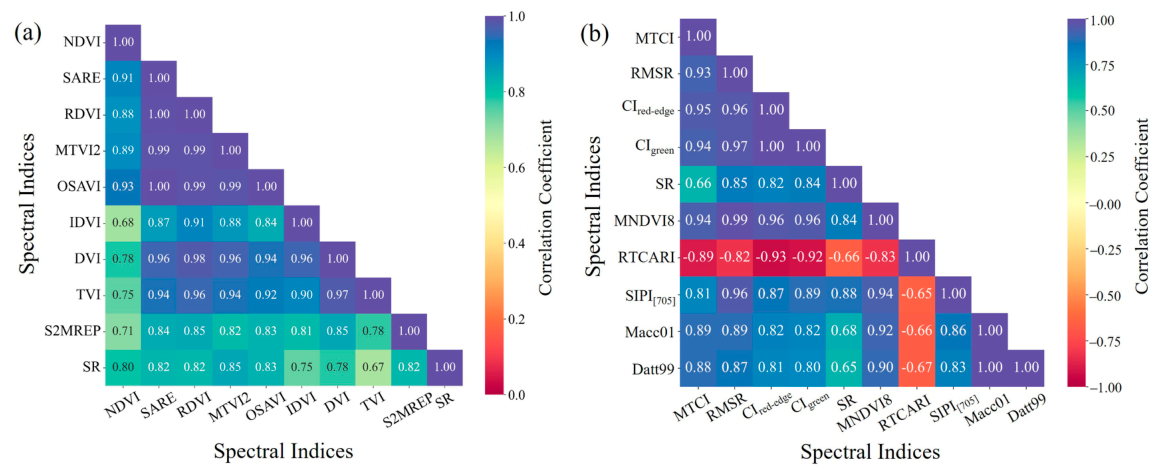
Figure 1. Inter-index correlation heatmaps for collinearity diagnostics of candidate vegetation indices: (a) indices related to LAI; (b) indices related to CCC.
Preprints 226579 g001
Figure 2. Feature importance ranking of LAI-related vegetation indices using random forest. Top: individual importance scores for each index. Bottom: cumulative importance distribution across ranked features.
Preprints 226579 g002
Figure 3. Feature importance ranking of CCC-related vegetation indices using random forest. Top: individual importance scores for each index. Bottom: cumulative importance distribution across ranked features.
Preprints 226579 g003
Figure 4. Architecture of the proposed dual-branch CNN–Transformer model for winter wheat LAI and CCC retrieval.
Preprints 226579 g004
Figure 5. Architecture of the proposed CNN–Transformer model and comparative baseline networks for ablation analysis.
Preprints 226579 g005
Figure 6. Schematic diagram of the unified progressive transfer learning strategy.
Preprints 226579 g006
Figure 7. Residual error distributions of candidate architectures (Models A–D) under different datasets and transfer learning strategies for winter wheat LAI and CCC retrieval.
Preprints 226579 g007
Figure 8. Split violin plots of winter wheat LAI and CCC retrieval residuals, comparing performance with versus without TL across different architectures, datasets, and observation platforms.
Preprints 226579 g008
Figure 9. Scatter plots of measured versus predicted winter wheat LAI using the optimal Model C under different training strategies and datasets. The red solid line represents the regression fit, and the gray dashed line is the 1:1 line. (Top row: Dataset I; Bottom row: Dataset II).
Preprints 226579 g009
Figure 10. Scatter plots of measured versus predicted winter wheat CCC using the optimal Model C. (Layout same as Figure 9).
Preprints 226579 g010
Figure 11. Split violin plots of winter wheat LAI and CCC retrieval residuals, comparing the impacts of Dataset I versus Dataset II across different architectures, training strategies, and observation platforms.
Preprints 226579 g011
Figure 12. Global SHAP feature importance summary plots for the proposed model evaluated on the UAV dataset under different pre-training strategies.
Preprints 226579 g012
Figure 13. Spatial distribution maps of winter wheat LAI and CCC retrieved from UAV hyperspectral imagery using the proposed CNN–Transformer transfer learning framework.
Preprints 226579 g013
Figure 14. RMSE comparison of winter wheat LAI and CCC retrievals across different model architectures (A–D), pre-training datasets, and transfer learning strategies at both ground (a, c) and UAV (b, d) observation scales.
Preprints 226579 g014
Figure 15. Global SHAP feature importance summary plots for the proposed model (Model C) evaluated on the ground dataset under different pre-training strategies.
Preprints 226579 g015
Table 1. Overview of winter wheat field and UAV experiments.
Year Number of Plots Nitrogen Levels Fertilization Treatments Irrigation Schemes Observation Type Measurement Period
2002 48 N1–N4 Uniform I1–I4 Ground-based 04/02 ~05/17
2004 42 Uniform Uniform Uniform Ground-based 04/14 ~ 05/19
2019 32 N1–N4 F1–F4 Uniform Ground-based 04/22 ~ 05/13
2021 32 N1–N4 F1–F4 Uniform Ground/UAV-based 04/14 ~ 05/18
Table 2. Statistical summary of field-measured LAI (m2 m−2) and CCC (μg cm−2) of winter wheat at different experimental years.
Year Parameter Number Minimum Maximum Mean Standard Deviation
2002 LAI 186 1.09 4.86 2.78 0.72
CCC 186 45.42 237.57 137.18 48.52
2004 LAI 85 1.35 5.20 3.12 0.85
CCC 85 73.77 296.91 167.36 47.99
2019 LAI 96 0.59 3.80 1.82 0.81
CCC 96 15.82 260.14 114.32 61.49
2021 LAI 63 0.16 4.07 2.00 0.94
CCC 63 2.90 241.45 122.43 61.27
Table 3. Input parameters and settings for the PROSAIL-D simulations.
Category Parameter Symbol Unit Range
Leaf level parameters Leaf structure index N - 1, 1.5, 2
Leaf chlorophyll content LCC μg cm−2 10~80; interval, 10
Leaf dry matter content Cm g cm−2 0.003, 0.004,0.005, 0.006
Leaf brown pigment content Cb - 0
Equivalent water thickness Cw cm 0.02
Leaf carotenoid content Car μg cm−2 25% LCC
Leaf anthocyanin content CAnt μg cm−2 2
Canopy level parameters Leaf area index LAI m2 m−2 0.5, 1, 2, 3, 4, 5, 6, 7, 8
Factor of dry soil Fsoil - 0.1, 0.25, 0.5, 0.75, 1
Average leaf angle ALA Degrees 26.8, 45, 45, 45, 57.3, 63.2
Hot spot parameter hotS m1 m−1 0.05
Fraction of diffuse incoming
Solar radiation
skyl - 0.5
Observation geometry Solar zenith angle θs Degrees 0, 10, 20, 30, 40, 50, 60
View zenith angle θv Degrees 0
Sun-sensor azimuth angle φ Degrees 0
Optimized parameters
(for Section 2.3.2)
Adjusted Average Leaf Angle ALAadj Degrees 62
Table 4. Vegetation indices used in this study.
Target VIs Formulation Reference
LAI NDVI ( R 800 R 670 ) / ( R 800 + R 670 ) [35]
DVI R 800 R 670 [36]
RDVI ( R 800 R 670 ) / ( R 800 + R 670 ) [37]
MTVI2 1.5 [ 1.2 R 800 R 550 2.5 R 670 R 550 ] ( 2 R 800 + 1 ) 2 ( 6 R 800 5 670 0.5 [38]
OSAVI ( 1 + 0.16 ) ( R 800 R 670 ) / ( R 800 + R 670 + 0.16 ) [39]
IDVI [ 1 + R 800 R 670 ] / [ ( 1 R 800 + R 670 ] [40]
SARE 1.25 ( R 800 R 670 ) / ( R 800 + R 670 + 0.25 ) [41]
TVI 0.5 [ 120 R 750 R 550 200 R 670 R 550 ] [42]
S2MREP 696 + 35 [ R 800 + R 670 / 2 R 700 ( R 740 R 700 ) ] + 38 R 740 [12]
SR R 800 / R 670 [43]
CCC MTCI ( R 754 R 709 ) / ( R 709 + R 681 ) [44]
RMSR ( R 750 / R 670 ) / ( R 800 + R 670 ) [45]
CIred-edge R 780 / R 705 1 [46]
CIgreen R 780 / R 550 1 [47]
SR R 800 / R 670 [43]
MNDVI8 ( R 755 R 730 ) / ( R 755 + R 730 ) [48]
RTCARI 3 ( ( R 750 R 705 ) 0.2 ( R 750 R 550 ) ( R 750 / R 705 ) [45]
SIPI [705] ( R 800 R 455 ) / ( R 800 + R 705 ) [49]
Macc01 ( R 780 R 710 ) / ( R 780 R 680 ) [50]
Datt99 ( R 780 R 710 ) / ( R 780 R 680 ) [51]
Table 5. Final selection of vegetation indices for LAI and CCC modeling.
Target Variable Selected VIs Target Variable Selected VIs
LAI DVI CCC MNDVI8
IDVI SIPI [705]
MTVI2 MTCI
RDVI RMSR
SARE CIgreen
Table 6. Comprehensive comparison of winter wheat LAI and CCC retrieval accuracy across different models and datasets.
Dataset Model Strategy LAI (m2 m−2) CCC (μg cm−2)
Ground UAV Ground UAV
R2 RMSE R2 RMSE R2 RMSE R2 RMSE
A Without TL 0.22 1.74 0.18 4.02 0.50 250.21 0.57 239.01
With TL 0.33 0.77 0.17 0.92 0.51 55.22 0.54 125.72
B Without TL 0.16 1.97 0.20 3.03 0.51 291.44 0.50 235.75
With TL 0.36 0.75 0.16 0.90 0.50 46.72 0.49 111.27
C Without TL 0.14 2.63 0.34 1.65 0.48 111.58 0.38 75.41
With TL 0.50 0.67 0.51 0.64 0.53 41.05 0.47 50.24
D Without TL 0.12 2.43 0.22 1.61 0.58 223.24 0.45 120.20
With TL 0.52 0.67 0.46 0.71 0.59 43.64 0.41 78.75
A Without TL 0.16 1.20 0.53 1.36 0.57 130.32 0.54 103.40
With TL 0.38 0.73 0.55 0.73 0.53 48.79 0.50 63.66
B Without TL 0.10 1.14 0.36 1.60 0.54 74.48 0.54 162.43
With TL 0.39 0.72 0.36 0.83 0.54 47.84 0.56 56.49
C Without TL 0.51 0.72 0.45 1.12 0.61 39.54 0.44 72.30
With TL 0.55 0.63 0.53 0.62 0.59 36.12 0.59 37.56
D Without TL 0.43 0.73 0.47 1.77 0.58 125.06 0.54 93.38
With TL 0.49 0.69 0.50 0.65 0.53 43.99 0.49 50.41
Disclaimer/Publisher’s Note: The statements, opinions and data contained in all publications are solely those of the individual author(s) and contributor(s) and not of MDPI and/or the editor(s). MDPI and/or the editor(s) disclaim responsibility for any injury to people or property resulting from any ideas, methods, instructions or products referred to in the content.
Copyright: This open access article is published under a Creative Commons CC BY 4.0 license, which permit the free download, distribution, and reuse, provided that the author and preprint are cited in any reuse.