

Submitted:
03 August 2026
Posted:
05 August 2026
You are already at the latest version
Abstract
Accurate atomic data for heavy ions are required for spectroscopic diagnostics and impurity transport modeling in magnetic-confinement fusion devices, particularly for tungsten and its neutron-induced transmutation products. In the present work, we investigate the ytterbium-like ions Ta IV, W V, Re VI, Os VII, Ir VIII, and Pt IX using complementary pseudo-relativistic Hartree–Fock (HFR) and fully relativistic multiconfiguration Dirac–Hartree–Fock (MCDHF) approaches. Semi-empirical calculations were first performed using the HFR method including core polarization corrections (HFR+CPOL). The evolution of correlation effects along the isoelectronic sequence was then analyzed through an alternative HFR(CV) model in which the most important core-excited configurations were introduced explicitly to account for core–valence interactions. Extensive least-squares fits to the available experimental energy levels were carried out for all ions considered. The results reveal that the HFR+CPOL approach provides an adequate description of Ta IV and W V, while explicit treatment of core–valence correlations becomes increasingly important from Re VI onwards owing to the growing interaction between the 5d5f and 5p55d3 configurations. New energy level classifications, level compositions, oscillator strengths, and transition probabilities are reported and critically assessed through comparisons between HFR and MCDHF calculations. The resulting dataset extends previous investigations of rhenium and osmium ions and provides benchmark atomic data for heavy-ion spectroscopy and future fusion-plasma applications.
Keywords:
atomic structure
; transition probabilities
; fusion plasma diagnostics
; tungsten transmutation products
; Yb I isoelectronic sequence
1. Introduction
The realization of fusion energy as a sustainable and large-scale energy source relies on the successful operation of magnetic-confinement devices such as ITER and, ultimately, DEMO-class reactors. In these systems, the interaction between the high-temperature plasma and plasma-facing materials plays a crucial role in determining both plasma performance and component lifetime. Spectroscopic diagnostics are among the most important tools available for monitoring plasma conditions, impurity transport, and radiative power losses, creating a continuous need for accurate atomic data for heavy ions.
Tungsten has been selected as the reference material for the ITER divertor because of its exceptional thermo-mechanical properties, including its high melting point, low sputtering yield, good thermal conductivity, and low tritium retention [1,2,3]. The adoption of a full tungsten divertor represents a major milestone in the design of ITER. However, tungsten atoms released from plasma-facing components through sputtering or erosion processes become ionized in the plasma and can generate substantial radiative losses due to their complex electronic structure and the very large number of transitions arising from their open-shell configurations. Consequently, reliable atomic data for tungsten ions are essential for plasma diagnostics, impurity transport studies, and radiation modeling in present and future fusion devices.
An additional challenge originates from neutron-induced transmutation processes occurring in tungsten under the intense 14-MeV neutron flux generated by fusion reactions. Detailed inventory calculations performed by Gilbert and Sublet [4] have shown that neutron-capture and subsequent decay processes progressively convert tungsten into neighboring heavy elements, primarily rhenium and osmium, while smaller but significant amounts of tantalum, iridium, and platinum are also produced. Depending on the irradiation conditions and operating lifetime, the concentration of these transmutation products may reach several atomic percent, leading to measurable modifications of the physical and mechanical properties of tungsten-based plasma-facing materials. Since these elements can subsequently enter the plasma through erosion mechanisms, their ionic spectra may contribute to the observed emission from fusion plasmas. Accurate atomic data are therefore required not only for tungsten ions themselves but also for the ions of the neighboring transmutation products.
The production of such data has motivated a series of recent investigations by our group. Extensive calculations of energy levels and radiative parameters were reported for Re III–V ions [5], while new datasets for osmium ions were published for Os V [6] and Os VI [7]. These studies highlighted the importance of relativistic and electron-correlation effects in heavy open-shell systems and provided data of direct relevance for spectroscopic diagnostics and plasma modeling. The present work constitutes a natural extension of these efforts toward the ytterbium-like sequence.
Among the transmutation products of tungsten, the Yb-like ions Ta IV, W V, Re VI, Os VII, Ir VIII, and Pt IX form a particularly interesting isoelectronic sequence. Their electronic structure is governed by the interplay between strong relativistic effects, extensive configuration interaction, and significant core-valence correlations. Previous experimental and theoretical studies have revealed substantial level mixing and complex coupling schemes in these ions, making accurate calculations particularly challenging. At the same time, the available spectroscopic information remains incomplete and heterogeneous along the sequence, especially for highly excited configurations and radiative transition probabilities.
In the present work, we perform a systematic investigation of the Yb-like ions Ta IV, W V, Re VI, Os VII, Ir VIII, and Pt IX using complementary pseudo-relativistic Hartree–Fock and fully relativistic multiconfiguration Dirac–Hartree–Fock approaches. Particular attention is devoted to the treatment of correlation effects and to the evolution of the atomic structure along the isoelectronic sequence. The resulting energy levels and radiative parameters provide new benchmark data for heavy-ion spectroscopy and are expected to contribute to future fusion-plasma diagnostics and modeling efforts.
2. Available Atomic Data
2.1. Tantalum (Z=73)
In 1978, Meijer and Metsch [8] found all the 14 levels of the 5d2 + 5d6s + 6s2 low-lying even configurations and all the 16 levels of the 5d6p and 6s6p odd configurations. In their work, they classified 114 lines in the 763.140-3076.058 Å region by using a Hilger and Watts E1 quartz prism spectrograph, the 6.65 m normal incidence vacuum spectrograph and the 6.6 m grazing incidence spectrograph of the Zeeman Laboratory. They also carried out pseudo-empirical calculations by fitting the Slater parameters and by introducing the observed energy levels in the Hartree-Fock method where the observed configurations (5d2 + 5d6s + 6s2 + 5d6p + 6s6p) were considered in the configuration interaction (CI) model. The fit reached a mean deviation (between the computed and observed energy levels) of 71 cm−1 and 160 cm−1 for the even and odd parities, respectively.
Eighteen years later, Kildiyarova [9] observed 16 of the 20 levels in the 5d5f odd configuration which gives strong transitions to the 5d2 levels. They classified 49 lines in the 555.124-648.656 Å spectral range using a triggered spark and a sliding spark source to excite the Ta IV spectrum and a 3-m normal incidence spectrograph with a reciprocal dispersion of 1.3858 cm−1 to photograph it. They performed a least-squares fitting calculation by including many more configurations in the odd CI model than the previous study, namely 5dnp (n=6,7) + 5dnf (n=5,6) + 6s6p + 6s5f + 5p55d3 reaching a mean deviation of 145 cm−1. By plotting the average energy of the configurations introduced in the model from Ta IV to Pt IX, they conclude on strong configuration interaction (CI) between the 5d5f and 5d7p odd configurations in Ta IV, between the 5d5f and 6s6p in Re VI and Os VII and the 5p55d3 open-core configuration crossed the 5d7p and 6s6p odd configurations along the Yb-like isoelectronic sequence resulting in important CI. In the same year, Churilov [10] measured all the 12 levels of the 5d7p configuration, three of the four missing levels of the 5d5f configuration and classified 66 lines in the 551.422-932.187 Å region using a 3 m normal incidence spectrograph with a plate factor of 1.38 Å in the first order, a sliding spark and a triggered spark light source for exciting the spectrum. They considered one more configuration, 5d7f, in the least-squares fit procedure for the odd parity giving rise to a mean deviation of 126 cm−1.
2.2. Tungsten (Z=74)
Yoca [11] have already carried out semi-empirical and ab initio atomic structure calculations in W V with the HFR approach, the Flexible Atomic Code (FAC) and the MCDHF method. Their work was based on the compilation of the spectroscopic data for Yb-like tungsten in NIST [12] which has collected energy levels and transitions obtained by Meijer [13] who observed the W V spectrum in the 63–219 nm wavelength range by using a sliding-spark light source and also by Kildiyarova [9] and by Churilov [10] who extended the identifications to the region 39–57 nm using similar light sources. There were 193 lines from 391.566 to 2187.270 Å and 59 experimental energy levels belonging to the 5d2, 5d6s, 5d6p, 6s6p, 5d5f and 5d7p configurations. Two levels of the 5d5f configuration are still missing with J=0 and J=6. The physical model considered in their HFR+CPOL calculations contained 45 configurations which describe a large part of the configuration interactions (CI). They compared to another HFR model (without the CPOL corrections), referenced to as HFR(CV), which contains 28 configurations among which some configurations had an open core subshell in order to take into account the core-valence interactions explicitly. In both models, they carried out a fitting procedure giving rise to a standard deviation of 20 cm−1, 132 cm−1 for the even and odd parities, respectively, for the HFR+CPOL model and 20 cm−1, 135 cm−1 for the even and odd parities, respectively, for the HFR(CV) model. They found a good agreement between the oscillator strengths computed by both these models meaning that the correlation effects with the core taken explicitly into account with the HFR(CV) model were well described by the HFR+CPOL model. They compared all methods used in their work and also with the RMBPT calculations made by Safronova [14] and they found an overall better agreement between the HFR+CPOL method and the FAC method where the uncertainty of the results was estimated at 15-20%.
2.3. Rhenium (Z=75)
Sugar [15] measured the spectra of Re VI using sliding-spark and triggered-spark discharges. These spectra were recorded photographically with the 10.7-m grazing-incidence and normal-incidence spectrographs and the 3-m normal incidence spectrograph. They observed 13 levels of the 5d2, 5d6s even configurations and 29 levels belonging to the 5d6p, 6s6p and 5d5f odd configurations where one of the four levels of the 6s6p configuration and 16 of the 20 levels of the 5d5f configuration were identified. By first performing HFR calculations with the least-squares adjustment of the energy parameters, this enabled them to identify 112 lines between 332.044 and 1513.957 Å. They introduced in their model a limited number of configurations, namely 5d2 + 5d6s + 6s2 and 5d6p + 6s6p + 5d5f for the even and odd parities, respectively. The fit provided a mean deviation of 64 cm−1 and 490 cm−1 for the even and odd parities, respectively. They tried to improve the fit by considering more CI with the introduction of the 5d7p and 4f135d3 odd configurations but they did not give the mean deviation value for the improved fit. It highlights nevertheless the importance of considering this core-excited configuration explicitly in the model to describe the significant core-valence correlations. The large sigma-value of the odd parity came from the difficulty of fitting the 5d5f odd configuration due to the collapse of the 5f orbital.
2.4. Osmium (Z=76) and Iridium (Z=77)
Van het Hof [16] identified 77 (5d2+5d6s)-5d6p lines in Os VII and 71 lines in Ir VIII between 13 even levels and 12 odd levels for both ions. The wavelengths of the transitions obtained by excitations in a triggered spark discharge and photographed on the 3 m normal incidence spectrograph at St. Francis Xavier University, range from 391.771 to 1319.811 Å for Os VII and from 337.535 to 1172.084 Å for Ir VIII. The 5d2-5d6p arrays were measured stronger than the 5d6s-5d6p arrays in both ions. After completing the fit procedure, the standard deviations between the calculated and the observed energy levels were found to be 114 cm−1 and 354 cm−1 for the even and odd parities, respectively, in Os VII, and 124 cm−1 and 336 cm−1 for the even and odd parities, respectively, in Ir VIII.
The 72 and 58 weaker (5d2+5d6s)-5d5f lines in Os VII and in Ir VIII were identified by Kildiyarova [17] in the 288.274-537.010 Å region and in the 237.098-292.817 Å region, respectively, as well as 18 of the 20 levels of the 5d5f configuration. They introduced 7 configurations in their HFR odd model, namely 5dnp (n=6,7) + 6s6p + 5dnf (n=5,6,7) + 5p55d3 and the fit reached a mean deviation of 204 cm−1 and 226 cm−1 for Os VII and Ir VIII, respectively. From their semi-empirical HFR calculations, the odd level composition presented an important mixture between the 5d5f and 6s6p odd configurations as well as between the 5d5f and the 5p55d3 odd configurations where for a few energy levels, the dominant spectroscopic term in the level composition belongs to the 5p55d3 core-excited configuration. For example, the principal component of the level measured at 388 229 cm−1 (J=2) in Ir VIII appeared as 5p55d35S with 19%. This underlines the importance of including this configuration explicitly in the model in order to take into account all major CI.
2.5. Platinum (Z=78)
Kildiyarova [18] photographed the spectrum of Pt IX using a 2-m and a 10-m grazing incidence spectrographs where the source used in laboratories was a triggered spark. This enabled them to measure 9 levels of the 5d2 even configurations, 12 levels of the 5d6p and 18 of the 20 levels of the 5d5f odd configurations. They were able to predict the 106 observed lines belonging to the 5d2-5d(6p + 5f) transition arrays between 216.575 and 345.804 Å thanks to the HFR calculations and a least squares fit. The 5d6s-5d6p transitions were not studied because there were not intense hot spectra at > 350 Å. The configuration interaction model introduced in the calculations was 5d2 + 5d6s + 6s2 and 5dnp (n=6,7) + 5dnf (n=5,6,7) + 6s6p + 5f6s + 5p55d3 for the even and odd parities, respectively. After the fit, the agreement between the experimental and the calculated level values for both even and odd parity systems was qualified to be quite good in a view of the standard deviation of 62 cm−1 and 324 cm−1 for the even and odd parities, respectively. From the computed level compositions, they concluded that there was even more mixing between the 5d5f and 5p55d3 odd configurations than in Os VII and Ir VIII and the jj coupling representation seemed to be more adequate than the LS designation especially for the 5d5f levels even though both designations showed important mixing.
Azarov and Churilov [19] extended the observed spectrum from 327.777 to 1055.171 Å corresponding to the (5d2 + 5d6s)-5d6p transitions thanks to high-resolution VUV spectrographs. The spectrum was excited in a plasma by a three-electrode low-inductance vacuum spark, the operating discharge voltage being 4.0–4.5 kV. They identified 4 more levels belonging to the 5d6s even configuration and classified 26 transitions where one of which, observed at 327.777 Å in [19] had already measured by Kildiyarova [18] at 327.574 Å. They also computed the transition probabilities, , by performing HFR calculations and a fit procedure with a method based on the orthogonal operators. The fit enabled to achieve a mean deviation of 30 cm−1 and 33 cm−1 for the even and odd parities, respectively, optimizing only the levels observed in their work belonging to the 5d2, 5d6s and 5d6p configurations.
2.6. Other Studies on Ytterbium-like Ions of Interest
Azarov [20] performed semi-empirical calculations using the orthogonal operators on the 5d2, 5d6s and 5d6p configurations for all Yb-like ions from Ta IV to Hg XI. He obtained an agreement between the observed levels and the eigenvalues 5 times and 10 times better than the previous least-squares calculations with the Slater parameters for the even and odd systems, respectively. This made it possible to predict the energy of unknown levels, to supply a set of fitted parameters and to evaluate the evolution of these parameters and their effects along the isoelectronic sequence. This evolution was extrapolated to obtain the parameters for the Hg XI ions in order to verify the position of the observed energy levels. These results will also be useful for the ions of the neighboring sequences that have the 5d3 and 5d4 ground-state configurations.
Another previous study on the computations of excitation energies and transition rates in Yb-like ions (Z = 72 - 100) using the Relativistic Many-Body Perturbation Theory (RMBPT) was carried out by Safronova [21]. They considered a model composed of the 5d2, 5d6s, 6s2 and the 5d6p, 5d5f and 6s6p even and odd configurations, respectively. The observed levels and the levels computed with their RMBPT method were listed for Re VI to Hg XI and only the E1 line strengths in length and velocity gauges for Re VI were tabulated. They well reproduced the low-lying observed energy levels but there was a disagreement with the highly excited levels (2 000 - 10 000 cm−1) belonging to the 5d5f configurations especially due to important mixing between the 5d5f configuration and the 5p55d3 core-excited configuration. They also mentioned that neither nor coupling describes physical states properly.
3. Numerical Methods
3.1. The Pseudo-Relativistic-Hartree-Fock (HFR) Calculations with the Core Polarization Corrections (CPOL)
The first computational approach used in this work was the pseudo-relativistic Hartree–Fock (HFR) method, originally developed by Cowan [22] in order to iteratively solve the Hartree-Fock equations which are obtained by a variational principle minimizing the average energy of each non-relativistic electronic configuration introduced in our model. The resulting Atomic State Functions of parity P, total angular momentum J with projection were expanded in terms of Configuration State Functions in coupling: where define each CSFr uniquely and are the mixing coefficients obtained by the so-called Self-Consistent-Field method. It is meaningful to consider the Coulomb correlation effects between electrons in the calculations of the wave function. Migdalek and Baylis [23] have suggested to describe the intravalence correlations by introducing explicitly in the calculations a large (but finite due to limited resources) number of valence configurations while the correlations with the core were described by a core polarization model potential. The method was thus modified by the Atomic physics and Astrophysics unit by introducing the polarization effects of the ionic core in the HFR method as described in [24,25] in order to take all correlation effects into account. This method is referred to as HFR+CPOL. In order to reproduce as well as possible the energy level structure, the physical HFR+CPOL model was based on the previous work in W V [11] since it had been confirmed by the very good agreement obtained between the HFR+CPOL method and two other atomic structure calculation methods, namely the Flexible Atomic Code (FAC) and the Multiconfiguration Dirac–Hartree-Fock (MCDHF) method.
Therefore, for all ions in the ytterbium isoelectronic sequence studied in this work, we have decided to introduce explicitly in the computations the same set of configurations namely 22 even configurations, 5d2 + 6sns (n=6-7) + 5dns (n=6-7) +5dnd (n=6-7) + 6snd (n=6-7) + 6pnp (n=6-7) + 6pnf (n=5-7)+ 6dnd (n=6-7) + 6d7s + 7s2 + 7p2 + 7s7d + 7pnf (n=5-7), and 21 odd configurations, 5dnp (n=6-7) + 6snp (n=6-7) + 5dnf (n=5-7) + 6snf (n=5-7) + 6pnd (n=6-7)+ 6p7s + 6dnf (n=5-7) + 7snf (n=5-7) + 7s7p + 7p7d. The pseudo-potential which describes the core polarization effects depends on two parameters, the ionic-core radius (rc) and the static dipole polarizability () of the ionic core. These parameters were evaluated for all the six Yb-like ions studied in this work by considering the same Yb III-type ionic core with 68 electrons surrounded by two valence electrons as already considered in the previous study on W V [11]. The rc-value was estimated by the mean value of the outermost orbital of the ionic core computed in the HFR method, namely , and the -value was obtained by an extrapolation of the known -values taken in [26] along the erbium isoelectronic sequence as given in the Figure 1. This figure represents first the evolution of the rc-values along the isoelectronic sequence in green and also the extrapolation of the -values where the values that were already known in [26] were represented with a full black circle and the extrapolated values were shown with an empty blue circle. Note that the -value for W(74) had already been extrapolated and was taken from [11].
Because we cannot introduce an infinite number of configurations in the calculations and describe all configuration interactions, we have introduced a scaled factor of 0.85 which reduced all the Slater integrals of the Hamiltonian and thus modified the mixing coefficients in order to include the effects of far away interacting configurations [22]. Then, for all elements studied in this work, we performed a least-squares adjustment of the computed energy levels by introducing the observed energy levels in our calculations. It allowed to reproduce more accurately the level structure and to compute the radiative parameters with more precision by optimizing the radial parameters of the Hamiltonian such as the average energies (), the Slater integrals (, and ), the spin-orbit parameters (), as well as the effective interaction radial parameters and that represent weak CI effects on configurations with equivalent electrons in p and/or d orbitals.
The number of fitted levels, i.e., observed levels, and the standard deviation of the fit are given in the Table 1. The additional energy levels observed in each parity of Ta IV but not observed in W V were the 6s21S0 even level and the 5d5f 3P0o odd level. For all ions studied in this work, the radial parameters of the 5d2, 5d6s, 5d6p, and 5d5f configurations were adjusted semi-empirically. The average energy of the 6s2 even configuration had been fitted only for Ta IV. All radial parameters of the 5d7p, 6s6p configurations have been fitted only for Ta IV and W V and only the average energy of the 6s6p configuration had been fitted for Re VI up to Ir VIII.
For Ta IV, we obtained a better agreement between the observed and the computed energy levels with the HFR+CPOL method for the even and odd parities than Meijer and Metsch [8] had previously achieved. The standard deviation in our work was found to be 22 cm−1 and 106 cm−1 for the even and odd parities, respectively, while Meijer and Metsch [8] obtained a deviation slightly higher, 70 cm−1 and 160 cm−1 for the even and odd parities, respectively. Then, Kildiyarova [9] and Churilov [10] improved the deviation for the odd parities by introducing more odd configurations and they obtained 145 cm−1 and 126 cm−1, respectively, which is still higher than the deviation obtained in this work. The reason for our better fit could be the CPOL effects that we considered through the pseudo-potential model and also the introduction of more significant CI in the HFR method which allowed us to reproduce more accurately the observed energy level structure.
As already mentioned, the configuration model used in the HFR+CPOL method was based on Yoca [11] who also performed a semi-empirical calculation giving rise to a standard deviation of 20 cm−1 and 132 cm−1 for the even and odd parities in W V, respectively. In this work, we tried to reproduce the same fitting procedure and we obtained nearly the same value of the deviation namely 26 cm−1 and 123 cm−1 for the even and odd parities, respectively. Moreover, we compared the transition probabilities computed in the previous work with our study and we observed a very good agreement between both calculations namely the mean ratio =1.02 ± 0.14 where "0.14" stands for the standard deviation of the ratio.
For all ions after W V along the sequence, namely for Re VI, Os VII, Ir VIII and Pt IX, the fit became increasingly difficult, especially for the odd parity, as reflected by the increasing of the standard deviation of the fit for the odd parity in Table 1. For example, the standard deviation of the odd parity in Re VI was equal to 347 cm−1 which is more 2.5 times higher than the one of the odd parity of W V.
The first reason for the higher standard deviation is that there is only one level of the 4 levels of the 6s6p configurations that have been identified in Re VI and none in the following ions which restricted the number of fitted parameters related to the 6s6p configurations. Moreover, no levels belonging to the 5d7p configurations were identified until now for all ions after W V in the Yb isoelectronic sequence, namely Re VI, Os VII, Ir VIII and Pt IX, which limited the global adjustment of the semi-empirical computed energy level structure for these four ions studied in this work. Indeed, some previous works on these ions have already presented a high deviation in the least-squares adjustment meaning that the energy level structure is complex in these ions. In Re VI, Sugar [15] found a mean deviation of 64 cm−1 and 490 cm−1 for the even and odd parities, respectively, which are slightly higher than the ones obtained with our HFR+CPOL method certainly because of the CPOL effects introduced in the HFR method as well as the fit of the Rk parameters in our calculations that were kept fixed in Sugar [15]. This allowed us to obtain a better mean deviation. Van het Hof [16] obtained a deviation of 114 cm−1 and 354 cm−1 for the even and odd parities, respectively, in Os VII and 124 cm−1 and 336 cm−1 for the even and odd parities, respectively, in Ir VIII. Kildiyarova [17] improved the agreement between the observed and the computed odd energy levels by introducing more configuration interactions in their model reaching a deviation of 204 cm−1 and 226 cm−1 for the odd parity of Os VII and Ir VIII, respectively. In Pt IX, Kildiyarova [18] performed a fit reaching 62 cm−1 and 324 cm−1 for the even and odd parities, respectively. Azarov and Churilov [19] obtained a much smaller deviation, 30 cm−1 and 33 cm−1, for the even and odd parities, respectively, because the fit was carried out only on the 5d2, 5d6s and 5d6p configurations while in Kildiyarova [18] the 5d5f configuration was also fitted. It showed that the fit of the 5d5f configuration gave some problems as already noticed in Sugar [15] for Re VI because of the contraction of the 5f orbital along the Yb isoelectronic sequence. For Os VII, Ir VIII and Pt IX, the authors of the previous studies obtained a better fit than with our HFR+CPOL method because of the increasing interactions between the observed configurations and especially the 5p55d3 open-core configuration that were introduced explicitly in the model of Kildiyarova [17] and Kildiyarova [18] but not in our HFR+CPOL model where the core correlation effects were considered by a corrective pseudo-potential. Sugar [15] also suggested to introduce the 4f135d3 core-excited configuration in the model to improve the fit.
Another important reason which could explain why we obtained a high value of the standard deviation for Re VI up to Pt IX with the HFR+CPOL model is that the CPOL corrections could no longer be valid for these ions. Indeed, we considered valence-valence interactions through the configuration interactions by including explicitly in the calculations a large number of valence configurations and the correlations with the core were taken into account through a pseudo-potential which was introducing as a correction to the Hamiltonian. This correction and thus the HFR+CPOL approach is only valid if the core-excited configurations do not overlap the configurations of interest namely if the interaction effects between them remain small. We can estimate the validity of the HFR+CPOL approach by plotting the average energies of the core-excited configurations with one electron excitation from the 5p and 4f core orbitals and the valence configurations of interest for all ions computed with the HFR method along the Yb isoelectronic sequence as represented in Figure 2. The black and blue colors represent the even and odd configurations of interest, respectively. The red and green colors stand for the core-excited configurations with one hole in the 4f and 5p core orbitals, respectively.
For Ta IV and W V, the lowest 5p55d26p, 5p55d3 and 5p55d26s open-core configurations are well above the configurations of interest. However, the 4f135d3 core-excited configuration is closer to the 5d7p and 5d5f odd configurations but the overlap and so the configuration interactions between the 4f135d3 core-excited configuration and the 5d7p and 5d5f configurations were not significant as we can see in the Figure 3. In this figure, the two red lines represent the overlap in energy of the 4f135d3 core-excited configuration with the two other configurations. The energy overlap was over an interval of nearly 10 800 cm−1 (≈ 6%) and 8 500 cm−1 (≈ 3%) for Ta IV and W V, respectively. Therefore, the correlation effects with the core can be described by the CPOL corrections at least for the ions Ta IV and W V.
For Re VI up to Pt IX, these correlation effects with the core can no longer be described by the CPOL corrections because the core-excited configurations become too close to the configurations of interest and the interactions with the core become thus too significant to be treated as a correction to the Hamiltonian. In general, we observe this situation when the ionization stage increases [7]. Therefore, we need to introduce these core-excited configurations explicitly in our HFR model and the correlation effects with the core as well as the valence-valence correlations are thus described by the configuration interactions. We should introduce an infinite number of core-excited configurations to have a complete calculation but we cannot treat all electronic correlations owing to the limited resources. We thus introduced only the most important and the most interacting core-excited and valence configurations explicitly in our calculations. In the HFR+CPOL method, the core correlation effects are described in a different way by considering the CPOL corrections where these effects are treated as a whole with a pseudo-potential and are introduced in the Hamiltonian as a perturbation.
In addition to the conventional representation, the Cowan code provides an alternative level classification in the so-called -coupling scheme. In this representation, each open subshell () is characterized by an angular momentum () obtained from the coupling (+→), and the resulting subshell angular momenta are coupled successively according to
Following Cowan [22], this ( …) representation may be regarded as a generalization of the usual -coupling scheme. It does not correspond to the fully relativistic coupling used in MCDHF calculations, but provides a convenient alternative classification of the intermediate-coupling eigenvectors. In the present work, both and Cowan compositions were analyzed in order to assess the coupling properties of the calculated levels.
3.2. The Pseudo-Relativistic-Hartree-Fock (HFR) Calculations with the HFR(CV) Model
Along the ionization stages of the Yb isoelectronic sequence from Re VI to Pt IX, the 5d55d3 configuration crossed over the configurations of interest strongly interacting especially with the 5d7p and 5d5f configurations as we observed in the Figure 2. This means that the configuration interactions between these configurations were important and the mixing between these configurations was increasingly significant in the semi-empirical energy level composition, as already noticed in previous studies [9,17,18]. For these ions, we instead performed HFR computations with a model that considered explicitly the core correlation effects through the configuration interactions. The second HFR model (referred to as HFR(CV)) was composed of the most interacting valence configurations to describe the intravalence correlations and the core-excited configurations with a single excitation from the 5s, 5p or 4f core orbitals that interact the most with the 5d2, 5d6s, 6s2, 5d6p, 6s6p, 5d5f and 5d7p configurations in order to describe explicitly the core-valence correlations. In other words, the Atomic State Function expansion was composed of 22 even configurations, 5d2 + 5d6s + 6s2 + 5d7s +5d6d + 5d7d + 6s7s + 6s6d + 6s7d + 6p2 + 6p7p + 6p5f + 5p55d26p + 5p56s26p + 5p55d6s6p + 5p55d25f + 5p55d27p + 5s5p65d3 + 5s5p65d26s + 5s5p65d6s2 + 4f135p65d26p + 4f135p65d6s6p, and 20 odd configurations, 5d6p + 6s6p + 5d7p + 5d5f + 5d6f + 5d7f + 6s7p + 6s5f + 6s6f + 6p6d + 6p7s + 5p55d3 + 5p55d26s + 5p55d6s2 + 5p55d6p2 + 5p56s6p2 + 5s5p65d26p + 5s5p65d6s6p + 4f135p65d3 + 4f135p65d26s.
We have used this HFR(CV) model not only for Re VI to Pt IX but also for Ta IV and W V in order to compare the transition probabilities obtained with the HFR(CV) model and those obtained with the HFR+CPOL method in the case of Ta IV and W V. A fitting procedure was also carried out with the HFR(CV) model where the standard deviations for all ions studied in this work are represented in Table 1. As we observed in this table, the fit of the even parity was not really improved because the inclusion core-excited configurations in the CI expansions increases the level mixing. In addition, when the atomic number increases, the level composition in the even parity becomes slightly more mixed as we can see in Table 2 where the mean purity of the observed levels obtained with the HFR(CV) model is shown in the and representation for Ta IV up to Pt IX. One can notice that the mean purities for Ta IV and W V were very close to the ones obtained with the HFR+CPOL method. The mean purity is given by the average value of the squares of the mixing coefficients of the dominant spectroscopic terms in the level compositions for all observed levels. This mixing could explain the slight increase of the mean deviation in the even parity along the sequence. However, the fit of the odd parity was significantly improved with the HFR(CV) model compared to the HFR+CPOL model especially for Re VI up to Pt IX. The fit became nevertheless more difficult for Ir VIII and Pt IX owing to the increasing mixing especially between the 5p55d3 and 5d5f configurations represented by a higher value of the standard deviation for both ions. Indeed, as shown in the Table 2 for Re VI up to Pt IX, the mixture of the or terms in the level composition increases along the sequence especially for the odd parity. This important mixture did not allow us to identify clearly one level in Ir VIII measured at 406 542 −1 () and two levels in Pt IX measured at 438 038 cm−1 () and 470 214 cm−1 () because of the large deviations from the HFR(CV) level energies (2 979 cm−1, 6 235 cm−1 and 7 838 cm−1, respectively). These levels have been thus removed from the fit and are listed with one star in Table 8 for Ir VIII and Table 9 for Pt IX. In general, we expect that when the ionic charge increases, the level structure becomes increasingly spread out represented by an increase in the energy gap between each configuration in each parity along the sequence which means that the level composition should present decreasing mixing. This is what we observed in Table 2 for the odd parity in Ta IV and in W V but in our study, it was nevertheless difficult to conclude that there were less and less mixing along the sequence because of the increasing interactions between each odd configuration and also between the core-excited configurations and the configurations of interest as showed in Figure 2.

Table 1.
Number of fitted levels and deviation obtained after the fit along the Yb isoelectronic sequence from Ta IV to Pt IX with the HFR+CPOL and HFR(CV) models.
Table 1.
Number of fitted levels and deviation obtained after the fit along the Yb isoelectronic sequence from Ta IV to Pt IX with the HFR+CPOL and HFR(CV) models.
| Even parity | Odd parity | |||||
|---|---|---|---|---|---|---|
| nbr of fitted levels | (cm−1) | (cm−1) | nbr of fitted levels | (cm−1) | (cm−1) | |
| Ta IV | 14 | 22 | 24 | 47 | 106 | 118 |
| W V | 13 | 26 | 31 | 46 | 123 | 141 |
| Re VI | 13 | 30 | 37 | 29 | 347 | 253 |
| Os VII | 13 | 31 | 40 | 30 | 779 | 139 |
| Ir VIII | 13 | 35 | 47 | 29 | 1216 | 571 |
| Pt IX | 13 | 38 | 53 | 28 | 3363 | 422 |
One can also see in Table 2 that the coupling is quite good for the even parity and the coupling seems to be more adequate to identify clearly the observed odd levels due to less mixing especially for the 5d5f levels but for the level designation in Pt IX neither the representation nor the representation is adequate because of the small value of the mean purity of the observed levels in both representations. Thus, some levels cannot be identified unambiguously, as discussed in [18,21]. In order to follow the same consistency as the previous studies in the Yb isoelectronic sequence and make better comparisons with future studies in this same sequence, we decided to identify all levels in coupling. The first two components in the composition of all levels fitted with the HFR+CPOL model as well as the HFR+CPOL energy values for Ta IV and W V are available in Table 4 and Table 5, respectively. The two first components in the composition in coupling of all levels fitted with the HFR(CV) model as well as the HFR(CV) energy values for Re VI, Os VII, Ir VIII and Pt IX are shown in Table 6, Table 7, Table 8 and Table 9. In these six energy tables, the first term in the compositions computed with the Cowan code [22] as well as with the MCDHF method [27] are also shown for better and easier future level comparisons using other methods that will be based on the coupling.
From these tables, we can clearly conclude that the coupling is quite good at least for the even parity as well as for the 5d6p and 6s6p odd configurations. The representation shows less mixing for the 5d7p and 5d5f odd configurations than the coupling except for Pt IX where both and representations give important mixing. In Table 4 and Table 5, the Ta IV and W V level compositions in the coupling show important mixing between the 5d5f and 5d7p odd configurations, as already discussed in [9]. In Ta IV, the first dominant term in the composition of the 5d7p and 5d5f levels can sometimes reach less than 30% for example the level measured at 180 137 cm−1 () presents an important mixture in coupling of 25% 5d7p (2D) 3D o + 23% 5d5f (2D) 1D o. In W V, the 5d5f and 5d7p configurations are still mixed but the mixing is slightly less important than in Ta IV as presented in Figure 2 where the average energy of these two configurations diverges. Kildiyarova [9,17] have already observed in their semi-empirical level compositions that the 5d5f and 6s6p odd configurations are mixed for Re VI, Os VII and Ir VIII. Indeed, Figure 2 confirms their computations because the average energy of the 5d5f and 6s6p odd configurations is getting closer to each other up to Re VI and then diverges along the Yb isoelectronic sequence giving rise to a swap of the positions of these two configurations after Re VI. For example, in Re VI, a level computed at 295 260 cm−1 () is composed of 44% 6s6p (2S) 1P o + 33% 5d5f (2D) 3D o. In Os VII, the two most important LS spectroscopic terms in the composition of the level measured at 356 849 cm−1 () are 61% 5d5f (2D) 3P o and 24% 6s6p (2S) 3P o. Kildiyarova [17,18] have also observed important mixing between the 5p55d3 and 5d5f odd configurations in Os VII, Ir VIII and Pt IX that is also confirmed by the Figure 2 where the average energy of the 5p55d3 core-excited configuration crossed the 5d5f as well as the 5d7p odd configurations along the sequence. Indeed, a level computed at 422 778 cm−1 () in Os VII is composed of 41% 5d7p (2D) 3D o + 15% 5p55d3 (2D) 3P o. In Ir VIII and Pt IX, the mixing between the 5p55d3 and 5d5f configurations is getting worse. Indeed, 5 and 8 levels present more than 15% of 5p55d3 in their composition for Ir VIII and Pt IX, respectively. It is even more interesting to note that one level in Ir VIII measured at 397 557 cm−1 () and one level in Pt IX observed at 424 403 cm−1 () have a dominant component of 36% 5p55d3 (4P) 5S o and of 21% 5p55d3 (4P) 5S o, respectively. However, the representation of these levels is 30% 5d5f (2D5/2) o and 27% 5d5f (2D3/2) o, respectively.
Table 2.
The mean purity of the observed levels obtained after the fit for all Yb-like ions studied in this work namely Ta IV - Pt IX with the HFR(CV) model in and coupling defined by Cowan [22]. The mean purity in coupling given by the MCDHF method is also shown.
Table 2.
The mean purity of the observed levels obtained after the fit for all Yb-like ions studied in this work namely Ta IV - Pt IX with the HFR(CV) model in and coupling defined by Cowan [22]. The mean purity in coupling given by the MCDHF method is also shown.
| Ta IV | W V | Re VI | |||||||
|---|---|---|---|---|---|---|---|---|---|
| Even | 0.91 | 0.89 | 0.81 | 0.89 | 0.89 | 0.84 | 0.86 | 0.87 | 0.84 |
| Odd | 0.61 | 0.76 | 0.74 | 0.67 | 0.87 | 0.81 | 0.62 | 0.80 | 0.78 |
| Os VII | Ir VIII | Pt IX | |||||||
| Even | 0.84 | 0.86 | 0.86 | 0.83 | 0.85 | 0.88 | 0.81 | 0.84 | 0.89 |
| Odd | 0.59 | 0.77 | 0.74 | 0.55 | 0.73 | 0.74 | 0.47 | 0.64 | 0.70 |
3.3. The Core Correlation Effects on the Transition Probabilities Computed with the HFR+CPOL and the HFR(CV) Models
After performing the fitting procedure for both HFR+CPOL and HFR(CV) models, we introduced the optimized values of the radial parameters in the calculations of the electric dipole (E1) transitions. The calculation accuracy of the transition probabilities () and the oscillator strengths () is thus improved with the least-squares fit of the level structure. For a comparison between a reference data set and a less reliable one, Kramida [28] suggested to plot the logarithm of the ratio of the transition probabilities computed by a less reliable method and a reference one as a function of the logarithm of the line strength. In order to estimate the effects of the core-valence (CV) correlation on the transition probabilities, we have carried out a series of HFR calculations along the sequence with the same CI expansions as in our HFR+CPOL model. The comparisons of the -values computed with the less reliable HFR and the reference HFR+CPOL methods, as represented in Figure 4 for Ta IV and Figure 5 for W V where only the transitions with log() > -4 were plotted, lead us to conclude that the HFR+CPOL method reduced the -values by nearly 20% on average, as expected [29]. The HFR method is the less accurate method because only intravalence interactions were taken into account. In both figures, the logarithm of the ratio of the weighted transition probabilities associated with the selected observed lines (221 among the 229 observed in Ta IV and 193 in W V) and computed by the HFR and HFR+CPOL methods, i.e., , was thus plotted as a function of the logarithm of the HFR+CPOL line strength, namely . The matrix element was more affected by the polarization effects which reduced it by about 35% and 40% in Ta IV and W V, respectively, due to the penetration of the 5f orbital into the ionic core.
Figure 4 and Figure 5 also show a very good agreement between the HFR+CPOL and HFR(CV) models for Ta IV and W V which means that the CPOL potential model describes in an equivalent way the core-valence correlations introduced explicitly in the HFR(CV) model. For the 221 and 193 lines measured in experiments for Ta IV [8,9] and W V [12], respectively, the mean ratio / = 1.08 ± 0.24 and 1.02 ± 0.36 for Ta IV and W V, respectively.
For Re VI up to Pt IX, we performed computations with the HFR(CV) model, instead of the HFR+CPOL model as already explained, for which we were able to estimate the effects of the CV correlations on the computed -values. From Figure 6 where all observed lines have a log()-value bigger than -4 for Re VI up to Ir VIII but where two transitions in Pt IX have a log()-value lower than -4, it is shown that the HFR(CV) -values are lower than the HFR -values by approximately 30%, 25%, 35% and 34% on average for Re VI, Os VII, Ir VIII and Pt IX, respectively. The CV effects are thus more important for Ir VIII and Pt IX as we can also see in Figure 6 where the clouds of points are more spread out. Indeed, as already shown previously in Figure 2, the configuration interactions between the core-excited configurations and the ones of interest become more significant for Ir VIII and Pt IX. This demonstrates the importance of including the CV correlations explicitly in our model.
3.4. The fully Relativistic Multiconfiguration Dirac-Hartree-Fock (MCDHF) Calculations
The second method called the fully Relativistic Multiconfiguration Dirac–Hartree–Fock (MCDHF) method [27], as implemented in the General Relativistic Atomic Structure Package (GRASP2018) [30], is used to estimate the accuracy of the results by comparing the transition probabilities obtained from the HFR+CPOL method for Ta IV and W V or from the HFR method with the HFR(CV) model for Re VI up to Pt IX and the MCDHF method which are two completely different approaches.
As described in [31], the Atomic State Functions (ASF) of parity P and total angular momentum J of projection M are expanded in terms of Configuration State Functions (CSF) in coupling: , where contains all information to define the CSF uniquely (i.e. the coupling scheme, the occupation number of orbitals, etc.) and are the mixing coefficients verifying the normalization condition: in which is the CSF number introduced in the model. Each CSF in the list is built from antisymmetrised products of one-electron relativistic spin orbitals. The list of CSFs was composed of multireference (MR) and correlation CSFs. The CSFs that strongly interact with the targeted CSFs were grouped together in the MR. The correlation CSFs that correct the reference CSFs were generated by using the active set (AS) approach which consists of allowing excitations of electrons from orbitals in the MR to the correlation orbitals in the AS.
Our calculations were the same for all ions along the Yb isoelectronic sequence studied in this work and began with an optimization of all orbitals (core and 5d valence orbitals) on the ground state (5d23F2) with the Optimal Level (OL) mode [27]. Then, we used the previously optimized radial parts in order to perform two different optimization schemes for each parity. For the even parity, only the 6s and 5d valence orbitals were optimized on all the 14 levels of the MR even configurations (5d2, 5d6s, 6s2) and the 6s, 6p, 7p, 5d and 5f valence orbitals were optimized on all the 47 levels of the MR odd configurations (5d6p, 6s6p, 5d5f, 5d7p) with the Extended Optimal Level (EOL) mode by freezing all the other orbitals already optimized in the previous calculation [27].
In the layer-by-layer (LBL) approach adopted in this study, the maximum values of the principal quantum number for each azimuthal quantum number l, l, are increased by steps until a convergence is reached by adding new correlation orbitals by layer in the list. In order to achieve this convergence, three steps of valence-valence correlations, referred to as VV1, VV2 and VV3, were considered where all the single and double (SD) excitations from the spectroscopic orbitals (5d, 6s for the even MR and 5d, 6s, 5f, 6p, 7p for the odd MR) to the orbitals in the active set were allowed. We carried out an Extended Optimal Level (EOL) optimization only for the radial parts of the last layer of orbitals in the AS that was not yet optimized in the previous calculations [30]. The orbitals that were already optimized were kept frozen. The first AS (VV1) was {7s,6p,6d,5f} and {7s,8p,6d,6f} for the even and odd parities, respectively. In the second layer of valence-valence correlations (VV2), we increased the list of CSFs by considering the AS {8s,7p,7d,6f} and {8s,9p,7d,7f} for the even and odd parities and finally the AS {9s,8p,8d,7f} and {9s,10p,8d,8f} for the even and odd parities, respectively, were considered in a last layer of valence-valence correlations (VV3) giving rise to 446 and 688 CSFs for the even and odd parities, respectively. We obtained the convergence of the results and a good agreement with the experimental level energies after the third optimization step as we can see in Table 3 for Ta IV. This table shows the average relative difference between the energy levels computed with the MCDHF method and the observed energy levels [8,9,10], (E-Eobs)/Eobs, and also the average relative difference between the energy levels computed in the ith and i-1th steps, (Ei-Ei−1)/Ei−1, for all calculation steps in Ta IV. The latter especially reached 0.06% and 0.01% for the even and odd parities, respectively, in the last optimization step (VV3) which justified stopping the increase of the AS at this stage.
For the core-valence (CV) and core-core (CC) calculations, we did not increase the AS and dit not reoptimize the orbitals. We considered the same AS and the radial parts optimized in the last VV calculation step, namely (VV3), to perform only a Relativistic Configuration Interaction (RCI) calculation where the QED effects were introduced in the Dirac-Coulomb-Breit Hamiltonian. For the CV correlations, we first allowed one hole in the 4f core orbital with single and restrictive double (SrD) excitations from the MR to the orbitals in the AS, referred to as CV(4f). Then, we considered one hole in the 4f or 5p core orbitals with also SrD excitations from the MR to the orbitals in the AS, referred to as CV(4f,5p). For the CC correlations, we allowed one hole in both 4f and 5p core orbitals and we considered SrD excitations from the MR to the orbitals in the AS, referred to as CV+CC(4f,5p). Then, we treated more CV correlation effects by considering the CV correlations with SrD excitations and one hole only in the 5s core orbital in addition to the previous calculation step, referred to as CV+CC(4f,5p)+CV(5s). This last calculation generated 867 153 CSFs and 4 916 120 CSFs in the ASF expansions for the even and odd parities, respectively. Then, this list of CSFs was reduced due to limited computational resources. Therefore, after selecting only the CSFs that interacted with the CSFs of the MR by considering the Dirac-Coulomb (DC) Hamiltonian, the ASF expansions were reduced to 373 720 CSFs and 2 602 097 CSFs for the even and odd parities, respectively. We have also used another selection criterion by using a Dirac-Coulomb-Breit (DCB) Hamiltonian reducing the set of CSFs to 379 960 CSFs and 2 641 560 CSFs for the even and odd parities, respectively. We compared in Section 4.1 the transition probabilities obtained for Ta IV by using both sets of CSFs. Actually, we observed that the correlation effects of the additional CSFs introduced by taking into account a DCB interaction Hamiltonian are rather small. In addition, they did not improve the agreement between the HFR+CPOL and the MCDHF methods.
Table 3.
Average relative difference for all layers of correlations obtained with the MCDHF method in Ta IV.
Table 3.
Average relative difference for all layers of correlations obtained with the MCDHF method in Ta IV.
| Even parity | Odd parity | |||
|---|---|---|---|---|
| Calculation step | (E-Eobs)/Eobs (%) | (Ei-Ei−1)/Ei−1 (%) | (E-Eobs)/Eobs (%) | (Ei-Ei−1)/Ei−1 (%) |
| MR | 9.99 | 1.52 | ||
| VV1 | 4.12 | 5.44 | 1.51 | 0.35 |
| VV2 | 3.75 | 0.39 | 1.55 | 0.05 |
| VV3 | 3.69 | 0.06 | 1.56 | 0.01 |
| CV (4f) | 5.25 | 1.90 | 0.70 | 1.44 |
| CV (4f,5p) | 7.71 | 3.52 | 2.12 | 2.08 |
| CV+CC (4f,5p) | 6.90 | 0.85 | 5.11 | 2.83 |
| CV+CC (4f,5p) + CV (5s) | 5.65 | 1.18 | 5.24 | 0.12 |
After the last RCI calculation step, referred to as CV+CC (4f,5p) + CV (5s), we obtained average relative (absolute) differences of 5.33 % (6070 cm−1), 3.33 % (5318 cm−1), 2.72 % (5231 cm−1), 2.43 % (5767 cm−1), 2.06 % (5673 cm−1) and 1.80 % (5868 cm−1) for Ta IV, W V, Re VI, Os VII, Ir VIII and Pt IX, respectively. The agreement between our calculations and the observed energies based on the average relative difference improves as the charge state and the atomic number increase. However, this was not the case for the average absolute difference after Re VI. The reasons for the discrepancy between the two computed average differences are, first, that the energy levels increase along the sequence decreasing the average relative differences and then, tha only a limited number of CV and CC correlations have been taken into account. In order to improve the agreement with the observed energy levels, more CV and CC correlations need to be considered in our calculations due to the strong interaction between the 5p55d3 core-excited configuration and the 5d5f as well as the 5d7p valence configurations especially after Re VI as already explained in Section 3.2 with the HFR(CV) model. However, owing to the complexity of the level structure on the six ions studied in this work, more correlations could give some difficulties (too long calculation time, too much memory, etc) in the computations without necessarily improving the results or even being impossible due to the limited available resources. Actually, to be sure to have a better agreement with the observed energy levels, we should carry out Complete Active Set (CAS) calculations with all possible correlations but we instead performed Restricted Active Set (RAS) calculations with a limited number of correlations introduced in our computations due to the limitations of our hardware. The final energy levels computed with the last MCDHF-RCI calculation are compared with the experimental ones and the HFR+CPOL ones in Table 4 and Table 5 for Ta IV and W V, respectively, or with the HFR(CV) ones for Re VI up to Pt IX in Table 6, Table 7, Table 8 and Table 9. One can notice that two pairs of odd levels with in Ta IV that were observed to be very close in energies and computed at 176 471 cm−1 - 177 385 cm−1 and 183 468 cm−1 - 184 343 cm−1 with the HFR+CPOL method were swapped in the MCDHF method. We were able to match these levels by running a program that makes an unitary transformation from to coupling [32]. The dominant spectroscopic term in the level composition computed by the MCDHF method in the and coupling are also given in Table 4, Table 5, Table 6, Table 7, Table 8 and Table 9. We show that in general, the program well reproduced the purity in coupling computed by the Cowan code but when the level mixing becomes significant, there are more discrepancies between the purities computed by the two methods (HFR and MCDHF) especially for the levels belonging to the 5d5f and 5d7p odd configurations. Indeed, for some of these levels, the differences between the purities obtained from both methods can sometimes exceed 10% and even reach more than 30% in Pt IX. The mean purities of the observed levels computed in the coupling with the MCDHF method for Ta IV up to Pt IX are also shown in Table 2. As the charge state increases along the Yb isoelectronic sequence, the most suitable coupling scheme appears to approach the fully relativistic coupling calculated by the MCDHF method and even seems to be a better representation than the coupling scheme calculated by the Cowan code for describing the energy-level structure in both parities of Ir VIII and Pt IX. However, the odd parity of Pt IX still shows important mixing especially for the 5d5f odd configuration where 10 levels appear with a purity lower than 50% in the representation.
Safronova [21] have previously performed RMBPT calculations in Yb-like ions (Z=72-100) and have tabulated their computed energy levels only for Re VI up to Hg XI. They obtained a better agreement than our MCDHF calculations namely the relative (absolute) energy difference is equal to 0.77 % (967 cm−1), 0.70 % (956 cm−1), 0.78 % (1556 cm−1) and 1.03 % (2906 cm−1) for Re VI, Os VII, Ir VIII and Pt IX, respectively. Their energy levels are also tabulated in Table 6, Table 7, Table 8 and Table 9. Although they well reproduced the observed level structure with an method, one can clearly notice that it is becoming increasingly difficult to accurately reproduce the observed energy levels when the atomic number increases along the sequence as already discussed with our MCDHF calculations in the previous paragraph.
Table 4.
Comparison of the Ta IV energy levels (cm−1) computed in this work using the HFR+CPOL and MCDHF methods with available experimental data.
Table 4.
Comparison of the Ta IV energy levels (cm−1) computed in this work using the HFR+CPOL and MCDHF methods with available experimental data.
| EExp (a) | EHFR + CPOL (b) | (c) | EMCDHF (d) | (e) | J | Composition in LS coupling (f) | jjCowan (g) | jjMCDHF (h) | LSMCDHF (i) |
|---|---|---|---|---|---|---|---|---|---|
| 0 | 26 | -26 | 0 | 0 | 2 | 90% 5d2 (3F) 3F + 9% 5d2 (1D) 1D | 90% 5d2 (3F2) | 86% 5d2 (0,2) | 89% 5d2 (3F) 3F |
| 4542.9 | 4558 | -15 | 4299.0 | -244 | 3 | 100% 5d2 (3F) 3F | 100% 5d2 (3F3) | 97% 5d2 (3/2,5/2) | 97% 5d2 (3F) 3F |
| 8576.4 | 8536 | 40 | 8285.3 | -291 | 4 | 94% 5d2 (3F) 3F + 6% 5d2 (1G) 1G | 94% 5d2 (3F4) | 60% 5d2 (0,4) | 93% 5d2 (3F) 3F |
| 10555.3 | 10544 | 12 | 11196.8 | 641 | 2 | 63% 5d2 (1D) 1D + 24% 5d2 (3P) 3P | 63% 5d2 (1D2) | 74% 5d2 (3/2,5/2) | 62% 5d2 (1D) 1D |
| 11166.5 | 11127 | 39 | 12052.6 | 886 | 0 | 94% 5d2 (3P) 3P + 6% 5d2 (1S) 1S | 94% 5d2 (3P0) | 75% 5d2 (0,0) | 93% 5d2 (3P) 3P |
| 13599.1 | 13622 | -22 | 14177.2 | 578 | 1 | 100% 5d2 (3P) 3P | 100% 5d2 (3P1) | 97% 5d2 (3/2,5/2) | 97% 5d2 (3P) 3P |
| 17607.8 | 17631 | -23 | 18076.8 | 469 | 2 | 76% 5d2 (3P) 3P + 21% 5d2 (1D) 1D | 76% 5d2 (3P2) | 82% 5d2 (0,2) | 73% 5d2 (3P) 3P |
| 18217.5 | 18220 | -2 | 19416.6 | 1199 | 4 | 94% 5d2 (1G) 1G + 6% 5d2 (3F) 3F | 94% 5d2 (1G4) | 60% 5d2 (3/2,5/2) | 93% 5d2 (1G) 1G |
| 28324.6 | 28298 | 26 | 29846.9 | 1522 | 1 | 100% 5d6s (2D) 3D | 100% 5d6s (2D3/2) | 96% 5d6s (3/2,1/2) | 96% 5d6s (2D) 3D |
| 29962.3 | 29995 | -33 | 31458.4 | 1496 | 2 | 93% 5d6s (2D) 3D + 6% 5d6s (2D) 1D | 81% 5d6s (2D3/2) | 76% 5d6s (3/2,1/2) | 91% 5d6s (2D) 3D |
| 34390.9 | 34387 | 4 | 35695.7 | 1305 | 3 | 100% 5d6s (2D) 3D | 100% 5d6s (2D5/2) | 96% 5d6s (5/2,1/2) | 96% 5d6s (2D) 3D |
| 34573.8 | 34576 | -2 | 38574.0 | 4000 | 0 | 89% 5d2 (1S) 1S + 6% 5d2 (3P) 3P | 89% 5d2 (1S0) | 70% 5d2 (0,0) | 85% 5d2 (1S) 1S |
| 41528.4 | 41526 | 2 | 43837.6 | 2309 | 2 | 87% 5d6s (2D) 1D + 7% 5d6s (2D) 3D | 78% 5d6s (2D5/2) | 73% 5d6s (5/2,1/2) | 84% 5d6s (2D) 1D |
| 68952.3 | 68952 | 0 | 73023.3 | 4071 | 0 | 93% 6s2 (1S) 1S + 4% 5d2 (1S) 1S | 93% 6s2 (1S0) | 87% 6s2 (0,0) | 87% 6s2 (1S) 1S |
| 78590.5 | 78758 | -167 | 85818.4 | 7228 | 2 | 69% 5d6p (2D) 3Fo + 27% 5d6p (2D) 1Do | 99% 5d6p (2D3/2)o | 95% 5d6p (3/2,1/2)o | 64% 5d6p (2D) 3Fo |
| 81917.4 | 81682 | 236 | 89236.1 | 7319 | 1 | 71% 5d6p (2D) 3Do + 18% 5d6p (2D) 1Po | 94% 5d6p (2D3/2)o | 88% 5d6p (3/2,1/2)o | 72% 5d6p (2D) 3Do |
| 86977.8 | 86885 | 93 | 94134.7 | 7157 | 3 | 76% 5d6p (2D) 3Fo + 17% 5d6p (2D) 3Do | 85% 5d6p (2D5/2)o | 80% 5d6p (5/2,1/2)o | 74% 5d6p (2D) 3Fo |
| 86811.6 | 86951 | -140 | 93822.8 | 7011 | 2 | 43% 5d6p (2D) 3Do + 26% 5d6p (2D) 3Po | 94% 5d6p (2D5/2)o | 88% 5d6p (5/2,1/2)o | 43% 5d6p (2D) 3Do |
| 89612.1 | 89651 | -39 | 96462.0 | 6850 | 2 | 46% 5d6p (2D) 3Do + 28% 5d6p (2D) 1Do | 96% 5d6p (2D3/2)o | 92% 5d6p (3/2,3/2)o | 44% 5d6p (2D) 3Do |
| 92661.5 | 92624 | 37 | 99660.2 | 6999 | 3 | 53% 5d6p (2D) 3Do + 24% 5d6p (2D) 3Fo | 71% 5d6p (2D3/2)o | 64% 5d6p (3/2,3/2)o | 57% 5d6p (2D) 3Do |
| 93068.5 | 93165 | -97 | 100297.1 | 7229 | 1 | 59% 5d6p (2D) 3Po + 24% 5d6p (2D) 3Do | 94% 5d6p (2D3/2)o | 89% 5d6p (3/2,3/2)o | 58% 5d6p (2D) 3Po |
| 94366.8 | 94329 | 38 | 101637.8 | 7271 | 0 | 97% 5d6p (2D) 3Po + 2% 6s6p (2S) 3Po | 97% 5d6p (2D3/2)o | 94% 5d6p (3/2,3/2)o | 94% 5d6p (2D) 3Po |
| 96591.2 | 96474 | 117 | 103452.2 | 6861 | 4 | 100% 5d6p (2D) 3Fo | 100% 5d6p (2D5/2)o | 97% 5d6p (5/2,3/2)o | 97% 5d6p (2D) 3Fo |
| 98248.7 | 98244 | 5 | 105196.2 | 6947 | 2 | 70% 5d6p (2D) 3Po + 20% 5d6p (2D) 1Do | 89% 5d6p (2D5/2)o | 84% 5d6p (5/2,3/2)o | 72% 5d6p (2D) 3Po |
| 99934.6 | 99999 | -64 | 107247.3 | 7313 | 3 | 69% 5d6p (2D) 1Fo + 29% 5d6p (2D) 3Do | 79% 5d6p (2D5/2)o | 70% 5d6p (5/2,3/2)o | 74% 5d6p (2D) 1Fo |
| 101452.8 | 101471 | -19 | 108710.2 | 7257 | 1 | 59% 5d6p (2D) 1Po + 30% 5d6p (2D) 3Po | 93% 5d6p (2D5/2)o | 89% 5d6p (5/2,3/2)o | 57% 5d6p (2D) 1Po |
| 112180.1 | 112317 | -137 | 120570.5 | 8390 | 0 | 97% 6s6p (2S) 3Po + 2% 5d6p (2D) 3Po | 97% 6s6p (2S1/2)o | 94% 6s6p (1/2,1/2)o | 94% 6s6p (2S) 3Po |
| 115249.4 | 115082 | 168 | 123581.4 | 8332 | 1 | 94% 6s6p (2S) 3Po + 3% 6s6p (2S) 1Po | 80% 6s6p (2S1/2)o | 75% 6s6p (1/2,1/2)o | 91% 6s6p (2S) 3Po |
| 123989.2 | 124013 | -24 | 132026.5 | 8037 | 2 | 99% 6s6p (2S) 3Po + 1% 5d6p (2D) 3Po | 99% 6s6p (2S1/2)o | 96% 6s6p (1/2,3/2)o | 96% 6s6p (2S) 3Po |
| 141593.2 | 141597 | -3 | 150038.6 | 8445 | 1 | 85% 6s6p (2S) 1Po + 6% 5d6p (2D) 1Po | 76% 6s6p (2S1/2)o | 70% 6s6p (1/2,3/2)o | 81% 6s6p (2S) 1Po |
| 172386.0 | 172324 | 62 | 180220.1 | 7834 | 4 | 49% 5d5f (2D) 1Go + 33% 5d5f (2D) 3Ho | 65% 5d5f (2D3/2)o | 53% 5d5f (3/2,5/2)o | 53% 5d5f (2D) 1Go |
| 173119.0 | 173049 | 70 | 180872.5 | 7754 | 2 | 72% 5d5f (2D) 3Fo + 20% 5d5f (2D) 1Do | 92% 5d5f (2D3/2)o | 89% 5d5f (3/2,5/2)o | 67% 5d5f (2D) 3Fo |
| 173475.0 | 173383 | 92 | 181373.9 | 7899 | 4 | 56% 5d5f (2D) 3Ho + 23% 5d5f (2D) 3Go | 63% 5d5f (2D3/2)o | 51% 5d5f (3/2,7/2)o | 63% 5d5f (2D) 3Ho |
| 173827.0 | 173787 | 40 | 181616.4 | 7789 | 3 | 64% 5d5f (2D) 3Fo + 26% 5d5f (2D) 3Go | 74% 5d5f (2D3/2)o | 71% 5d5f (3/2,7/2)o | 61% 5d5f (2D) 3Fo |
| 174832.0 | 174850 | -18 | 182806.6 | 7975 | 5 | 79% 5d5f (2D) 3Ho + 10% 5d5f (2D) 3Go | 86% 5d5f (2D3/2)o | 83% 5d5f (3/2,7/2)o | 77% 5d5f (2D) 3Ho |
| 175230.0 | 175308 | -78 | 183070.0 | 7840 | 3 | 49% 5d5f (2D) 3Go + 31% 5d5f (2D) 1Fo | 79% 5d5f (2D3/2)o | 75% 5d5f (3/2,5/2)o | 47% 5d5f (2D) 3Go |
| 176228.0 | 176217 | 11 | 183938.8 | 7711 | 1 | 33% 5d7p (2D) 3Do + 27% 5d5f (2D) 3Do | 50% 5d7p (2D3/2)o | 64% 5d7p (3/2,1/2)o | 45% 5d7p (2D) 3Do |
| 176438.0 | 176471 | -33 | 184242.1 | 7804 | 2 | 40% 5d5f (2D) 3Po + 25% 5d5f (2D) 1Do | 86% 5d5f (2D3/2)o | 66% 5d5f (3/2,7/2)o | 28% 5d5f (2D) 3Po |
| 177309.0 | 177385 | -76 | 183359.9 | 6051 | 2 | 64% 5d7p (2D) 3Fo + 24% 5d7p (2D) 1Do | 94% 5d7p (2D3/2)o | 76% 5d7p (3/2,1/2)o | 49% 5d7p (2D) 3Fo |
| 178438.0 | 178558 | -120 | 186080.8 | 7643 | 4 | 54% 5d5f (2D) 3Fo + 38% 5d5f (2D) 1Go | 91% 5d5f (2D5/2)o | 87% 5d5f (5/2,7/2)o | 52% 5d5f (2D) 3Fo |
| 179580 | 6 | 100% 5d5f (2D) 3Ho | 100% 5d5f (2D5/2)o | ||||||
| 179568.0 | 179656 | -88 | 186954.5 | 7386 | 1 | 48% 5d7p (2D) 3Do + 26% 5d5f (2D) 3Do | 42% 5d5f (2D3/2)o | 54% 5d5f (3/2,5/2)o | 36% 5d7p (2D) 3Do |
| 180137.0 | 180121 | 16 | 187121.8 | 6985 | 2 | 25% 5d7p (2D) 3Do + 23% 5d5f (2D) 1Do | 40% 5d7p (2D3/2)o | 66% 5d7p (3/2,3/2)o | 40% 5d7p (2D) 3Do |
| 180222.0 | 180275 | -53 | 187843.6 | 7622 | 4 | 70% 5d5f (2D) 3Go + 18% 5d5f (2D) 3Fo | 88% 5d5f (2D5/2)o | 84% 5d5f (5/2,5/2)o | 67% 5d5f (2D) 3Go |
| 180496.0 | 180452 | 44 | 187861.6 | 7366 | 3 | 23% 5d5f (2D) 3Fo + 20% 5d5f (2D) 3Go | 76% 5d5f (2D5/2)o | 55% 5d5f (5/2,5/2)o | 18% 5d5f (2D) 3Fo |
| 181028.0 | 181029 | -1 | 188538.9 | 7511 | 5 | 85% 5d5f (2D) 3Go + 14% 5d5f (2D) 3Ho | 68% 5d5f (2D5/2)o | 67% 5d5f (5/2,7/2)o | 83% 5d5f (2D) 3Go |
| 181380.0 | 181493 | -113 | 188684.0 | 7304 | 2 | 28% 5d5f (2D) 1Do + 25% 5d7p (2D) 3Do | 45% 5d5f (2D5/2)o | 41% 5d5f (5/2,7/2)o | 33% 5d5f (2D) 1Do |
| 181681.0 | 181633 | 48 | 188529.1 | 6848 | 1 | 42% 5d7p (2D) 3Po + 26% 5d5f (2D) 3Do | 55% 5d7p (2D3/2)o | 65% 5d7p (3/2,3/2)o | 48% 5d7p (2D) 3Po |
| 182297.0 | 182014 | 283 | 189116.5 | 6819 | 0 | 65% 5d7p (2D) 3Po + 35% 5d5f (2D) 3Po | 65% 5d7p (2D3/2)o | 82% 5d7p (3/2,3/2)o | 82% 5d7p (2D) 3Po |
| 182200.0 | 182261 | -61 | 189114.1 | 6914 | 3 | 42% 5d7p (2D) 3Fo + 35% 5d5f (2D) 3Do | 49% 5d7p (2D3/2)o | 48% 5d7p (3/2,3/2)o | 56% 5d7p (2D) 3Fo |
| 182706.0 | 182690 | 16 | 190167.3 | 7461 | 3 | 38% 5d5f (2D) 1Fo + 29% 5d7p (2D) 3Fo | 58% 5d5f (2D5/2)o | 78% 5d5f (5/2,7/2)o | 39% 5d5f (2D) 1Fo |
| 183499.0 | 183468 | 31 | 191014.4 | 7515 | 2 | 45% 5d5f (2D) 3Do + 34% 5d5f (2D) 3Po | 48% 5d5f (2D5/2)o | 46% 5d5f (5/2,5/2)o | 45% 5d5f (2D) 3Do |
| 184290.0 | 184343 | -53 | 190713.2 | 6423 | 2 | 37% 5d7p (2D) 3Do + 29% 5d7p (2D) 1Do | 89% 5d7p (2D5/2)o | 75% 5d7p (5/2,1/2)o | 34% 5d7p (2D) 1Do |
| 184728.0 | 184548 | 180 | 192125.8 | 7398 | 3 | 43% 5d7p (2D) 3Do + 32% 5d7p (2D) 1Fo | 85% 5d7p (2D5/2)o | 69% 5d7p (5/2,1/2)o | 50% 5d7p (2D) 3Do |
| 184605.0 | 184579 | 26 | 191320.1 | 6715 | 1 | 61% 5d5f (2D) 3Po + 11% 5d7p (2D) 1Po | 44% 5d5f (2D5/2)o | 64% 5d5f (5/2,5/2)o | 69% 5d5f (2D) 3Po |
| 185243.0 | 185164 | 79 | 193224.3 | 7981 | 5 | 87% 5d5f (2D) 1Ho + 7% 5d5f (2D) 3Ho | 56% 5d5f (2D5/2)o | 55% 5d5f (5/2,5/2)o | 87% 5d5f (2D) 1Ho |
| 185165.0 | 185354 | -189 | 192684.2 | 7519 | 0 | 65% 5d5f (2D) 3Po + 35% 5d7p (2D) 3Po | 65% 5d5f (2D5/2)o | 81% 5d5f (5/2,5/2)o | 81% 5d5f (2D) 3Po |
| 185885.0 | 185808 | 77 | 193523.3 | 7638 | 1 | 44% 5d5f (2D) 1Po + 35% 5d7p (2D) 3Po | 34% 5d5f (2D5/2)o | 37% 5d7p (5/2,3/2)o | 41% 5d5f (2D) 1Po |
| 188291.0 | 188180 | 111 | 194626.3 | 6335 | 4 | 99% 5d7p (2D) 3Fo + 1% 6s5f (2S) 3Fo | 99% 5d7p (2D5/2)o | 97% 5d7p (5/2,3/2)o | 97% 5d7p (2D) 3Fo |
| 188618.0 | 188561 | 57 | 195189.3 | 6571 | 3 | 43% 5d7p (2D) 1Fo + 47% 5d7p (2D) 3Do | 89% 5d7p (2D5/2)o | 79% 5d7p (5/2,3/2)o | 47% 5d7p (2D) 1Fo |
| 188780.0 | 188897 | -117 | 195261.8 | 6482 | 2 | 66% 5d7p (2D) 3Po + 24% 5d7p (2D) 1Do | 87% 5d7p (2D5/2)o | 81% 5d7p (5/2,3/2)o | 65% 5d7p (2D) 3Po |
| 191903.0 | 192154 | -251 | 199345.3 | 7442 | 1 | 53% 5d7p (2D) 1Po + 20% 5d5f (2D) 1Po | 70% 5d7p (2D5/2)o | 54% 5d7p (5/2,3/2)o | 44% 5d7p (2D) 1Po |
(a) Experimental energies from [8], [9] and [10]; (b) Our HFR+CPOL calculations; (c) ΔEHFR+CPOL = EHFR+CPOL − Eexp; (d) Our MCDHF-RCI calculations; (e) ΔEMCDHF = EMCDHF − Eexp; (f) Only the first two components in LS coupling computed in our HFR+CPOL model are given; (g) Only the first component in jj coupling computed in our HFR+CPOL model is given; (h) The first component in jj coupling computed in our MCDHF model is given; (i) The first component in LS coupling computed with the jj2lsj program [32] is given.
Table 5.
Comparison of the W V energy levels (cm−1) computed in this work using the HFR+CPOL and MCDHF methods with available experimental data.
Table 5.
Comparison of the W V energy levels (cm−1) computed in this work using the HFR+CPOL and MCDHF methods with available experimental data.
| EExp (a) | EHFR (CPOL) (b) | (c) | EMCDHF (d) | (e) | J | Composition in LS coupling (f) | jjCowan (g) | jjMCDHF (h) | LSMCDHF (i) |
|---|---|---|---|---|---|---|---|---|---|
| 0 | 24 | -24 | 0 | 0 | 2 | 90% 5d2 (3F) 3F + 10% 5d2 (1D) 1D | 90% 5d2 (3F2) | 87% 5d2 (0,2) | 89% 5d2 (3F) 3F |
| 6244.7 | 6258 | -13 | 5947.1 | -298 | 3 | 100% 5d2 (3F) 3F | 100% 5d2 (3F3) | 97% 5d2 (3/2,5/2) | 97% 5d2 (3F) 3F |
| 11519.4 | 11482 | 38 | 11231.8 | -288 | 4 | 91% 5d2 (3F) 3F + 9% 5d2 (1G) 1G | 91% 5d2 (3F4) | 55% 5d2 (0,4) | 91% 5d2 (3F) 3F |
| 12838.7 | 12798 | 40 | 13840.4 | 1002 | 0 | 93% 5d2 (3P) 3P + 7% 5d2 (1S) 1S | 93% 5d2 (3P0) | 78% 5d2 (0,0) | 92% 5d2 (3P) 3P |
| 13741.5 | 13731 | 11 | 14507.4 | 766 | 2 | 56% 5d2 (1D) 1D + 34% 5d2 (3P) 3P | 56% 5d2 (1D2) | 83% 5d2 (3/2,5/2) | 54% 5d2 (1D) 1D |
| 16330.6 | 16364 | -34 | 16954.6 | 624 | 1 | 100% 5d2 (3P) 3P | 100% 5d2 (3P1) | 97% 5d2 (3/2,5/2) | 97% 5d2 (3P) 3P |
| 22345.8 | 22350 | -4 | 23199.3 | 853 | 4 | 91% 5d2 (1G) 1G + 9% 5d2 (3F) 3F | 91% 5d2 (1G4) | 55% 5d2 (3/2,5/2) | 91% 5d2 (1G) 1G |
| 22615.4 | 22627 | -11 | 23523.0 | 908 | 2 | 65% 5d2 (3P) 3P + 32% 5d2 (1D) 1D | 65% 5d2 (3P2) | 91% 5d2 (0,2) | 62% 5d2 (3P) 3P |
| 43110 | 43113 | -3 | 47991.7 | 4882 | 0 | 92% 5d2 (1S) 1S + 7% 5d2 (3P) 3P | 92% 5d2 (1S0) | 77% 5d2 (0,0) | 91% 5d2 (1S) 1S |
| 58514.2 | 58475 | 39 | 60174.7 | 1660 | 1 | 100% 5d6s (2D) 3D | 100% 5d6s (2D3/2) | 97% 5d6s (3/2,1/2) | 97% 5d6s (2D) 3D |
| 60295.5 | 60341 | -45 | 61976.4 | 1681 | 2 | 89% 5d6s (2D) 3D + 11% 5d6s (2D) 1D | 88% 5d6s (2D3/2) | 84% 5d6s (3/2,1/2) | 87% 5d6s (2D) 3D |
| 66657.7 | 66657 | 0 | 68087.7 | 1430 | 3 | 100% 5d6s (2D) 3D | 100% 5d6s (2D5/2) | 97% 5d6s (5/2,1/2) | 97% 5d6s (2D) 3D |
| 72958.7 | 72953 | 6 | 75201.4 | 2243 | 2 | 87% 5d6s (2D) 1D + 11% 5d6s (2D) 3D | 87% 5d6s (2D5/2) | 83% 5d6s (5/2,1/2) | 85% 5d6s (2D) 1D |
| 118662.8 | 118866 | -203 | 124853.4 | 6191 | 2 | 69% 5d6p (2D) 3Fo + 26% 5d6p (2D) 1Do | 99% 5d6p (2D3/2)o | 96% 5d6p (3/2,1/2)o | 64% 5d6p (2D) 3Fo |
| 122325.8 | 122081 | 245 | 128621.2 | 6295 | 1 | 71% 5d6p (2D) 3Do + 19% 5d6p (2D) 1Po | 95% 5d6p (2D3/2)o | 90% 5d6p (3/2,1/2)o | 72% 5d6p (2D) 3Do |
| 128997.1 | 129162 | -165 | 134964.1 | 5967 | 2 | 48% 5d6p (2D) 3Do + 27% 5d6p (2D) 3Po | 95% 5d6p (2D5/2)o | 91% 5d6p (5/2,1/2)o | 48% 5d6p (2D) 3Do |
| 129479.5 | 129334 | 146 | 135601.6 | 6122 | 3 | 69% 5d6p (2D) 3Fo + 21% 5d6p (2D) 3Do | 90% 5d6p (2D5/2)o | 85% 5d6p (5/2,1/2)o | 68% 5d6p (2D) 3Fo |
| 133430.0 | 133507 | -77 | 139181.9 | 5752 | 2 | 41% 5d6p (2D) 3Do + 30% 5d6p (2D) 1Do | 96% 5d6p (2D3/2)o | 93% 5d6p (3/2,3/2)o | 38% 5d6p (2D) 3Do |
| 134838 | 133076.9 | 0 | 97% 6s2 (1S) 1S + 2% 6p2 (1S) 1S | 97% 6s2 (1S0) | 94% 6s2 (0,0) | 94% 6s2 (1S) 1S | |||
| 136887.8 | 136815 | 72 | 142842.3 | 5954 | 3 | 43% 5d6p (2D) 3Do + 31% 5d6p (2D) 3Fo | 80% 5d6p (2D3/2)o | 73% 5d6p (3/2,3/2)o | 48% 5d6p (2D) 3Do |
| 137709.3 | 137793 | -84 | 143862.0 | 6153 | 1 | 63% 5d6p (2D) 3Po + 23% 5d6p (2D) 3Do | 96% 5d6p (2D3/2)o | 91% 5d6p (3/2,3/2)o | 62% 5d6p (2D) 3Po |
| 139252.1 | 139196 | 57 | 145440.6 | 6189 | 0 | 99% 5d6p (2D) 3Po + 1% 6s6p (2S) 3Po | 99% 5d6p (2D3/2)o | 96% 5d6p (3/2,3/2)o | 96% 5d6p (2D) 3Po |
| 142907.9 | 142744 | 164 | 148658.1 | 5750 | 4 | 100% 5d6p (2D) 3Fo | 100% 5d6p (2D5/2)o | 97% 5d6p (5/2,3/2)o | 97% 5d6p (2D) 3Fo |
| 144389.9 | 144445 | -55 | 150227.2 | 5837 | 2 | 68% 5d6p (2D) 3Po + 23% 5d6p (2D) 1Do | 92% 5d6p (2D5/2)o | 87% 5d6p (5/2,3/2)o | 69% 5d6p (2D) 3Po |
| 145767.9 | 145807 | -39 | 151946.6 | 6179 | 3 | 63% 5d6p (2D) 1Fo + 36% 5d6p (2D) 3Do | 84% 5d6p (2D5/2)o | 76% 5d6p (5/2,3/2)o | 69% 5d6p (2D) 1Fo |
| 149160.1 | 149221 | -60 | 155402.9 | 6243 | 1 | 65% 5d6p (2D) 1Po + 27% 5d6p (2D) 3Po | 96% 5d6p (2D5/2)o | 93% 5d6p (5/2,3/2)o | 63% 5d6p (2D) 1Po |
| 182036.7 | 182191 | -154 | 189597.2 | 7561 | 0 | 99% 6s6p (2S) 3Po + 1% 5d6p (2D) 3Po | 99% 6s6p (2S1/2)o | 96% 6s6p (1/2,1/2)o | 96% 6s6p (2S) 3Po |
| 185757.2 | 185577 | 180 | 193252.7 | 7496 | 1 | 93% 6s6p (2S) 3Po + 6% 6s6p (2S) 1Po | 86% 6s6p (2S1/2)o | 81% 6s6p (1/2,1/2)o | 91% 6s6p (2S) 3Po |
| 198108.2 | 198122 | -14 | 205232.3 | 7124 | 2 | 99% 6s6p (2S) 3Po + 1% 5d5f (2D) 3Po | 99% 6s6p (2S1/2)o | 96% 6s6p (1/2,3/2)o | 96% 6s6p (2S) 3Po |
| 215212.7 | 215220 | -7 | 222542.3 | 7330 | 1 | 84% 6s6p (2S) 1Po + 6% 6s6p (2S) 3Po | 80% 6s6p (2S1/2)o | 74% 6s6p (1/2,3/2)o | 79% 6s6p (2S) 1Po |
| 227536.0 | 227405 | 131 | 235159.7 | 7624 | 4 | 44% 5d5f (2D) 1Go + 45% 5d5f (2D) 3Ho | 78% 5d5f (2D3/2)o | 61% 5d5f (3/2,5/2)o | 53% 5d5f (2D) 1Go |
| 228702.0 | 228743 | -41 | 236275.3 | 7573 | 2 | 73% 5d5f (2D) 3Fo + 23% 5d5f (2D) 1Do | 94% 5d5f (2D3/2)o | 91% 5d5f (3/2,5/2)o | 70% 5d5f (2D) 3Fo |
| 229205.0 | 229002 | 203 | 236883.5 | 7679 | 4 | 45% 5d5f (2D) 3Ho + 23% 5d5f (2D) 3Go | 74% 5d5f (2D3/2)o | 58% 5d5f (3/2,7/2)o | 58% 5d5f (2D) 3Ho |
| 229873.0 | 229919 | -46 | 237436.2 | 7563 | 3 | 66% 5d5f (2D) 3Fo + 26% 5d5f (2D) 3Go | 72% 5d5f (2D3/2)o | 67% 5d5f (3/2,7/2)o | 63% 5d5f (2D) 3Fo |
| 231099.0 | 230975 | 124 | 238889.5 | 7791 | 5 | 85% 5d5f (2D) 3Ho + 8% 5d5f (2D) 3Go | 81% 5d5f (2D3/2)o | 79% 5d5f (3/2,7/2)o | 82% 5d5f (2D) 3Ho |
| 232210.0 | 232490 | -280 | 239886.2 | 7676 | 3 | 54% 5d5f (2D) 3Go + 23% 5d5f (2D) 1Fo | 76% 5d5f (2D3/2)o | 71% 5d5f (3/2,5/2)o | 51% 5d5f (2D) 3Go |
| 233804.0 | 233996 | -192 | 241373.9 | 7570 | 2 | 37% 5d5f (2D) 1Do + 32% 5d5f (2D) 3Po | 82% 5d5f (2D3/2)o | 76% 5d5f (3/2,7/2)o | 39% 5d5f (2D) 1Do |
| 235598.0 | 235764 | -166 | 242977.3 | 7379 | 4 | 55% 5d5f (2D) 3Fo + 37% 5d5f (2D) 1Go | 89% 5d5f (2D5/2)o | 86% 5d5f (5/2,7/2)o | 54% 5d5f (2D) 3Fo |
| 236062.0 | 236122 | -60 | 243800.4 | 7738 | 1 | 68% 5d5f (2D) 3Do + 17% 5d5f (2D) 3Po | 81% 5d5f (2D3/2)o | 78% 5d5f (3/2,5/2)o | 66% 5d5f (2D) 3Do |
| 236762 | 6 | 100% 5d5f (2D) 3Ho | 100% 5d5f (2D5/2)o | ||||||
| 238239.0 | 238288 | -49 | 245646.5 | 7407 | 4 | 72% 5d5f (2D) 3Go + 19% 5d5f (2D) 3Fo | 85% 5d5f (2D5/2)o | 82% 5d5f (5/2,5/2)o | 69% 5d5f (2D) 3Go |
| 238727.0 | 238842 | -115 | 246155.9 | 7429 | 2 | 35% 5d5f (2D) 1Do + 34% 5d5f (2D) 3Do | 54% 5d5f (2D5/2)o | 48% 5d5f (5/2,5/2)o | 33% 5d5f (2D) 3Do |
| 239614.0 | 239403 | 211 | 247034.3 | 7420 | 5 | 89% 5d5f (2D) 3Go + 10% 5d5f (2D) 3Ho | 70% 5d5f (2D5/2)o | 67% 5d5f (5/2,7/2)o | 84% 5d5f (2D) 3Go |
| 239456.0 | 239437 | 19 | 246968.9 | 7513 | 3 | 40% 5d5f (2D) 3Do + 25% 5d5f (2D) 3Fo | 85% 5d5f (2D5/2)o | 80% 5d5f (5/2,5/2)o | 41% 5d5f (2D) 3Do |
| 242636.0 | 242507 | 129 | 250232.4 | 7596 | 3 | 54% 5d5f (2D) 1Fo + 38% 5d5f (2D) 3Do | 93% 5d5f (2D5/2)o | 90% 5d5f (5/2,7/2)o | 53% 5d5f (2D) 1Fo |
| 242953.0 | 242885 | 68 | 250451.3 | 7498 | 2 | 56% 5d5f (2D) 3Po + 36% 5d5f (2D) 3Do | 55% 5d5f (2D5/2)o | 50% 5d5f (5/2,7/2)o | 53% 5d5f (2D) 3Po |
| 243609.0 | 243647 | -38 | 251177.9 | 7569 | 1 | 74% 5d5f (2D) 3Po + 22% 5d5f (2D) 3Do | 91% 5d5f (2D5/2)o | 89% 5d5f (5/2,5/2)o | 70% 5d5f (2D) 3Po |
| 244329 | 251800.1 | 0 | 99% 5d5f (2D) 3Po + 1% 5d7p (2D) 3Po | 99% 5d5f (2D5/2)o | 95% 5d5f (5/2,5/2)o | 95% 5d5f (2D) 3Po | |||
| 247139.0 | 246957 | 182 | 255546.1 | 8407 | 5 | 91% 5d5f (2D) 1Ho + 4% 5d5f (2D) 3Ho | 54% 5d5f (2D5/2)o | 53% 5d5f (5/2,5/2)o | 89% 5d5f (2D) 1Ho |
| 248815.0 | 248900 | -85 | 255927.5 | 7112 | 1 | 57% 5d5f (2D) 1Po + 18% 5d7p (2D) 1Po | 66% 5d5f (2D5/2)o | 48% 5d7p (3/2,1/2)o | 34% 5d5f (2D) 1Po |
| 251112.0 | 251088 | 24 | 256606.7 | 5495 | 2 | 68% 5d7p (2D) 3Fo + 25% 5d7p (2D) 1Do | 98% 5d7p (2D3/2)o | 96% 5d7p (3/2,1/2)o | 65% 5d7p (2D) 3Fo |
| 252797.0 | 252898 | -101 | 259195.1 | 6398 | 1 | 70% 5d7p (2D) 3Do + 16% 5d5f (2D) 1Po | 66% 5d7p (2D3/2)o | 37% 5d7p (3/2,1/2)o | 57% 5d7p (2D) 3Do |
| 256688.0 | 256666 | 22 | 262054.2 | 5366 | 2 | 57% 5d7p (2D) 3Do + 22% 5d7p (2D) 3Fo | 96% 5d7p (2D3/2)o | 94% 5d7p (3/2,3/2)o | 56% 5d7p (2D) 3Do |
| 257895.0 | 257732 | 163 | 263370.8 | 5476 | 3 | 67% 5d7p (2D) 3Fo + 25% 5d7p (2D) 1Fo | 96% 5d7p (2D3/2)o | 91% 5d7p (3/2,3/2)o | 73% 5d7p (2D) 3Fo |
| 258778.0 | 258869 | -91 | 264480.2 | 5702 | 1 | 70% 5d7p (2D) 3Po + 14% 5d7p (2D) 3Do | 87% 5d7p (2D3/2)o | 80% 5d7p (3/2,3/2)o | 71% 5d7p (2D) 3Po |
| 259100.0 | 259117 | -17 | 264615.7 | 5516 | 0 | 99% 5d7p (2D) 3Po + 1% 5d5f (2D) 3Po | 99% 5d7p (2D3/2)o | 96% 5d7p (3/2,3/2)o | 96% 5d7p (2D) 3Po |
| 260035.0 | 260105 | -70 | 265334.2 | 5299 | 2 | 33% 5d7p (2D) 3Do + 30% 5d7p (2D) 3Po | 93% 5d7p (2D5/2)o | 89% 5d7p (5/2,1/2)o | 32% 5d7p (2D) 3Do |
| 260388.0 | 260244 | 144 | 265845.5 | 5458 | 3 | 38% 5d7p (2D) 3Do + 30% 5d7p (2D) 1Fo | 94% 5d7p (2D5/2)o | 87% 5d7p (5/2,1/2)o | 47% 5d7p (2D) 3Do |
| 265733.0 | 265806 | -73 | 271390.0 | 5657 | 3 | 54% 5d7p (2D) 3Do + 40% 5d7p (2D) 1Fo | 95% 5d7p (2D5/2)o | 90% 5d7p (5/2,3/2)o | 47% 5d7p (2D) 1Fo |
| 266010.0 | 265964 | 46 | 271220.9 | 5211 | 4 | 99% 5d7p (2D) 3Fo + 1% 6s5f (2S) 3Fo | 99% 5d7p (2D5/2)o | 97% 5d7p (5/2,3/2)o | 97% 5d7p (2D) 3Fo |
| 266271.0 | 266296 | -25 | 271474.5 | 5203 | 2 | 65% 5d7p (2D) 3Po + 28% 5d7p (2D) 1Do | 94% 5d7p (2D5/2)o | 90% 5d7p (5/2,3/2)o | 65% 5d7p (2D) 3Po |
| 269124.0 | 269145 | -21 | 274913.0 | 5789 | 1 | 64% 5d7p (2D) 1Po + 23% 5d7p (2D) 3Po | 92% 5d7p (2D5/2)o | 87% 5d7p (5/2,3/2)o | 63% 5d7p (2D) 1Po |
(a) Experimental energies from [12]; (b) Our HFR+CPOL calculations; (c) ΔEHFR+CPOL = EHFR+CPOL − Eexp; (d) Our MCDHF-RCI calculations; (e) ΔEMCDHF = EMCDHF − Eexp; (f) Only the first two components in LS coupling computed in our HFR+CPOL model are given; (g) Only the first component in jj coupling computed in our HFR+CPOL model is given; (h) The first component in jj coupling computed in our MCDHF model is given; (i) The first component in LS coupling computed with the jj2lsj program [32] is given.
Table 6.
Comparison of the Re VI energy levels (cm−1) computed in this work using the HFR(CV) and MCDHF methods with the RMBPT values and available experimental data.
Table 6.
Comparison of the Re VI energy levels (cm−1) computed in this work using the HFR(CV) and MCDHF methods with the RMBPT values and available experimental data.
| Eexp (a) | EHFR (CV) (b) | (c) | EMCDHF (d) | (e) | ERMBPT (f) | (g) | J | Composition in LS coupling (h) | jjCowan (i) | jjMCDHF (j) | LSMCDHF (k) |
|---|---|---|---|---|---|---|---|---|---|---|---|
| 0 | 42 | -42 | 0 | 0 | 0 | 0 | 2 | 88% 5d2 (3F) 3F + 11% 5d2 (1D) 1D | 88% 5d2 (3F2) | 89% 5d2 (0,2) | 88% 5d2 (3F) 3F |
| 8166.6 | 8173 | -7 | 7811.2 | -355.4 | 8491 | 324 | 3 | 99% 5d2 (3F) 3F + 1% 5p55d26p (3F) 3F | 99% 5d2 (3F3) | 98% 5d2 (3/2,5/2) | 98% 5d2 (3F) 3F |
| 14379.3 | 14318 | 62 | 15507.5 | 1128.2 | 14495 | 116 | 0 | 91% 5d2 (3P) 3P + 8% 5d2 (1S) 1S | 91% 5d2 (3P0) | 80% 5d2 (0,0) | 92% 5d2 (3P) 3P |
| 14679.4 | 14630 | 50 | 14408.3 | -271.1 | 15095 | 416 | 4 | 87% 5d2 (3F) 3F + 12% 5d2 (1G) 1G | 87% 5d2 (3F4) | 50% 5d2 (0,4) | 88% 5d2 (3F) 3F |
| 16576.7 | 16560 | 17 | 17395.0 | 818.3 | 16866 | 289 | 2 | 51% 5d2 (1D) 1D + 39% 5d2 (3P) 3P | 51% 5d2 (1D2) | 87% 5d2 (3/2,5/2) | 50% 5d2 (1D) 1D |
| 19141.6 | 19198 | -56 | 19802.2 | 660.6 | 19556 | 414 | 1 | 99% 5d2 (3P) 3P + 1% 5p55d26p (1G) 3P | 99% 5d2 (3P1) | 97% 5d2 (3/2,5/2) | 97% 5d2 (3P) 3P |
| 26657.1 | 26664 | -7 | 27779.9 | 1122.8 | 26807 | 150 | 4 | 87% 5d2 (1G) 1G + 12% 5d2 (3F) 3F | 87% 5d2 (1G4) | 50% 5d2 (3/2,5/2) | 88% 5d2 (1G) 1G |
| 27722.9 | 27734 | -11 | 28388.4 | 665.5 | 28371 | 648 | 2 | 60% 5d2 (3P) 3P + 37% 5d2 (1D) 1D | 60% 5d2 (3P2) | 94% 5d2 (0,2) | 57% 5d2 (3P) 3P |
| 50491.7 | 50497 | -5 | 55899.8 | 5408.1 | 51056 | 564 | 0 | 91% 5d2 (1S) 1S + 8% 5d2 (3P) 3P | 91% 5d2 (1S0) | 79% 5d2 (0,0) | 91% 5d2 (1S) 1S |
| 92312.3 | 92262 | 51 | 94061.4 | 1749.1 | 92656 | 344 | 1 | 99% 5d6s (2D) 3D + 1% 5p55d26p (3F) 3D | 99% 5d6s (2D3/2) | 97% 5d6s (3/2,1/2) | 97% 5d6s (2D) 3D |
| 94262.0 | 94318 | -56 | 96068.2 | 1806.2 | 94554 | 292 | 2 | 84% 5d6s (2D) 3D + 15% 5d6s (2D) 1D | 91% 5d6s (2D3/2) | 88% 5d6s (3/2,1/2) | 84% 5d6s (2D) 3D |
| 102712.2 | 102716 | -4 | 104217.7 | 1505.5 | 103444 | 732 | 3 | 99% 5d6s (2D) 3D + 1% 5p55d26p (3F) 3D | 99% 5d6s (2D5/2) | 97% 5d6s (5/2,1/2) | 97% 5d6s (2D) 3D |
| 108709.2 | 108700 | 10 | 110936.2 | 2227.0 | 109374 | 665 | 2 | 84% 5d6s (2D) 1D + 15% 5d6s (2D) 3D | 90% 5d6s (2D5/2) | 87% 5d6s (5/2,1/2) | 83% 5d6s (2D) 1D |
| 162134.4 | 162373 | -238 | 167589.6 | 5455.2 | 163618 | 1484 | 2 | 68% 5d6p (2D) 3Fo + 26% 5d6p (2D) 1Do | 99% 5d6p (2D3/2)o | 96% 5d6p (3/2,1/2)o | 65% 5d6p (2D) 3Fo |
| 166076.9 | 165812 | 264 | 171668.1 | 5591.2 | 166538 | 461 | 1 | 69% 5d6p (2D) 3Do + 19% 5d6p (2D) 1Po | 95% 5d6p (2D3/2)o | 91% 5d6p (3/2,1/2)o | 70% 5d6p (2D) 3Do |
| 174761.5 | 174841 | -79 | 179999.1 | 5237.6 | 176168 | 1407 | 2 | 49% 5d6p (2D) 3Do + 28% 5d6p (2D) 3Po | 95% 5d6p (2D5/2)o | 92% 5d6p (5/2,1/2)o | 49% 5d6p (2D) 3Do |
| 175501.8 | 175432 | 70 | 180904.1 | 5402.3 | 177212 | 1710 | 3 | 63% 5d6p (2D) 3Fo + 24% 5d6p (2D) 3Do | 93% 5d6p (2D5/2)o | 89% 5d6p (5/2,1/2)o | 63% 5d6p (2D) 3Fo |
| 181154.9 | 181139 | 15 | 186123.9 | 4969.0 | 182853 | 1698 | 2 | 39% 5d6p (2D) 3Do + 30% 5d6p (2D) 1Do | 96% 5d6p (2D3/2)o | 93% 5d6p (3/2,3/2)o | 37% 5d6p (2D) 3Do |
| 185021.6 | 184981 | 41 | 190242.0 | 5220.4 | 186672 | 1650 | 3 | 37% 5d6p (2D) 3Do + 36% 5d6p (2D) 3Fo | 84% 5d6p (2D3/2)o | 79% 5d6p (3/2,3/2)o | 40% 5d6p (2D) 3Do |
| 185962.9 | 186041 | -78 | 191357.6 | 5394.7 | 187037 | 1074 | 1 | 62% 5d6p (2D) 3Po + 24% 5d6p (2D) 3Do | 96% 5d6p (2D3/2)o | 93% 5d6p (3/2,3/2)o | 62% 5d6p (2D) 3Po |
| 187780.4 | 187765 | 15 | 193221.3 | 5440.9 | 189199 | 1419 | 0 | 99% 5d6p (2D) 3Po + 1% 5p55d26s (3P) 3Po | 99% 5d6p (2D3/2)o | 97% 5d6p (3/2,3/2)o | 97% 5d6p (2D) 3Po |
| 193260.0 | 193155 | 105 | 198214.6 | 4954.6 | 195446 | 2186 | 4 | 99% 5d6p (2D) 3Fo + 1% 5p55d26s (1G) 3Fo | 99% 5d6p (2D5/2)o | 97% 5d6p (5/2,3/2)o | 97% 5d6p (2D) 3Fo |
| 194539.1 | 194501 | 38 | 199582.5 | 5043.4 | 196486 | 1947 | 2 | 66% 5d6p (2D) 3Po + 25% 5d6p (2D) 1Do | 93% 5d6p (2D5/2)o | 90% 5d6p (5/2,3/2)o | 66% 5d6p (2D) 3Po |
| 195691.3 | 195866 | -174 | 201064.2 | 5372.9 | 197742 | 2051 | 3 | 60% 5d6p (2D) 1Fo + 38% 5d6p (2D) 3Do | 86% 5d6p (2D5/2)o | 81% 5d6p (5/2,3/2)o | 63% 5d6p (2D) 1Fo |
| 200436.6 | 200416 | 20 | 205970.4 | 5533.8 | 200506 | 69 | 1 | 66% 5d6p (2D) 1Po + 27% 5d6p (2D) 3Po | 97% 5d6p (2D5/2)o | 94% 5d6p (5/2,3/2)o | 65% 5d6p (2D) 1Po |
| 200991 | 201163.0 | 198652 | 0 | 97% 6s2 (1S) 1S + 1% 6p2 (1S) 1S | 97% 6s2 (1S0) | 95% 6s2 (0,0) | 95% 6s2 (1S) 1S | ||||
| 261173 | 265855.3 | 261637 | 0 | 99% 6s6p (2S) 3Po + 1% 5d5f (2D) 3Po | 99% 6s6p (2S1/2)o | 96% 6s6p (1/2,1/2)o | 96% 6s6p (2S) 3Po | ||||
| 264732 | 270004.4 | 265550 | 1 | 90% 6s6p (2S) 3Po + 8% 6s6p (2S) 1Po | 87% 6s6p (2S1/2)o | 84% 6s6p (1/2,1/2)o | 88% 6s6p (2S) 3Po | ||||
| 279156.0 | 279274 | -118 | 285664.6 | 6508.6 | 281644 | 2488 | 2 | 93% 6s6p (2S) 3Po + 5% 5d5f (2D) 3Po | 93% 6s6p (2S1/2)o | 92% 6s6p (1/2,3/2)o | 92% 6s6p (2S) 3Po |
| 280575.0 | 280571 | 4 | 288303.6 | 7728.6 | 282611 | 2036 | 4 | 51% 5d5f (2D) 1Go + 33% 5d5f (2D) 3Ho | 67% 5d5f (2D3/2)o | 63% 5d5f (3/2,5/2)o | 52% 5d5f (2D) 1Go |
| 281906.0 | 281774 | 132 | 289611.1 | 7705.1 | 282986 | 1080 | 2 | 70% 5d5f (2D) 3Fo + 22% 5d5f (2D) 1Do | 91% 5d5f (2D3/2)o | 91% 5d5f (3/2,5/2)o | 68% 5d5f (2D) 3Fo |
| 282853.0 | 282943 | -90 | 290630.9 | 7777.9 | 283375 | 522 | 4 | 55% 5d5f (2D) 3Ho + 21% 5d5f (2D) 3Go | 63% 5d5f (2D3/2)o | 60% 5d5f (3/2,7/2)o | 56% 5d5f (2D) 3Ho |
| 283559.0 | 283419 | 140 | 291256.6 | 7697.6 | 284803 | 1244 | 3 | 54% 5d5f (2D) 3Fo + 37% 5d5f (2D) 3Go | 55% 5d5f (2D3/2)o | 60% 5d5f (3/2,7/2)o | 59% 5d5f (2D) 3Fo |
| 285346.0 | 285793 | -447 | 293269.3 | 7923.3 | 286237 | 891 | 5 | 85% 5d5f (2D) 3Ho + 9% 5d5f (2D) 3Go | 79% 5d5f (2D3/2)o | 77% 5d5f (3/2,7/2)o | 84% 5d5f (2D) 3Ho |
| 286426.0 | 286292 | 134 | 294318.7 | 7892.7 | 287360 | 934 | 3 | 40% 5d5f (2D) 3Go + 22% 5d5f (2D) 3Fo | 55% 5d5f (2D3/2)o | 60% 5d5f (3/2,5/2)o | 47% 5d5f (2D) 3Go |
| 288853.0 | 289092 | -239 | 296564.5 | 7711.5 | 289100 | 247 | 2 | 40% 5d5f (2D) 1Do + 24% 5d5f (2D) 3Po | 72% 5d5f (2D3/2)o | 66% 5d5f (3/2,7/2)o | 44% 5d5f (2D) 1Do |
| 290208.0 | 289767 | 441 | 297788.2 | 7580.2 | 289565 | -643 | 1 | 40% 5d5f (2D) 3Do + 25% 5d5f (2D) 1Po | 71% 5d5f (2D3/2)o | 64% 5d5f (3/2,5/2)o | 34% 5d5f (2D) 3Do |
| 290824.0 | 291009 | -185 | 298265.3 | 7441.3 | 292767 | 1943 | 4 | 50% 5d5f (2D) 3Fo + 36% 5d5f (2D) 1Go | 83% 5d5f (2D5/2)o | 84% 5d5f (5/2,7/2)o | 52% 5d5f (2D) 3Fo |
| 293123 | 296143 | 6 | 99% 5d5f (2D) 3Ho + 1% 5p55d3 (2G) 3Ho | 99% 5d5f (2D5/2)o | |||||||
| 293741.0 | 293616 | 125 | 301310.8 | 7569.8 | 294002 | 261 | 4 | 65% 5d5f (2D) 3Go + 23% 5d5f (2D) 3Fo | 77% 5d5f (2D5/2)o | 78% 5d5f (5/2,5/2)o | 67% 5d5f (2D) 3Go |
| 294688.0 | 294780 | -92 | 302382.0 | 7694.0 | 295265 | 577 | 2 | 39% 5d5f (2D) 3Do + 28% 5d5f (2D) 1Do | 55% 5d5f (2D5/2)o | 49% 5d5f (5/2,5/2)o | 40% 5d5f (2D) 3Do |
| 295260 | 302586.6 | 295457 | 1 | 44% 6s6p (2S) 1Po + 33% 5d5f (2D) 3Do | 41% 6s6p (2S1/2)o | 35% 5d5f (5/2,7/2)o | 38% 6s6p (2S) 1Po | ||||
| 295836.0 | 295690 | 146 | 303617.8 | 7781.8 | 295676 | -160 | 3 | 47% 5d5f (2D) 3Do + 21% 5d5f (2D) 3Fo | 77% 5d5f (2D5/2)o | 73% 5d5f (5/2,5/2)o | 50% 5d5f (2D) 3Do |
| 295928.0 | 295856 | 72 | 303475.5 | 7547.5 | 295717 | -211 | 5 | 83% 5d5f (2D) 3Go + 11% 5d5f (2D) 3Ho | 66% 5d5f (2D5/2)o | 66% 5d5f (5/2,7/2)o | 83% 5d5f (2D) 3Go |
| 301178.0 | 300428 | 750 | 308309.5 | 7131.5 | 301078 | -100 | 2 | 57% 5d5f (2D) 3Po + 32% 5d5f (2D) 3Do | 55% 5d5f (2D5/2)o | 50% 5d5f (5/2,7/2)o | 55% 5d5f (2D) 3Po |
| 300794.0 | 300844 | -50 | 308728.2 | 7934.2 | 300071 | -723 | 3 | 59% 5d5f (2D) 1Fo + 31% 5d5f (2D) 3Do | 90% 5d5f (2D5/2)o | 87% 5d5f (5/2,7/2)o | 61% 5d5f (2D) 1Fo |
| 300998 | 309100.9 | 301570 | 1 | 75% 5d5f (2D) 3Po + 20% 5d5f (2D) 3Do | 88% 5d5f (2D5/2)o | 87% 5d5f (5/2,5/2)o | 73% 5d5f (2D) 3Po | ||||
| 301670 | 309823.6 | 302331 | 0 | 96% 5d5f (2D) 3Po + 1% 5p55d3 (2D) 3Po | 96% 5d5f (2D5/2)o | 94% 5d5f (5/2,5/2)o | 94% 5d5f (2D) 3Po | ||||
| 307440.0 | 308142 | -702 | 316369.2 | 8929.2 | 303559 | -3881 | 5 | 89% 5d5f (2D) 1Ho + 4% 5d5f (2D) 3Ho | 51% 5d5f (2D5/2)o | 51% 5d5f (5/2,5/2)o | 89% 5d5f (2D) 1Ho |
| 314924 | 323131.1 | 317422 | 1 | 61% 5d5f (2D) 1Po + 24% 6s6p (2S) 1Po | 56% 5d5f (2D5/2)o | 52% 5d5f (5/2,7/2)o | 58% 5d5f (2D) 1Po | ||||
| 335215 | 335535.0 | 2 | 67% 5d7p (2D) 3Fo + 26% 5d7p (2D) 1Do | 99% 5d7p (2D3/2)o | 97% 5d7p (3/2,1/2)o | 65% 5d7p (2D) 3Fo | |||||
| 336239 | 337016.9 | 1 | 74% 5d7p (2D) 3Do + 17% 5d7p (2D) 1Po | 91% 5d7p (2D3/2)o | 86% 5d7p (3/2,1/2)o | 73% 5d7p (2D) 3Do | |||||
| 342126 | 342870.5 | 2 | 53% 5d7p (2D) 3Do + 21% 5d7p (2D) 3Fo | 86% 5d7p (2D3/2)o | 94% 5d7p (3/2,3/2)o | 59% 5d7p (2D) 3Do | |||||
| 343618 | 344504.2 | 3 | 64% 5d7p (2D) 3Fo + 27% 5d7p (2D) 1Fo | 96% 5d7p (2D3/2)o | 92% 5d7p (3/2,3/2)o | 72% 5d7p (2D) 3Fo | |||||
| 344162 | 345293.6 | 1 | 67% 5d7p (2D) 3Po + 19% 5d7p (2D) 3Do | 93% 5d7p (2D3/2)o | 90% 5d7p (3/2,3/2)o | 67% 5d7p (2D) 3Po | |||||
| 344767 | 345861.4 | 0 | 99% 5d7p (2D) 3Po + 1% 5p55d3 (2D) 3Po | 99% 5d7p (2D3/2)o | 97% 5d7p (3/2,3/2)o | 97% 5d7p (2D) 3Po | |||||
| 346674 | 346544.1 | 2 | 32% 5d7p (2D) 3Po + 31% 5d7p (2D) 3Do | 94% 5d7p (2D5/2)o | 91% 5d7p (5/2,1/2)o | 31% 5d7p (2D) 3Po | |||||
| 346976 | 347089.9 | 3 | 33% 5d7p (2D) 3Do + 25% 5d7p (2D) 1Fo | 80% 5d7p (2D5/2)o | 90% 5d7p (5/2,1/2)o | 43% 5d7p (2D) 3Do | |||||
| 353998 | 354525.6 | 3 | 51% 5d7p (2D) 3Do + 42% 5d7p (2D) 1Fo | 94% 5d7p (2D5/2)o | 92% 5d7p (5/2,3/2)o | 49% 5d7p (2D) 3Do | |||||
| 354325 | 354600.2 | 4 | 98% 5d7p (2D) 3Fo + 1% 5p55d3 (4F) 3Go | 98% 5d7p (2D5/2)o | 97% 5d7p (5/2,3/2)o | 97% 5d7p (2D) 3Fo | |||||
| 354360 | 354723.0 | 2 | 56% 5d7p (2D) 3Po + 26% 5d7p (2D) 1Do | 83% 5d7p (2D5/2)o | 92% 5d7p (5/2,3/2)o | 63% 5d7p (2D) 3Po | |||||
| 357399 | 358273.9 | 1 | 65% 5d7p (2D) 1Po + 25% 5d7p (2D) 3Po | 95% 5d7p (2D5/2)o | 93% 5d7p (5/2,3/2)o | 65% 5d7p (2D) 1Po |
(a) Experimental energies from [15]; (b) Our HFR(CV) calculations; (c) ΔEHFR (CV) = EHFR (CV) − Eexp; (d) Our MCDHF-RCI calculations; (e) ΔEMCDHF = EMCDHF − Eexp; (f) RMBPT calculations from [21]; (g) ΔERMBPT = ERMBPT − Eexp; (h) Only the first two components in LS coupling computed in our HFR(CV) model are given; (i) Only the first component in jj coupling computed in our HFR(CV) model is given; (j) The first component in jj coupling computed in our MCDHF model is given; (k) The first component in LS coupling computed with the jj2lsj program [32] is given.
Table 7.
Comparison of the Os VII energy levels (cm−1) computed in this work using the HFR(CV) and MCDHF methods with the RMBPT values and available experimental data.
Table 7.
Comparison of the Os VII energy levels (cm−1) computed in this work using the HFR(CV) and MCDHF methods with the RMBPT values and available experimental data.
| EExp (a) | EHFR (CV) (b) | (c) | EMCDHF (d) | (e) | ERMBPT (f) | (g) | J | Composition in LS coupling (h) | jjCowan (i) | jjMCDHF (j) | LSMCDHF (k) |
|---|---|---|---|---|---|---|---|---|---|---|---|
| 0 | 48 | -48 | 0 | 0 | 0 | 0 | 2 | 87% 5d2 (3F) 3F + 12% 5d2 (1D) 1D | 87% 5d2 (3F2) | 90% 5d2 (0,2) | 87% 5d2 (3F) 3F |
| 10308 | 10309 | -1 | 9891 | -417 | 10604 | 296 | 3 | 99% 5d2 (3F) 3F + 1% 5p55d26p (3F) 3F | 99% 5d2 (3F3) | 98% 5d2 (3/2,5/2) | 98% 5d2 (3F) 3F |
| 15837 | 15768 | 69 | 17101 | 1264 | 16117 | 280 | 0 | 90% 5d2 (3P) 3P + 9% 5d2 (1S) 1S | 90% 5d2 (3P0) | 82% 5d2 (0,0) | 91% 5d2 (3P) 3P |
| 18049 | 17997 | 52 | 17802 | -247 | 18409 | 360 | 4 | 83% 5d2 (3F) 3F + 17% 5d2 (1G) 1G | 83% 5d2 (3F4) | 53% 5d2 (3/2,5/2) | 85% 5d2 (3F) 3F |
| 19444 | 19429 | 14 | 20274 | 830 | 19852 | 408 | 2 | 48% 5d2 (1D) 1D + 41% 5d2 (3P) 3P | 48% 5d2 (1D2) | 89% 5d2 (3/2,5/2) | 46% 5d2 (1D) 1D |
| 22098 | 22164 | -66 | 22777 | 679 | 22624 | 526 | 1 | 99% 5d2 (3P) 3P + 1% 5p55d26p (1G) 3P | 99% 5d2 (3P1) | 98% 5d2 (3/2,5/2) | 98% 5d2 (3P) 3P |
| 31274 | 31284 | -10 | 32298 | 1024 | 31496 | 222 | 4 | 83% 5d2 (1G) 1G + 17% 5d2 (3F) 3F | 83% 5d2 (1G4) | 53% 5d2 (0,4) | 85% 5d2 (1G) 1G |
| 33127 | 33130 | -3 | 33825 | 698 | 33932 | 805 | 2 | 57% 5d2 (3P) 3P + 40% 5d2 (1D) 1D | 57% 5d2 (3P2) | 95% 5d2 (0,2) | 54% 5d2 (3P) 3P |
| 57710 | 57717 | -7 | 63494 | 5784 | 58851 | 1141 | 0 | 90% 5d2 (1S) 1S + 9% 5d2 (3P) 3P | 90% 5d2 (1S0) | 82% 5d2 (0,0) | 91% 5d2 (1S) 1S |
| 129301 | 129246 | 55 | 131107 | 1806 | 129438 | 137 | 1 | 99% 5d6s (2D) 3D + 1% 5p55d26p (3F) 3D | 99% 5d6s (2D3/2) | 97% 5d6s (3/2,1/2) | 97% 5d6s (2D) 3D |
| 131416 | 131475 | -59 | 133302 | 1886 | 131488 | 72 | 2 | 82% 5d6s (2D) 3D + 18% 5d6s (2D) 1D | 93% 5d6s (2D3/2) | 90% 5d6s (3/2,1/2) | 81% 5d6s (2D) 3D |
| 142163 | 142171 | -8 | 143702 | 1539 | 142679 | 516 | 3 | 99% 5d6s (2D) 3D + 1% 5p55d26p (3F) 3D | 99% 5d6s (2D5/2) | 97% 5d6s (5/2,1/2) | 97% 5d6s (2D) 3D |
| 148023 | 148010 | 13 | 150239 | 2216 | 148595 | 572 | 2 | 81% 5d6s (2D) 1D + 18% 5d6s (2D) 3D | 93% 5d6s (2D5/2) | 90% 5d6s (5/2,1/2) | 81% 5d6s (2D) 1D |
| 208659 | 208909 | -250 | 214001 | 5342 | 209906 | 1247 | 2 | 69% 5d6p (2D) 3Fo + 26% 5d6p (2D) 1Do | 99% 5d6p (2D3/2)o | 97% 5d6p (3/2,1/2)o | 66% 5d6p (2D) 3Fo |
| 212862 | 212597 | 265 | 218378 | 5516 | 213084 | 222 | 1 | 68% 5d6p (2D) 3Do + 20% 5d6p (2D) 1Po | 96% 5d6p (2D3/2)o | 92% 5d6p (3/2,1/2)o | 69% 5d6p (2D) 3Do |
| 223790 | 223875 | -85 | 228918 | 5128 | 224886 | 1096 | 2 | 48% 5d6p (2D) 3Do + 18% 5d6p (2D) 1Do | 96% 5d6p (2D5/2)o | 93% 5d6p (5/2,1/2)o | 49% 5d6p (2D) 3Do |
| 224741 | 224656 | 85 | 230043 | 5302 | 226212 | 1471 | 3 | 60% 5d6p (2D) 3Fo + 25% 5d6p (2D) 3Do | 94% 5d6p (2D5/2)o | 91% 5d6p (5/2,1/2)o | 60% 5d6p (2D) 3Fo |
| 232453 | 232432 | 21 | 237261 | 4808 | 233874 | 1421 | 2 | 39% 5d6p (2D) 3Do + 30% 5d6p (2D) 1Do | 96% 5d6p (2D3/2)o | 94% 5d6p (3/2,3/2)o | 37% 5d6p (2D) 3Do |
| 236726 | 236675 | 51 | 241829 | 5103 | 238186 | 1460 | 3 | 32% 5d6p (2D) 3Do + 39% 5d6p (2D) 3Fo | 88% 5d6p (2D3/2)o | 84% 5d6p (3/2,3/2)o | 37% 5d6p (2D) 3Fo |
| 237682 | 237780 | -98 | 242949 | 5267 | 238656 | 974 | 1 | 62% 5d6p (2D) 3Po + 25% 5d6p (2D) 3Do | 96% 5d6p (2D3/2)o | 94% 5d6p (3/2,3/2)o | 61% 5d6p (2D) 3Po |
| 239794 | 239766 | 28 | 245116 | 5322 | 241043 | 1249 | 0 | 99% 5d6p (2D) 3Po + 1% 5p55d26p (3P) 3P | 99% 5d6p (2D3/2)o | 97% 5d6p (3/2,3/2)o | 97% 5d6p (2D) 3Po |
| 247354 | 247241 | 113 | 252132 | 4778 | 249334 | 1980 | 4 | 99% 5d6p (2D) 3Fo + 1% 5p55d26s (1G) 3Fo | 99% 5d6p (2D5/2)o | 97% 5d6p (5/2,3/2)o | 97% 5d6p (2D) 3Fo |
| 248430 | 248394 | 36 | 253303 | 4873 | 250142 | 1712 | 2 | 63% 5d6p (2D) 3Po + 27% 5d6p (2D) 1Do | 94% 5d6p (2D5/2)o | 91% 5d6p (5/2,3/2)o | 64% 5d6p (2D) 3Po |
| 249401 | 249570 | -169 | 254588 | 5187 | 251254 | 1853 | 3 | 56% 5d6p (2D) 1Fo + 43% 5d6p (2D) 3Do | 89% 5d6p (2D5/2)o | 85% 5d6p (5/2,3/2)o | 59% 5d6p (2D) 1Fo |
| 255246 | 255245 | 1 | 260689 | 5443 | 255391 | 145 | 1 | 66% 5d6p (2D) 1Po + 27% 5d6p (2D) 3Po | 97% 5d6p (2D5/2)o | 95% 5d6p (5/2,3/2)o | 65% 5d6p (2D) 1Po |
| 276640 | 275686 | 272504 | 0 | 97% 6s2 (1S) 1S + 1% 6p2 (1S) 1S | 97% 6s2 (1S0) | 95% 6s2 (0,0) | 95% 6s2 (1S) 1S | ||||
| 331454 | 331337 | 117 | 339910 | 8456 | 333410 | 1956 | 4 | 49% 5d5f (2D) 1Go + 36% 5d5f (2D) 3Ho | 70% 5d5f (2D3/2)o | 61% 5d5f (3/2,5/2)o | 53% 5d5f (2D) 1Go |
| 332501 | 332375 | 126 | 341045 | 8544 | 333322 | 821 | 2 | 65% 5d5f (2D) 3Fo + 27% 5d5f (2D) 1Do | 92% 5d5f (2D3/2)o | 91% 5d5f (3/2,5/2)o | 65% 5d5f (2D) 3Fo |
| 334240 | 334141 | 99 | 342907 | 8667 | 334390 | 150 | 3 | 55% 5d5f (2D) 3Go + 32% 5d5f (2D) 3Fo | 56% 5d5f (2D3/2)o | 46% 5d5f (3/2,5/2)o | 46% 5d5f (2D) 3Go |
| 334302 | 334239 | 63 | 342810 | 8508 | 336142 | 1840 | 4 | 50% 5d5f (2D) 3Ho + 23% 5d5f (2D) 3Go | 66% 5d5f (2D3/2)o | 58% 5d5f (3/2,7/2)o | 56% 5d5f (2D) 3Ho |
| 337436 | 337458 | -22 | 346327 | 8891 | 338249 | 813 | 3 | 41% 5d5f (2D) 3Fo + 20% 5d5f (2D) 3Go | 50% 5d5f (2D3/2)o | 38% 5d5f (3/2,5/2)o | 34% 5d5f (2D) 3Fo |
| 337535 | 337706 | -171 | 346205 | 8670 | 339706 | 2171 | 5 | 83% 5d5f (2D) 3Ho + 9% 5d5f (2D) 3Go | 78% 5d5f (2D3/2)o | 76% 5d5f (3/2,7/2)o | 83% 5d5f (2D) 3Ho |
| 340330 | 340346 | -16 | 349066 | 8736 | 341072 | 742 | 2 | 32% 5d5f (2D) 1Do + 30% 5d5f (2D) 3Po | 78% 5d5f (2D3/2)o | 71% 5d5f (3/2,7/2)o | 37% 5d5f (2D) 1Do |
| 341844 | 342087 | -243 | 350167 | 8323 | 341677 | -167 | 1 | 53% 5d5f (2D) 3Do + 18% 5d5f (2D) 3Po | 77% 5d5f (2D3/2)o | 49% 5d5f (3/2,5/2)o | 37% 6s6p (2S) 3Po |
| 343897 | 344164 | -267 | 352118 | 8221 | 345648 | 1751 | 4 | 32% 5d5f (2D) 3Fo + 38% 5d5f (2D) 1Go | 63% 5d5f (2D5/2)o | 75% 5d5f (5/2,7/2)o | 43% 5d5f (2D) 3Fo |
| 346212 | 348458 | 343490 | 0 | 88% 6s6p (2S) 3Po + 11% 5d5f (2D) 3Po | 88% 6s6p (2S1/2)o | 92% 6s6p (1/2,1/2)o | 92% 6s6p (2S) 3Po | ||||
| 346144 | 346286 | -142 | 354690 | 8546 | 347287 | 1143 | 4 | 48% 5d5f (2D) 3Go + 41% 5d5f (2D) 3Fo | 57% 5d5f (2D5/2)o | 68% 5d5f (5/2,5/2)o | 57% 5d5f (2D) 3Go |
| 346729 | 349940 | 6 | 99% 5d5f (2D) 3Ho + 1% 5p55d3 (2G) 3Ho | 99% 5d5f (2D5/2)o | |||||||
| 347386 | 347387 | -1 | 356158 | 8772 | 348392 | 1006 | 2 | 33% 5d5f (2D) 3Do + 29% 5d5f (2D) 1Do | 55% 5d5f (2D5/2)o | 46% 5d5f (5/2,5/2)o | 33% 5d5f (2D) 3Do |
| 349155 | 348836 | 319 | 358073 | 8918 | 349683 | 528 | 3 | 49% 5d5f (2D) 3Do + 23% 5d5f (2D) 3Fo | 71% 5d5f (2D5/2)o | 67% 5d5f (5/2,5/2)o | 52% 5d5f (2D) 3Do |
| 349324 | 349306 | 18 | 357799 | 8475 | 349829 | 505 | 5 | 78% 5d5f (2D) 3Go + 12% 5d5f (2D) 3Ho | 61% 5d5f (2D5/2)o | 63% 5d5f (5/2,7/2)o | 79% 5d5f (2D) 3Go |
| 350129 | 355506 | 349008 | 1 | 55% 6s6p (2S) 3Po + 24% 5d5f (2D) 3Do | 56% 6s6p (2S1/2)o | 37% 6s6p (1/2,1/2)o | 49% 5d5f (2D) 3Do | ||||
| 354012 | 353869 | 143 | 362736 | 8724 | 354838 | 826 | 2 | 53% 5d5f (2D) 3Po + 31% 5d5f (2D) 3Do | 55% 5d5f (2D5/2)o | 47% 5d5f (5/2,7/2)o | 46% 5d5f (2D) 3Po |
| 356322 | 356314 | 8 | 365435 | 9113 | 356198 | -124 | 3 | 64% 5d5f (2D) 1Fo + 22% 5d5f (2D) 3Do | 82% 5d5f (2D5/2)o | 82% 5d5f (5/2,7/2)o | 64% 5d5f (2D) 1Fo |
| 356849 | 356848 | 1 | 365560 | 8711 | 357819 | 970 | 1 | 61% 5d5f (2D) 3Po + 24% 6s6p (2S) 3Po | 53% 5d5f (2D5/2)o | 70% 5d5f (5/2,5/2)o | 73% 5d5f (2D) 3Po |
| 361332 | 366127 | 358117 | 0 | 82% 5d5f (2D) 3Po + 11% 6s6p (2S) 3Po | 82% 5d5f (2D5/2)o | 88% 5d5f (5/2,5/2)o | 88% 5d5f (2D) 3Po | ||||
| 363927 | 363827 | 100 | 372440 | 8513 | 362544 | -1383 | 1 | 70% 5d5f (2D) 1Po + 8% 6s6p (2S) 3Po | 69% 5d5f (2D5/2)o | 63% 5d5f (5/2,7/2)o | 66% 5d5f (2D) 1Po |
| 364949 | 365080 | -131 | 375258 | 10309 | 361850 | -3099 | 5 | 84% 5d5f (2D) 1Ho + 4% 5d5f (2D) 3Ho | 48% 5d5f (2D5/2)o | 49% 5d5f (5/2,5/2)o | 86% 5d5f (2D) 1Ho |
| 371386 | 375808 | 371823 | 2 | 96% 6s6p (2S) 3Po + 3% 5d5f (2D) 3Po | 96% 6s6p (2S1/2)o | 91% 6s6p (1/2,3/2)o | 91% 6s6p (2S) 3Po | ||||
| 394669 | 401553 | 396700 | 1 | 74% 6s6p (2S) 1Po + 9% 5d5f (2D) 1Po | 71% 6s6p (2S1/2)o | 65% 6s6p (1/2,3/2)o | 69% 6s6p (2S) 1Po | ||||
| 421856 | 420579 | 2 | 56% 5d7p (2D) 3Fo + 23% 5d7p (2D) 1Do | 84% 5d7p (2D3/2)o | 93% 5d7p (3/2,1/2)o | 63% 5d7p (2D) 3Fo | |||||
| 422778 | 421875 | 1 | 41% 5d7p (2D) 3Do + 15% 5p55d3 (2D) 3Po | 50% 5d7p (2D3/2)o | 89% 5d7p (3/2,1/2)o | 69% 5d7p (2D) 3Do | |||||
| 430690 | 430058 | 2 | 57% 5d7p (2D) 3Do + 17% 5d7p (2D) 3Fo | 84% 5d7p (2D3/2)o | 89% 5d7p (3/2,3/2)o | 60% 5d7p (2D) 3Do | |||||
| 432028 | 432014 | 3 | 57% 5d7p (2D) 3Fo + 24% 5d7p (2D) 1Fo | 86% 5d7p (2D3/2)o | 90% 5d7p (3/2,3/2)o | 71% 5d7p (2D) 3Fo | |||||
| 432622 | 432718 | 1 | 62% 5d7p (2D) 3Po + 20% 5d7p (2D) 3Do | 89% 5d7p (2D3/2)o | 92% 5d7p (3/2,3/2)o | 64% 5d7p (2D) 3Po | |||||
| 433617 | 433561 | 0 | 98% 5d7p (2D) 3Po + 1% 5p55d3 (2D) 3Po | 98% 5d7p (2D3/2)o | 97% 5d7p (3/2,3/2)o | 97% 5d7p (2D) 3Po | |||||
| 434936 | 433983 | 2 | 26% 5d7p (2D) 3Po + 25% 5d7p (2D) 1Do | 72% 5d7p (2D5/2)o | 88% 5d7p (5/2,1/2)o | 32% 5d7p (2D) 3Po | |||||
| 435510 | 434851 | 3 | 27% 5d7p (2D) 1Fo + 24% 5d7p (2D) 3Do | 48% 5d7p (2D5/2)o | 57% 5d7p (5/2,1/2)o | 22% 5d7p (2D) 3Do | |||||
| 445125 | 444717 | 2 | 46% 5d7p (2D) 3Po + 21% 5d7p (2D) 1Do | 68% 5d7p (2D5/2)o | 85% 5d7p (5/2,3/2)o | 56% 5d7p (2D) 3Po | |||||
| 445223 | 444271 | 3 | 45% 5d7p (2D) 3Do + 32% 5d7p (2D) 1Fo | 79% 5d7p (2D5/2)o | 93% 5d7p (5/2,3/2)o | 52% 5d7p (2D) 3Do | |||||
| 445747 | 444550 | 4 | 86% 5d7p (2D) 3Fo + 3% 4f135d3 (4F) 5Go | 86% 5d7p (2D5/2)o | 94% 5d7p (5/2,3/2)o | 94% 5d7p (2D) 3Fo | |||||
| 448677 | 448411 | 1 | 64% 5d7p (2D) 1Po + 26% 5d7p (2D) 3Po | 95% 5d7p (2D5/2)o | 94% 5d7p (5/2,3/2)o | 64% 5d7p (2D) 1Po |
(a) Experimental energies from [16] and [17]; (b) Our HFR(CV) calculations; (c) ΔEHFR (CV) = EHFR (CV) − Eexp; (d) Our MCDHF-RCI calculations; (e) ΔEMCDHF = EMCDHF − Eexp; (f) RMBPT calculations from [21]; (g) ΔERMBPT = ERMBPT − Eexp; (h) Only the first two components in LS coupling computed in our HFR(CV) model are given; (i) Only the first component in jj coupling computed in our HFR(CV) model is given; (j) The first component in jj coupling computed in our MCDHF model is given; (k) The first component in LS coupling computed with the jj2lsj program [32] is given.
Table 8.
Comparison of the Ir VIII energy levels (cm−1) computed in this work using the HFR(CV) and MCDHF methods with the RMBPT values and available experimental data.
Table 8.
Comparison of the Ir VIII energy levels (cm−1) computed in this work using the HFR(CV) and MCDHF methods with the RMBPT values and available experimental data.
| EExp (a) | EHFR (CV) (b) | (c) | EMCDHF (d) | (e) | ERMBPT (f) | (g) | J | Composition in LS coupling (h) | jjCowan (i) | jjMCDHF (j) | LSMCDHF (k) |
|---|---|---|---|---|---|---|---|---|---|---|---|
| 0 | 59 | -59 | 0 | 0 | 0 | 0 | 2 | 85% 5d2 (3F) 3F + 13% 5d2 (1D) 1D | 85% 5d2 (3F2) | 92% 5d2 (0,2) | 86% 5d2 (3F) 3F |
| 12672 | 12662 | 10 | 12187 | -485 | 12932 | 260 | 3 | 99% 5d2 (3F) 3F + 1% 5p55d26p (3F) 3F | 99% 5d2 (3F3) | 98% 5d2 (3/2,5/2) | 98% 5d2 (3F) 3F |
| 17254 | 17171 | 83 | 18639 | 1385 | 17670 | 416 | 0 | 89% 5d2 (3P) 3P + 11% 5d2 (1S) 1S | 89% 5d2 (3P0) | 83% 5d2 (0,0) | 90% 5d2 (3P) 3P |
| 21615 | 21561 | 54 | 21397 | -218 | 21920 | 305 | 4 | 78% 5d2 (3F) 3F + 21% 5d2 (1G) 1G | 78% 5d2 (3F4) | 59% 5d2 (3/2,5/2) | 81% 5d2 (3F) 3F |
| 22436 | 22425 | 11 | 23253 | 817 | 22905 | 469 | 2 | 45% 5d2 (1D) 1D + 43% 5d2 (3P) 3P | 45% 5d2 (1D2) | 91% 5d2 (3/2,5/2) | 44% 5d2 (1D) 1D |
| 25221 | 25301 | -80 | 25904 | 683 | 25841 | 620 | 1 | 99% 5d2 (3P) 3P + 1% 5p55d26p (1G) 3P | 99% 5d2 (3P1) | 98% 5d2 (3/2,5/2) | 98% 5d2 (3P) 3P |
| 36253 | 36268 | -14 | 37144 | 891 | 36522 | 269 | 4 | 78% 5d2 (1G) 1G + 21% 5d2 (3F) 3F | 78% 5d2 (1G4) | 59% 5d2 (0,4) | 81% 5d2 (1G) 1G |
| 38878 | 38872 | 6 | 39578 | 700 | 39735 | 857 | 2 | 55% 5d2 (3P) 3P + 41% 5d2 (1D) 1D | 55% 5d2 (3P2) | 96% 5d2 (0,2) | 53% 5d2 (3P) 3P |
| 65022 | 65032 | -10 | 71073 | 6051 | 66656 | 1634 | 0 | 89% 5d2 (1S) 1S + 11% 5d2 (3P) 3P | 89% 5d2 (1S0) | 83% 5d2 (0,0) | 90% 5d2 (1S) 1S |
| 169223 | 169163 | 60 | 171071 | 1848 | 169138 | -85 | 1 | 99% 5d6s (2D) 3D + 1% 5p55d26p (3F) 3D | 99% 5d6s (2D3/2) | 98% 5d6s (3/2,1/2) | 98% 5d6s (2D) 3D |
| 171485 | 171549 | -64 | 173436 | 1951 | 171413 | -72 | 2 | 79% 5d6s (2D) 3D + 20% 5d6s (2D) 1D | 94% 5d6s (2D3/2) | 92% 5d6s (3/2,1/2) | 79% 5d6s (2D) 3D |
| 184748 | 184760 | -12 | 186305 | 1557 | 185041 | 293 | 3 | 99% 5d6s (2D) 3D + 1% 5p55d26p (3F) 3D | 99% 5d6s (2D5/2) | 98% 5d6s (5/2,1/2) | 98% 5d6s (2D) 3D |
| 190553 | 190537 | 16 | 192754 | 2201 | 191018 | 465 | 2 | 79% 5d6s (2D) 1D + 20% 5d6s (2D) 3D | 94% 5d6s (2D5/2) | 92% 5d6s (5/2,1/2) | 79% 5d6s (2D) 1D |
| 258017 | 258291 | -274 | 262476 | 4459 | 259044 | 1027 | 2 | 69% 5d6p (2D) 3Fo + 25% 5d6p (2D) 1Do | 99% 5d6p (2D3/2)o | 97% 5d6p (3/2,1/2)o | 67% 5d6p (2D) 3Fo |
| 262461 | 262182 | 279 | 267143 | 4682 | 262439 | -22 | 1 | 67% 5d6p (2D) 3Do + 21% 5d6p (2D) 1Po | 96% 5d6p (2D3/2)o | 93% 5d6p (3/2,1/2)o | 67% 5d6p (2D) 3Do |
| 275872 | 275932 | -60 | 280115 | 4243 | 276670 | 798 | 2 | 48% 5d6p (2D) 3Do + 17% 5d6p (2D) 1Do | 96% 5d6p (2D5/2)o | 94% 5d6p (5/2,1/2)o | 48% 5d6p (2D) 3Do |
| 276994 | 276924 | 70 | 281423 | 4429 | 278237 | 1243 | 3 | 57% 5d6p (2D) 3Fo + 26% 5d6p (2D) 3Do | 96% 5d6p (2D5/2)o | 93% 5d6p (5/2,1/2)o | 57% 5d6p (2D) 3Fo |
| 287122 | 287057 | 65 | 290984 | 3862 | 288280 | 1158 | 2 | 40% 5d6p (2D) 3Do + 29% 5d6p (2D) 1Do | 97% 5d6p (2D3/2)o | 95% 5d6p (3/2,3/2)o | 38% 5d6p (2D) 3Do |
| 291792 | 291770 | 22 | 295991 | 4199 | 293068 | 1276 | 3 | 42% 5d6p (2D) 3Fo + 29% 5d6p (2D) 1Fo | 90% 5d6p (2D3/2)o | 87% 5d6p (3/2,3/2)o | 40% 5d6p (2D) 3Fo |
| 292734 | 292827 | -93 | 297076 | 4342 | 293545 | 811 | 1 | 61% 5d6p (2D) 3Po + 27% 5d6p (2D) 3Do | 97% 5d6p (2D3/2)o | 95% 5d6p (3/2,3/2)o | 61% 5d6p (2D) 3Po |
| 295142 | 295123 | 19 | 299551 | 4409 | 296204 | 1062 | 0 | 99% 5d6p (2D) 3Po + 1% 5p55d26s (3P) 3Po | 99% 5d6p (2D3/2)o | 97% 5d6p (3/2,3/2)o | 97% 5d6p (2D) 3Po |
| 305005 | 304898 | 107 | 308821 | 3816 | 306792 | 1787 | 4 | 99% 5d6p (2D) 3Fo + 1% 5p55d26s (1G) 3Fo | 99% 5d6p (2D5/2)o | 97% 5d6p (5/2,3/2)o | 97% 5d6p (2D) 3Fo |
| 305894 | 305837 | 57 | 309804 | 3910 | 307362 | 1468 | 2 | 61% 5d6p (2D) 3Po + 28% 5d6p (2D) 1Do | 95% 5d6p (2D5/2)o | 93% 5d6p (5/2,3/2)o | 62% 5d6p (2D) 3Po |
| 306697 | 306899 | -202 | 310915 | 4218 | 308315 | 1618 | 3 | 53% 5d6p (2D) 1Fo + 45% 5d6p (2D) 3Do | 91% 5d6p (2D5/2)o | 87% 5d6p (5/2,3/2)o | 55% 5d6p (2D) 1Fo |
| 313520 | 313503 | 17 | 318064 | 4544 | 313586 | 66 | 1 | 65% 5d6p (2D) 1Po + 27% 5d6p (2D) 3Po | 98% 5d6p (2D5/2)o | 96% 5d6p (5/2,3/2)o | 65% 5d6p (2D) 1Po |
| 358146 | 356037 | 352159 | 0 | 97% 6s2 (1S) 1S + 1% 5p55d6p2 (2P) 1S | 97% 6s2 (1S0) | 96% 6s2 (0,0) | 96% 6s2 (1S) 1S | ||||
| 380334 | 379362 | 972 | 388672 | 8338 | 382478 | 2144 | 4 | 54% 5d5f (2D) 1Go + 27% 5d5f (2D) 3Ho | 59% 5d5f (2D3/2)o | 55% 5d5f (3/2,5/2)o | 53% 5d5f (2D) 1Go |
| 379116 | 379853 | -737 | 389228 | 10112 | 381777 | 2661 | 2 | 54% 5d5f (2D) 3Fo + 30% 5d5f (2D) 1Do | 85% 5d5f (2D3/2)o | 88% 5d5f (3/2,5/2)o | 61% 5d5f (2D) 3Fo |
| 380724 | 380808 | -84 | 390300 | 9576 | 383305 | 2581 | 3 | 64% 5d5f (2D) 3Go + 15% 5p55d3 (2H) 3Go | 65% 5d5f (2D3/2)o | 63% 5d5f (3/2,5/2)o | 62% 5d5f (2D) 3Go |
| 383508 | 382996 | 512 | 392062 | 8554 | 385817 | 2309 | 4 | 55% 5d5f (2D) 3Ho + 25% 5d5f (2D) 3Go | 56% 5d5f (2D3/2)o | 53% 5d5f (3/2,7/2)o | 57% 5d5f (2D) 3Ho |
| 385282 | 385955 | -673 | 394896 | 9614 | 388358 | 3076 | 3 | 53% 5d5f (2D) 3Fo + 20% 5d5f (2D) 3Do | 63% 5d5f (2D3/2)o | 58% 5d5f (3/2,7/2)o | 53% 5d5f (2D) 3Fo |
| 387545 | 387381 | 164 | 396360 | 8815 | 390378 | 2833 | 5 | 80% 5d5f (2D) 3Ho + 11% 5d5f (2D) 3Go | 75% 5d5f (2D3/2)o | 76% 5d5f (3/2,7/2)o | 79% 5d5f (2D) 3Ho |
| 388229 | 389059 | -830 | 398472 | 10243 | 391578 | 3349 | 2 | 21% 5d5f (2D) 1Do + 18% 5d5f (2D) 3Po | 57% 5d5f (2D3/2)o | 70% 5d5f (3/2,7/2)o | 32% 5d5f (2D) 1Do |
| 391888 | 391613 | 275 | 401864 | 9976 | 394150 | 2262 | 1 | 53% 5d5f (2D) 3Do + 14% 5d5f (2D) 3Po | 64% 5d5f (2D3/2)o | 71% 5d5f (3/2,5/2)o | 59% 5d5f (2D) 3Do |
| 393669 | 393173 | 496 | 402799 | 9130 | 396931 | 3262 | 4 | 38% 5d5f (2D) 3Go + 27% 5d5f (2D) 1Go | 64% 5d5f (2D5/2)o | 51% 5d5f (5/2,5/2)o | 27% 5d5f (2D) 3Go |
| 396001 | 396124 | -123 | 404674 | 8673 | 398865 | 2864 | 4 | 47% 5d5f (2D) 3Fo + 16% 5p55d3 (4F) 5Fo | 50% 5d5f (2D5/2)o | 58% 5d5f (5/2,7/2)o | 58% 5d5f (2D) 3Fo |
| 397570 | 402394 | 6 | 93% 5d5f (2D) 3Ho + 5% 5p55d3 (2G) 3Ho | 93% 5d5f (2D5/2)o | |||||||
| 397003 | 398226 | -1223 | 408506 | 11503 | 401804 | 4801 | 3 | 40% 5d5f (2D) 3Do + 27% 5d5f (2D) 3Fo | 60% 5d5f (2D5/2)o | 62% 5d5f (5/2,5/2)o | 48% 5d5f (2D) 3Do |
| 397557 | 398234 | -677 | 405998 | 8441 | 399983 | 2426 | 2 | 36% 5p55d3 (4P) 5So + 30% 5d5f (2D) 3Do | 30% 5d5f (2D5/2)o | 44% 5d5f (5/2,5/2)o | 23% 5d5f (2D) 1Do |
| 399128 | 398757 | 371 | 408390 | 9262 | 402320 | 3192 | 5 | 68% 5d5f (2D) 3Go + 14% 5d5f (2D) 3Ho | 55% 5d5f (2D5/2)o | 58% 5d5f (5/2,7/2)o | 70% 5d5f (2D) 3Go |
| 406542 | 403566 ★ | 415628 | 9086 | 408218 | 1676 | 1 | 45% 5d5f (2D) 3Po + 10% 5d5f (2D) 3Do | 50% 5d5f (2D5/2)o | 80% 5d5f (5/2,5/2)o | 64% 5d5f (2D) 3Po | |
| 403892 | 416349 | 408884 | 0 | 71% 5d5f (2D) 3Po + 16% 6s6p (2S) 3Po | 71% 5d5f (2D5/2)o | 85% 5d5f (5/2,5/2)o | 85% 5d5f (2D) 3Po | ||||
| 405867 | 405498 | 369 | 414731 | 8864 | 408411 | 2544 | 2 | 55% 5d5f (2D) 3Po + 18% 5d5f (2D) 3Do | 53% 5d5f (2D5/2)o | 38% 5d5f (5/2,7/2)o | 35% 5d5f (2D) 3Po |
| 408418 | 408641 | -223 | 418406 | 9988 | 410808 | 2390 | 3 | 24% 5d5f (2D) 1Fo + 15% 5p55d3 (4F) 3Go | 35% 5d5f (2D5/2)o | 73% 5d5f (5/2,7/2)o | 63% 5d5f (2D) 1Fo |
| 420291 | 418485 | 1806 | 429632 | 9341 | 418559 | -1732 | 5 | 41% 5d5f (2D) 1Ho + 16% 5p55d3 (2G) 1Ho | 31% 5d5f (2D5/2)o | 46% 5d5f (5/2,5/2)o | 76% 5d5f (2D) 1Ho |
| 421774 | 422435 | -661 | 430607 | 8833 | 420585 | -1189 | 1 | 41% 5d5f (2D) 1Po + 12% 5d5f (2D) 3Po | 55% 5d5f (2D5/2)o | 67% 5d5f (5/2,7/2)o | 67% 5d5f (2D) 1Po |
| 430758 | 438282 | 434121 | 0 | 76% 6s6p (2S) 3Po + 12% 5d5f (2D) 3Po | 76% 6s6p (2S1/2)o | 94% 6s6p (1/2,1/2)o | 94% 6s6p (2S) 3Po | ||||
| 436330 | 445179 | 440737 | 1 | 77% 6s6p (2S) 3Po + 6% 5d5f (2D) 3Po | 68% 6s6p (2S1/2)o | 75% 6s6p (1/2,1/2)o | 81% 6s6p (2S) 3Po | ||||
| 457194 | 468858 | 465428 | 2 | 57% 6s6p (2S) 3Po + 8% 5p55d3 (4F) 5Go | 57% 6s6p (2S1/2)o | 97% 6s6p (1/2,3/2)o | 97% 6s6p (2S) 3Po | ||||
| 482590 | 493613 | 489065 | 1 | 75% 6s6p (2S) 1Po + 8% 6s6p (2S) 3Po | 75% 6s6p (2S1/2)o | 80% 6s6p (1/2,3/2)o | 80% 6s6p (2S) 1Po | ||||
| 512905 | 511411 | 1 | 37% 5d7p (2D) 3Do + 21% 5p55d3 (2D) 3Do | 50% 5d7p (2D3/2)o | 89% 5d7p (3/2,1/2)o | 64% 5d7p (2D) 3Do | |||||
| 513128 | 510365 | 2 | 68% 5d7p (2D) 3Fo + 24% 5d7p (2D) 1Do | 98% 5d7p (2D3/2)o | 93% 5d7p (3/2,1/2)o | 66% 5d7p (2D) 3Fo | |||||
| 524789 | 520286 | 2 | 62% 5d7p (2D) 3Do + 21% 5d7p (2D) 3Fo | 96% 5d7p (2D3/2)o | 76% 5d7p (3/2,3/2)o | 43% 5d7p (2D) 3Do | |||||
| 526829 | 524333 | 3 | 66% 5d7p (2D) 3Fo + 26% 5d7p (2D) 1Fo | 96% 5d7p (2D3/2)o | 86% 5d7p (3/2,3/2)o | 70% 5d7p (2D) 3Fo | |||||
| 527256 | 525124 | 1 | 62% 5d7p (2D) 3Po + 24% 5d7p (2D) 3Do | 95% 5d7p (2D3/2)o | 92% 5d7p (3/2,3/2)o | 60% 5d7p (2D) 3Po | |||||
| 528258 | 526622 | 0 | 98% 5d7p (2D) 3Po + 1% 5p55d3 (4P) 5Do | 98% 5d7p (2D3/2)o | 91% 5d7p (3/2,3/2)o | 91% 5d7p (2D) 3Po | |||||
| 529729 | 526946 | 2 | 37% 5d7p (2D) 3Po + 27% 5d7p (2D) 1Do | 94% 5d7p (2D5/2)o | 88% 5d7p (5/2,1/2)o | 32% 5d7p (2D) 3Po | |||||
| 530102 | 527614 | 3 | 36% 5d7p (2D) 3Do + 32% 5d7p (2D) 1Fo | 95% 5d7p (2D5/2)o | 77% 5d7p (5/2,1/2)o | 28% 5d7p (2D) 3Do | |||||
| 541842 | 537600 | 3 | 57% 5d7p (2D) 3Do + 38% 5d7p (2D) 1Fo | 95% 5d7p (2D5/2)o | 55% 5d7p (5/2,3/2)o | 37% 5d7p (2D) 3Do | |||||
| 542365 | 539655 | 2 | 58% 5d7p (2D) 3Po + 33% 5d7p (2D) 1Do | 96% 5d7p (2D5/2)o | 93% 5d7p (5/2,3/2)o | 52% 5d7p (2D) 3Po | |||||
| 542454 | 539608 | 4 | 99% 5d7p (2D) 3Fo + 1% 6s5f (2S) 3Fo | 99% 5d7p (2D5/2)o | 97% 5d7p (5/2,3/2)o | 97% 5d7p (2D) 3Fo | |||||
| 545919 | 543901 | 1 | 56% 5d7p (2D) 1Po + 26% 5d7p (2D) 3Po | 88% 5d7p (2D5/2)o | 76% 5d7p (5/2,3/2)o | 52% 5d7p (2D) 1Po |
(a) Experimental energies from [16] and [17]; (b) Our HFR(CV) calculations where the one star symbol stands for a level not included in the fit; (c) ΔEHFR (CV) = EHFR (CV) − Eexp; (d) Our MCDHF-RCI calculations; (e) ΔEMCDHF = EMCDHF − Eexp; (f) RMBPT calculations from [21]; (g) ΔERMBPT = ERMBPT − Eexp; (h) Only the first two components in LS coupling computed in our HFR(CV) model are given; (i) Only the first component in jj coupling computed in our HFR(CV) model is given; (j) The first component in jj coupling computed in our MCDHF model is given; (k) The first component in LS coupling computed with the jj2lsj program [32] is given.
Table 9.
Comparison of the Pt IX energy levels (cm−1) computed in this work using the HFR(CV) and MCDHF methods with the RMBPT values and available experimental data.
Table 9.
Comparison of the Pt IX energy levels (cm−1) computed in this work using the HFR(CV) and MCDHF methods with the RMBPT values and available experimental data.
| Eexp (a) | EHFR (CV) (b) | (c) | EMCDHF (d) | (e) | ERMBPT (f) | (g) | J | Composition in LS coupling (h) | jjCowan (i) | jjMCDHF (j) | LSMCDHF (k) |
|---|---|---|---|---|---|---|---|---|---|---|---|
| 0 | 67 | -68 | 0 | 0 | 0 | 0 | 2 | 84% 5d2 (3F) 3F + 14% 5d2 (1D) 1D | 84% 5d2 (3F2) | 92% 5d2 (0,2) | 85% 5d2 (3F) 3F |
| 15253 | 15232 | 21 | 14695 | -558 | 15490 | 237 | 3 | 99% 5d2 (3F) 3F + 1% 5p55d26p (3F) 3F | 99% 5d2 (3F3) | 98% 5d2 (3/2,5/2) | 98% 5d2 (3F) 3F |
| 18617 | 18522 | 95 | 20135 | 1518 | 19174 | 557 | 0 | 87% 5d2 (3P) 3P + 12% 5d2 (1S) 1S | 87% 5d2 (3P0) | 85% 5d2 (0,0) | 89% 5d2 (3P) 3P |
| 25362 | 25309 | 53 | 25171 | -191 | 25633 | 271 | 4 | 74% 5d2 (3F) 3F + 25% 5d2 (1G) 1G | 74% 5d2 (3F4) | 64% 5d2 (3/2,5/2) | 77% 5d2 (3F) 3F |
| 25575 | 25571 | 4 | 26377 | 802 | 26146 | 571 | 2 | 44% 5d2 (3P) 3P + 43% 5d2 (1D) 1D | 44% 5d2 (3P2) | 92% 5d2 (3/2,5/2) | 46% 5d2 (3P) 3P |
| 28517 | 28609 | -92 | 29201 | 684 | 29238 | 721 | 1 | 99% 5d2 (3P) 3P + 1% 5p55d26p (1G) 3P | 99% 5d2 (3P1) | 98% 5d2 (3/2,5/2) | 98% 5d2 (3P) 3P |
| 41618 | 41637 | -18 | 42357 | 739 | 41949 | 331 | 4 | 74% 5d2 (1G) 1G + 25% 5d2 (3F) 3F | 74% 5d2 (1G4) | 64% 5d2 (0,4) | 77% 5d2 (1G) 1G |
| 44997 | 44979 | 18 | 45676 | 679 | 45962 | 965 | 2 | 54% 5d2 (3P) 3P + 42% 5d2 (1D) 1D | 54% 5d2 (3P2) | 97% 5d2 (0,2) | 52% 5d2 (3P) 3P |
| 72535 | 72548 | -13 | 78787 | 6252 | 74624 | 2089 | 0 | 88% 5d2 (1S) 1S + 12% 5d2 (3P) 3P | 88% 5d2 (1S0) | 85% 5d2 (0,0) | 89% 5d2 (1S) 1S |
| 211877 | 211812 | 65 | 213733 | 1856 | 211579 | -298 | 1 | 99% 5d6s (2D) 3D + 1% 5p55d26p (3F) 3D | 99% 5d6s (2D3/2) | 98% 5d6s (3/2,1/2) | 98% 5d6s (2D) 3D |
| 214275 | 214344 | -69 | 216254 | 1979 | 214009 | -266 | 2 | 77% 5d6s (2D) 3D + 22% 5d6s (2D) 1D | 96% 5d6s (2D3/2) | 94% 5d6s (3/2,1/2) | 77% 5d6s (2D) 3D |
| 230283 | 230299 | -17 | 231803 | 1520 | 230364 | 81 | 3 | 99% 5d6s (2D) 3D + 1% 5p55d26p (3F) 3D | 99% 5d6s (2D5/2) | 98% 5d6s (5/2,1/2) | 98% 5d6s (2D) 3D |
| 236084 | 236064 | 20 | 238228 | 2144 | 236412 | 328 | 2 | 77% 5d6s (2D) 1D + 22% 5d6s (2D) 3D | 95% 5d6s (2D5/2) | 93% 5d6s (5/2,1/2) | 77% 5d6s (2D) 1D |
| 310069 | 310357 | -288 | 314051 | 3982 | 310888 | 819 | 2 | 69% 5d6p (2D) 3Fo + 25% 5d6p (2D) 1Do | 99% 5d6p (2D3/2)o | 97% 5d6p (3/2,1/2)o | 68% 5d6p (2D) 3Fo |
| 314764 | 314469 | 295 | 318997 | 4233 | 314456 | -308 | 1 | 65% 5d6p (2D) 3Do + 22% 5d6p (2D) 1Po | 96% 5d6p (2D3/2)o | 94% 5d6p (3/2,1/2)o | 65% 5d6p (2D) 3Do |
| 330855 | 330896 | -41 | 334637 | 3782 | 331369 | 514 | 2 | 47% 5d6p (2D) 3Do + 33% 5d6p (2D) 3Po | 97% 5d6p (2D5/2)o | 94% 5d6p (5/2,1/2)o | 47% 5d6p (2D) 3Do |
| 332120 | 332075 | 45 | 336098 | 3978 | 333148 | 1028 | 3 | 55% 5d6p (2D) 3Fo + 26% 5d6p (2D) 3Do | 96% 5d6p (2D5/2)o | 94% 5d6p (5/2,1/2)o | 55% 5d6p (2D) 3Fo |
| 345029 | 344936 | 93 | 348370 | 3341 | 345942 | 913 | 2 | 40% 5d6p (2D) 3Do + 28% 5d6p (2D) 1Do | 97% 5d6p (2D3/2)o | 95% 5d6p (3/2,3/2)o | 39% 5d6p (2D) 3Do |
| 350085 | 350095 | -10 | 353800 | 3715 | 351186 | 1101 | 3 | 44% 5d6p (2D) 3Fo + 30% 5d6p (2D) 1Fo | 92% 5d6p (2D3/2)o | 89% 5d6p (3/2,3/2)o | 42% 5d6p (2D) 3Fo |
| 350993 | 351077 | -84 | 354836 | 3843 | 351634 | 641 | 1 | 60% 5d6p (2D) 3Po + 28% 5d6p (2D) 3Do | 97% 5d6p (2D3/2)o | 95% 5d6p (3/2,3/2)o | 60% 5d6p (2D) 3Po |
| 353695 | 353686 | 9 | 357620 | 3925 | 354580 | 885 | 0 | 99% 5d6p (2D) 3Po + 1% 5p55d26s (3P) 3Po | 99% 5d6p (2D3/2)o | 98% 5d6p (3/2,3/2)o | 98% 5d6p (2D) 3Po |
| 366094 | 365981 | 113 | 369376 | 3282 | 367714 | 1620 | 4 | 99% 5d6p (2D) 3Fo + 1% 5p55d26s (1G) 3Fo | 99% 5d6p (2D5/2)o | 98% 5d6p (5/2,3/2)o | 98% 5d6p (2D) 3Fo |
| 366809 | 366736 | 73 | 370182 | 3373 | 368050 | 1241 | 2 | 59% 5d6p (2D) 3Po + 30% 5d6p (2D) 1Do | 96% 5d6p (2D5/2)o | 94% 5d6p (5/2,3/2)o | 60% 5d6p (2D) 3Po |
| 367446 | 367670 | -224 | 371128 | 3682 | 368814 | 1368 | 3 | 51% 5d6p (2D) 1Fo + 48% 5d6p (2D) 3Do | 92% 5d6p (2D5/2)o | 89% 5d6p (5/2,3/2)o | 52% 5d6p (2D) 1Fo |
| 375151 | 375129 | 22 | 379227 | 4076 | 375052 | -99 | 1 | 65% 5d6p (2D) 1Po + 27% 5d6p (2D) 3Po | 97% 5d6p (2D5/2)o | 96% 5d6p (5/2,3/2)o | 64% 5d6p (2D) 1Po |
| 422093 | 421526 | 567 | 434305 | 12212 | 430253 | 8160 | 3 | 56% 5d5f (2D) 3Go + 25% 5p55d3 (2H) 3Go | 61% 5d5f (2D3/2)o | 64% 5d5f (3/2,5/2)o | 62% 5d5f (2D) 3Go |
| 424403 | 424574 | -171 | 433360 | 8957 | 428519 | 4116 | 2 | 21% 5p55d3 (4P) 5So + 19% 5d5f (2D) 3Fo | 27% 5d5f (2D3/2)o | 54% 5d5f (3/2,5/2)o | 35% 5d5f (2D) 3Fo |
| 425349 | 425278 | 71 | 435736 | 10387 | 430103 | 4754 | 4 | 48% 5d5f (2D) 1Go + 13% 5d5f (2D) 3Fo | 51% 5d5f (2D3/2)o | 45% 5d5f (3/2,7/2)o | 51% 5d5f (2D) 1Go |
| 425627 | 427253 | -1626 | 441092 | 15465 | 436878 | 11251 | 3 | 21% 5d5f (2D) 3Fo + 16% 5d5f (2D) 3Do | 41% 5d5f (2D3/2)o | 60% 5d5f (3/2,7/2)o | 48% 5d5f (2D) 3Fo |
| 430412 | 429753 | 659 | 439625 | 9213 | 434072 | 3660 | 4 | 52% 5d5f (2D) 3Ho + 30% 5d5f (2D) 3Go | 57% 5d5f (2D3/2)o | 51% 5d5f (3/2,5/2)o | 58% 5d5f (2D) 3Ho |
| 438038 | 431803 ★ | 448330 | 10292 | 443224 | 5186 | 1 | 36% 5d5f (2D) 3Do + 18% 5p55d3 (2F) 3Do | 37% 5d5f (2D3/2)o | 56% 5d5f (3/2,5/2)o | 49% 5d5f (2D) 3Do | |
| 435302 | 435436 | -134 | 436764 | 1462 | 440422 | 5120 | 2 | 30% 5d5f (2D) 3Do + 9% 5d5f (2D) 3Po | 39% 5d5f (2D3/2)o | 34% 5d5f (3/2,7/2)o | 33% 5p55d3 (4P) 5So |
| 436230 | 436460 | -230 | 444746 | 8516 | 439680 | 3450 | 5 | 30% 5d5f (2D) 3Ho + 20% 5p55d3 (4F) 5Go | 44% 5d5f (2D3/2)o | 73% 5d5f (3/2,7/2)o | 68% 5d5f (2D) 3Ho |
| 436157 | 436556 | -399 | 454557 | 18400 | 452259 | 16102 | 3 | 23% 5d5f (2D) 3Fo + 13% 5d5f (2D) 3Do | 34% 5d5f (2D3/2)o | 43% 5d5f (5/2,5/2)o | 29% 5d5f (2D) 3Fo |
| 439406 | 439622 | -216 | 453756 | 14350 | 446783 | 7377 | 4 | 24% 5d5f (2D) 1Go + 22% 5d5f (2D) 3Ho | 45% 5d5f (2D5/2)o | 67% 5d5f (5/2,5/2)o | 33% 5d5f (2D) 3Go |
| 442048 | 442023 | 25 | 454323 | 12275 | 449925 | 7877 | 2 | 34% 5d5f (2D) 3Fo + 24% 5d5f (2D) 1Do | 49% 5d5f (2D5/2)o | 42% 5d5f (5/2,5/2)o | 26% 5d5f (2D) 3Do |
| 443691 | 443846 | -155 | 456426 | 12735 | 453392 | 9701 | 5 | 39% 5d5f (2D) 3Go + 24% 5d5f (2D) 3Ho | 37% 5d5f (2D5/2)o | 43% 5d5f (5/2,7/2)o | 50% 5d5f (2D) 3Go |
| 444923 | 441747 | 437184 | 0 | 97% 6s2 (1S) 1S + 1% 5p55d6s6p (2P) 1S | 97% 6s2 (1S0) | 96% 6s2 (0,0) | 96% 6s2 (1S) 1S | ||||
| 445365 | 445030 | 335 | 450111 | 4746 | 449051 | 3686 | 4 | 63% 5d5f (2D) 3Fo + 8% 5p55d3 (2D) 3Fo | 60% 5d5f (2D5/2)o | 82% 5d5f (5/2,7/2)o | 61% 5d5f (2D) 3Fo |
| 450696 | 453792 | 6 | 74% 5d5f (2D) 3Ho + 24% 5p55d3 (4F) 5Go | 74% 5d5f (2D5/2)o | |||||||
| 456053 | 455928 | 125 | 465556 | 9503 | 459678 | 3625 | 1 | 44% 5d5f (2D) 3Po + 19% 5p55d3 (2D) 3Po | 43% 5d5f (2D5/2)o | 68% 5d5f (5/2,5/2)o | 48% 5d5f (2D) 3Po |
| 456798 | 456104 | 694 | 464849 | 8051 | 460122 | 3324 | 2 | 25% 5d5f (2D) 3Po + 15% 5d5f (2D) 3Do | 22% 5d5f (2D5/2)o | 50% 5d5f (5/2,7/2)o | 49% 5d5f (2D) 3Po |
| 456143 | 456388 | -245 | 465144 | 9001 | 460493 | 4350 | 0 | 66% 5d5f (2D) 3Po + 22% 5p55d3 (2D) 3Po | 66% 5d5f (2D5/2)o | 66% 5d5f (5/2,5/2)o | 66% 5d5f (2D) 3Po |
| 461735 | 462302 | -567 | 468271 | 6536 | 464085 | 2350 | 3 | 19% 5d5f (2D) 1Fo + 14% 5p55d3 (2P) 3Do | 23% 5d5f (2D5/2)o | 43% 5d5f (5/2,7/2)o | 52% 5d5f (2D) 1Fo |
| 470214 | 462376 ★ | 481815 | 11601 | 473757 | 3543 | 5 | 29% 5d5f (2D) 1Ho + 16% 5p55d3 (2G) 1Ho | 24% 5d5f (2D5/2)o | 22% 5d5f (5/2,5/2)o | 21% 5p55d3 (4F) 5Fo | |
| 470533 | 485216 | 477574 | 1 | 50% 5d5f (2D) 1Po + 9% 5p55d3 (2D) 3Po | 53% 5d5f (2D5/2)o | 38% 5d5f (5/2,7/2)o | 35% 5d5f (2D) 1Po | ||||
| 535008 | 531849 | 527597 | 0 | 93% 6s6p (2S) 3Po + 2% 5p55d3 (4P) 5Do | 93% 6s6p (2S1/2)o | 97% 6s6p (1/2,1/2)o | 97% 6s6p (2S) 3Po | ||||
| 540991 | 538875 | 534533 | 1 | 88% 6s6p (2S) 3Po + 11% 6s6p (2S) 1Po | 91% 6s6p (2S1/2)o | 82% 6s6p (1/2,1/2)o | 82% 6s6p (2S) 3Po | ||||
| 570078 | 568977 | 565480 | 2 | 99% 6s6p (2S) 3Po + 1% 5p55d6s2 (3P) 3Po | 99% 6s6p (2S1/2)o | 97% 6s6p (1/2,3/2)o | 97% 6s6p (2S) 3Po | ||||
| 592711 | 593970 | 589085 | 1 | 83% 6s6p (2S) 1Po + 11% 6s6p (2S) 3Po | 88% 6s6p (2S1/2)o | 80% 6s6p (1/2,3/2)o | 78% 6s6p (2S) 1Po | ||||
| 609950 | 604745 | 2 | 65% 5d7p (2D) 3Fo + 22% 5d7p (2D) 1Do | 93% 5d7p (2D3/2)o | 95% 5d7p (3/2,1/2)o | 66% 5d7p (2D) 3Fo | |||||
| 610836 | 607516 | 1 | 65% 5d7p (2D) 3Do + 21% 5d7p (2D) 1Po | 93% 5d7p (2D3/2)o | 87% 5d7p (3/2,1/2)o | 63% 5d7p (2D) 3Do | |||||
| 623853 | 620569 | 2 | 59% 5d7p (2D) 3Do + 11% 5d7p (2D) 3Fo | 70% 5d7p (2D3/2)o | 69% 5d7p (3/2,3/2)o | 54% 5d7p (2D) 3Do | |||||
| 626063 | 622277 | 3 | 60% 5d7p (2D) 3Fo + 29% 5d7p (2D) 1Fo | 96% 5d7p (2D3/2)o | 54% 5d7p (3/2,3/2)o | 60% 5d7p (2D) 3Fo | |||||
| 627103 | 623149 | 1 | 30% 5d7p (2D) 3Po + 24% 5p55d26s (3F) 5Do | 48% 5d7p (2D3/2)o | 78% 5d7p (3/2,3/2)o | 53% 5d7p (2D) 3Po | |||||
| 628388 | 623875 | 0 | 96% 5d7p (2D) 3Po + 2% 5p55d26s (3F) 5Do | 96% 5d7p (2D3/2)o | 79% 5d7p (3/2,3/2)o | 79% 5d7p (2D) 3Po | |||||
| 628498 | 625376 | 3 | 29% 5d7p (2D) 3Do + 28% 5d7p (2D) 3Fo | 80% 5d7p (2D5/2)o | 73% 5d7p (5/2,1/2)o | 27% 5d7p (2D) 1Fo | |||||
| 629481 | 623517 | 2 | 19% 5d7p (2D) 3Po + 16% 5d7p (2D) 1Do | 49% 5d7p (2D5/2)o | 52% 5d7p (5/2,1/2)o | 20% 5d7p (2D) 3Po | |||||
| 643504 | 639651 | 3 | 36% 5d7p (2D) 3Do + 16% 5d7p (2D) 1Fo | 54% 5d7p (2D5/2)o | 94% 5d7p (5/2,3/2)o | 55% 5d7p (2D) 3Do | |||||
| 644419 | 640169 | 2 | 24% 5d7p (2D) 3Po + 22% 5d7p (2D) 1Do | 51% 5d7p (2D5/2)o | 94% 5d7p (5/2,3/2)o | 56% 5d7p (2D) 3Po | |||||
| 645295 | 640477 | 4 | 76% 5d7p (2D) 3Fo + 2% 5p55d3 (2G) 3Fo | 76% 5d7p (2D5/2)o | 77% 5d7p (5/2,3/2)o | 77% 5d7p (2D) 3Fo | |||||
| 648201 | 644644 | 1 | 62% 5d7p (2D) 1Po + 28% 5d7p (2D) 3Po | 95% 5d7p (2D5/2)o | 96% 5d7p (5/2,3/2)o | 63% 5d7p (2D) 1Po |
(a) Experimental energies from [18] and [19]; (b) Our HFR(CV) calculations where the one star symbol stands for a level not included in the fit; (c) ΔEHFR (CV) = EHFR (CV) − Eexp; (d) Our MCDHF-RCI calculations; (e) ΔEMCDHF = EMCDHF − Eexp; (f) RMBPT calculations from [21]; (g) ΔERMBPT = ERMBPT − Eexp; (h) Only the first two components in LS coupling computed in our HFR(CV) model are given; (i) Only the first component in jj coupling computed in our HFR(CV) model is given; (j) The first component in jj coupling computed in our MCDHF model is given; (k) The first component in LS coupling computed with the jj2lsj program [32] is given.
After optimizing the radial parts of the 4f, 5s, 5p core orbitals and the 5d, 5f, 6s, 6p, 7p valence orbitals in the odd parity system with the MCDHF method, the square of the large radial part of the corresponding core and valence orbitals was plotted as a function of the radius in Figure 7 only for the two extreme Yb-like ions studied in this work, namely for Ta IV and Pt IX. In Figure 8, we have also plotted the radius, (a0), of the 4f, 5s, 5p core orbitals and the 5d, 5f, 6s, 6p, 7p valence orbitals that were obtained in the odd parity system with the MCDHF method. We first observed in both figures a collapse of all orbitals along the sequence and especially the valence orbitals move deeper and deeper into the core which explains the importance of taking into account the core-valence correlations in our calculations. We observed the same collapse in the even parity. Then, the radius of the 5f orbital decreases more rapidly along the sequence than the other orbitals moving deeper into the core, swapping with the 6p orbitals and becoming closer and closer to the 6s orbitals which explains the swap of the average energy of the 6s6p and 5d5f odd configurations beyond Re VI in Figure 2. Sugar [15] have already discussed the collapse of the 5f orbital and the resulting difficulties encountered in the fit of the 5d5f configuration.
4. Radiative Atomic Data
We can now evaluate the accuracy of our computed radiative data by benchmarking the HFR+CPOL and the HFR (with CV correlations) methods with the MCDHF method. As already mentioned, transitions with a log() > -4 were retained. Then, each transition computed with the HFR or the HFR+CPOL method was associated with a cancellation factor () which gives the quality of the computed transition probabilities or oscillator strengths. The cancellation factor is defined by [22]
where P(1) is the electric dipole operator for a E1 transition between two pure basis configuration state functions and and , are the mixing coefficients.
In Figure 9, the -values of the remaining 221 transitions with log() > -4 among the 229 transitions observed in experiments in Ta IV are represented as a function of the logarithm of the transition probabilities. The 193, 112, 147 and 129 transitions observed in W V, Re VI, Os VII and Ir VIII, respectively, have all a log()-value higher than -4 but two of the 131 observed transitions in Pt IX had a computed log()-value lower than -4.
The -values smaller than 0.05 [22] indicate severe destructive interference which may lead to significant errors in the computations of the line strengths especially due to important mixing in the composition of the levels involved in the corresponding transitions. In this case, the transition probabilities (or oscillator strengths) are much lower than expected and are thus unreliable. In general, weak transitions are much smaller in the computations due to strong cancellation effects characterized by a -value below than 0.05. Therefore, strong transitions that have more chance to be observed in the ITER Tokamak are more reliable because they are less affected by cancellation effects due to less mixing in the composition of the levels involved in these strong transitions.
In the same idea, we can define an uncertainty parameter, or , which gives the reliability of the - (or -) or S-values computed with the MCDHF method and defined by Ekman [33] , or where , and , stand for the transition probabilities and line strengths computed in the Babushkin (length) and Coulomb (velocity) gauges, respectively. Actually, the dipole transition moment would be the same whatever the gauge because of the gauge invariance of the electromagnetism theory [34]. If the discrepancy between both gauges is too large for a specific transition, the corresponding computed Einstein coefficient and line strength are thus less accurate. It is preferred to choose the uncertainty parameter to describe the discrepancy between both gauges because it is less dependent on the transition energy [35]. The gauge disagreement in the line strengths, , of all the 355 transitions computed between the configurations of interest with the MCDHF method in Ta IV are plotted as a function of the logarithm of the transitions probabilities in Figure 10. In this figure, one can see the decreasing of the numerical uncertainties for higher transition probabilities as expected. Figure 9 shows an equivalent trend with the -values for our HFR+CPOL calculation.
Only the transition probabilities computed with the HFR+CPOL, HFR(CV) and MCDHF methods, associated with the lines experimentally identified for which the -values were higher than 0.05 and the -values were lower than 0.2 are listed in Table 10, Table 11, Table 12, Table 13, Table 14 and Table 15. In these tables, the transitions are classified in ascending order of measured wavelengths and the measured intensity are also given. The extended tables with all transitions computed with the HFR+CPOL model for Ta IV and W V or with the HFR(CV) model for Re VI, Os VII, Ir VIII and Pt IX are available in DESIRE Database.
4.1. Tantalum and tungsten Yb-like ions
This first part is about evaluating the good quality of the atomic data set computed with the HFR+CPOL and MCDHF methods for Ta IV and W V. Firstly, in the MCDHF calculations (see Section 3.4), we have used two different interaction Hamiltonians namely the Dirac-Coulomb (DC) and the Dirac-Coulomb-Breit (DCB) Hamiltonians to reduce the set of CSFs in the expansion of the ASF. For reminder, 373 720 CSFs and 2 602 097 CSFs were remained for the even and odd parities by using a DC Hamiltonian, respectively, while there were a little bit more CSFs retained with a DCB Hamiltonian, namely 379 960 CSFs and 2 641 560 CSFs for the even and odd parities, respectively. However, we have compared the transition probabilities computed with both sets of CSFs obtained after the reduction and we were able to conclude that the set of CSFs obtained with the DCB Hamiltonian had not significant impact on the transition probabilities computed with the one by considering the DC Hamiltonian. We have represented 354 of the 355 transitions computed by the MCDHF method with both sets of CSFs in Figure 11 where the logarithm of the ratio between the transition probabilities obtained with the DC and DCB reduced CSF sets, , are plotted as a function of the logarithm of the line strength computed with the DCB reduced CSF set, . The resulting mean ratio, is equal to 1.003 ± 0.074. One transition was not taken into account in Figure 11 and in the calculation of the mean ratio because the corresponding ratio was too high (1163) and the corresponding -value was equal to 0.999 in both calculations. For the following comparisons with the MCDHF method for all ions studied in this work, we thus used the MCDHF(DC) calculations where the set of CSFs is the smaller one. Indeed, we have seen that the additional CSFs introduced by using a DCB interaction Hamiltonian in the reduction procedure had not significant effects on the transition probabilities as compared to the ones computed with the set of CSFs by using a DC Hamiltonian instead and did not improve the agreement with the HFR+CPOL method.
Secondly, as suggested by Kramida [28], the logarithm of the ratio between the transition probabilities computed by the less accurate MCDHF method and the reference HFR+CPOL method, , are plotted as a function of the logarithm of the line strength computed with the HFR+CPOL method, , in Figure 12. Our MCDHF model is expected to be the less accurate because it is purely with a more limited treatment of the core correlation while our HFR+CPOL model is based on a semi-empirical adjustment of the observed energy levels with a more complete treatment of the core correlation through a core polarization potential and a correction to the dipole transition operator. All the 221 and 193 transitions with log() > -4 are represented in this figure for Ta IV and W V, respectively.
It still remains 170 transitions among the 221 transitions observed between 551.422 and 3076.058 Å in Ta IV and 158 transitions among the 193 transitions observed in the range 391.566-2187.270 Å for W V associated with a -value higher than 0.05 and a -value lower than 0.2. In these two ions, we have already shown that the HFR+CPOL method well reproduced the radiative decay parameters computed with the HFR(CV) method (see Section 3.3) where in the latter the core-valence correlations were introduced explicitly in the calculations while in the former, the core correlation effects were described with a core polarization pseudo-potential. Indeed, the mean ratio = 1.08 ± 0.42 and 1.02 ± 0.36 for Ta IV and W V, respectively.
In order to quantify the agreement between our two models, i.e., HFR+CPOL and MCDHF, and the uncertainties of our radiative decay rates, we have computed the ratio and the relative deviation /max() where . In Table 10 and Table 11 are tabulated the 170 and 158 transitions for Ta IV and W V, respectively, where the transitions with one star ’*’ presented a ratio in the range [0.2,5] but a relative deviation bigger than 50%, the transitions with a double star ’**’ have a ratio outside the range [0.2,5] but a relative deviation lower than 50% and the transitions with a triple star ’***’ presented a ratio outside the range [0.2,5] as well as a relative deviation bigger than 50%. Actually, all transitions in Ta IV with a ratio lower than 0.2 or higher than 5 have also a relative deviation bigger than 50% while in W V all transitions have a ratio in the range [0.2,5] but only three have a relative deviation slightly higher than 50%. It means that even though these transitions are reliable in the sense that the - and -values are higher than 0.05 and lower than 0.2, respectively, the radiative decay rates (and oscillator strengths) with at least one star should be treated with care. Among these 170 and 158 transitions, we observed that it still remains 150 and 155 transitions which have a mean ratio in the range [0.2,5] and also a mean relative deviation lower than 50% for Ta IV and W V, respectively. In Ta IV, the mean ratio, , and the mean relative deviation /max() (%) for the remaining 150 transitions are found to be 1.18 ± 0.25 and 19.9 ± 10.6 %, respectively. For the remaining 155 transitions in W V, the same parameters are equal to 1.08 ± 0.23 and 15.8 ± 11.1 %, respectively. Notice that we have obtained the same results by using a DCB Hamiltonian. Even though the MCDHF approach is purely , we observed a very good agreement between our two models, namely HFR+CPOL and MCDHF, for a large number of transitions outlined by a mean ratio near to one. It highlights the importance of considering CV and CC correlations in the MCDHF method to well reproduce the realistic level structure and so to minimize the uncertainty on the transition probabilities which is estimated on average at 20% and 16% for Ta IV and W V, respectively.
Table 10.
Transition probabilities for the selected 170 experimentally observed lines in Ta IV.
| (Å) (a) | Lower Level (b) | Upper Level (c) | Int (d) | (108 s−1) | |||||
| E(cm−1) | J | E(cm−1) | J | HFR (e) | HFR+CPOL (e) | HFR(CV) (e) | MCDHF (e) | ||
| E(cm−1) | J | E(cm−1) | J | HFR (e) | HFR+CPOL (e) | HFR(CV) (e) | MCDHF (e) | ||
| 551.422 | 10555.3 | 2 | 191903 | 1 | 2 | 8.94 | 7.69 | 6.55 | 10.98 |
| 554.029 | 0 | 2 | 180496 | 3 | 20 | 42.20 | 27.10 | 25.00 | 38.37 |
| 555.423 | 8576.4 | 4 | 188618 | 3 | 8 | 19.50 | 15.30 | 8.47 | 14.98 |
| 556.435 | 8576.4 | 4 | 188291 | 4 | 13 | 31.90 | 23.40 | 15.90 | 20.56 |
| 556.888 | 0 | 2 | 179568 | 1 | 17 | 41.80 | 30.50 | 26.40 | 28.69 |
| 558.799 | 4542.9 | 3 | 183499 | 2 | 15 | 42.30 | 31.20*** | 33.40 | 3.68 |
| 562.891 | 4542.9 | 3 | 182200 | 3 | 8 | 27.70 | 21.50* | 2.63 | 53.05 |
| 565.499 | 4542.9 | 3 | 181380 | 2 | 17 | 27.20 | 19.00 | 13.70 | 28.94 |
| 567.691 | 8576.4 | 4 | 184728 | 3 | 12 | 45.50 | 32.60 | 28.70 | 37.05 |
| 568.340 | 4542.9 | 3 | 180496 | 3 | 77 | 136.00 | 87.30 | 98.60 | 62.37 |
| 569.222 | 4542.9 | 3 | 180222 | 4 | 99 | 740.00 | 488.00 | 486.00 | 545.90 |
| 570.688 | 0 | 3 | 175230 | 3 | 99 | 123.00 | 83.90 | 93.00 | 103.35 |
| 573.739 | 17607.8 | 2 | 191903 | 1 | 6 | 15.10 | 11.70 | 10.50 | 13.42 |
| 574.556 | 10555.3 | 2 | 184605 | 1 | 15 | 15.90 | 13.20 | 14.80 | 21.63 |
| 575.063 | 4542.9 | 3 | 178438 | 4 | 77 | 73.20 | 47.00 | 61.20 | 62.82 |
| 575.293 | 0 | 2 | 173827 | 3 | 90 | 307.00 | 209.00 | 241.00 | 247.23 |
| 575.583 | 10555.3 | 2 | 184290 | 2 | 7 | 14.60 | 11.30* | 10.50 | 29.49 |
| 576.576 | 11166.5 | 0 | 184605 | 1 | 4 | 11.00 | 6.67 | 8.56 | 6.15 |
| 577.641 | 0 | 2 | 173119 | 2 | 80 | 243.00 | 160.00 | 164.00 | 151.90 |
| 578.221 | 10555.3 | 2 | 183499 | 2 | 30 | 76.30 | 51.00* | 36.20 | 16.44 |
| 579.875 | 8576.4 | 4 | 181028 | 5 | 99 | 1320.00 | 870.00 | 910.00 | 1044.56 |
| 580.408 | 13599.1 | 1 | 185885 | 1 | 28 | 46.50 | 28.60 | 16.70 | 17.47 |
| 580.889 | 10555.3 | 2 | 182706 | 3 | 28 | 110.00 | 74.90 | 60.40 | 58.35 |
| 582.592 | 8576.4 | 4 | 180222 | 4 | 85 | 289.00 | 191.00 | 203.00 | 215.90 |
| 582.867 | 13599.1 | 1 | 184290 | 2 | 30 | 38.60 | 26.30 | 16.80 | 45.53 |
| 584.206 | 17607.8 | 2 | 188780 | 2 | 24 | 77.50 | 54.80 | 44.70 | 65.36 |
| 584.768 | 13599.1 | 1 | 184605 | 1 | 75 | 82.40 | 60.20 | 65.00 | 84.54 |
| 584.769 | 17607.8 | 2 | 188618 | 3 | 30 | 48.10 | 35.10 | 28.00 | 63.92 |
| 585.394 | 10555.3 | 2 | 181380 | 2 | 20 | 61.50 | 39.30 | 23.30 | 68.68 |
| 585.872 | 4542.9 | 3 | 175230 | 3 | 80 | 123.00 | 83.90 | 93.00 | 103.35 |
| 586.453 | 11166.5 | 0 | 181681 | 1 | 7 | 18.20 | 12.70 | 5.72 | 18.49 |
| 586.851 | 18217.5 | 4 | 188618 | 3 | 20 | 51.70 | 38.40 | 37.00 | 47.52 |
| 588.433 | 10555.3 | 2 | 180496 | 3 | 90 | 354.00 | 234.00 | 260.00 | 167.22 |
| 588.575 | 13599.1 | 1 | 183499 | 2 | 18 | 48.30 | 35.20* | 32.70 | 15.03 |
| 588.715 | 8576.4 | 4 | 178438 | 4 | 80 | 127.00 | 82.30 | 78.50 | 104.62 |
| 589.685 | 10555.3 | 2 | 180137 | 2 | 70 | 79.80 | 53.70* | 76.90 | 22.30 |
| 590.726 | 4542.9 | 3 | 173827 | 3 | 75 | 105.00 | 67.00 | 59.90 | 72.03 |
| 591.961 | 4542.9 | 3 | 173475 | 4 | 85 | 324.00 | 217.00 | 217.00 | 240.53 |
| 592.775 | 13599.1 | 1 | 182297 | 0 | 6 | 13.70 | 8.66*** | 12.00 | 1.58 |
| 593.227 | 4542.9 | 3 | 173119 | 2 | 23 | 10.70 | 6.87 | 6.12 | 7.39 |
| 593.817 | 11166.5 | 0 | 179568 | 1 | 30 | 127.00 | 88.90 | 81.00 | 107.17 |
| 594.948 | 13599.1 | 1 | 181681 | 1 | 25 | 43.60 | 28.10 | 34.90 | 14.09 |
| 595.791 | 4542.9 | 3 | 172386 | 4 | 30 | 91.10 | 59.60 | 78.80 | 100.36 |
| 596.012 | 13599.1 | 1 | 181380 | 2 | 24 | 41.50 | 25.90* | 16.80 | 72.84 |
| 598.711 | 18217.5 | 4 | 185243 | 5 | 90 | 1450.00 | 983.00 | 1100.00 | 1173.57 |
| 598.810 | 17607.8 | 2 | 184605 | 1 | 55 | 66.50 | 44.10 | 47.50 | 52.14 |
| 600.456 | 13599.1 | 1 | 180137 | 2 | 70 | 74.20 | 51.30* | 68.90 | 22.10 |
| 601.484 | 8576.4 | 4 | 174832 | 5 | 85 | 214.00 | 143.00 | 162.00 | 178.70 |
| 602.519 | 13599.1 | 1 | 179568 | 1 | 12 | 7.50 | 5.38* | 6.80 | 11.75 |
| 602.799 | 17607.8 | 2 | 183499 | 2 | 70 | 232.00 | 157.00*** | 180.00 | 13.87 |
| 602.842 | 10555.3 | 2 | 176438 | 2 | 70 | 114.00 | 76.70*** | 81.90 | 11.34 |
| 605.698 | 17607.8 | 2 | 182706 | 3 | 37 | 299.00 | 221.00 | 105.00 | 370.57 |
| 605.831 | 11166.5 | 0 | 176228 | 1 | 30 | 85.30 | 55.60 | 73.00 | 33.54 |
| 606.429 | 8576.4 | 4 | 173475 | 4 | 35 | 19.80 | 13.10 | 8.99 | 8.26 |
| 607.251 | 10555.3 | 2 | 175230 | 3 | 70 | 124.00 | 83.50 | 98.70 | 93.99 |
| 607.555 | 17607.8 | 2 | 182200 | 3 | 75 | 274.00 | 164.00* | 310.00 | 55.67 |
| 609.480 | 17607.8 | 2 | 181681 | 1 | 5 | 4.94 | 3.36*** | 6.30 | 0.67 |
| 610.462 | 8576.4 | 4 | 172386 | 4 | 30 | 63.40 | 41.60 | 44.00 | 43.24 |
| 610.606 | 17607.8 | 2 | 181380 | 2 | 30 | 94.40 | 62.90 | 56.70 | 44.49 |
| 610.847 | 13599.1 | 1 | 177309 | 2 | 7 | 8.52 | 5.42*** | 1.55 | 141.46 |
| 612.467 | 10555.3 | 2 | 173827 | 3 | 80 | 116.00 | 75.80 | 76.90 | 86.34 |
| 614.101 | 13599.1 | 1 | 176438 | 2 | 85 | 220.00 | 148.00*** | 168.00 | 29.59 |
| 614.207 | 18217.5 | 4 | 181028 | 5 | 30 | 17.70 | 11.60 | 13.70 | 14.01 |
| 614.892 | 13599.1 | 1 | 176228 | 1 | 16 | 10.90 | 7.06 | 9.27 | 5.39 |
| 615.141 | 10555.3 | 2 | 173119 | 2 | 40 | 16.60 | 11.70 | 14.10 | 16.69 |
| 624.132 | 18217.5 | 4 | 178438 | 4 | 85 | 163.00 | 110.00 | 105.00 | 98.15 |
| 626.884 | 13599.1 | 1 | 173119 | 2 | 40 | 11.10 | 7.30 | 8.42 | 8.46 |
| 635.616 | 34573.8 | 0 | 191903 | 1 | 45 | 52.40 | 40.40 | 36.50 | 53.91 |
| 636.889 | 18217.5 | 4 | 175230 | 3 | 6 | 5.58 | 4.08 | 6.44 | 4.02 |
| 638.512 | 18217.5 | 4 | 174832 | 5 | 80 | 75.10 | 51.50 | 55.60 | 68.30 |
| 640.133 | 17607.8 | 2 | 173827 | 3 | 40 | 14.40 | 9.66 | 11.30 | 12.46 |
| 644.100 | 18217.5 | 4 | 173475 | 4 | 10 | 8.92 | 6.21 | 3.71 | 3.59 |
| 648.637 | 18217.5 | 4 | 172386 | 4 | 30 | 84.70 | 56.20 | 60.60 | 67.82 |
| 648.656 | 18217.5 | 4 | 172386 | 4 | 75 | 84.70 | 56.20 | 60.60 | 67.82 |
| 660.891 | 34573.8 | 0 | 185885 | 1 | 13 | 84.60 | 58.20 | 74.70 | 47.61 |
| 666.536 | 34573.8 | 0 | 184605 | 1 | 12 | 30.00 | 16.80* | 11.30 | 4.14 |
| 679.775 | 34573.8 | 0 | 181681 | 1 | 18 | 6.93 | 4.49 | 4.52 | 3.56 |
| 710.862 | 41528.4 | 2 | 182200 | 3 | 25 | 4.55 | 3.78*** | 9.09 | 0.34 |
| 718.976 | 34390.9 | 3 | 173475 | 4 | 30 | 0.12 | 0.06 | 0.07 | 0.07 |
| 719.587 | 41528.4 | 2 | 180496 | 3 | 30 | 5.88 | 5.35 | 5.07 | 5.02 |
| 724.427 | 41528.4 | 2 | 179568 | 1 | 35 | 1.07 | 0.78 | 1.04 | 0.83 |
| 766.720 | 11166.5 | 0 | 141593.2 | 1 | 2 | 1.32 | 1.01 | 1.37 | 0.75 |
| 855.191 | 68952.3 | 0 | 185885 | 1 | 54 | 4.73 | 4.72 | 8.86 | 7.12 |
| 864.646 | 68952.3 | 0 | 184605 | 1 | 60 | 0.55 | 0.51* | 0.41 | 0.25 |
| 904.045 | 68952.3 | 0 | 179568 | 1 | 40 | 1.33 | 1.20 | 1.43 | 1.37 |
| 934.410 | 34573.8 | 0 | 141593.2 | 1 | 32 | 13.50 | 10.60* | 17.00 | 21.80 |
| 999.340 | 41528.4 | 2 | 141593.2 | 1 | 67 | 95.90 | 81.70 | 79.70 | 98.06 |
| 1045.310 | 28324.6 | 1 | 123989.2 | 2 | 25 | 1.53 | 1.28 | 1.08 | 1.21 |
| 1048.310 | 4542.9 | 3 | 99934.6 | 3 | 61 | 3.51 | 3.12 | 3.00 | 2.41 |
| 1063.530 | 29962.3 | 2 | 123989.2 | 2 | 65 | 20.00 | 16.60 | 14.20 | 16.72 |
| 1067.170 | 4542.9 | 3 | 98248.7 | 2 | 68 | 6.50 | 5.78 | 5.68 | 5.08 |
| 1074.470 | 0 | 2 | 93068.5 | 1 | 71 | 9.17 | 8.05 | 7.98 | 7.86 |
| 1079.190 | 0 | 2 | 92661.5 | 3 | 16 | 0.37 | 0.37 | 0.32 | 0.31 |
| 1086.390 | 4542.9 | 3 | 96591.2 | 4 | 71 | 4.87 | 4.23 | 4.06 | 4.57 |
| 1094.600 | 8576.4 | 4 | 99934.6 | 3 | 72 | 10.00 | 9.43 | 8.79 | 8.63 |
| 1100.130 | 10555.3 | 2 | 101452.8 | 1 | 68 | 4.75 | 4.61 | 4.11 | 3.90 |
| 1107.590 | 11166.5 | 0 | 101452.8 | 1 | 66 | 2.88 | 2.53 | 2.47 | 3.37 |
| 1116.100 | 34390.9 | 3 | 123989.2 | 2 | 79 | 98.80 | 82.90 | 71.90 | 91.29 |
| 1118.830 | 10555.3 | 2 | 99934.6 | 3 | 71 | 5.62 | 4.20 | 4.83 | 5.71 |
| 1136.170 | 8576.4 | 4 | 96591.2 | 4 | 78 | 60.00 | 52.10 | 50.40 | 60.61 |
| 1138.260 | 13599.1 | 1 | 101452.8 | 1 | 66 | 2.27 | 1.95 | 1.87 | 2.20 |
| 1149.720 | 0 | 2 | 86977.8 | 3 | 75 | 3.19 | 2.72 | 2.65 | 3.36 |
| 1150.420 | 28324.6 | 1 | 115249.4 | 1 | 75 | 18.10 | 15.00 | 12.50 | 16.83 |
| 1172.510 | 29962.3 | 2 | 115249.4 | 1 | 76 | 47.20 | 39.50 | 33.70 | 47.34 |
| 1175.510 | 4542.9 | 3 | 89612.1 | 2 | 85 | 48.20 | 42.70 | 42.40 | 50.83 |
| 1181.340 | 13599.1 | 1 | 98248.7 | 2 | 12 | 7.57 | 6.59 | 6.44 | 8.03 |
| 1189.280 | 8576.4 | 4 | 92661.5 | 3 | 80 | 96.10 | 84.50 | 83.40 | 104.13 |
| 1192.530 | 28324.6 | 1 | 112180.1 | 0 | 78 | 22.40 | 18.50 | 15.40 | 22.06 |
| 1192.670 | 17607.8 | 2 | 101452.8 | 1 | 80 | 11.30 | 10.30 | 9.64 | 11.45 |
| 1211.940 | 10555.3 | 2 | 93068.5 | 1 | 78 | 13.50 | 12.20 | 11.60 | 13.50 |
| 1212.680 | 41528.4 | 2 | 123989.2 | 2 | 80 | 1.19 | 0.97 | 0.75 | 0.86 |
| 1213.090 | 4542.9 | 3 | 86977.8 | 3 | 85 | 42.20 | 36.80 | 35.80 | 45.35 |
| 1215.530 | 4542.9 | 3 | 86811.6 | 2 | 85 | 25.90 | 22.60 | 21.70 | 28.55 |
| 1220.730 | 0 | 2 | 81917.4 | 1 | 80 | 36.20 | 32.10 | 31.20 | 40.94 |
| 1220.960 | 11166.5 | 0 | 93068.5 | 1 | 80 | 4.93 | 4.33 | 4.25 | 4.91 |
| 1223.730 | 18217.5 | 4 | 99934.6 | 3 | 90 | 133.00 | 117.00 | 116.00 | 138.17 |
| 1238.120 | 13599.1 | 1 | 94366.8 | 0 | 88 | 11.90 | 10.60 | 10.50 | 12.50 |
| 1240.060 | 17607.8 | 2 | 98248.7 | 2 | 95 | 55.00 | 48.40 | 47.70 | 57.08 |
| 1258.340 | 13599.1 | 1 | 93068.5 | 1 | 87 | 8.97 | 8.06 | 8.05 | 9.55 |
| 1264.910 | 10555.3 | 2 | 89612.1 | 2 | 94 | 27.50 | 23.50 | 22.80 | 27.74 |
| 1272.420 | 0 | 2 | 78590.5 | 2 | 98 | 33.60 | 29.10 | 28.30 | 34.13 |
| 1275.480 | 8576.4 | 4 | 86977.8 | 3 | 94 | 9.41 | 8.17 | 8.11 | 10.01 |
| 1275.940 | 18217.5 | 4 | 96591.2 | 4 | 86 | 2.62 | 2.27 | 2.24 | 2.23 |
| 1308.510 | 10555.3 | 2 | 86977.8 | 3 | 92 | 1.25 | 1.18 | 1.15 | 1.34 |
| 1311.350 | 10555.3 | 2 | 86811.6 | 2 | 85 | 29.50 | 25.60 | 25.50 | 29.81 |
| 1315.580 | 13599.1 | 1 | 89612.1 | 2 | 87 | 1.42 | 1.33 | 1.44 | 1.56 |
| 1329.190 | 17607.8 | 2 | 93068.5 | 1 | 81 | 3.37 | 2.95 | 3.17 | 3.84 |
| 1332.380 | 17607.8 | 2 | 92661.5 | 3 | 92 | 8.48 | 7.25 | 7.72 | 9.57 |
| 1343.300 | 18217.5 | 4 | 92661.5 | 3 | 86 | 10.60 | 10.00 | 9.56 | 8.91 |
| 1365.880 | 13599.1 | 1 | 86811.6 | 2 | 92 | 10.20 | 9.18 | 9.11 | 10.65 |
| 1376.620 | 68952.3 | 0 | 141593.2 | 1 | 79 | 79.20 | 62.70 | 64.30 | 74.08 |
| 1398.780 | 29962.3 | 2 | 101452.8 | 1 | 91 | 6.47 | 5.16 | 5.80 | 7.58 |
| 1413.400 | 11166.5 | 0 | 81917.4 | 1 | 93 | 5.60 | 5.06 | 5.06 | 5.96 |
| 1430.110 | 28324.6 | 1 | 98248.7 | 2 | 79 | 0.74 | 0.60 | 0.63 | 0.76 |
| 1441.540 | 17607.8 | 2 | 86977.8 | 3 | 83 | 0.80 | 0.70 | 0.74 | 1.06 |
| 1454.320 | 18217.5 | 4 | 86977.8 | 3 | 91 | 3.42 | 3.06 | 2.91 | 2.75 |
| 1464.410 | 29962.3 | 2 | 98248.7 | 2 | 92 | 18.10 | 14.70 | 15.80 | 19.54 |
| 1469.820 | 10555.3 | 2 | 78590.5 | 2 | 93 | 7.00 | 5.78 | 6.09 | 9.82 |
| 1495.250 | 34573.8 | 0 | 101452.8 | 1 | 90 | 9.23 | 8.18 | 8.25 | 9.08 |
| 1514.190 | 28324.6 | 1 | 94366.8 | 0 | 95 | 10.40 | 8.45 | 9.71 | 11.11 |
| 1525.690 | 34390.9 | 3 | 99934.6 | 3 | 70 | 26.30 | 21.40 | 20.30 | 19.69 |
| 1544.540 | 28324.6 | 1 | 93068.5 | 1 | 60 | 24.00 | 19.40 | 20.10 | 22.84 |
| 1565.970 | 34390.9 | 3 | 98248.7 | 2 | 82 | 21.50 | 17.40 | 19.70 | 26.91 |
| 1584.650 | 29962.3 | 2 | 93068.5 | 1 | 82 | 6.11 | 5.05 | 6.12 | 7.55 |
| 1594.910 | 29962.3 | 2 | 92661.5 | 3 | 84 | 54.00 | 43.00 | 42.20 | 52.66 |
| 1607.700 | 34390.9 | 3 | 96591.2 | 4 | 85 | 107.00 | 85.20 | 85.40 | 109.09 |
| 1631.650 | 28324.6 | 1 | 89612.1 | 2 | 84 | 31.10 | 24.70 | 24.50 | 32.12 |
| 1639.820 | 17607.8 | 2 | 78590.5 | 2 | 79 | 0.90 | 0.70 | 0.75 | 1.24 |
| 1668.760 | 41528.4 | 2 | 101452.8 | 1 | 84 | 22.80 | 18.70 | 19.80 | 23.64 |
| 1676.450 | 29962.3 | 2 | 89612.1 | 2 | 84 | 14.20 | 11.50 | 11.00 | 12.60 |
| 1709.570 | 34573.8 | 0 | 93068.5 | 1 | 54 | 0.64 | 0.54 | 0.54 | 0.81 |
| 1712.160 | 41528.4 | 2 | 99934.6 | 3 | 85 | 46.30 | 37.40 | 38.50 | 52.55 |
| 1716.130 | 34390.9 | 3 | 92661.5 | 3 | 85 | 20.90 | 16.50 | 16.10 | 23.95 |
| 1753.900 | 29962.3 | 2 | 86977.8 | 3 | 82 | 22.80 | 18.30 | 18.40 | 25.26 |
| 1759.040 | 29962.3 | 2 | 86811.6 | 2 | 82 | 6.29 | 4.88 | 4.61 | 7.67 |
| 1763.030 | 41528.4 | 2 | 98248.7 | 2 | 79 | 11.60 | 9.28 | 8.75 | 9.15 |
| 1810.900 | 34390.9 | 3 | 89612.1 | 2 | 69 | 0.85 | 0.69 | 0.68 | 0.84 |
| 1865.930 | 28324.6 | 1 | 81917.4 | 1 | 83 | 8.75 | 6.92 | 6.57 | 10.00 |
| 1901.630 | 34390.9 | 3 | 86977.8 | 3 | 84 | 24.70 | 19.50 | 19.40 | 27.18 |
| 1907.660 | 34390.9 | 3 | 86811.6 | 2 | 84 | 18.30 | 14.80 | 15.20 | 18.57 |
| 1924.750 | 29962.3 | 2 | 81917.4 | 1 | 84 | 11.60 | 9.35 | 9.51 | 12.02 |
| 1940.250 | 41528.4 | 2 | 93068.5 | 1 | 77 | 1.32 | 1.05 | 1.06 | 1.58 |
| 1989.450 | 28324.6 | 1 | 78590.5 | 2 | 82 | 14.70 | 11.80 | 11.60 | 14.98 |
| 2055.750 | 29962.3 | 2 | 78590.5 | 2 | 85 | 10.80 | 8.55 | 8.36 | 11.16 |
| 2079.010 | 41528.4 | 2 | 89612.1 | 2 | 83 | 3.26 | 2.55 | 2.30 | 3.25 |
| 2111.530 | 34573.8 | 0 | 81917.4 | 1 | 75 | 0.30 | 0.27 | 0.26 | 0.32 |
| 2207.640 | 41528.4 | 2 | 86811.6 | 2 | 90 | 7.07 | 5.59 | 5.25 | 6.96 |
| 2475.310 | 41528.4 | 2 | 81917.4 | 1 | 35 | 0.44 | 0.37 | 0.41 | 0.47 |
| 2697.420 | 41528.4 | 2 | 78590.5 | 2 | 68 | 1.28 | 1.00 | 0.94 | 1.58 |
| 3076.060 | 68952.3 | 0 | 101452.8 | 1 | 10 | 0.48 | 0.35 | 0.26 | 0.32 |
Table 11.
Transition probabilities for the selected 155 experimentally observed lines in W V.
| (Å) (a) | Lower Level (b) | Upper Level (c) | Int (d) | (108 s−1) | |||||
| E(cm−1) | J | E(cm−1) | J | HFR (e) | HFR+CPOL (e) | HFR(CV) (e) | MCDHF (e) | ||
| E(cm−1) | J | E(cm−1) | J | HFR (e) | HFR+CPOL (e) | HFR(CV) (e) | MCDHF (e) | ||
| 391.566 | 13742 | 2 | 269124 | 1 | 7 | 12.40 | 9.65 | 8.97 | 11.98 |
| 392.941 | 11519 | 4 | 266010 | 4 | 27 | 34.70 | 27.00 | 27.20 | 34.83 |
| 393.375 | 11519 | 4 | 265733 | 3 | 11 | 36.60 | 25.90 | 13.40 | 22.00 |
| 393.480 | 6245 | 3 | 260388 | 3 | 12 | 18.10 | 14.20 | 13.30 | 10.30 |
| 395.575 | 0 | 2 | 252797 | 1 | 30 | 61.50 | 43.50 | 28.40 | 24.44 |
| 397.379 | 6245 | 3 | 257895 | 3 | 15 | 12.20 | 9.95 | 11.90 | 14.83 |
| 398.234 | 0 | 2 | 251112 | 2 | 23 | 26.90 | 21.00 | 21.70 | 17.48 |
| 399.295 | 6245 | 3 | 256688 | 2 | 35 | 73.70 | 52.30 | 37.60 | 47.99 |
| 400.095 | 16331 | 1 | 266271 | 2 | 6 | 7.15 | 5.47 | 4.77 | 6.11 |
| 401.824 | 11519 | 4 | 260388 | 3 | 25 | 69.70 | 51.10 | 37.40 | 42.07 |
| 405.441 | 13742 | 2 | 260388 | 3 | 17 | 45.30 | 29.20 | 13.00 | 27.57 |
| 405.666 | 22615 | 2 | 269124 | 1 | 13 | 27.90 | 20.80 | 18.40 | 25.32 |
| 405.882 | 11519 | 4 | 257895 | 3 | 23 | 37.20 | 26.00 | 20.70 | 22.30 |
| 406.017 | 13742 | 2 | 260035 | 2 | 15 | 27.10 | 20.20 | 21.30 | 16.18 |
| 406.600 | 12839 | 0 | 258778 | 1 | 6 | 6.46 | 5.20 | 5.03 | 4.70 |
| 408.106 | 13742 | 2 | 258778 | 1 | 20 | 40.20 | 28.30 | 22.50 | 30.59 |
| 410.338 | 16331 | 1 | 260035 | 2 | 15 | 39.30 | 26.50 | 13.50 | 16.76 |
| 410.415 | 22615 | 2 | 266271 | 2 | 25 | 73.50 | 52.00 | 40.30 | 52.61 |
| 410.869 | 22346 | 4 | 265733 | 3 | 20 | 112.00 | 82.00 | 70.00 | 83.69 |
| 411.320 | 22615 | 2 | 265733 | 3 | 20 | 57.40 | 36.50 | 16.10 | 32.17 |
| 411.605 | 13742 | 2 | 256688 | 2 | 17 | 28.20 | 18.90 | 11.60 | 17.32 |
| 411.914 | 16331 | 1 | 259100 | 0 | 16 | 23.70 | 16.80 | 12.00 | 17.67 |
| 412.464 | 16331 | 1 | 258778 | 1 | 16 | 30.50 | 20.50 | 12.20 | 18.58 |
| 416.050 | 16331 | 1 | 256688 | 2 | 10 | 20.20 | 12.20 | 4.59 | 7.96 |
| 420.092 | 22346 | 4 | 260388 | 3 | 14 | 25.20 | 19.30 | 15.10 | 14.03 |
| 421.278 | 13742 | 2 | 251112 | 2 | 11 | 14.80 | 8.85 | 5.41 | 5.61 |
| 422.891 | 16331 | 1 | 252797 | 1 | 4 | 11.40 | 6.43* | 1.24 | 2.89 |
| 423.612 | 0 | 2 | 236062 | 1 | 10 | 43.60 | 26.20 | 37.10 | 33.06 |
| 423.770 | 12839 | 0 | 248815 | 1 | 17 | 29.30 | 16.80 | 14.10 | 30.13 |
| 427.220 | 22615 | 2 | 256688 | 2 | 5 | 8.20 | 4.82 | 0.99 | 2.72 |
| 428.787 | 6245 | 3 | 239456 | 3 | 60 | 310.00 | 172.00 | 157.00 | 141.03 |
| 430.643 | 0 | 2 | 232210 | 3 | 80 | 1430.00 | 821.00 | 772.00 | 840.48 |
| 431.045 | 6245 | 3 | 238239 | 4 | 80 | 1720.00 | 986.00 | 1040.00 | 1146.24 |
| 435.012 | 0 | 2 | 229873 | 3 | 90 | 751.00 | 423.00 | 523.00 | 510.76 |
| 436.001 | 6245 | 3 | 235598 | 4 | 75 | 228.00 | 133.00 | 135.00 | 145.70 |
| 436.277 | 13742 | 2 | 242953 | 2 | 33 | 150.00 | 88.00 | 95.30 | 109.16 |
| 436.880 | 13742 | 2 | 242636 | 3 | 25 | 156.00 | 91.70 | 104.00 | 111.07 |
| 437.250 | 0 | 2 | 228702 | 2 | 80 | 610.00 | 345.00 | 344.00 | 328.80 |
| 438.408 | 11519 | 4 | 239614 | 5 | 90 | 3050.00 | 1750.00 | 1900.00 | 2149.69 |
| 439.991 | 16331 | 1 | 243609 | 1 | 65 | 326.00 | 190.00 | 216.00 | 204.36 |
| 441.074 | 11519 | 4 | 238239 | 4 | 75 | 677.00 | 383.00 | 390.00 | 408.68 |
| 442.457 | 43110 | 0 | 269124 | 1 | 17 | 54.80 | 37.40 | 36.20 | 43.36 |
| 442.547 | 6245 | 3 | 232210 | 3 | 70 | 366.00 | 208.00 | 245.00 | 261.10 |
| 443.030 | 13742 | 2 | 239456 | 3 | 77 | 1070.00 | 619.00 | 701.00 | 709.35 |
| 444.474 | 13742 | 2 | 238727 | 2 | 40 | 255.00 | 144.00 | 140.00 | 105.17 |
| 444.854 | 22346 | 4 | 247139 | 5 | 90 | 3530.00 | 2080.00 | 2490.00 | 2681.67 |
| 446.272 | 11519 | 4 | 235598 | 4 | 77 | 245.00 | 136.00 | 141.00 | 188.16 |
| 447.173 | 6245 | 3 | 229873 | 3 | 70 | 245.00 | 139.00 | 120.00 | 143.76 |
| 447.989 | 12839 | 0 | 236062 | 1 | 77 | 491.00 | 287.00 | 318.00 | 307.50 |
| 448.505 | 6245 | 3 | 229205 | 4 | 80 | 764.00 | 431.00 | 453.00 | 476.30 |
| 449.527 | 6245 | 3 | 228702 | 2 | 10 | 26.00 | 14.20 | 12.70 | 14.42 |
| 449.649 | 16331 | 1 | 238727 | 2 | 70 | 449.00 | 264.00 | 283.00 | 326.60 |
| 451.889 | 6245 | 3 | 227536 | 4 | 75 | 104.00 | 55.90* | 100.00 | 133.47 |
| 452.501 | 22615 | 2 | 243609 | 1 | 30 | 119.00 | 69.00 | 74.70 | 74.85 |
| 453.854 | 22615 | 2 | 242953 | 2 | 75 | 735.00 | 427.00 | 478.00 | 476.26 |
| 454.415 | 13742 | 2 | 233804 | 2 | 70 | 351.00 | 203.00 | 213.00 | 231.50 |
| 454.502 | 22615 | 2 | 242636 | 3 | 75 | 1430.00 | 830.00 | 957.00 | 1022.26 |
| 455.099 | 16331 | 1 | 236062 | 1 | 25 | 72.90 | 42.50 | 40.80 | 45.67 |
| 455.408 | 11519 | 4 | 231099 | 5 | 77 | 415.00 | 234.00 | 290.00 | 311.98 |
| 457.733 | 13742 | 2 | 232210 | 3 | 60 | 206.00 | 119.00 | 154.00 | 148.16 |
| 459.385 | 11519 | 4 | 229205 | 4 | 45 | 81.10 | 46.60 | 33.40 | 28.02 |
| 459.830 | 16331 | 1 | 233804 | 2 | 80 | 470.00 | 271.00 | 308.00 | 299.93 |
| 460.268 | 22346 | 4 | 239614 | 5 | 25 | 102.00 | 56.00 | 61.40 | 55.64 |
| 462.692 | 13742 | 2 | 229873 | 3 | 60 | 255.00 | 146.00 | 144.00 | 165.16 |
| 462.933 | 11519 | 4 | 227536 | 4 | 60 | 134.00 | 75.00 | 90.30 | 88.20 |
| 463.680 | 43110 | 0 | 258778 | 1 | 11 | 22.50 | 13.70 | 13.00 | 18.92 |
| 465.203 | 13742 | 2 | 228702 | 2 | 18 | 45.50 | 26.80 | 28.00 | 33.60 |
| 468.937 | 22346 | 4 | 235598 | 4 | 80 | 392.00 | 222.00 | 213.00 | 194.32 |
| 470.863 | 16331 | 1 | 228702 | 2 | 5 | 20.10 | 11.60 | 12.80 | 13.55 |
| 476.906 | 43110 | 0 | 252797 | 1 | 27 | 70.60 | 44.10* | 59.30 | 96.82 |
| 479.044 | 22346 | 4 | 231099 | 5 | 55 | 84.50 | 49.70 | 61.20 | 82.07 |
| 483.423 | 22346 | 4 | 229205 | 4 | 10 | 40.20 | 24.50 | 13.70 | 13.15 |
| 486.138 | 43110 | 0 | 248815 | 1 | 50 | 284.00 | 174.00 | 191.00 | 113.07 |
| 638.173 | 58514 | 1 | 215213 | 1 | 18 | 3.28 | 2.89 | 2.53 | 1.62 |
| 702.963 | 72959 | 2 | 215213 | 1 | 41 | 159.00 | 141.00 | 133.00 | 151.94 |
| 716.727 | 6245 | 3 | 145768 | 3 | 25 | 8.78 | 7.85 | 7.48 | 5.95 |
| 723.876 | 6245 | 3 | 144390 | 2 | 29 | 14.70 | 13.20 | 12.80 | 10.86 |
| 725.616 | 60296 | 2 | 198108 | 2 | 25 | 36.10 | 31.30 | 28.30 | 29.68 |
| 726.162 | 0 | 2 | 137709 | 1 | 29 | 19.40 | 17.10 | 16.60 | 15.12 |
| 730.524 | 0 | 2 | 136888 | 3 | 25 | 2.16 | 2.15 | 1.98 | 1.64 |
| 731.725 | 6245 | 3 | 142908 | 4 | 22 | 11.40 | 9.92 | 9.51 | 9.57 |
| 733.560 | 12839 | 0 | 149160 | 1 | 8 | 6.04 | 5.37 | 5.40 | 6.44 |
| 738.453 | 13742 | 2 | 149160 | 1 | 16 | 12.80 | 12.30 | 10.80 | 9.41 |
| 744.887 | 11519 | 4 | 145768 | 3 | 35 | 24.20 | 21.50 | 19.10 | 19.85 |
| 752.847 | 16331 | 1 | 149160 | 1 | 16 | 4.57 | 4.03 | 3.96 | 3.96 |
| 757.424 | 13742 | 2 | 145768 | 3 | 8 | 6.63 | 4.80 | 5.25 | 5.00 |
| 760.740 | 66658 | 3 | 198108 | 2 | 76 | 195.00 | 169.00 | 153.00 | 171.96 |
| 761.103 | 11519 | 4 | 142908 | 4 | 41 | 137.00 | 120.00 | 116.00 | 126.25 |
| 765.441 | 6245 | 3 | 136888 | 3 | 22 | 5.72 | 4.83 | 4.66 | 4.18 |
| 772.324 | 0 | 2 | 129480 | 3 | 67 | 6.46 | 5.42 | 5.23 | 6.23 |
| 775.212 | 0 | 2 | 128997 | 2 | 34 | 6.46 | 5.86 | 5.95 | 8.79 |
| 780.884 | 16331 | 1 | 144390 | 2 | 52 | 17.40 | 15.30 | 15.00 | 16.57 |
| 785.897 | 58514 | 1 | 185757 | 1 | 44 | 31.30 | 27.10 | 24.50 | 29.22 |
| 786.254 | 6245 | 3 | 133430 | 2 | 86 | 104.00 | 92.60 | 91.20 | 98.39 |
| 797.057 | 60296 | 2 | 185757 | 1 | 57 | 93.00 | 80.90 | 73.90 | 90.70 |
| 797.645 | 11519 | 4 | 136888 | 3 | 80 | 213.00 | 190.00 | 186.00 | 209.26 |
| 799.053 | 72959 | 2 | 198108 | 2 | 19 | 3.59 | 3.11 | 2.71 | 2.79 |
| 800.832 | 12839 | 0 | 137709 | 1 | 37 | 12.80 | 11.30 | 10.90 | 11.51 |
| 806.659 | 13742 | 2 | 137709 | 1 | 62 | 41.00 | 37.30 | 36.10 | 38.60 |
| 809.569 | 58514 | 1 | 182037 | 0 | 40 | 40.40 | 35.10 | 31.60 | 39.05 |
| 810.225 | 22346 | 4 | 145768 | 3 | 79 | 311.00 | 279.00 | 276.00 | 297.45 |
| 811.460 | 6245 | 3 | 129480 | 3 | 77 | 96.30 | 84.60 | 81.90 | 94.99 |
| 812.008 | 22615 | 2 | 145768 | 3 | 29 | 4.98 | 5.86 | 5.22 | 3.31 |
| 812.045 | 13742 | 2 | 136888 | 3 | 59 | 2.31 | 2.87 | 2.65 | 2.90 |
| 813.528 | 16331 | 1 | 139252 | 0 | 58 | 30.10 | 26.90 | 26.50 | 28.58 |
| 814.653 | 6245 | 3 | 128997 | 2 | 76 | 70.20 | 62.80 | 59.80 | 71.55 |
| 817.492 | 0 | 2 | 122326 | 1 | 78 | 88.20 | 79.00 | 76.40 | 90.15 |
| 821.188 | 22615 | 2 | 144390 | 2 | 76 | 132.00 | 117.00 | 114.00 | 122.74 |
| 823.875 | 16331 | 1 | 137709 | 1 | 83 | 23.50 | 21.30 | 21.00 | 22.59 |
| 829.450 | 22346 | 4 | 142908 | 4 | 47 | 10.30 | 9.02 | 8.81 | 7.94 |
| 835.501 | 13742 | 2 | 133430 | 2 | 84 | 59.80 | 52.10 | 49.90 | 54.44 |
| 842.733 | 0 | 2 | 118663 | 2 | 81 | 79.70 | 69.50 | 67.20 | 74.50 |
| 847.749 | 11519 | 4 | 129480 | 3 | 80 | 35.30 | 31.80 | 31.60 | 34.33 |
| 853.980 | 16331 | 1 | 133430 | 2 | 50 | 2.04 | 2.01 | 2.27 | 2.16 |
| 864.024 | 13742 | 2 | 129480 | 3 | 40 | 4.62 | 4.63 | 4.54 | 4.76 |
| 867.633 | 13742 | 2 | 128997 | 2 | 74 | 56.20 | 48.80 | 48.10 | 50.90 |
| 868.858 | 22615 | 2 | 137709 | 1 | 25 | 4.22 | 3.64 | 3.73 | 3.97 |
| 873.045 | 22346 | 4 | 136888 | 3 | 68 | 28.00 | 25.20 | 22.70 | 22.27 |
| 875.102 | 22615 | 2 | 136888 | 3 | 48 | 10.00 | 8.58 | 9.21 | 11.09 |
| 887.567 | 16331 | 1 | 128997 | 2 | 69 | 28.60 | 26.30 | 25.70 | 28.03 |
| 913.347 | 12839 | 0 | 122326 | 1 | 78 | 14.90 | 13.70 | 13.60 | 14.66 |
| 933.410 | 22346 | 4 | 129480 | 3 | 62 | 12.30 | 11.00 | 10.30 | 10.05 |
| 935.767 | 22615 | 2 | 129480 | 3 | 57 | 2.07 | 1.82 | 2.00 | 2.49 |
| 942.961 | 43110 | 0 | 149160 | 1 | 58 | 21.00 | 19.40 | 19.10 | 18.66 |
| 953.096 | 13742 | 2 | 118663 | 2 | 66 | 10.30 | 8.80 | 9.46 | 13.36 |
| 1041.140 | 22615 | 2 | 118663 | 2 | 82 | 1.54 | 1.23 | 1.34 | 2.20 |
| 1057.090 | 43110 | 0 | 137709 | 1 | 62 | 0.86 | 0.83 | 0.85 | 1.03 |
| 1125.300 | 60296 | 2 | 149160 | 1 | 82 | 6.23 | 4.77 | 4.99 | 6.16 |
| 1164.466 | 58514 | 1 | 144390 | 2 | 67 | 0.96 | 0.74 | 0.79 | 0.89 |
| 1189.151 | 60296 | 2 | 144390 | 2 | 84 | 19.90 | 15.50 | 16.70 | 20.23 |
| 1238.574 | 58514 | 1 | 139252 | 0 | 73 | 19.40 | 15.00 | 15.90 | 18.00 |
| 1262.358 | 43110 | 0 | 122326 | 1 | 46 | 0.62 | 0.57 | 0.55 | 0.59 |
| 1262.707 | 58514 | 1 | 137709 | 1 | 76 | 40.40 | 31.30 | 31.80 | 34.68 |
| 1264.066 | 66658 | 3 | 145768 | 3 | 75 | 46.80 | 36.20 | 34.50 | 33.25 |
| 1286.456 | 66658 | 3 | 144390 | 2 | 75 | 35.00 | 27.10 | 29.60 | 37.24 |
| 1291.759 | 60296 | 2 | 137709 | 1 | 73 | 13.80 | 10.70 | 11.70 | 14.26 |
| 1305.611 | 60296 | 2 | 136888 | 3 | 76 | 96.80 | 75.50 | 76.20 | 86.30 |
| 1311.465 | 66658 | 3 | 142908 | 4 | 76 | 162.00 | 126.00 | 129.00 | 150.94 |
| 1312.319 | 72959 | 2 | 149160 | 1 | 75 | 44.90 | 35.20 | 37.10 | 42.06 |
| 1334.841 | 58514 | 1 | 133430 | 2 | 75 | 47.10 | 36.50 | 37.10 | 44.01 |
| 1367.341 | 60296 | 2 | 133430 | 2 | 74 | 26.20 | 20.20 | 19.40 | 20.60 |
| 1373.439 | 72959 | 2 | 145768 | 3 | 74 | 70.70 | 56.20 | 59.00 | 73.48 |
| 1399.933 | 72959 | 2 | 144390 | 2 | 72 | 30.10 | 23.20 | 22.10 | 22.61 |
| 1423.889 | 66658 | 3 | 136888 | 3 | 74 | 20.70 | 16.00 | 16.00 | 22.23 |
| 1445.413 | 60296 | 2 | 129480 | 3 | 74 | 22.60 | 17.50 | 17.80 | 23.38 |
| 1455.559 | 60296 | 2 | 128997 | 2 | 75 | 6.39 | 4.95 | 4.86 | 7.13 |
| 1544.377 | 72959 | 2 | 137709 | 1 | 56 | 1.14 | 0.90 | 0.97 | 1.29 |
| 1564.223 | 72959 | 2 | 136888 | 3 | 69 | 3.14 | 2.57 | 2.42 | 2.23 |
| 1567.095 | 58514 | 1 | 122326 | 1 | 74 | 11.70 | 9.06 | 8.83 | 11.83 |
| 1591.804 | 66658 | 3 | 129480 | 3 | 75 | 37.30 | 28.90 | 29.40 | 36.99 |
| 1604.126 | 66658 | 3 | 128997 | 2 | 75 | 28.80 | 22.30 | 22.70 | 26.08 |
| 1612.132 | 60296 | 2 | 122326 | 1 | 73 | 18.20 | 14.20 | 14.40 | 16.84 |
| 1653.662 | 72959 | 2 | 133430 | 2 | 73 | 6.20 | 4.78 | 4.53 | 5.87 |
| 1662.540 | 58514 | 1 | 118663 | 2 | 73 | 20.80 | 16.10 | 16.10 | 18.99 |
| 1713.270 | 60296 | 2 | 118663 | 2 | 71 | 18.30 | 14.20 | 14.20 | 17.16 |
| 1769.249 | 72959 | 2 | 129480 | 3 | 72 | 12.30 | 9.71 | 9.94 | 10.19 |
| 1784.499 | 72959 | 2 | 128997 | 2 | 74 | 12.20 | 9.41 | 9.23 | 11.00 |
| 2187.270 | 72959 | 2 | 118663 | 2 | 81 | 1.70 | 1.31 | 1.33 | 1.93 |
(a),(b),(c),(d) Experimental wavelengths, even and odd energy levels and intensities, respectively, from [12]; (e) Our HFR, HFR+CPOL, HFR(CV) and MCDHF -values with -value higher than 0.05 and -value lower than 0.2.
4.2. Rhenium, Osmium, Iridium and Platinum Yb-like Ions
For these four ions, we have already explained the need to use the HFR(CV) method instead of the HFR+CPOL method because of the increasing configuration interactions in the odd parity between the core-excited configurations especially the 5p55d3 configuration and the configurations of interest (see Figure 2). We have thus evaluated the uncertainty of the set of transition probabilities computed by the HFR(CV) and the MCDHF methods by plotting the logarithm of the ratio between the transition probabilities computed with the less accurate MCDHF method and the reference HFR(CV) model, , as a function of the logarithm of the line strength computed by the HFR(CV) model, . In Figure 13, all the 112 and 147 observed lines in Re VI and Os VII are plotted, respectively. In Figure 14, only 125 and 126 of the 129 observed transitions in Ir VIII and in Pt IX, respectively, are plotted because one levels in Ir VIII measured at 406 542 cm−1 and two levels in Pt IX observed at 438 038 cm−1 and 470 214 cm−1 have been removed from the fit as already explained previously and thus the transitions involving these levels were also removed.
In Table 12, Table 13, Table 14 and Table 15, as for the Ta IV and W V ions, we have selected only the reliable atomic data namely the transitions for which the -value was higher than 0.05 and the -value was lower than 0.2. It remains 90 transitions among the 112 transitions observed between 332.044 and 1513.957 Å in Re VI, 92 transitions among the 147 transitions observed between 288.274 and 1319.811 Å in Os VII, 77 transitions among the 125 transitions observed between 237.098 and 1172.084 Å in Ir VIII and 63 transitions among the 126 transitions observed between 216.575 and 1055.171 Å in Pt IX. The transitions with one, double or triple stars stand for the same conditions on the ratio and the relative deviation as defined for Ta VI and W V. Actually, three transitions in Re VI have a ratio lower than 0.2 and a relative deviation higher than 50% associated with a triple star ’***’, one transition in Os VII have one star namely a ratio in the range [0.2,5] but a relative deviation higher than 50% and another have a triple star namely a ratio outside the range [0.2,5] and a relative deviation higher than 50%, two transitions have one star in Ir VIII and also in Pt IX and one more transition in Pt IX have a triple star.
Among these 90, 92, 77 and 63 selected transitions we observed that it still remains 87, 90, 75 and 60 transitions which have a mean ratio in the range [0.2,5] and also a mean relative deviation lower than 50% for Re VI, Os VII, Ir VIII and Pt IX, respectively. The mean ratio, /, and the mean relative deviation, /max() (%), for the remaining 87, 90, 75 and 65 transitions in Re VI, Os VII, Ir VIII and Pt IX, respectively, are found to be 1.07 ± 0.13 and 9.6 ± 7.5 % in Re VI, 1.06 ± 0.18 and 12.9 ± 10.5 % in Os VII, 1.01 ± 0.13 and 8.4 ± 7.8 % in Ir VIII and 1.02 ± 0.09 and 6.5 ± 5.7 % in Pt IX.
Safronova [21] have only tabulated in their work the line strengths computed with the RMBPT method in length (L) and velocity (V) gauges for the 35 transitions between the 5d2, 5d6s even configurations and the 5d6p odd configuration in Re VI. We were able to identify these transitions in our MCDHF method for which the line strengths in the Babushkin (B) and the Coulomb (C) gauges are presented in Table 16 with the corresponding line strengths computed by Safronova [21]. The mean ratios SRMBPT(L)/SMCDHF(B) and SRMBPT(V)/SMCDHF(C) which are respectively equal to 0.85 ± 0.29 and 0.86 ± 0.34 indicate that on average our computed line strengths were lower than the ones computed by the RMBPT method by 15%.
Table 12.
Transition probabilities for the selected 90 experimentally observed lines in Re VI.
| (Å) (a) | Lower Level (b) | Upper Level (c) | Int (d) | (108 s−1) | ||||
| E(cm−1) | J | E(cm−1) | J | HFR (e) | HFR(CV) (e) | MCDHF (e) | ||
| E(cm−1) | J | E(cm−1) | J | HFR (e) | HFR(CV) (e) | MCDHF (e) | ||
| 341.578 | 14679.4 | 4 | 307440 | 5 | 10 | 337.00 | 174.00 | 107.25 |
| 341.736 | 8166.6 | 3 | 300794 | 3 | 1 | 61.00 | 22.50 | 24.08 |
| 344.570 | 0 | 2 | 290208 | 1 | 5 | 107.00 | 57.20*** | 0.25 |
| 349.003 | 8166.6 | 3 | 294688 | 2 | 8 | 207.00 | 105.00 | 105.77 |
| 349.120 | 0 | 2 | 286426 | 3 | 60 | 2140.00 | 935.00 | 1102.95 |
| 350.165 | 8166.6 | 3 | 293741 | 4 | 200 | 2540.00 | 1490.00 | 1688.47 |
| 351.363 | 16576.7 | 2 | 301178 | 2 | 10 | 390.00 | 187.00 | 226.86 |
| 352.641 | 0 | 2 | 283559 | 3 | 200 | 1880.00 | 978.00 | 923.17 |
| 353.174 | 8166.6 | 3 | 290824 | 4 | 20 | 1040.00 | 284.00 | 269.71 |
| 354.714 | 0 | 2 | 281906 | 2 | 80 | 1060.00 | 516.00 | 498.04 |
| 355.548 | 14679.4 | 4 | 295928 | 5 | 100 | 5340.00 | 2870.00 | 3279.54 |
| 356.144 | 26657.1 | 4 | 307440 | 5 | 80 | 6600.00 | 4230.00 | 4647.83 |
| 358.091 | 16576.7 | 2 | 295836 | 3 | 50 | 1690.00 | 1120.00 | 1164.46 |
| 358.349 | 14679.4 | 4 | 293741 | 4 | 40 | 1440.00 | 589.00 | 609.15 |
| 359.376 | 8166.6 | 3 | 286426 | 3 | 30 | 841.00 | 467.00 | 484.40 |
| 362.139 | 14679.4 | 4 | 290824 | 4 | 20 | 198.00 | 159.00 | 235.65 |
| 362.547 | 14379.3 | 0 | 290208 | 1 | 40 | 867.00 | 354.00*** | 3.38 |
| 362.926 | 19141.6 | 1 | 294688 | 2 | 40 | 1010.00 | 523.00 | 612.06 |
| 364.061 | 8166.6 | 3 | 282853 | 4 | 80 | 1300.00 | 703.00 | 753.31 |
| 365.713 | 27722.9 | 2 | 301178 | 2 | 7 | 1320.00 | 727.00 | 725.53 |
| 366.230 | 27722.9 | 2 | 300794 | 3 | 60 | 2520.00 | 1550.00 | 1680.41 |
| 367.104 | 8166.6 | 3 | 280575 | 4 | 20 | 241.00 | 144.00 | 175.91 |
| 367.282 | 16576.7 | 2 | 288853 | 2 | 30 | 540.00 | 328.00 | 352.29 |
| 368.923 | 19141.6 | 1 | 290208 | 1 | 5 | 181.00 | 45.40*** | 0.32 |
| 369.462 | 14679.4 | 4 | 285346 | 5 | 80 | 831.00 | 457.00 | 485.13 |
| 370.591 | 16576.7 | 2 | 286426 | 3 | 20 | 406.00 | 217.00 | 200.01 |
| 370.767 | 19141.6 | 1 | 288853 | 2 | 30 | 764.00 | 406.00 | 386.53 |
| 371.382 | 26657.1 | 4 | 295928 | 5 | 20 | 357.00 | 176.00 | 158.04 |
| 374.550 | 16576.7 | 2 | 283559 | 3 | 30 | 466.00 | 196.00 | 236.16 |
| 376.080 | 14679.4 | 4 | 280575 | 4 | 30 | 266.00 | 151.00 | 144.63 |
| 380.831 | 16576.7 | 2 | 279156 | 2 | 3 | 23.00 | 20.20 | 18.53 |
| 386.559 | 26657.1 | 4 | 285346 | 5 | 20 | 92.70 | 56.50 | 84.87 |
| 536.550 | 8166.6 | 3 | 194539.1 | 2 | 5 | 27.00 | 23.80 | 19.88 |
| 537.462 | 14379.3 | 0 | 200436.6 | 1 | 1 | 10.50 | 9.55 | 10.99 |
| 537.738 | 0 | 2 | 185962.9 | 1 | 10 | 34.90 | 30.20 | 26.94 |
| 551.579 | 19141.6 | 1 | 200436.6 | 1 | 1 | 8.51 | 7.35 | 6.90 |
| 559.977 | 14679.4 | 4 | 193260 | 4 | 200 | 252.00 | 213.00 | 222.19 |
| 565.438 | 8166.6 | 3 | 185021.6 | 3 | 10 | 18.20 | 15.20 | 13.51 |
| 566.753 | 102712.2 | 3 | 279156 | 2 | 20 | 329.00 | 261.00 | 274.84 |
| 569.794 | 0 | 2 | 175501.8 | 3 | 10 | 10.60 | 8.32 | 9.77 |
| 570.141 | 19141.6 | 1 | 194539.1 | 2 | 15 | 32.10 | 27.60 | 28.77 |
| 578.051 | 8166.6 | 3 | 181154.9 | 2 | 100 | 191.00 | 169.00 | 174.28 |
| 578.993 | 27722.9 | 2 | 200436.6 | 1 | 40 | 80.80 | 71.10 | 73.21 |
| 582.803 | 14379.3 | 0 | 185962.9 | 1 | 20 | 24.90 | 20.90 | 20.97 |
| 587.053 | 14679.4 | 4 | 185021.6 | 3 | 200 | 393.00 | 343.00 | 365.16 |
| 590.385 | 16576.7 | 2 | 185962.9 | 1 | 20 | 86.60 | 76.90 | 78.91 |
| 591.596 | 26657.1 | 4 | 195691.3 | 3 | 200 | 601.00 | 528.00 | 542.98 |
| 592.993 | 19141.6 | 1 | 187780.4 | 0 | 20 | 58.70 | 51.90 | 53.63 |
| 593.671 | 16576.7 | 2 | 185021.6 | 3 | 1 | 5.88 | 6.90 | 7.36 |
| 595.352 | 27722.9 | 2 | 195691.3 | 3 | 4 | 13.40 | 15.20 | 11.46 |
| 597.599 | 8166.6 | 3 | 175501.8 | 3 | 100 | 176.00 | 150.00 | 167.66 |
| 599.476 | 27722.9 | 2 | 194539.1 | 2 | 200 | 249.00 | 218.00 | 222.27 |
| 600.254 | 8166.6 | 3 | 174761.5 | 2 | 200 | 140.00 | 119.00 | 135.09 |
| 602.132 | 0 | 2 | 166076.9 | 1 | 100 | 168.00 | 146.00 | 164.56 |
| 607.618 | 16576.7 | 2 | 181154.9 | 2 | 50 | 112.00 | 93.50 | 96.68 |
| 616.778 | 0 | 2 | 162134.4 | 2 | 100 | 154.00 | 130.00 | 139.38 |
| 621.805 | 14679.4 | 4 | 175501.8 | 3 | 50 | 90.70 | 80.30 | 82.92 |
| 629.221 | 16576.7 | 2 | 175501.8 | 3 | 8 | 11.70 | 11.80 | 11.96 |
| 631.454 | 26657.1 | 4 | 185021.6 | 3 | 10 | 47.40 | 40.40 | 42.19 |
| 632.173 | 16576.7 | 2 | 174761.5 | 2 | 20 | 99.00 | 85.70 | 87.95 |
| 635.730 | 27722.9 | 2 | 185021.6 | 3 | 5 | 12.90 | 11.80 | 13.68 |
| 642.589 | 19141.6 | 1 | 174761.5 | 2 | 20 | 58.90 | 54.00 | 57.16 |
| 659.206 | 14379.3 | 0 | 166076.9 | 1 | 20 | 30.50 | 28.30 | 29.54 |
| 666.912 | 50491.7 | 0 | 200436.6 | 1 | 10 | 42.40 | 39.00 | 36.41 |
| 671.846 | 26657.1 | 4 | 175501.8 | 3 | 10 | 27.10 | 23.30 | 23.98 |
| 676.687 | 27722.9 | 2 | 175501.8 | 3 | 3 | 3.51 | 3.37 | 4.01 |
| 997.245 | 94262 | 2 | 194539.1 | 2 | 50 | 21.90 | 18.30 | 21.81 |
| 1047.444 | 92312.3 | 1 | 187780.4 | 0 | 50 | 28.70 | 22.70 | 24.98 |
| 1067.393 | 92312.3 | 1 | 185962.9 | 1 | 100 | 59.20 | 45.70 | 48.45 |
| 1075.472 | 102712.2 | 3 | 195691.3 | 3 | 100 | 71.10 | 52.70 | 51.00 |
| 1089.016 | 102712.2 | 3 | 194539.1 | 2 | 200 | 48.60 | 39.80 | 47.67 |
| 1090.185 | 108709.2 | 2 | 200436.6 | 1 | 100 | 69.30 | 56.90 | 62.59 |
| 1090.535 | 94262 | 2 | 185962.9 | 1 | 50 | 20.90 | 17.00 | 19.94 |
| 1101.804 | 94262 | 2 | 185021.6 | 3 | 200 | 149.00 | 117.00 | 126.40 |
| 1104.368 | 102712.2 | 3 | 193260 | 4 | 300 | 230.00 | 182.00 | 202.81 |
| 1125.525 | 92312.3 | 1 | 181154.9 | 2 | 2 | 66.80 | 52.20 | 58.44 |
| 1149.599 | 108709.2 | 2 | 195691.3 | 3 | 200 | 99.40 | 81.30 | 95.26 |
| 1150.831 | 94262 | 2 | 181154.9 | 2 | 300 | 41.20 | 30.20 | 31.12 |
| 1165.093 | 108709.2 | 2 | 194539.1 | 2 | 100 | 53.50 | 39.10 | 39.32 |
| 1214.930 | 102712.2 | 3 | 185021.6 | 3 | 100 | 21.20 | 15.80 | 20.95 |
| 1230.928 | 94262 | 2 | 175501.8 | 3 | 200 | 21.80 | 17.10 | 21.86 |
| 1355.655 | 92312.3 | 1 | 166076.9 | 1 | 200 | 14.80 | 11.00 | 13.63 |
| 1373.837 | 102712.2 | 3 | 175501.8 | 3 | 300 | 51.40 | 39.80 | 46.99 |
| 1380.310 | 108709.2 | 2 | 181154.9 | 2 | 100 | 8.32 | 6.09 | 7.51 |
| 1387.963 | 102712.2 | 3 | 174761.5 | 2 | 500 | 39.90 | 31.00 | 34.16 |
| 1392.531 | 94262 | 2 | 166076.9 | 1 | 200 | 25.10 | 19.70 | 21.98 |
| 1432.221 | 92312.3 | 1 | 162134.4 | 2 | 200 | 27.50 | 21.30 | 23.74 |
| 1473.437 | 94262 | 2 | 162134.4 | 2 | 300 | 26.50 | 20.40 | 23.08 |
| 1497.166 | 108709.2 | 2 | 175501.8 | 3 | 300 | 21.00 | 17.00 | 17.14 |
| 1513.957 | 108709.2 | 2 | 174761.5 | 2 | 200 | 17.10 | 12.90 | 14.59 |
| 289.012 | 10308 | 3 | 356322 | 3 | 2 | 69.90 | 29.10 | 28.88 |
| 290.288 | 19444 | 2 | 363927 | 1 | 45 | 94.80 | 93.30 | 151.09 |
| 296.345 | 0 | 2 | 337436 | 3 | 60 | 3500.00 | 497.00 | 786.35 |
| 296.663 | 10308 | 3 | 347386 | 2 | 40 | 243.00 | 129.00 | 128.89 |
| 297.759 | 10308 | 3 | 346144 | 4 | 75 | 4540.00 | 1180.00 | 1709.49 |
| 298.725 | 22098 | 1 | 356849 | 1 | 50 | 849.00 | 231.00 | 146.29 |
| 298.890 | 19444 | 2 | 354012 | 2 | 50 | 611.00 | 236.00 | 292.43 |
| 299.182 | 0 | 2 | 334240 | 3 | 75 | 2820.00 | 1620.00 | 1577.63 |
| 299.687 | 31274 | 4 | 364949 | 5 | 75 | 10400.00 | 5450.00 | 6409.01 |
| 299.765 | 10308 | 3 | 343897 | 4 | 70 | 907.00 | 747.00 | 514.21 |
| 301.862 | 18049 | 4 | 349324 | 5 | 70 | 8050.00 | 3320.00 | 3931.69 |
| 302.296 | 33127 | 2 | 363927 | 1 | 30 | 135.00 | 129.00 | 152.35 |
| 303.299 | 19444 | 2 | 349155 | 3 | 75 | 3270.00 | 1230.00 | 1445.79 |
| 304.795 | 18049 | 4 | 346144 | 4 | 75 | 1950.00 | 802.00 | 804.92 |
| 306.749 | 15837 | 0 | 341844 | 1 | 80 | 563.00 | 586.00 | 350.33 |
| 307.425 | 22098 | 1 | 347386 | 2 | 75 | 1440.00 | 539.00 | 694.66 |
| 308.648 | 10308 | 3 | 334302 | 4 | 85 | 2290.00 | 990.00 | 1049.93 |
| 309.695 | 10308 | 3 | 337436 | 3 | 60 | 1470.00 | 688.00 | 752.56 |
| 311.385 | 10308 | 3 | 331454 | 4 | 85 | 267.00 | 156.00 | 245.18 |
| 311.643 | 19444 | 2 | 340330 | 2 | 90 | 1020.00 | 379.00 | 446.48 |
| 313.007 | 18049 | 4 | 337535 | 5 | 80 | 1280.00 | 642.00 | 718.07 |
| 314.236 | 22098 | 1 | 340330 | 2 | 90 | 1200.00 | 613.00 | 578.40 |
| 314.418 | 31274 | 4 | 349324 | 5 | 85 | 849.00 | 324.00 | 329.80 |
| 314.476 | 19444 | 2 | 337436 | 3 | 85 | 383.00 | 391.00 | 323.00 |
| 317.594 | 31274 | 4 | 346144 | 4 | 65 | 120.00 | 172.00 | 97.91 |
| 317.670 | 19444 | 2 | 334240 | 3 | 80 | 677.00 | 172.00 | 240.88 |
| 322.158 | 22098 | 1 | 332501 | 2 | 20 | 42.30 | 20.30 | 20.28 |
| 417.700 | 15837 | 0 | 255246 | 1 | 60 | 16.70 | 14.80 | 17.19 |
| 418.242 | 10308 | 3 | 249401 | 3 | 65 | 28.90 | 24.90 | 20.33 |
| 419.945 | 10308 | 3 | 248430 | 2 | 70 | 44.80 | 39.30 | 32.86 |
| 420.723 | 0 | 2 | 237682 | 1 | 70 | 57.90 | 49.60 | 44.25 |
| 421.860 | 10308 | 3 | 247354 | 4 | 60 | 36.20 | 30.30 | 28.26 |
| 422.439 | 0 | 2 | 236726 | 3 | 55 | 11.80 | 11.40 | 9.22 |
| 424.073 | 19444 | 2 | 255246 | 1 | 60 | 38.50 | 33.10 | 27.47 |
| 428.898 | 22098 | 1 | 255246 | 1 | 55 | 14.40 | 12.00 | 11.28 |
| 436.096 | 18049 | 4 | 247354 | 4 | 70 | 405.00 | 342.00 | 351.39 |
| 441.655 | 10308 | 3 | 236726 | 3 | 70 | 41.80 | 34.80 | 31.27 |
| 441.826 | 22098 | 1 | 248430 | 2 | 70 | 52.10 | 44.30 | 45.16 |
| 444.964 | 0 | 2 | 224741 | 3 | 70 | 15.60 | 11.80 | 13.98 |
| 446.849 | 0 | 2 | 223790 | 2 | 70 | 16.30 | 14.90 | 20.33 |
| 450.170 | 10308 | 3 | 232453 | 2 | 75 | 323.00 | 283.00 | 286.84 |
| 450.209 | 33127 | 2 | 255246 | 1 | 70 | 147.00 | 129.00 | 131.19 |
| 450.758 | 15837 | 0 | 237682 | 1 | 75 | 41.20 | 34.60 | 33.83 |
| 457.297 | 18049 | 4 | 236726 | 3 | 80 | 646.00 | 563.00 | 585.81 |
| 458.208 | 19444 | 2 | 237682 | 1 | 78 | 155.00 | 137.00 | 139.06 |
| 458.437 | 31274 | 4 | 249401 | 3 | 80 | 1010.00 | 886.00 | 895.98 |
| 459.364 | 22098 | 1 | 239794 | 0 | 70 | 99.60 | 88.30 | 89.97 |
| 460.234 | 19444 | 2 | 236726 | 3 | 60 | 9.54 | 12.00 | 12.76 |
| 462.380 | 33127 | 2 | 249401 | 3 | 60 | 25.80 | 31.10 | 25.09 |
| 462.799 | 31274 | 4 | 247354 | 4 | 60 | 68.00 | 57.90 | 50.01 |
| 463.851 | 22098 | 1 | 237682 | 1 | 70 | 78.50 | 71.70 | 72.72 |
| 464.454 | 33127 | 2 | 248430 | 2 | 70 | 414.00 | 365.00 | 366.10 |
| 466.358 | 10308 | 3 | 224741 | 3 | 70 | 285.00 | 243.00 | 267.38 |
| 468.435 | 10308 | 3 | 223790 | 2 | 70 | 231.00 | 199.00 | 222.21 |
| 469.467 | 19444 | 2 | 232453 | 2 | 70 | 180.00 | 155.00 | 156.97 |
| 469.797 | 0 | 2 | 212862 | 1 | 70 | 280.00 | 244.00 | 269.69 |
| 472.031 | 142163 | 3 | 354012 | 2 | 10 | 44.20 | 6.64* | 19.38 |
| 475.213 | 131416 | 2 | 341844 | 1 | 28 | 157.00 | 10.80*** | 93.17 |
| 479.260 | 0 | 2 | 208659 | 2 | 70 | 261.00 | 221.00 | 234.72 |
| 483.819 | 18049 | 4 | 224741 | 3 | 70 | 185.00 | 163.00 | 166.13 |
| 486.734 | 31274 | 4 | 236726 | 3 | 70 | 72.60 | 61.70 | 67.13 |
| 487.117 | 19444 | 2 | 224741 | 3 | 65 | 22.70 | 23.80 | 23.83 |
| 489.371 | 19444 | 2 | 223790 | 2 | 70 | 165.00 | 141.00 | 145.05 |
| 491.165 | 33127 | 2 | 236726 | 3 | 50 | 16.10 | 14.50 | 16.68 |
| 495.805 | 22098 | 1 | 223790 | 2 | 70 | 103.00 | 95.80 | 101.12 |
| 506.221 | 57710 | 0 | 255246 | 1 | 70 | 73.30 | 68.80 | 63.68 |
| 507.563 | 15837 | 0 | 212862 | 1 | 70 | 53.90 | 50.50 | 52.41 |
| 516.885 | 31274 | 4 | 224741 | 3 | 65 | 48.20 | 41.10 | 44.73 |
| 521.865 | 33127 | 2 | 224741 | 3 | 60 | 5.07 | 4.83 | 5.75 |
| 528.505 | 19444 | 2 | 208659 | 2 | 60 | 20.10 | 18.80 | 24.89 |
| 854.600 | 131416 | 2 | 248430 | 2 | 45 | 23.20 | 20.60 | 23.62 |
| 905.036 | 129301 | 1 | 239794 | 0 | 50 | 37.70 | 32.40 | 33.39 |
| 922.672 | 129301 | 1 | 237682 | 1 | 50 | 80.70 | 64.20 | 65.81 |
| 932.508 | 142163 | 3 | 249401 | 3 | 30 | 104.00 | 76.10 | 74.13 |
| 932.636 | 148023 | 2 | 255246 | 1 | 55 | 98.60 | 81.60 | 87.43 |
| 941.023 | 142163 | 3 | 248430 | 2 | 45 | 60.80 | 54.20 | 60.00 |
| 949.584 | 131416 | 2 | 236726 | 3 | 50 | 214.00 | 166.00 | 176.75 |
| 950.655 | 142163 | 3 | 247354 | 4 | 70 | 313.00 | 246.00 | 268.83 |
| 969.440 | 129301 | 1 | 232453 | 2 | 40 | 90.50 | 70.20 | 76.72 |
| 986.390 | 148023 | 2 | 249401 | 3 | 30 | 131.00 | 106.00 | 121.42 |
| 989.742 | 131416 | 2 | 232453 | 2 | 50 | 60.60 | 44.50 | 45.18 |
| 995.946 | 148023 | 2 | 248430 | 2 | 50 | 82.60 | 61.20 | 60.94 |
| 1057.496 | 142163 | 3 | 236726 | 3 | 20 | 20.80 | 15.30 | 20.16 |
| 1071.537 | 131416 | 2 | 224741 | 3 | 40 | 20.80 | 16.30 | 20.82 |
| 1196.743 | 129301 | 1 | 212862 | 1 | 15 | 18.00 | 13.10 | 15.71 |
| 1210.984 | 142163 | 3 | 224741 | 3 | 50 | 65.80 | 50.60 | 58.11 |
| 1225.082 | 142163 | 3 | 223790 | 2 | 50 | 51.30 | 41.30 | 43.82 |
| 1227.815 | 131416 | 2 | 212862 | 1 | 30 | 32.70 | 26.00 | 28.15 |
| 1260.119 | 129301 | 1 | 208659 | 2 | 50 | 35.00 | 27.10 | 29.60 |
| 1294.622 | 131416 | 2 | 208659 | 2 | 60 | 35.30 | 27.00 | 29.86 |
| 1303.446 | 148023 | 2 | 224741 | 3 | 55 | 31.50 | 25.30 | 25.70 |
| 1319.811 | 148023 | 2 | 223790 | 2 | 40 | 22.60 | 16.70 | 18.52 |
(a),(b),(c),(d) Experimental wavelengths, even and odd energy levels and intensities, respectively, from [15];
(e) Our HFR, HFR(CV) and MCDHF -values with -value higher than 0.05 and -value lower than 0.2.
Table 13.
Transition probabilities for the selected 92 experimentally observed lines in Os VII.
| (Å) (a) | Lower Level (b) | Upper Level (c) | Int (d) | (108 s−1) | ||||
| E(cm−1) | J | E(cm−1) | J | HFR (e) | HFR(CV) (e) | MCDHF (e) | ||
| E(cm−1) | J | E(cm−1) | J | HFR (e) | HFR(CV) (e) | MCDHF (e) | ||
| 289.012 | 10308 | 3 | 356322 | 3 | 2 | 69.90 | 29.10 | 28.88 |
| 290.288 | 19444 | 2 | 363927 | 1 | 45 | 94.80 | 93.30 | 151.09 |
| 296.345 | 0 | 2 | 337436 | 3 | 60 | 3500.00 | 497.00 | 786.35 |
| 296.663 | 10308 | 3 | 347386 | 2 | 40 | 243.00 | 129.00 | 128.89 |
| 297.759 | 10308 | 3 | 346144 | 4 | 75 | 4540.00 | 1180.00 | 1709.49 |
| 298.725 | 22098 | 1 | 356849 | 1 | 50 | 849.00 | 231.00 | 146.29 |
| 298.890 | 19444 | 2 | 354012 | 2 | 50 | 611.00 | 236.00 | 292.43 |
| 299.182 | 0 | 2 | 334240 | 3 | 75 | 2820.00 | 1620.00 | 1577.63 |
| 299.687 | 31274 | 4 | 364949 | 5 | 75 | 10400.00 | 5450.00 | 6409.01 |
| 299.765 | 10308 | 3 | 343897 | 4 | 70 | 907.00 | 747.00 | 514.21 |
| 301.862 | 18049 | 4 | 349324 | 5 | 70 | 8050.00 | 3320.00 | 3931.69 |
| 302.296 | 33127 | 2 | 363927 | 1 | 30 | 135.00 | 129.00 | 152.35 |
| 303.299 | 19444 | 2 | 349155 | 3 | 75 | 3270.00 | 1230.00 | 1445.79 |
| 304.795 | 18049 | 4 | 346144 | 4 | 75 | 1950.00 | 802.00 | 804.92 |
| 306.749 | 15837 | 0 | 341844 | 1 | 80 | 563.00 | 586.00 | 350.33 |
| 307.425 | 22098 | 1 | 347386 | 2 | 75 | 1440.00 | 539.00 | 694.66 |
| 308.648 | 10308 | 3 | 334302 | 4 | 85 | 2290.00 | 990.00 | 1049.93 |
| 309.695 | 10308 | 3 | 337436 | 3 | 60 | 1470.00 | 688.00 | 752.56 |
| 311.385 | 10308 | 3 | 331454 | 4 | 85 | 267.00 | 156.00 | 245.18 |
| 311.643 | 19444 | 2 | 340330 | 2 | 90 | 1020.00 | 379.00 | 446.48 |
| 313.007 | 18049 | 4 | 337535 | 5 | 80 | 1280.00 | 642.00 | 718.07 |
| 314.236 | 22098 | 1 | 340330 | 2 | 90 | 1200.00 | 613.00 | 578.40 |
| 314.418 | 31274 | 4 | 349324 | 5 | 85 | 849.00 | 324.00 | 329.80 |
| 314.476 | 19444 | 2 | 337436 | 3 | 85 | 383.00 | 391.00 | 323.00 |
| 317.594 | 31274 | 4 | 346144 | 4 | 65 | 120.00 | 172.00 | 97.91 |
| 317.670 | 19444 | 2 | 334240 | 3 | 80 | 677.00 | 172.00 | 240.88 |
| 322.158 | 22098 | 1 | 332501 | 2 | 20 | 42.30 | 20.30 | 20.28 |
| 417.700 | 15837 | 0 | 255246 | 1 | 60 | 16.70 | 14.80 | 17.19 |
| 418.242 | 10308 | 3 | 249401 | 3 | 65 | 28.90 | 24.90 | 20.33 |
| 419.945 | 10308 | 3 | 248430 | 2 | 70 | 44.80 | 39.30 | 32.86 |
| 420.723 | 0 | 2 | 237682 | 1 | 70 | 57.90 | 49.60 | 44.25 |
| 421.860 | 10308 | 3 | 247354 | 4 | 60 | 36.20 | 30.30 | 28.26 |
| 422.439 | 0 | 2 | 236726 | 3 | 55 | 11.80 | 11.40 | 9.22 |
| 424.073 | 19444 | 2 | 255246 | 1 | 60 | 38.50 | 33.10 | 27.47 |
| 428.898 | 22098 | 1 | 255246 | 1 | 55 | 14.40 | 12.00 | 11.28 |
| 436.096 | 18049 | 4 | 247354 | 4 | 70 | 405.00 | 342.00 | 351.39 |
| 441.655 | 10308 | 3 | 236726 | 3 | 70 | 41.80 | 34.80 | 31.27 |
| 441.826 | 22098 | 1 | 248430 | 2 | 70 | 52.10 | 44.30 | 45.16 |
| 444.964 | 0 | 2 | 224741 | 3 | 70 | 15.60 | 11.80 | 13.98 |
| 446.849 | 0 | 2 | 223790 | 2 | 70 | 16.30 | 14.90 | 20.33 |
| 450.170 | 10308 | 3 | 232453 | 2 | 75 | 323.00 | 283.00 | 286.84 |
| 450.209 | 33127 | 2 | 255246 | 1 | 70 | 147.00 | 129.00 | 131.19 |
| 450.758 | 15837 | 0 | 237682 | 1 | 75 | 41.20 | 34.60 | 33.83 |
| 457.297 | 18049 | 4 | 236726 | 3 | 80 | 646.00 | 563.00 | 585.81 |
| 458.208 | 19444 | 2 | 237682 | 1 | 78 | 155.00 | 137.00 | 139.06 |
| 458.437 | 31274 | 4 | 249401 | 3 | 80 | 1010.00 | 886.00 | 895.98 |
| 459.364 | 22098 | 1 | 239794 | 0 | 70 | 99.60 | 88.30 | 89.97 |
| 460.234 | 19444 | 2 | 236726 | 3 | 60 | 9.54 | 12.00 | 12.76 |
| 462.380 | 33127 | 2 | 249401 | 3 | 60 | 25.80 | 31.10 | 25.09 |
| 462.799 | 31274 | 4 | 247354 | 4 | 60 | 68.00 | 57.90 | 50.01 |
| 463.851 | 22098 | 1 | 237682 | 1 | 70 | 78.50 | 71.70 | 72.72 |
| 464.454 | 33127 | 2 | 248430 | 2 | 70 | 414.00 | 365.00 | 366.10 |
| 466.358 | 10308 | 3 | 224741 | 3 | 70 | 285.00 | 243.00 | 267.38 |
| 468.435 | 10308 | 3 | 223790 | 2 | 70 | 231.00 | 199.00 | 222.21 |
| 469.467 | 19444 | 2 | 232453 | 2 | 70 | 180.00 | 155.00 | 156.97 |
| 469.797 | 0 | 2 | 212862 | 1 | 70 | 280.00 | 244.00 | 269.69 |
| 472.031 | 142163 | 3 | 354012 | 2 | 10 | 44.20 | 6.64* | 19.38 |
| 475.213 | 131416 | 2 | 341844 | 1 | 28 | 157.00 | 10.80*** | 93.17 |
| 479.260 | 0 | 2 | 208659 | 2 | 70 | 261.00 | 221.00 | 234.72 |
| 483.819 | 18049 | 4 | 224741 | 3 | 70 | 185.00 | 163.00 | 166.13 |
| 486.734 | 31274 | 4 | 236726 | 3 | 70 | 72.60 | 61.70 | 67.13 |
| 487.117 | 19444 | 2 | 224741 | 3 | 65 | 22.70 | 23.80 | 23.83 |
| 489.371 | 19444 | 2 | 223790 | 2 | 70 | 165.00 | 141.00 | 145.05 |
| 491.165 | 33127 | 2 | 236726 | 3 | 50 | 16.10 | 14.50 | 16.68 |
| 495.805 | 22098 | 1 | 223790 | 2 | 70 | 103.00 | 95.80 | 101.12 |
| 506.221 | 57710 | 0 | 255246 | 1 | 70 | 73.30 | 68.80 | 63.68 |
| 507.563 | 15837 | 0 | 212862 | 1 | 70 | 53.90 | 50.50 | 52.41 |
| 516.885 | 31274 | 4 | 224741 | 3 | 65 | 48.20 | 41.10 | 44.73 |
| 521.865 | 33127 | 2 | 224741 | 3 | 60 | 5.07 | 4.83 | 5.75 |
| 528.505 | 19444 | 2 | 208659 | 2 | 60 | 20.10 | 18.80 | 24.89 |
| 854.600 | 131416 | 2 | 248430 | 2 | 45 | 23.20 | 20.60 | 23.62 |
| 905.036 | 129301 | 1 | 239794 | 0 | 50 | 37.70 | 32.40 | 33.39 |
| 922.672 | 129301 | 1 | 237682 | 1 | 50 | 80.70 | 64.20 | 65.81 |
| 932.508 | 142163 | 3 | 249401 | 3 | 30 | 104.00 | 76.10 | 74.13 |
| 932.636 | 148023 | 2 | 255246 | 1 | 55 | 98.60 | 81.60 | 87.43 |
| 941.023 | 142163 | 3 | 248430 | 2 | 45 | 60.80 | 54.20 | 60.00 |
| 949.584 | 131416 | 2 | 236726 | 3 | 50 | 214.00 | 166.00 | 176.75 |
| 950.655 | 142163 | 3 | 247354 | 4 | 70 | 313.00 | 246.00 | 268.83 |
| 969.440 | 129301 | 1 | 232453 | 2 | 40 | 90.50 | 70.20 | 76.72 |
| 986.390 | 148023 | 2 | 249401 | 3 | 30 | 131.00 | 106.00 | 121.42 |
| 989.742 | 131416 | 2 | 232453 | 2 | 50 | 60.60 | 44.50 | 45.18 |
| 995.946 | 148023 | 2 | 248430 | 2 | 50 | 82.60 | 61.20 | 60.94 |
| 1057.496 | 142163 | 3 | 236726 | 3 | 20 | 20.80 | 15.30 | 20.16 |
| 1071.537 | 131416 | 2 | 224741 | 3 | 40 | 20.80 | 16.30 | 20.82 |
| 1196.743 | 129301 | 1 | 212862 | 1 | 15 | 18.00 | 13.10 | 15.71 |
| 1210.984 | 142163 | 3 | 224741 | 3 | 50 | 65.80 | 50.60 | 58.11 |
| 1225.082 | 142163 | 3 | 223790 | 2 | 50 | 51.30 | 41.30 | 43.82 |
| 1227.815 | 131416 | 2 | 212862 | 1 | 30 | 32.70 | 26.00 | 28.15 |
| 1260.119 | 129301 | 1 | 208659 | 2 | 50 | 35.00 | 27.10 | 29.60 |
| 1294.622 | 131416 | 2 | 208659 | 2 | 60 | 35.30 | 27.00 | 29.86 |
| 1303.446 | 148023 | 2 | 224741 | 3 | 55 | 31.50 | 25.30 | 25.70 |
| 1319.811 | 148023 | 2 | 223790 | 2 | 40 | 22.60 | 16.70 | 18.52 |
Table 14.
Transition probabilities for the selected 77 experimentally observed lines in Ir VIII.
| (Å) (a) | Lower Level (b) | Upper Level (c) | Int (d) | (108 s−1) | ||||
| E(cm−1) | J | E(cm−1) | J | HFR (e) | HFR(CV) (e) | MCDHF (e) | ||
| E(cm−1) | J | E(cm−1) | J | HFR (e) | HFR(CV) (e) | MCDHF (e) | ||
| 255.173 | 0 | 2 | 391888 | 1 | 8 | 252.00 | 88.90 | 95.24 |
| 259.822 | 12672 | 3 | 397557 | 2 | 20 | 518.00 | 109.00 | 100.81 |
| 260.391 | 36253 | 4 | 420291 | 5 | 90 | 14200.00 | 2360.00* | 6552.40 |
| 264.892 | 21615 | 4 | 399128 | 5 | 75 | 9500.00 | 2860.00 | 3666.30 |
| 266.929 | 17254 | 0 | 391888 | 1 | 90 | 2020.00 | 503.00 | 645.18 |
| 266.978 | 22436 | 2 | 385282 | 3 | 90 | 1290.00 | 508.00 | 538.65 |
| 268.374 | 12672 | 3 | 385282 | 3 | 65 | 2380.00 | 718.00 | 870.16 |
| 268.572 | 25221 | 1 | 397557 | 2 | 55 | 2230.00 | 452.00 | 439.74 |
| 269.657 | 12672 | 3 | 383508 | 4 | 85 | 3260.00 | 1120.00 | 1284.05 |
| 270.603 | 38878 | 2 | 408418 | 3 | 80 | 5320.00 | 969.00* | 2390.59 |
| 271.988 | 12672 | 3 | 380334 | 4 | 90 | 1070.00 | 242.00 | 369.60 |
| 272.494 | 38878 | 2 | 405867 | 2 | 70 | 2610.00 | 875.00 | 761.96 |
| 273.285 | 21615 | 4 | 387545 | 5 | 80 | 2800.00 | 777.00 | 1005.92 |
| 275.576 | 36253 | 4 | 399128 | 5 | 65 | 1830.00 | 521.00 | 529.04 |
| 275.594 | 22436 | 2 | 385282 | 3 | 65 | 1290.00 | 508.00 | 538.65 |
| 279.783 | 36253 | 4 | 396001 | 4 | 60 | 1080.00 | 305.00 | 386.47 |
| 280.302 | 65022 | 0 | 421774 | 1 | 55 | 638.00 | 575.00 | 783.82 |
| 337.532 | 17254 | 0 | 313520 | 1 | 15 | 23.80 | 20.20 | 24.82 |
| 340.105 | 12672 | 3 | 306697 | 3 | 25 | 44.20 | 38.30 | 31.58 |
| 341.036 | 12672 | 3 | 305894 | 2 | 20 | 68.00 | 59.30 | 49.69 |
| 341.610 | 0 | 2 | 292734 | 1 | 30 | 88.50 | 74.90 | 66.90 |
| 342.071 | 12672 | 3 | 305005 | 4 | 30 | 56.20 | 46.80 | 42.81 |
| 342.704 | 0 | 2 | 291792 | 3 | 30 | 19.80 | 20.20 | 16.22 |
| 343.538 | 22436 | 2 | 313520 | 1 | 25 | 56.80 | 49.50 | 39.78 |
| 346.855 | 25221 | 1 | 313520 | 1 | 15 | 22.60 | 18.60 | 17.09 |
| 352.862 | 21615 | 4 | 305005 | 4 | 75 | 594.00 | 502.00 | 506.81 |
| 356.281 | 25221 | 1 | 305894 | 2 | 40 | 78.90 | 65.80 | 65.27 |
| 358.267 | 12672 | 3 | 291792 | 3 | 45 | 80.50 | 65.60 | 59.48 |
| 361.018 | 0 | 2 | 276994 | 3 | 30 | 21.80 | 15.60 | 18.59 |
| 362.492 | 0 | 2 | 275872 | 2 | 30 | 21.50 | 20.00 | 26.52 |
| 363.009 | 17254 | 0 | 292734 | 1 | 40 | 63.70 | 52.70 | 49.78 |
| 364.105 | 38878 | 2 | 313520 | 1 | 65 | 237.00 | 209.00 | 208.16 |
| 364.365 | 12672 | 3 | 287122 | 2 | 80 | 503.00 | 438.00 | 436.90 |
| 369.747 | 36253 | 4 | 306697 | 3 | 85 | 1560.00 | 1370.00 | 1354.54 |
| 369.959 | 22436 | 2 | 292734 | 1 | 60 | 248.00 | 221.00 | 219.83 |
| 370.130 | 21615 | 4 | 291792 | 3 | 85 | 980.00 | 859.00 | 871.12 |
| 370.482 | 25221 | 1 | 295142 | 0 | 60 | 155.00 | 137.00 | 137.51 |
| 371.256 | 22436 | 2 | 291792 | 3 | 20 | 11.90 | 18.00 | 18.39 |
| 372.087 | 36253 | 4 | 305005 | 4 | 65 | 136.00 | 116.00 | 100.00 |
| 373.384 | 38878 | 2 | 306697 | 3 | 45 | 39.90 | 52.80 | 43.85 |
| 373.812 | 25221 | 1 | 292734 | 1 | 65 | 121.00 | 112.00 | 111.51 |
| 374.497 | 38878 | 2 | 305894 | 2 | 80 | 635.00 | 561.00 | 553.56 |
| 377.800 | 22436 | 2 | 287122 | 2 | 80 | 270.00 | 235.00 | 233.84 |
| 378.330 | 12672 | 3 | 276994 | 3 | 85 | 422.00 | 362.00 | 391.12 |
| 379.948 | 12672 | 3 | 275872 | 2 | 85 | 348.00 | 302.00 | 330.07 |
| 381.001 | 0 | 2 | 262461 | 1 | 85 | 427.00 | 373.00 | 403.57 |
| 387.581 | 0 | 2 | 258017 | 2 | 90 | 404.00 | 344.00 | 360.05 |
| 391.332 | 36253 | 4 | 291792 | 3 | 70 | 101.00 | 80.30 | 92.86 |
| 391.584 | 21615 | 4 | 276994 | 3 | 85 | 329.00 | 289.00 | 290.26 |
| 392.845 | 22436 | 2 | 276994 | 3 | 65 | 37.10 | 41.20 | 40.45 |
| 394.582 | 22436 | 2 | 275872 | 2 | 80 | 256.00 | 217.00 | 222.55 |
| 395.395 | 38878 | 2 | 291792 | 3 | 40 | 18.90 | 17.40 | 19.63 |
| 398.967 | 25221 | 1 | 275872 | 2 | 85 | 161.00 | 153.00 | 159.89 |
| 402.428 | 65022 | 0 | 313520 | 1 | 70 | 115.00 | 114.00 | 100.29 |
| 407.816 | 17254 | 0 | 262461 | 1 | 80 | 85.50 | 81.80 | 83.47 |
| 415.388 | 36253 | 4 | 276994 | 3 | 75 | 73.90 | 60.90 | 69.63 |
| 424.496 | 22436 | 2 | 258017 | 2 | 75 | 25.00 | 24.10 | 31.19 |
| 743.999 | 171485 | 2 | 305894 | 2 | 80 | 24.50 | 22.20 | 24.78 |
| 794.159 | 169223 | 1 | 295142 | 0 | 70 | 49.70 | 42.30 | 42.34 |
| 809.641 | 169223 | 1 | 292734 | 1 | 80 | 108.00 | 84.80 | 84.81 |
| 813.228 | 190553 | 2 | 313520 | 1 | 85 | 135.00 | 109.00 | 114.09 |
| 820.016 | 184748 | 3 | 306697 | 3 | 70 | 144.00 | 104.00 | 100.41 |
| 824.748 | 171485 | 2 | 292734 | 1 | 70 | 34.50 | 30.80 | 32.14 |
| 825.452 | 184748 | 3 | 305894 | 2 | 70 | 76.70 | 68.10 | 72.35 |
| 831.204 | 171485 | 2 | 291792 | 3 | 85 | 290.00 | 225.00 | 231.80 |
| 831.552 | 184748 | 3 | 305005 | 4 | 85 | 412.00 | 322.00 | 340.15 |
| 848.179 | 169223 | 1 | 287122 | 2 | 80 | 119.00 | 91.60 | 96.27 |
| 860.999 | 190553 | 2 | 306697 | 3 | 80 | 167.00 | 136.00 | 148.07 |
| 864.771 | 171485 | 2 | 287122 | 2 | 80 | 85.20 | 61.80 | 61.31 |
| 867.000 | 190553 | 2 | 305894 | 2 | 75 | 120.00 | 87.80 | 85.70 |
| 1084.055 | 184748 | 3 | 276994 | 3 | 85 | 80.50 | 62.00 | 67.73 |
| 1097.392 | 184748 | 3 | 275872 | 2 | 30 | 64.80 | 51.70 | 52.97 |
| 1099.197 | 171485 | 2 | 262461 | 1 | 15 | 41.30 | 32.50 | 33.99 |
| 1126.192 | 169223 | 1 | 258017 | 2 | 30 | 43.50 | 33.40 | 35.08 |
| 1155.627 | 171485 | 2 | 258017 | 2 | 25 | 44.70 | 34.20 | 36.04 |
| 1156.853 | 190553 | 2 | 276994 | 3 | 25 | 43.50 | 34.50 | 34.46 |
| 1172.084 | 190553 | 2 | 275872 | 2 | 15 | 28.20 | 20.60 | 21.94 |
| 233.848 | 28517 | 1 | 456143 | 0 | 55 | 1070.00 | 148.00 | 164.06 |
| 239.044 | 25362 | 4 | 443691 | 5 | 95 | 11100.00 | 1170.00* | 531.46 |
| 242.825 | 44997 | 2 | 456798 | 2 | 55 | 3690.00 | 337.00* | 868.89 |
| 248.707 | 41618 | 4 | 443691 | 5 | 65 | 2900.00 | 551.00*** | 51.22 |
| 249.960 | 25575 | 2 | 425627 | 3 | 65 | 1460.00 | 522.00 | 642.22 |
| 280.474 | 18617 | 0 | 375151 | 1 | 30 | 33.30 | 30.40 | 34.38 |
| 283.946 | 15253 | 3 | 367446 | 3 | 55 | 63.40 | 55.10 | 46.13 |
| 284.456 | 15253 | 3 | 366809 | 2 | 55 | 96.60 | 83.80 | 71.35 |
| 284.911 | 0 | 2 | 350993 | 1 | 75 | 127.00 | 107.00 | 96.34 |
| 285.034 | 15253 | 3 | 366094 | 4 | 95 | 83.90 | 68.50 | 62.30 |
| 285.648 | 0 | 2 | 350085 | 3 | 40 | 27.30 | 30.70 | 25.90 |
| 286.066 | 25575 | 2 | 375151 | 1 | 45 | 78.50 | 63.70 | 54.38 |
| 288.487 | 28517 | 1 | 375151 | 1 | 60 | 31.50 | 27.20 | 24.72 |
| 293.485 | 25362 | 4 | 366094 | 4 | 95 | 825.00 | 690.00 | 693.37 |
| 295.609 | 28517 | 1 | 366809 | 2 | 50 | 109.00 | 93.70 | 90.20 |
| 298.664 | 15253 | 3 | 350085 | 3 | 80 | 139.00 | 110.00 | 101.64 |
| 300.865 | 18617 | 0 | 350993 | 1 | 50 | 89.00 | 74.90 | 69.60 |
| 301.092 | 0 | 2 | 332120 | 3 | 35 | 30.70 | 20.30 | 23.86 |
| 302.896 | 44997 | 2 | 375151 | 1 | 70 | 344.00 | 306.00 | 308.06 |
| 303.239 | 15253 | 3 | 345029 | 2 | 90 | 736.00 | 638.00 | 635.10 |
| 306.910 | 41618 | 4 | 367446 | 3 | 99 | 2250.00 | 1980.00 | 1944.17 |
| 307.297 | 25575 | 2 | 350993 | 1 | 85 | 363.00 | 330.00 | 326.56 |
| 307.528 | 28517 | 1 | 353695 | 0 | 70 | 220.00 | 201.00 | 199.29 |
| 307.956 | 25362 | 4 | 350085 | 3 | 99 | 1410.00 | 1230.00 | 1239.87 |
| 308.157 | 25575 | 2 | 350085 | 3 | 27 | 11.00 | 22.10 | 23.84 |
| 308.191 | 41618 | 4 | 366094 | 4 | 70 | 247.00 | 208.00 | 181.67 |
| 310.106 | 28517 | 1 | 350993 | 1 | 70 | 171.00 | 163.00 | 161.75 |
| 310.133 | 44997 | 2 | 367446 | 3 | 50 | 47.60 | 75.00 | 67.55 |
| 310.746 | 44997 | 2 | 366809 | 2 | 90 | 900.00 | 814.00 | 796.48 |
| 313.040 | 25575 | 2 | 345029 | 2 | 90 | 379.00 | 336.00 | 331.38 |
| 315.598 | 15253 | 3 | 332120 | 3 | 99 | 594.00 | 508.00 | 544.55 |
| 316.863 | 15253 | 3 | 330855 | 2 | 90 | 492.00 | 429.00 | 463.15 |
| 317.711 | 0 | 2 | 314764 | 1 | 97 | 611.00 | 533.00 | 572.96 |
| 322.514 | 0 | 2 | 310069 | 2 | 99 | 589.00 | 501.00 | 522.62 |
| 324.193 | 41618 | 4 | 350085 | 3 | 55 | 122.00 | 95.40 | 117.80 |
| 325.994 | 25362 | 4 | 332120 | 3 | 95 | 531.00 | 464.00 | 467.05 |
| 326.221 | 25575 | 2 | 332120 | 3 | 60 | 53.20 | 62.80 | 62.47 |
| 330.457 | 72535 | 0 | 375151 | 1 | 55 | 156.00 | 158.00 | 147.81 |
| 330.764 | 28517 | 1 | 330855 | 2 | 80 | 231.00 | 226.00 | 236.64 |
| 337.681 | 18617 | 0 | 314764 | 1 | 75 | 124.00 | 121.00 | 124.63 |
| 344.232 | 41618 | 4 | 332120 | 3 | 90 | 98.80 | 80.60 | 97.10 |
| 351.503 | 25575 | 2 | 310069 | 2 | 144 | 29.70 | 29.20 | 37.75 |
| 655.592 | 214275 | 2 | 366809 | 2 | 197 | 27.50 | 23.10 | 26.10 |
| 705.129 | 211877 | 1 | 353695 | 0 | 275 | 69.20 | 53.00 | 53.09 |
| 718.828 | 211877 | 1 | 350993 | 1 | 588 | 145.00 | 109.00 | 108.03 |
| 719.101 | 236084 | 2 | 375151 | 1 | 794 | 180.00 | 139.00 | 145.97 |
| 729.051 | 230283 | 3 | 367446 | 3 | 700 | 191.00 | 136.00 | 132.83 |
| 731.438 | 214275 | 2 | 350993 | 1 | 192 | 48.00 | 37.50 | 39.07 |
| 732.464 | 230283 | 3 | 366809 | 2 | 456 | 104.00 | 82.20 | 87.04 |
| 736.320 | 214275 | 2 | 350085 | 3 | 1313 | 380.00 | 293.00 | 298.58 |
| 751.022 | 211877 | 1 | 345029 | 2 | 637 | 152.00 | 117.00 | 120.13 |
| 761.261 | 236084 | 2 | 367446 | 3 | 606 | 210.00 | 170.00 | 180.10 |
| 764.800 | 214275 | 2 | 345029 | 2 | 552 | 116.00 | 82.70 | 81.40 |
| 764.969 | 236084 | 2 | 366809 | 2 | 536 | 167.00 | 120.00 | 116.32 |
| 834.731 | 230283 | 3 | 350085 | 3 | 125 | 19.80 | 15.30 | 18.07 |
| 971.945 | 211877 | 1 | 314764 | 1 | 244 | 23.80 | 17.60 | 19.28 |
| 981.958 | 230283 | 3 | 332120 | 3 | 485 | 96.10 | 73.70 | 78.48 |
| 994.309 | 230283 | 3 | 330855 | 2 | 243 | 82.50 | 62.60 | 63.59 |
| 995.136 | 214275 | 2 | 314764 | 1 | 231 | 51.80 | 39.50 | 40.74 |
| 1018.405 | 211877 | 1 | 310069 | 2 | 242 | 52.50 | 40.30 | 41.49 |
| 1041.273 | 236084 | 2 | 332120 | 3 | 221 | 56.60 | 44.80 | 44.53 |
| 1043.913 | 214275 | 2 | 310069 | 2 | 324 | 55.00 | 41.80 | 43.03 |
| 1055.171 | 236084 | 2 | 330855 | 2 | 774 | 33.60 | 24.70 | 25.75 |
Table 15.
Transition probabilities for the selected 63 experimentally observed lines in Pt IX.
| (Å) (a) | Lower Level (b) | Upper Level (c) | Int (d) | (108 s−1) | ||||
|---|---|---|---|---|---|---|---|---|
| E(cm−1) | J | E(cm−1) | J | HFR (e) | HFR(CV) (e) | MCDHF (e) | ||
| 233.848 | 28517 | 1 | 456143 | 0 | 55 | 1070.00 | 148.00 | 164.06 |
| 239.044 | 25362 | 4 | 443691 | 5 | 95 | 11100.00 | 1170.00* | 531.46 |
| 242.825 | 44997 | 2 | 456798 | 2 | 55 | 3690.00 | 337.00* | 868.89 |
| 248.707 | 41618 | 4 | 443691 | 5 | 65 | 2900.00 | 551.00*** | 51.22 |
| 249.960 | 25575 | 2 | 425627 | 3 | 65 | 1460.00 | 522.00 | 642.22 |
| 280.474 | 18617 | 0 | 375151 | 1 | 30 | 33.30 | 30.40 | 34.38 |
| 283.946 | 15253 | 3 | 367446 | 3 | 55 | 63.40 | 55.10 | 46.13 |
| 284.456 | 15253 | 3 | 366809 | 2 | 55 | 96.60 | 83.80 | 71.35 |
| 284.911 | 0 | 2 | 350993 | 1 | 75 | 127.00 | 107.00 | 96.34 |
| 285.034 | 15253 | 3 | 366094 | 4 | 95 | 83.90 | 68.50 | 62.30 |
| 285.648 | 0 | 2 | 350085 | 3 | 40 | 27.30 | 30.70 | 25.90 |
| 286.066 | 25575 | 2 | 375151 | 1 | 45 | 78.50 | 63.70 | 54.38 |
| 288.487 | 28517 | 1 | 375151 | 1 | 60 | 31.50 | 27.20 | 24.72 |
| 293.485 | 25362 | 4 | 366094 | 4 | 95 | 825.00 | 690.00 | 693.37 |
| 295.609 | 28517 | 1 | 366809 | 2 | 50 | 109.00 | 93.70 | 90.20 |
| 298.664 | 15253 | 3 | 350085 | 3 | 80 | 139.00 | 110.00 | 101.64 |
| 300.865 | 18617 | 0 | 350993 | 1 | 50 | 89.00 | 74.90 | 69.60 |
| 301.092 | 0 | 2 | 332120 | 3 | 35 | 30.70 | 20.30 | 23.86 |
| 302.896 | 44997 | 2 | 375151 | 1 | 70 | 344.00 | 306.00 | 308.06 |
| 303.239 | 15253 | 3 | 345029 | 2 | 90 | 736.00 | 638.00 | 635.10 |
| 306.910 | 41618 | 4 | 367446 | 3 | 99 | 2250.00 | 1980.00 | 1944.17 |
| 307.297 | 25575 | 2 | 350993 | 1 | 85 | 363.00 | 330.00 | 326.56 |
| 307.528 | 28517 | 1 | 353695 | 0 | 70 | 220.00 | 201.00 | 199.29 |
| 307.956 | 25362 | 4 | 350085 | 3 | 99 | 1410.00 | 1230.00 | 1239.87 |
| 308.157 | 25575 | 2 | 350085 | 3 | 27 | 11.00 | 22.10 | 23.84 |
| 308.191 | 41618 | 4 | 366094 | 4 | 70 | 247.00 | 208.00 | 181.67 |
| 310.106 | 28517 | 1 | 350993 | 1 | 70 | 171.00 | 163.00 | 161.75 |
| 310.133 | 44997 | 2 | 367446 | 3 | 50 | 47.60 | 75.00 | 67.55 |
| 310.746 | 44997 | 2 | 366809 | 2 | 90 | 900.00 | 814.00 | 796.48 |
| 313.040 | 25575 | 2 | 345029 | 2 | 90 | 379.00 | 336.00 | 331.38 |
| 315.598 | 15253 | 3 | 332120 | 3 | 99 | 594.00 | 508.00 | 544.55 |
| 316.863 | 15253 | 3 | 330855 | 2 | 90 | 492.00 | 429.00 | 463.15 |
| 317.711 | 0 | 2 | 314764 | 1 | 97 | 611.00 | 533.00 | 572.96 |
| 322.514 | 0 | 2 | 310069 | 2 | 99 | 589.00 | 501.00 | 522.62 |
| 324.193 | 41618 | 4 | 350085 | 3 | 55 | 122.00 | 95.40 | 117.80 |
| 325.994 | 25362 | 4 | 332120 | 3 | 95 | 531.00 | 464.00 | 467.05 |
| 326.221 | 25575 | 2 | 332120 | 3 | 60 | 53.20 | 62.80 | 62.47 |
| 330.457 | 72535 | 0 | 375151 | 1 | 55 | 156.00 | 158.00 | 147.81 |
| 330.764 | 28517 | 1 | 330855 | 2 | 80 | 231.00 | 226.00 | 236.64 |
| 337.681 | 18617 | 0 | 314764 | 1 | 75 | 124.00 | 121.00 | 124.63 |
| 344.232 | 41618 | 4 | 332120 | 3 | 90 | 98.80 | 80.60 | 97.10 |
| 351.503 | 25575 | 2 | 310069 | 2 | 144 | 29.70 | 29.20 | 37.75 |
| 655.592 | 214275 | 2 | 366809 | 2 | 197 | 27.50 | 23.10 | 26.10 |
| 705.129 | 211877 | 1 | 353695 | 0 | 275 | 69.20 | 53.00 | 53.09 |
| 718.828 | 211877 | 1 | 350993 | 1 | 588 | 145.00 | 109.00 | 108.03 |
| 719.101 | 236084 | 2 | 375151 | 1 | 794 | 180.00 | 139.00 | 145.97 |
| 729.051 | 230283 | 3 | 367446 | 3 | 700 | 191.00 | 136.00 | 132.83 |
| 731.438 | 214275 | 2 | 350993 | 1 | 192 | 48.00 | 37.50 | 39.07 |
| E(cm−1) | J | E(cm−1) | J | HFR (e) | HFR(CV) (e) | MCDHF (e) | ||
| 732.464 | 230283 | 3 | 366809 | 2 | 456 | 104.00 | 82.20 | 87.04 |
| 736.320 | 214275 | 2 | 350085 | 3 | 1313 | 380.00 | 293.00 | 298.58 |
| 751.022 | 211877 | 1 | 345029 | 2 | 637 | 152.00 | 117.00 | 120.13 |
| 761.261 | 236084 | 2 | 367446 | 3 | 606 | 210.00 | 170.00 | 180.10 |
| 764.800 | 214275 | 2 | 345029 | 2 | 552 | 116.00 | 82.70 | 81.40 |
| 764.969 | 236084 | 2 | 366809 | 2 | 536 | 167.00 | 120.00 | 116.32 |
| 834.731 | 230283 | 3 | 350085 | 3 | 125 | 19.80 | 15.30 | 18.07 |
| 971.945 | 211877 | 1 | 314764 | 1 | 244 | 23.80 | 17.60 | 19.28 |
| 981.958 | 230283 | 3 | 332120 | 3 | 485 | 96.10 | 73.70 | 78.48 |
| 994.309 | 230283 | 3 | 330855 | 2 | 243 | 82.50 | 62.60 | 63.59 |
| 995.136 | 214275 | 2 | 314764 | 1 | 231 | 51.80 | 39.50 | 40.74 |
| 1018.405 | 211877 | 1 | 310069 | 2 | 242 | 52.50 | 40.30 | 41.49 |
| 1041.273 | 236084 | 2 | 332120 | 3 | 221 | 56.60 | 44.80 | 44.53 |
| 1043.913 | 214275 | 2 | 310069 | 2 | 324 | 55.00 | 41.80 | 43.03 |
| 1055.171 | 236084 | 2 | 330855 | 2 | 774 | 33.60 | 24.70 | 25.75 |
Table 16.
Line strengths computed previously with the RMBPT method in the length and velocity forms as well as with our MCDHF method in the Babushkin and Coulomb gauges for the 35 transitions between the 5d2, 5d6s even configurations and the 5d6p odd configuration in Re VI.
Table 16.
Line strengths computed previously with the RMBPT method in the length and velocity forms as well as with our MCDHF method in the Babushkin and Coulomb gauges for the 35 transitions between the 5d2, 5d6s even configurations and the 5d6p odd configuration in Re VI.
| (Å) (a) | (Å) (b) | Lower Level (c) | Upper Level (d) | (a.u.) | (a.u.) | (e) | ||||
|---|---|---|---|---|---|---|---|---|---|---|
| E(cm−1) | J | E(cm−1) | J | Length | Velocity | Babushkin | Coulomb | |||
| 536.560 | 536.550 | 8166.6 | 3 | 194539.1 | 2 | 0.138 | 0.144 | 0.139 | 0.135 | 0.032 |
| 537.469 | 537.462 | 14379.3 | 0 | 200436.6 | 1 | 0.065 | 0.065 | 0.078 | 0.075 | 0.044 |
| 537.742 | 537.738 | 0 | 2 | 185962.9 | 1 | 0.165 | 0.164 | 0.190 | 0.183 | 0.034 |
| 540.268 | 8166.6 | 3 | 193260.0 | 4 | 0.137 | 0.129 | 0.123 | 0.120 | 0.022 | |
| 551.587 | 551.579 | 19141.6 | 1 | 200436.6 | 1 | 0.036 | 0.034 | 0.053 | 0.051 | 0.030 |
| 552.450 | 14679.4 | 4 | 195691.3 | 3 | 0.144 | 0.156 | 0.266 | 0.252 | 0.055 | |
| 559.971 | 559.977 | 14679.4 | 4 | 193260.0 | 4 | 1.954 | 1.901 | 1.766 | 1.718 | 0.027 |
| 565.435 | 565.438 | 8166.6 | 3 | 185021.6 | 3 | 0.053 | 0.056 | 0.110 | 0.106 | 0.036 |
| 570.134 | 570.141 | 19141.6 | 1 | 194539.1 | 2 | 0.280 | 0.257 | 0.244 | 0.237 | 0.029 |
| 572.208 | 0 | 2 | 174761.5 | 2 | 0.115 | 0.115 | 0.120 | 0.118 | 0.018 | |
| 578.074 | 578.051 | 8166.6 | 3 | 181154.9 | 2 | 1.615 | 1.611 | 1.517 | 1.467 | 0.033 |
| 582.806 | 582.803 | 14379.3 | 0 | 185962.9 | 1 | 0.242 | 0.227 | 0.190 | 0.185 | 0.030 |
| 587.054 | 587.053 | 14679.4 | 4 | 185021.6 | 3 | 3.696 | 3.645 | 3.315 | 3.216 | 0.030 |
| 591.596 | 591.596 | 26657.1 | 4 | 195691.3 | 3 | 5.643 | 5.582 | 5.150 | 5.067 | 0.016 |
| 592.983 | 592.993 | 19141.6 | 1 | 187780.4 | 0 | 0.504 | 0.501 | 0.507 | 0.489 | 0.037 |
| 597.603 | 597.599 | 8166.6 | 3 | 175501.8 | 3 | 1.688 | 1.533 | 1.596 | 1.568 | 0.017 |
| 599.444 | 19141.6 | 1 | 185962.9 | 1 | 0.414 | 0.413 | 0.421 | 0.404 | 0.039 | |
| 600.230 | 26657.1 | 4 | 193260.0 | 4 | 0.154 | 0.157 | 0.216 | 0.209 | 0.036 | |
| 617.233 | 19141.6 | 1 | 181154.9 | 2 | 0.027 | 0.030 | 0.033 | 0.031 | 0.060 | |
| 621.804 | 621.805 | 14679.4 | 4 | 175501.8 | 3 | 0.590 | 0.520 | 0.887 | 0.871 | 0.017 |
| 629.227 | 629.221 | 16576.7 | 2 | 175501.8 | 3 | 0.038 | 0.036 | 0.135 | 0.124 | 0.084 |
| 631.455 | 631.454 | 26657.1 | 4 | 185021.6 | 3 | 0.312 | 0.303 | 0.486 | 0.484 | 0.004 |
| 659.206 | 659.206 | 14379.3 | 0 | 166076.9 | 1 | 0.263 | 0.231 | 0.383 | 0.363 | 0.052 |
| 666.912 | 666.912 | 50491.7 | 0 | 200436.6 | 1 | 0.326 | 0.343 | 0.532 | 0.506 | 0.048 |
| 680.572 | 19141.6 | 1 | 166076.9 | 1 | 0.008 | 0.008 | 0.008 | 0.007 | 0.133 | |
| 738.164 | 50491.7 | 0 | 185962.9 | 1 | 0.005 | 0.005 | 0.031 | 0.029 | 0.056 | |
| 865.163 | 50491.7 | 0 | 166076.9 | 1 | 0.004 | 0.003 | 0.036 | 0.034 | 0.070 | |
| 997.237 | 997.245 | 94262.0 | 2 | 194539.1 | 2 | 1.214 | 1.260 | 0.970 | 0.907 | 0.065 |
| 1047.470 | 1047.444 | 92312.3 | 1 | 187780.4 | 0 | 1.166 | 1.179 | 1.264 | 1.176 | 0.070 |
| 1067.799 | 1067.393 | 92312.3 | 1 | 185962.9 | 1 | 2.186 | 2.276 | 2.596 | 2.479 | 0.045 |
| 1075.511 | 1075.472 | 102712.2 | 3 | 195691.3 | 3 | 1.732 | 1.833 | 2.771 | 2.728 | 0.015 |
| 1089.006 | 1089.016 | 102712.2 | 3 | 194539.1 | 2 | 2.720 | 2.967 | 2.713 | 2.494 | 0.081 |
| 1104.389 | 1104.368 | 102712.2 | 3 | 193260.0 | 4 | 11.135 | 11.502 | 12.053 | 11.649 | 0.034 |
| 1230.924 | 1230.928 | 94262.0 | 2 | 175501.8 | 3 | 2.449 | 2.710 | 1.767 | 1.729 | 0.021 |
| 1682.873 | 102712.2 | 3 | 162134.4 | 2 | 0.002 | 0.003 | 0.002 | 0.002 | 0.304 | |
4.3. Discussions
Although we have selected the transitions that were in a sense more reliable with a corresponding - or -value higher than 0.05 and -value lower than 0.2, we still observed discrepancies between the Einstein coefficients computed with our two independent approaches (with ratio>5 or ratio<0.2 or with relative difference > 50%), namely the HFR+CPOL or HFR(CV) methods and the MCDHF method. We have seen that after applying the selection criteria on the - and -values, the percentages of the remaining transitions were 74%, 82%, 80%, 63%, 60% and 48% for Ta IV, W V, Re VI, Os VII, Ir VIII and Pt IX, respectively. After selecting only the most reliable transitions with a ratio in the range [0.2,5] and with a relative deviation lower than 50%, these percentages decreased to 66%, 80%, 78%, 60%, 58% and 46% for Ta IV, W V, Re VI, Os VII, Ir VIII and Pt IX, respectively. We explain the larger number of remaining transitions in W V than in Ta IV by the fact that the line strengths and thus the ’s computed with the HFR+CPOL and the MCDHF methods were a little bit less affected by the cancellation effects (having higher -values) because of less important mixing in the level composition in W V than in Ta IV. We have already shown in Table 2 that the mean purity in W V is slightly higher than in Ta IV in the three coupling schemes presented in this work, i.e., , and , especially for the odd parity. However, for the four other Yb-like ions, the number of transitions computed with the HFR(CV) and the MCDHF methods that present some discrepancies become bigger and bigger along the Yb isoelectronic sequence which could be explained as being due to the increasing overlap between the core-excited configurations and the configurations of interest as already discussed (see Figure 2). This overlap gives rise to more and more mixing in the level composition (see Table 2) and to increasing cancellation effects in the computation of the line strengths represented by lower -values in particular lower than 0.05 [22]. Despite a smaller fraction of reliable transitions along the sequence, one can observe that the agreement between the HFR(CV) and the MCDHF methods is getting better and better as illustrated by a decreasing mean ratio, /. This shows again the importance of introducing a large number of core-excited configurations in the HFR(CV) calculations and by considering a large number of electronic correlation effects in the MCDHF calculations to have first a good reproduction of the observed level structure with both methods and to have then a wide set of high-quality computed radiative parameters characterized by small uncertainties. We have also seen that the reproduction of the observed level structure and the contributions of the eigenvector components in the line strengths are thus very sensitive to the models and the methods (semi-empirical or ).
5. Conclusions
In the present work, we have carried out a systematic investigation of the Yb-like ions Ta IV, W V, Re VI, Os VII, Ir VIII, and Pt IX using complementary pseudo-relativistic Hartree–Fock and fully relativistic multiconfiguration Dirac–Hartree–Fock approaches. New sets of energy levels, level compositions, oscillator strengths, and transition probabilities have been obtained for ions of direct interest to fusion-plasma diagnostics and to the spectroscopic characterization of tungsten transmutation products expected in future fusion reactors.
A special attention was devoted to the treatment of electron-correlation effects. The comparison between the HFR+CPOL and HFR(CV) approaches demonstrates that the core polarization model provides an adequate description of core–valence interactions in the lower members of the sequence, namely Ta IV and W V. For these ions, both approaches lead to similar transition probabilities and comparable agreement with experimental observations.
As the nuclear charge increases, however, the situation changes significantly. The progressive lowering of the 5p55d3 core-excited configuration leads to increasingly strong interactions with the 5d5f and 5d7p configurations. These interactions become particularly important from Re VI onwards and cannot be described satisfactorily within a simple core polarization framework. The explicit inclusion of core-excited configurations in the HFR(CV) model results in a substantial improvement of the agreement with experimental energy levels, reducing the standard deviation of the odd-parity fits from 779 to 139 cm−1 in Os VII, from 1216 to 571 cm−1 in Ir VIII, and from 3363 to 422 cm−1 in Pt IX. These results clearly demonstrate the increasing importance of core–valence correlations along the sequence.
The comparison with independent MCDHF calculations further supports the reliability of the radiative data reported in this work. The consistency observed between the different theoretical approaches provides confidence in the resulting dataset and highlights the robustness of the adopted modeling strategy.
Beyond the atomic-structure aspects, the present study contributes to the growing body of atomic data required for fusion-energy applications. In particular, the ions investigated here include W V together with several species corresponding to the principal neutron-induced transmutation products of tungsten, namely Ta, Re, Os, Ir, and Pt. The radiative parameters reported in this work are therefore expected to be useful for future spectroscopic diagnostics, impurity transport studies, and radiation modeling in ITER, DEMO, and related fusion devices.
Future work will be devoted to extending these investigations to other transmutation products and ionization stages, as well as to the calculation of complementary collisional data required for comprehensive plasma modeling.
Author Contributions
Conceptualization, M.B., P.P. and P.Q.; methodology, M.B.; software, M.B.; validation, M.B., P.P. and P.Q.; formal analysis, M.B.; investigation, M.B.; resources, M.B.; data curation, M.B.; writing—original draft preparation, M.B., P.Q. and P.P. ; writing—review and editing, M.B., P.P. and P.Q.; visualization, M.B.; supervision, P.Q.; project administration, M.B., P.Q. and P.P; funding acquisition, P.P. and P.Q. All authors have read and agreed to the published version of the manuscript.
Funding
This research was funded by F.R.S.-FNRS—EOS grant number O.0004.22.
Data Availability Statement
The original contributions presented in this study are included in the article. The complete version of the E1 transition Table 10, Table 11, Table 12, Table 13, Table 14 and Table 15 for Ta IV, W V, Re VI, Os VII, Ir VIII and Pt IX, respectively, is available in the DESIRE database at https://agif.umons.ac.be/databases/desire.html.
Acknowledgments
P.P. and P.Q. are, respectively, Research Associate and Research Director of the Belgian Fund for Scientific Research F.R.S.-FNRS. This project received funding from the FWO and F.R.S.-FNRS under the Excellence of Science (EOS) program (number O.0004.22). Part of the atomic calculations were made with computational resources provided by the Consortium des Equipements de Calcul Intensif (CECI), funded by the F.R.S.-FNRS under grant no. 2.5020.11 and by the Walloon Region of Belgium.
Conflicts of Interest
The authors declare no conflicts of interest.
Abbreviations
The following abbreviations are used in this manuscript:
| CI | Configuration Interaction |
| HFR | Hartree-Fock with Relativistic corrections |
| HFR+CPOL | HFR with core polarization Effects |
| FAC | Flexible Atomic Code |
| MCDHF | Multiconfiguration Dirac-Hartree-Fock |
| RMBPT | Relativistic Many Body Perturbation Theory |
| ASF | Atomic State Function |
| CSF | Configuration State Function |
| SCF | Self-Consistent Field |
| MR | Multireference |
| AS | Active Set |
| OL | Optimal Level |
| EOL | Extended Optimal Level |
| VV | Valence-Valence |
| CV | Core-Valence |
| CC | Core-Core |
| SD | Single and Double |
| SrD | Single and restrictive Double |
| RCI | Relativistic Configuration Interaction |
| QED | Quantum Electrodynamics |
| DC | Dirac–Coulomb |
| DCB | Dirac–Coulomb–Breit |
| CAS | Complete Active Set |
| RAS | Restricted Active Set |
| CF | Cancellation Factor |
| L | Length |
| V | Velocity |
| B | Babushkin |
| C | Coulomb |
References
- Pitts, R.A.; Carpentier, S.; Escourbiac, F.; Hirai, T.; Komarov, V.; Lisgo, S.; Kukushkin, A.S.; Merola, M.; Sashala Naik, A.; Mitteau, R.; et al. A full tungsten divertor for ITER: Physics issues and design status. J. Nucl. Mater. 2013, 438, S48. [Google Scholar] [CrossRef]
- Hirai, T.; Panayotis, S.; Barabash, V.; Amzallag, C.; Escourbiac, F.; Durocher, A.; Merola, M.; Linke, J.; Loewenhoff, T.; Pintsuk, G.; Wirtz, M. Use of tungsten material for the ITER divertor. Nucl. Mat. En. 2016, 9, 616. [Google Scholar] [CrossRef]
- Pitts, R.A.; Bonnin, X.; Escourbiaca, F.; Frerichs, H.; Gunn, J.P.; Hirai, T.; Kukushkin, A.S.; Kaveeva, E.; Miller, M.A.; Moulton, D.; et al. Physics basis for the first ITER tungsten divertor. Nucl. Mat. En. 2019, 20, 100696. [Google Scholar] [CrossRef]
- Gilbert, N.R.; Sublet, J.C. Neutron-induced transmutation effects in W and W-alloys in a fusion environment. Nucl. Fusion 2011, 51, 043005. [Google Scholar] [CrossRef]
- Brasseur, M.; Gamrath, S.; Quinet, P. Radiative decay rates for electric dipole transitions in doubly-, trebly- and quadruply-charged rhenium ions (Re III - V) of interest to nuclear fusion research and astrophysical spectra analyses. At. Data Nucl. Data Tables 2024, 157, 101636. [Google Scholar] [CrossRef]
- Palmeri, P.; Enzonga Yoca, S.; Bokamba Motoumba, E.; Niels, A.; Brasseur, M.; Quinet, P. Multiplatform computing *of transition probabilities in Os V. Atoms 2026, 14, 22. [Google Scholar] [CrossRef]
- Brasseur, M.; Palmeri, P.; Quinet, P. Calculated transition probabilities for Os VI spectral lines of interest to nuclear furion research. Atoms 2025, 13, 11. [Google Scholar] [CrossRef]
- Meijer, F. G.; Metsch, B. C. The analysis of the fourth spectrum of tantalum, Ta IV. Phys. B+C 1978, 94(2), 259–269. [Google Scholar] [CrossRef]
- Kildiyarova, R. R.; Churilov, S. S.; Joshi, Y. N.; Ryabtsev, A. N. Analysis of the 5d5f configuration of trebly ionized tantalum and quadruply ionized tungsten: Ta IV and W V. Phys. Scr. 1996, 53(4), 454. [Google Scholar] [CrossRef]
- Churilov, S. S.; Kildiyarova, R. R.; Joshi, Y. N. Analyses of the 5d2–5d7p transitions in the Ta IV and W V spectra. Can. J. Phys. 1996, 74(3-4), 145–149. [Google Scholar] [CrossRef]
- Yoca, S. E.; Quinet, P.; Palmeri, P.; Biémont, E. Comparative semi-empirical and ab initio atomic structure calculations in Yb-like tungsten W4 +. Phys. B At. Opt. Phys. 2012, 45(6), 065001. [Google Scholar] [CrossRef]
- Kramida, A.; Ralchenko, Yu.; Reader, J. NIST ADM TEAM, NIST Atomic Spectra Database (ver.5.12); National Institute of Standards and Technology: 320 Gaithersburg, MD; Available online: https://physics.nist.gov/asd (accessed on 2024).
- Meijer, F. G. The fifth spectrum of tungsten, W V. Phys. B+C 1986, 141(2), 230–236. [Google Scholar] [CrossRef]
- Safronova, U. I.; Safronova, A. S. Wavelengths and transition rates for nl–nl transitions in Be-, B-, Mg-, Al-, Ca-, Zn-, Ag- and Yb-like tungsten ions. J. Phys. B At. Mol. Opt. Phys. 2010, 43(7), 074026. [Google Scholar] [CrossRef]
- Sugar, J.; Wyart, J.-F.; van het Hof, G. J.; Joshi, Y. N. Spectrum and energy levels of five-times-ionized rhenium. JOSA B 1994, 11(12), 2327–2332. [Google Scholar] [CrossRef]
- Van het Hof, G. J.; Joshi, Y. N.; Wyart, J.-F.; Sugar, J. Analysis of the (5d2+5d6s)–5d6p Transition Arrays of Os VII and Ir VIII, and the 6s 2S–6p 2P Transitions of Ir IX. J. Res. Natl. Inst. Stand. Technol. 1995, 100(6), 687–697. [Google Scholar] [CrossRef] [PubMed]
- Kildiyarova, R. R.; Joshi, Y. N.; Sugar, J. Analysis of the 5d5f configuration of Os VII and Ir VIII. Phys. Scr. 1996, 53(5), 560. [Google Scholar] [CrossRef]
- Kildiyarova, R. R.; Joshi, Y. N.; Churilov, S. S.; Ryabtsev, A.N.; Sugar, J. A study of the 5d2, 5d6p and 5d5f configurations of Pt IX. Phys. Scr. 1997, 55(4), 438. [Google Scholar] [CrossRef]
- Azarov, V. I.; Churilov, S. S. Assignment of the 5d6s-5d6p transitions in the PtIX ion: Comparison of two calculations of the 5d2, 5d6s, and 5d6p configurations in the ion. Opt. Spectrosc. 2000, 88(1), 11–16. [Google Scholar] [CrossRef]
- Azarov, V. I. Parametric study of the 5d2, 5d6s, and 5d6p configurations in the Yb I isoelectronic sequence. JOSA B 2001, 18(1), 106–112. [Google Scholar] [CrossRef]
- Safronova, U. I.; Johnson, W.R.; Safronova, M. S.; Albritton, J.R. Relativistic many-body calculations of excitation energies and transition rates in ytterbiumlike ions. Phys. Rev. A 2002, 66(2), 022507. [Google Scholar] [CrossRef]
- Cowan, R.D. The Theory of Atomic Structure and Spectra; University of California Press: CA, USA, 1981. [Google Scholar]
- Migdalek, J.; Baylis, W.E. Influence of atomic core polarisation on oscillator strengths for 2S1/2-2P1/2,3/2 and 2P1/2,3/2-2D3/2,5/2 transitions in Cu I, Ag I and Au I spectra. J. Phys. B At. Mol. Phys. 1978, 11(17), L497–L501. [Google Scholar] [CrossRef]
- Quinet, P.; Palmeri, P.; Biémont, E.; McCurdy, M. M.; Rieger, G.; Pinnington, E. H.; Wickliffe, M. E.; Lawler, J. E. Experimental and theoretical radiative lifetimes, branching fractions and oscillator strengths in Lu II. Mon. Not. R. Astron. Soc. 1999, 307(4), 934–940. [Google Scholar] [CrossRef]
- Quinet, P.; Palmeri, P.; Biémont, E.; Li, Z.S.; Zhang, Z.G.; Svanberg, S. Radiative lifetime measurements and transition probability calculations in lanthanide ions. J. Alloys Compd. 2002, 344(1), 255–259. [Google Scholar] [CrossRef]
- Fraga, S.; Karwowski, J.; Saxena, K.M. Handbook of atomic data; Elsevier: Amsterdam, The Netherlands, 1976. [Google Scholar]
- Grant, I.P. Relativistic Quantum Theory of Atoms and Molecules; Springer: New-York, USA, 2007. [Google Scholar]
- Kramida, A. Critical Evaluation of Data on Atomic Energy Levels, Wavelengths, and Transition Probabilities. Fusion Sci. Technol. 2013, 63(3), 313. [Google Scholar] [CrossRef]
- Quinet, P. Overview of recent advances performed in the study of atomic structures and radiative processes for the lowest ionization stages of heavy elements. Can. J. Phys. 2017, 95(9), 790–804. [Google Scholar] [CrossRef]
- Froese Fischer, C.; Gaigalas, G.; Jönsson, P.; Bieroń, J. GRASP2018—A Fortran 95 version of the General Relativistic Atomic Structure Package. Comput. Phys. Commun. 2019, 237, 184–187. [Google Scholar] [CrossRef]
- Jönsson, P.; Godefroid, M.; Gaigalas, G.; Ekman, J.; Grumer, J.; Li, W.; Li, J.; Brage, T.; Grant, I.P.; Bieroń, J.; Froese Fisher, C. An Introduction to Relativistic Theory as Implemented. GRASP Atoms 2022, 11(1), 7. [Google Scholar] [CrossRef]
- Gaigalas, G.; Froese Fisher, C.; Rynkun, P.; Jönsson, P. JJ2LSJ Transformation and Unique Labeling for Energy Levels. Atoms 2017, 5(1), 6. [Google Scholar] [CrossRef]
- Ekman, J.; Godefroid, M.; Hartman, H. Validation and Implementation of Uncertainty Estimates of Calculated Transition Rates. Atoms 2014, 2(2), 215–224. [Google Scholar] [CrossRef]
- Grant, I. P Gauge invariance and relativistic radiative transitions. J. Phys. B At. Mol. Phys. 1974, 7(12), 1458. [Google Scholar] [CrossRef]
- Froese Fischer, C. Evaluating the accuracy of theoretical transition data. Phys. Scr. 2009, 2009(T134), 014019. [Google Scholar] [CrossRef]
Figure 1.
Extrapolation of the static dipole polarizability, [], (in blue) and evolution of the ionic core radius, , (in green) as function of the atomic number Z along the erbium isoelectronic sequence.
Figure 1.
Extrapolation of the static dipole polarizability, [], (in blue) and evolution of the ionic core radius, , (in green) as function of the atomic number Z along the erbium isoelectronic sequence.
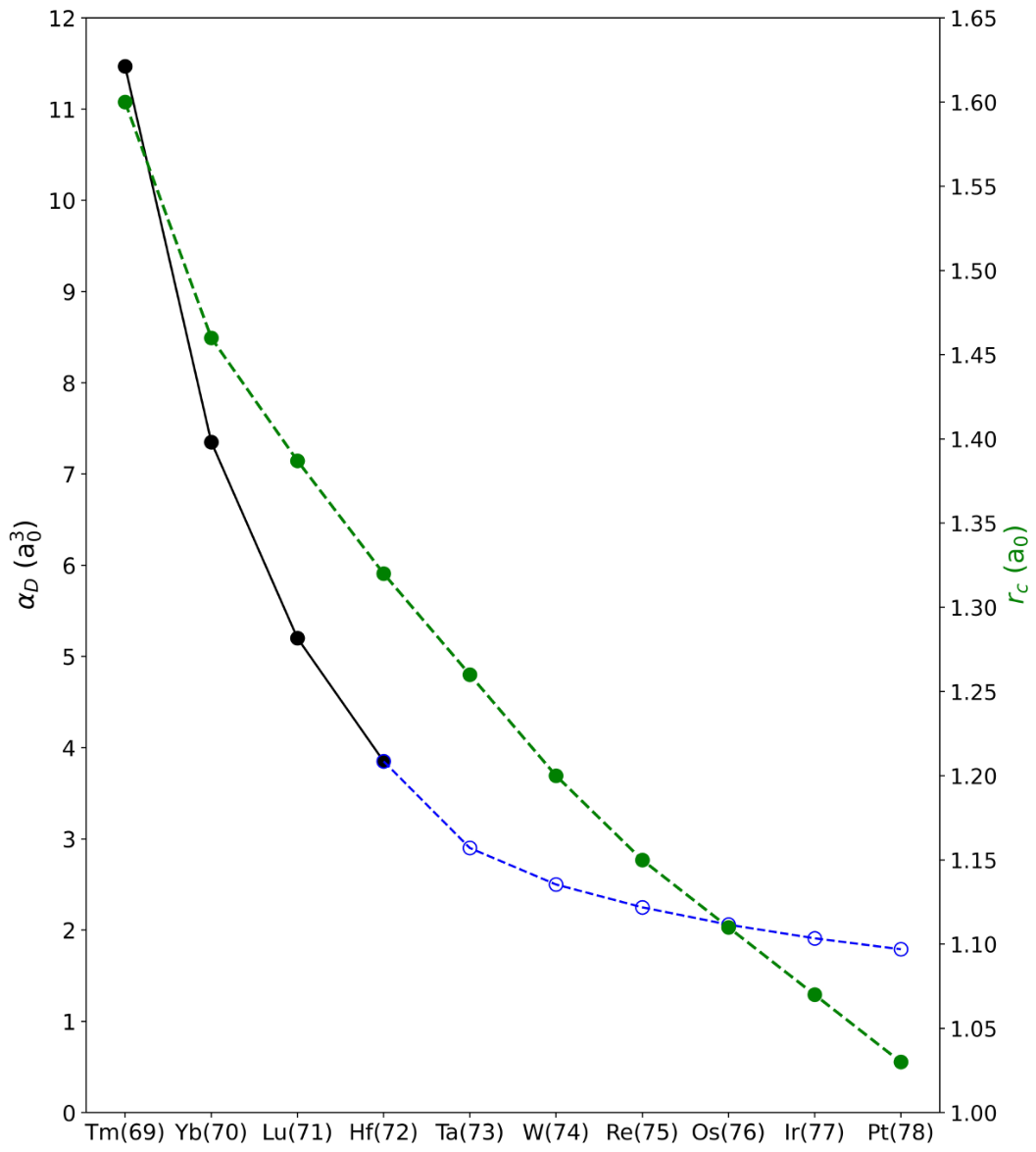
Figure 2.
Evolution of the average energy of the configurations of interest and the core-excited configurations along the Yb isoelectronic sequence.
Figure 2.
Evolution of the average energy of the configurations of interest and the core-excited configurations along the Yb isoelectronic sequence.
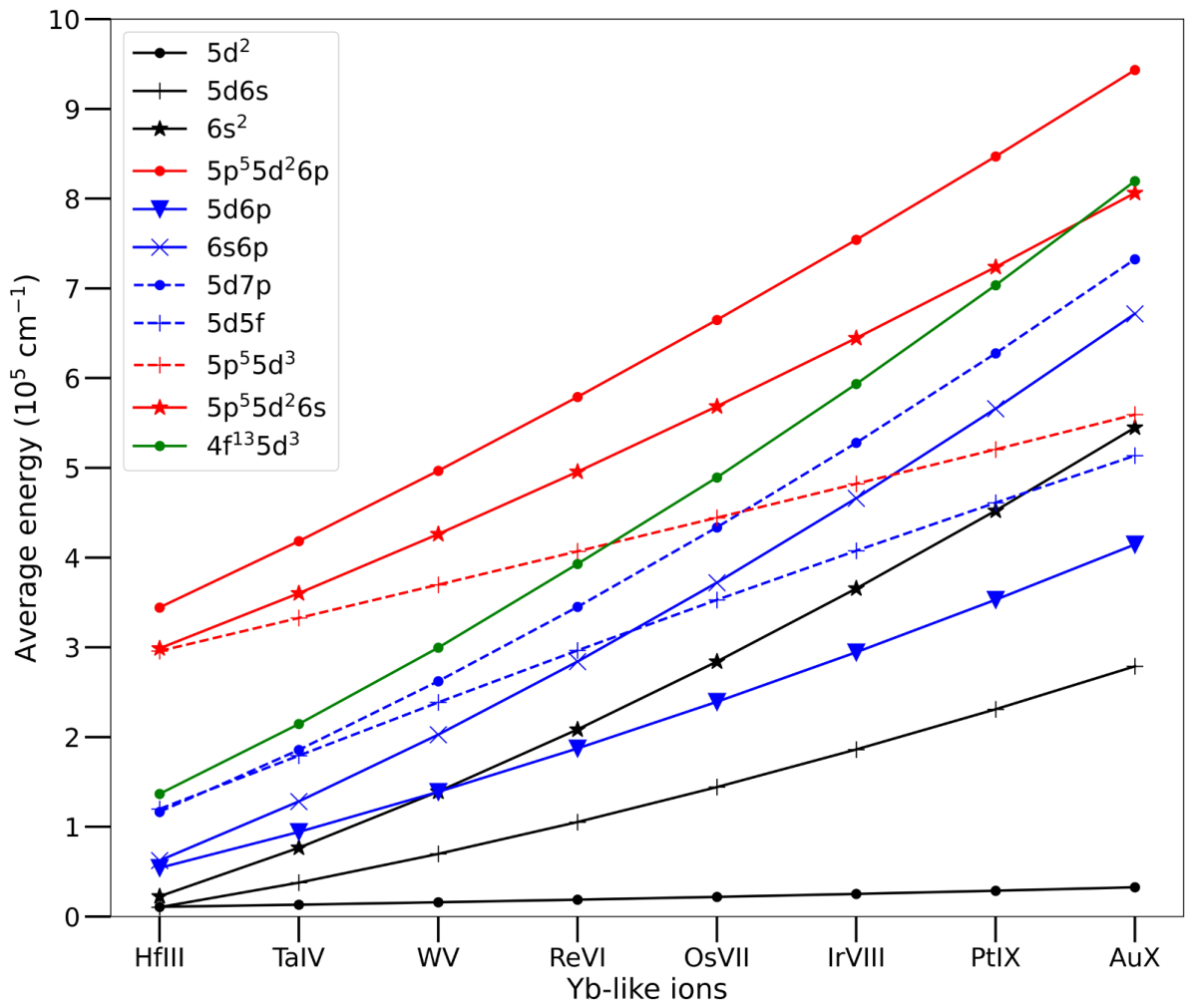
Figure 3.
The energy level distribution of the 5d7p, 5d5f and 4f135d3 odd configurations for Ta IV and W V.
Figure 3.
The energy level distribution of the 5d7p, 5d5f and 4f135d3 odd configurations for Ta IV and W V.
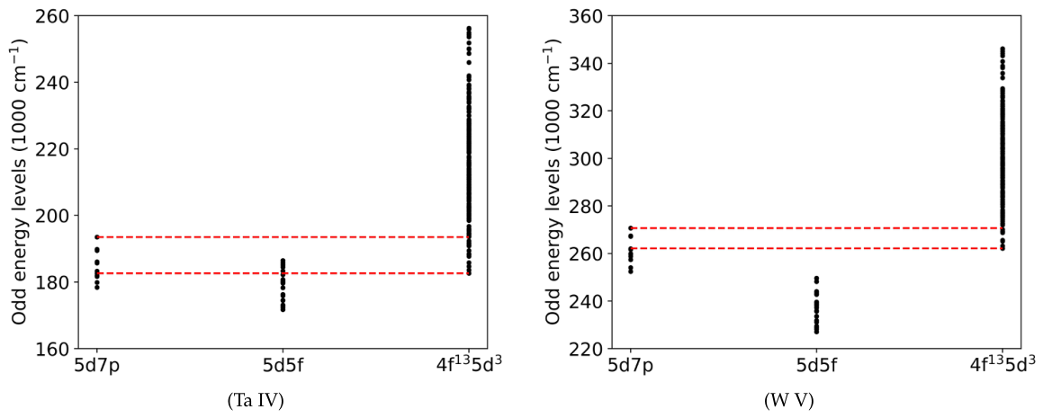
Figure 4.
The core correlation effects on the -values computed with the HFR+CPOL and the HFR(CV) models in Ta IV for the 221 observed lines.
Figure 4.
The core correlation effects on the -values computed with the HFR+CPOL and the HFR(CV) models in Ta IV for the 221 observed lines.
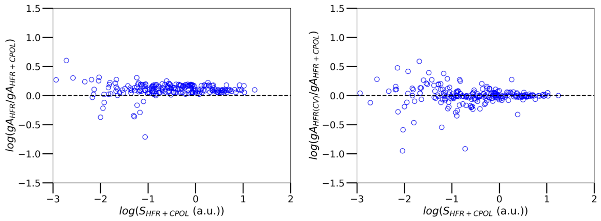
Figure 5.
The core correlation effects on the -values computed with the HFR+CPOL and the HFR(CV) models in W V for all the 193 observed lines.
Figure 5.
The core correlation effects on the -values computed with the HFR+CPOL and the HFR(CV) models in W V for all the 193 observed lines.
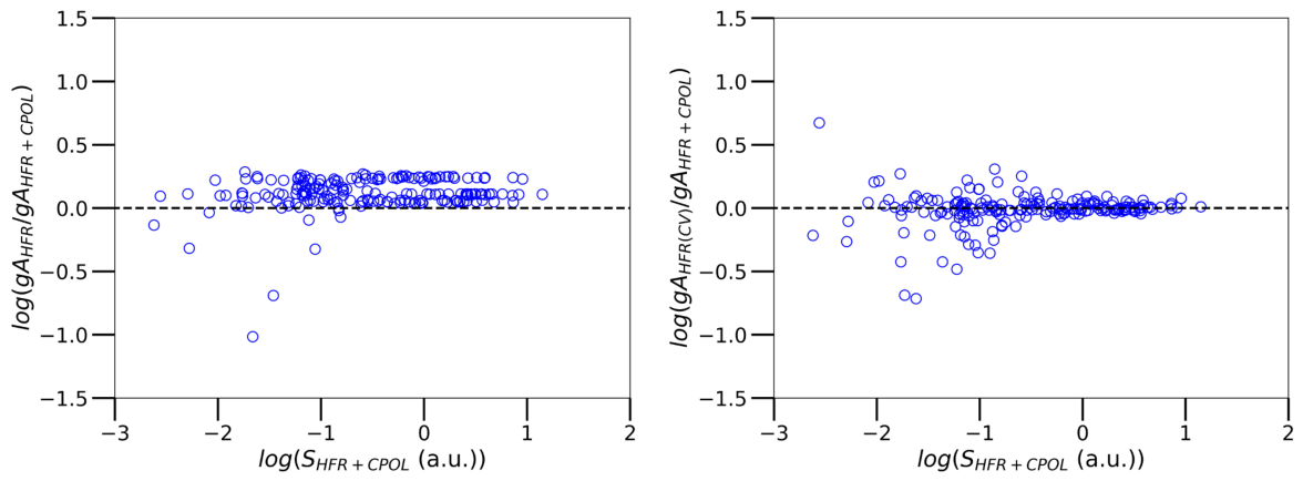
Figure 6.
The core-valence effects on the -values computed with the HFR(CV) model in Re VI, Os VII, Ir VIII and Pt IX for the 112, 147, 129 and 129 lines measured in experiments, respectively.
Figure 6.
The core-valence effects on the -values computed with the HFR(CV) model in Re VI, Os VII, Ir VIII and Pt IX for the 112, 147, 129 and 129 lines measured in experiments, respectively.
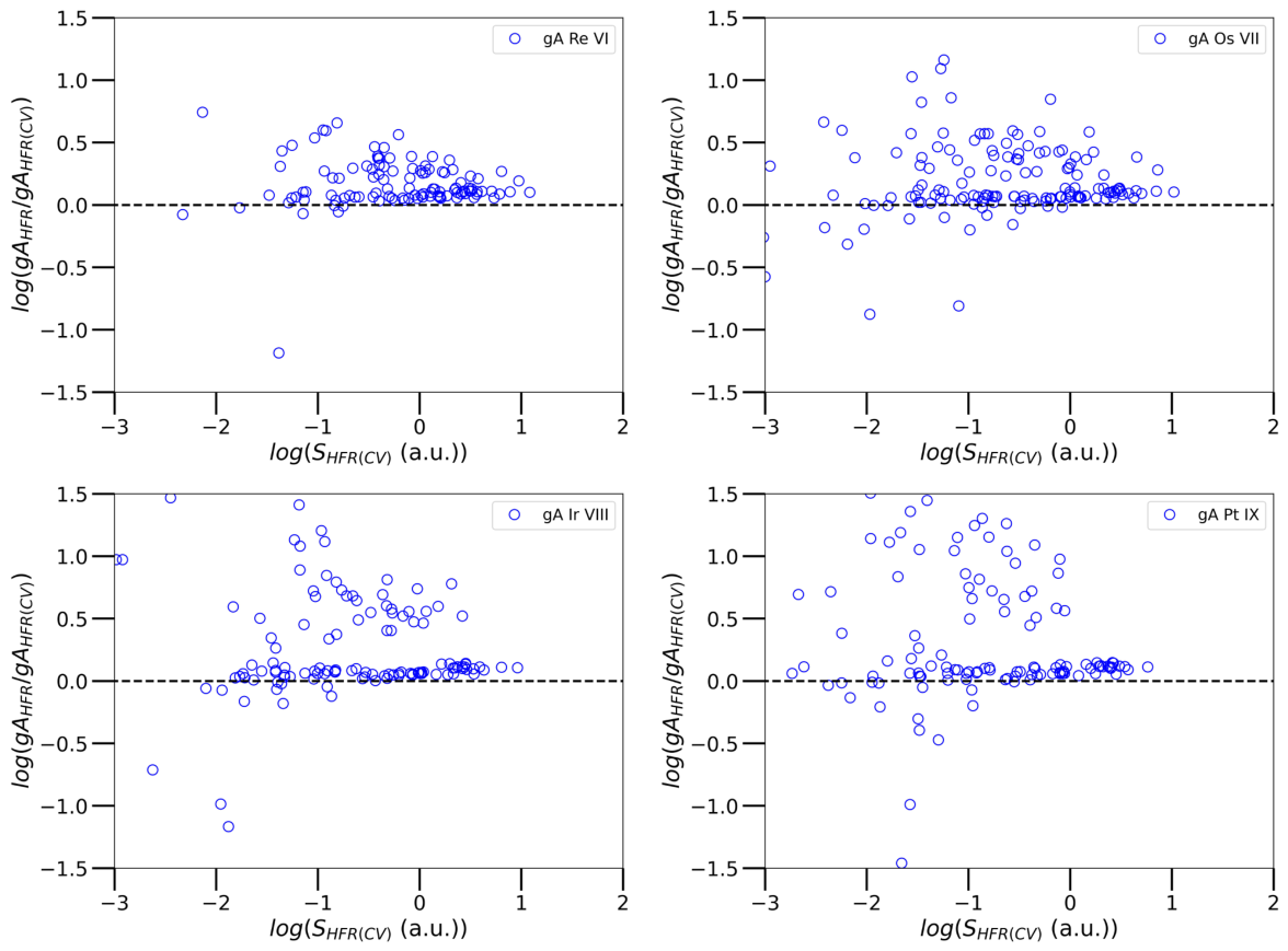
Figure 7.
The large radial part squared of the 4f,5s,5p core orbitals and the 5d,5f,6s,6p,7p valence orbitals that were optimized in the odd parity system with the MCDHF method for Ta IV and Pt IX were plotted as a function of the radius (a0).
Figure 7.
The large radial part squared of the 4f,5s,5p core orbitals and the 5d,5f,6s,6p,7p valence orbitals that were optimized in the odd parity system with the MCDHF method for Ta IV and Pt IX were plotted as a function of the radius (a0).
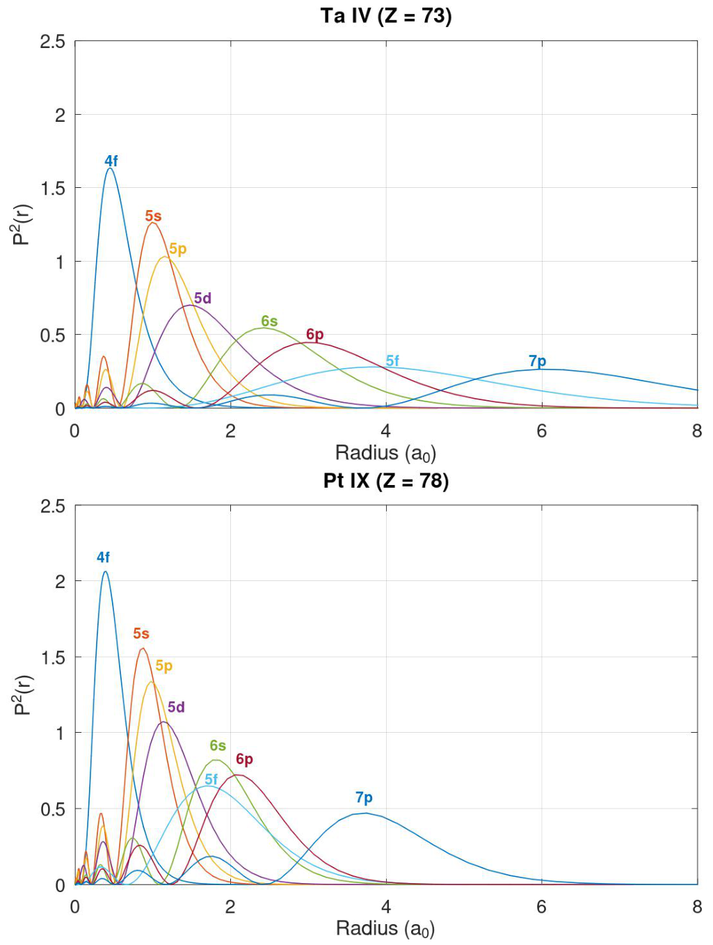
Figure 8.
The radius, (a0), of the 4f,5s,5p core orbitals and the 5d,5f,6s,6p,7p valence orbitals that were obtained in the odd parity system with the MCDHF method for Ta IV up to Pt IX.
Figure 8.
The radius, (a0), of the 4f,5s,5p core orbitals and the 5d,5f,6s,6p,7p valence orbitals that were obtained in the odd parity system with the MCDHF method for Ta IV up to Pt IX.
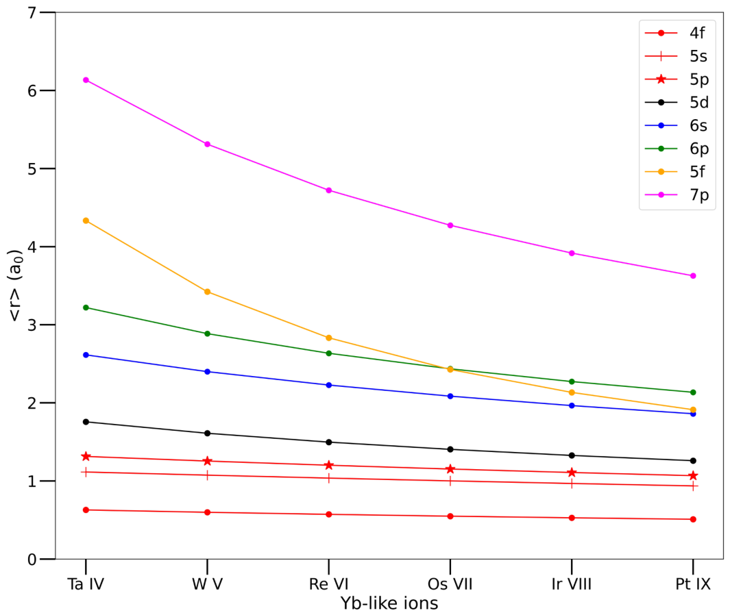
Figure 9.
The cancellation factors as a function of our -values computed with the HFR+CPOL method for the remaining 221 transitions with log() > -4 that are observed in experiments in Ta IV. The dotted line corresponds to = 0.05.
Figure 9.
The cancellation factors as a function of our -values computed with the HFR+CPOL method for the remaining 221 transitions with log() > -4 that are observed in experiments in Ta IV. The dotted line corresponds to = 0.05.
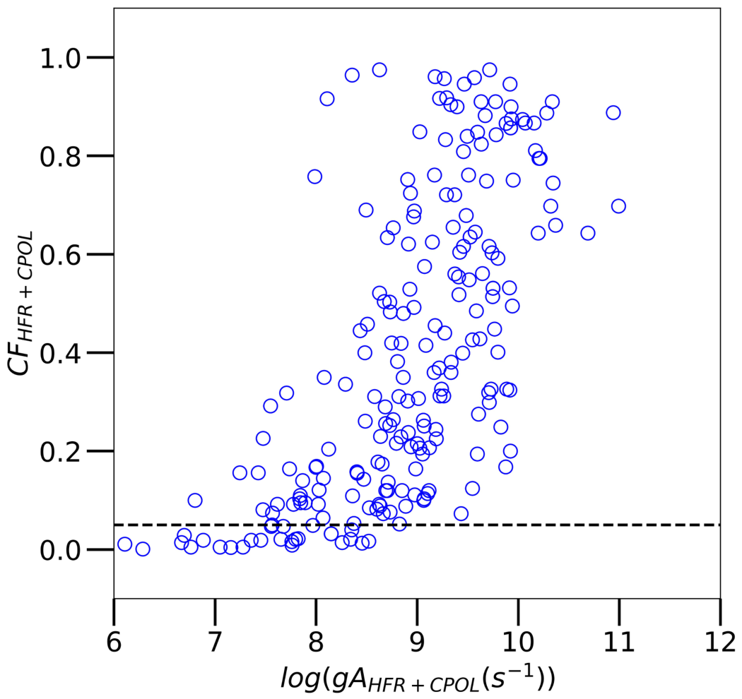
Figure 10.
The uncertainty indicator, dS, as a function of our -values computed with the MCDHF method for all the 355 transitions in Ta IV between the (5d2+5d6s+6s2) even configurations and the (5d6p+6s6p+5d5f+5d7p) odd configurations. The dotted line corresponds to = 0.2.
Figure 10.
The uncertainty indicator, dS, as a function of our -values computed with the MCDHF method for all the 355 transitions in Ta IV between the (5d2+5d6s+6s2) even configurations and the (5d6p+6s6p+5d5f+5d7p) odd configurations. The dotted line corresponds to = 0.2.
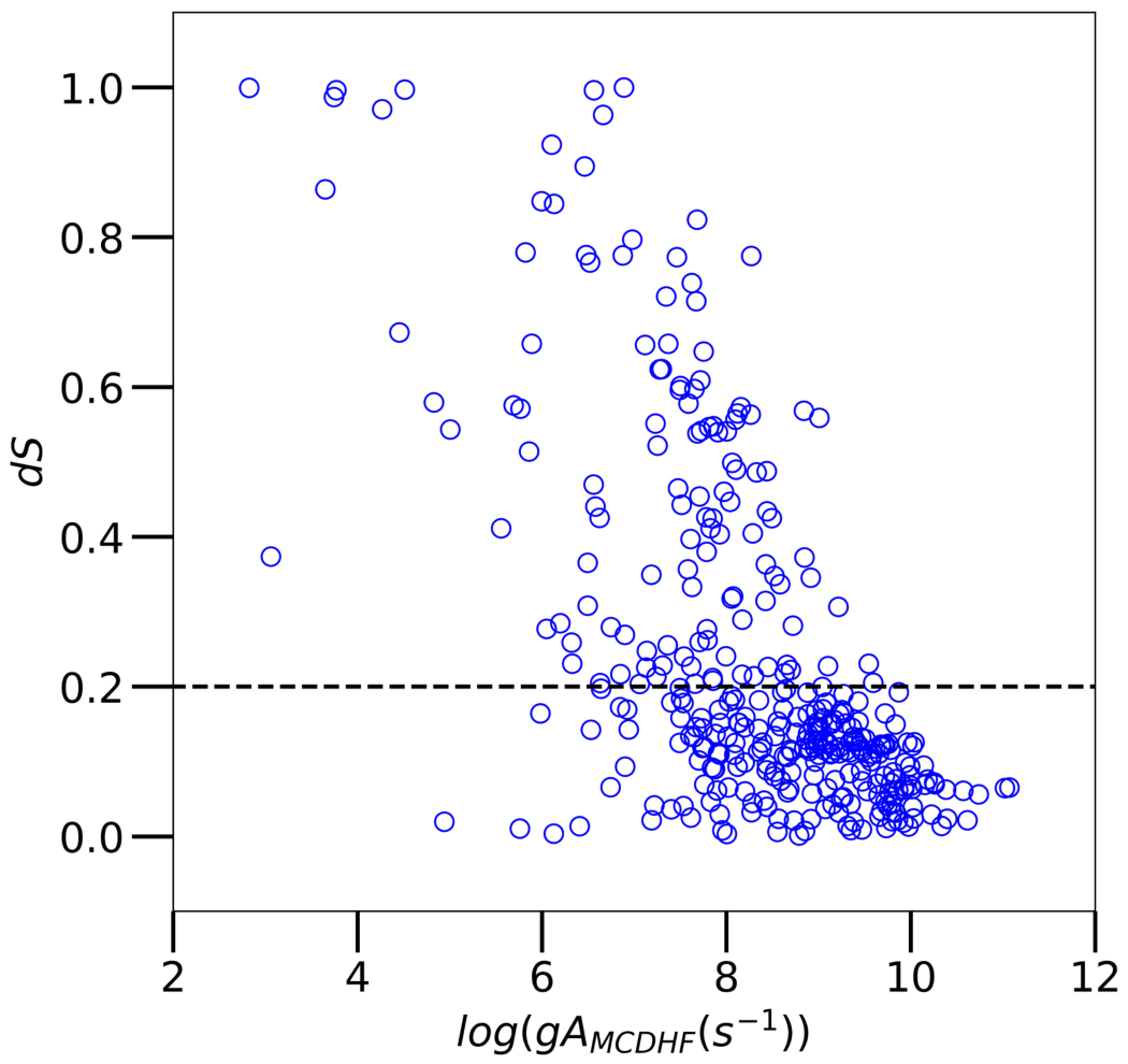
Figure 11.
Comparison between the 354 transition probabilities obtained by the MCDHF-RCI calculations with an interaction DC and DCB Hamiltonian in Ta IV.
Figure 11.
Comparison between the 354 transition probabilities obtained by the MCDHF-RCI calculations with an interaction DC and DCB Hamiltonian in Ta IV.
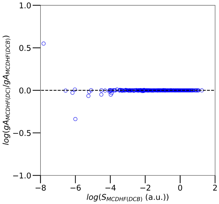
Figure 12.
Comparison between the transition probabilities obtained with the MCDHF-RCI calculations and the HFR+CPOL method for the 221 and 193 transitions observed and selected in Ta IV and W V, respectively. The dotted black line represents the perfect match.
Figure 12.
Comparison between the transition probabilities obtained with the MCDHF-RCI calculations and the HFR+CPOL method for the 221 and 193 transitions observed and selected in Ta IV and W V, respectively. The dotted black line represents the perfect match.
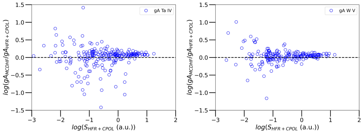
Figure 13.
Comparison between the transition probabilities obtained with the MCDHF-RCI calculations and the HFR(CV) model for all the 112 and 147 transitions observed in Re VI and Os VII, respectively. The solid blue line represents the perfect match.
Figure 13.
Comparison between the transition probabilities obtained with the MCDHF-RCI calculations and the HFR(CV) model for all the 112 and 147 transitions observed in Re VI and Os VII, respectively. The solid blue line represents the perfect match.
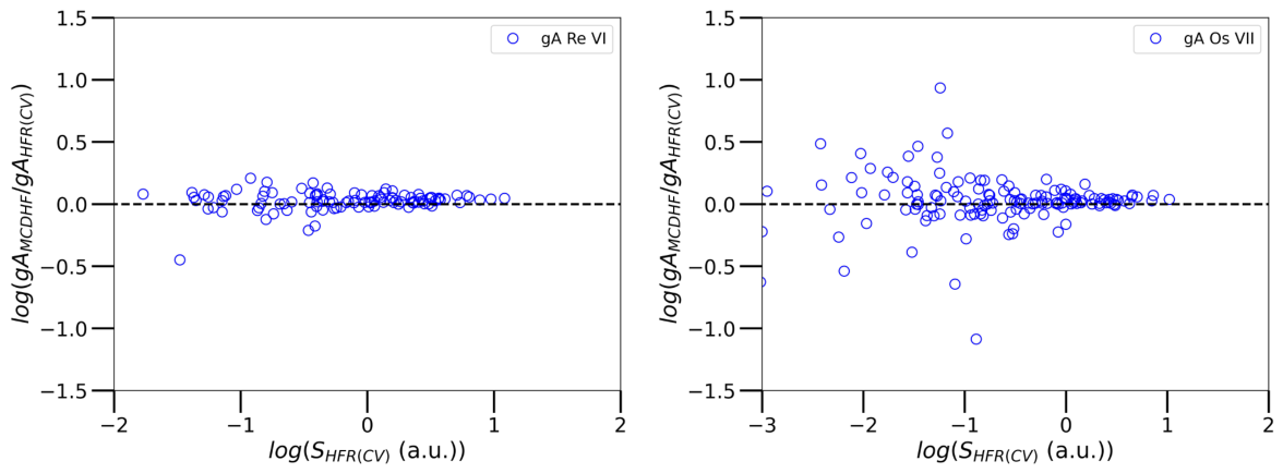
Figure 14.
Comparison between the transition probabilities obtained with the MCDHF-RCI calculations and the HFR(CV) model for all the 125 and 126 transitions observed in Ir VIII and Pt IX, respectively. The solid blue line represents the perfect match.
Figure 14.
Comparison between the transition probabilities obtained with the MCDHF-RCI calculations and the HFR(CV) model for all the 125 and 126 transitions observed in Ir VIII and Pt IX, respectively. The solid blue line represents the perfect match.
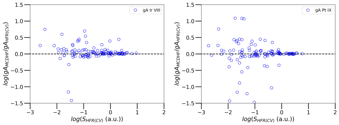
Disclaimer/Publisher’s Note: The statements, opinions and data contained in all publications are solely those of the individual author(s) and contributor(s) and not of MDPI and/or the editor(s). MDPI and/or the editor(s) disclaim responsibility for any injury to people or property resulting from any ideas, methods, instructions or products referred to in the content. |
© 2026 by the authors. Licensee MDPI, Basel, Switzerland. This article is an open access article distributed under the terms and conditions of the Creative Commons Attribution (CC BY) license (http://creativecommons.org/licenses/by/4.0/).
Copyright: This open access article is published under a Creative Commons CC BY 4.0 license, which permit the free download, distribution, and reuse, provided that the author and preprint are cited in any reuse.