

Submitted:
04 August 2026
Posted:
04 August 2026
You are already at the latest version
Abstract
This paper outlines a methodology for using Ultraviolet-Visible (UV-Vis) spectroscopy to measure the concentration of the primary nutrients (N, P, K) and calcium (Ca) for managing hydroponics fertigation solutions and is an extension of previous work presented by the team at GreenSys 2025. This project focuses on supplanting electrical conductivity (EC) as the go-to for inline control of the nutrient mixtures. EC only gives a picture of the total nutrient content of the solution and cannot give insight into the amount of each element present. Others have demonstrated UV-Vis spectroscopy in this measurement role using machine learning for the primary nutrients. The aim here was to improve upon that with a calibration method that is quick, easily reproducible, and usable for an inline controller for near real-time control in hydroponics while also adding support for Ca measurement.
Keywords:
hydroponics
; UV-Vis
; spectroscopy
; fertigation
; NPK
1. Introduction
There is a total of fourteen to eighteen nutrients used in sustaining plants hydroponically; of those, the three primary nutrients focused on in horticulture are nitrogen (N), phosphorous (P), and potassium (K). Calcium (Ca) is also needed in amounts roughly proportional to that of N and K to support plant structures, and for the rest of this paper will also be considered a primary nutrient[1,2,3]. Being able to control each of these directly in near real-time can reduce waste and help improve plant quality and/or yield. Accurate control over individual components of the nutrient solution in real-time has rarely been achieved before; doing so with a single, affordable sensor opens options never seen by growers. This measurement method is the first step on that path.
The goal of this project was to create a calibration and measurement method using a UV-Vis spectrophotometer that can be used for near real-time control of a close loop, recycling hydroponics system. Being able to maintain level of the primary nutrients is critical to maintaining plant health. Currently this role is generally filled using an HPLC offline to allow a person to manually correct for the different rates of nutrient uptake while using EC inline to maintain constant overall dissolved solids, or the systems are drained often enough to not worry about the recycled solution drifting. A UV-Vis spectrophotometer-based solution for controlling the primary nutrients can be in theory placed inline, is non-destructive so there are no consumables, and is easy to operate with minimal training; whereas an HPLC requires a mobile phases solvent which is destructive and uses consumables and typically a skilled operator. While a UV-Vis spectrophotometer has never been demonstrated to also be able to measure the micronutrients, UV-Vis spectroscopy will allow the grower to maintain the growth solution so that HPLC sampling or whole system refreshes can be less frequent. This has been the goal of adapting UV-Vis technology to hydroponics and has been researched in the past, but modern technology has come even further to making this possible[4,5,6]. To that end, this paper focuses on defining a method that is optimized towards this use case. The machine learning method presented by Silva et al. in 2021 showed the ability to quantify N and K concentration, and get qualitative estimates for P [7]. The method presented herein provides a manual process that can be easily implemented by growers without the need for the machine learning aspect, adds support for Ca, and the preliminary data analysis also demonstrates in part why the results they previously achieved were to be expected.
HPLC is commonly used because of its high accuracy and precision relative to other tools that can handle the concentration ranges seen in hydroponics. On its own, a UV-Vis spectrophotometer will likely never be as accurate as the HPLC, but the objective state is instead for the primary nutrients to develop a method that prioritizes the following:
- Detection of a change and the sign on the delta from the target setpoint (i.e. did it increase or decrease);
- An approximation on the magnitude of the change for each element from the setpoint;
- Accuracy in reporting the actual concentrations to an operator is nice to have, but not necessary from a control system implementation standpoint.
2. Materials and Methods
2.1. Fundamentals
Traditionally UV-Vis spectroscopy is based in the Bouguer–Beer–Lambert Law which states the absorption on any single wavelength can be represented as shown in Equation 1 as the absorption (A), times some coefficient (β), times the concentration (x).
A= βx
In a multicomponent mixture this can be further extended as shown in Equation 2, wherein the absorption measured is the summation of all the absorption values for each component of the mixture.
Inherently, this law is not accurate. This proportionality only holds under limited cases. Those limitations are typically met in analytical chemistry by staying at relatively low concentrations, and simple mixtures with very few components. Unfortunately, these constraints are not possible to follow with hydroponics nutrient solutions. It is a complex cocktail of over fourteen different ions and at comparatively high concentrations to those typically measured this way.
The original plan as presented at GreenSys 2025 was to build a model by collecting the absorption spectrum for several common ingredients in hydroponics solution and build a model using that data set. If the Bouguer-Beer-Lambert Law was complete this would have worked, but as is demonstrated in the results section there was too much variability[8,9]. While this theoretical background is the basis of the eventual algorithm presented later, the fact that the hydroponics solution does not meet the limitations for use is why a straightforward implementation of the Bouguer-Beer-Lambert law was ultimately not practical.
2.2. Calibration
Although modeling the hydroponics solution using Equation 2 would have been ideal. The overlaid absorption spectra of the nutrient salts were not directly applicable. The model presented at GreenSys showed general trends that still showed the peaks where they were expected, but the height of the peak in the absorption spectrum did not match the calculated values using the Bouguer-Beer-Labert Law. Fortunately, in a control system the intention would be to keep perturbations small in chemical concentration small so rather than trying to solve for the correct coefficients for each ion of interest to build a model that sums them together, a referential measurement system is employed. An assumption is applied that the primary nutrients are the only parts that will appreciably affect the final absorbance at the selected wavelengths given the proportionally higher concentrations, and that by carefully selecting the wavelengths it is possible to select areas where only two elements dominate at a time. The absorption curves created for each compound informed this wavelength selection, but in practice it would never need to be rerun when calibrating in the future. Using the same wavelengths as were selected later in this process it is possible to calibrate using only calcium nitrate, potassium phosphate, and potassium nitrate. The intent being that these would also be the nutrient salts to be used in a final control system, so they should be readily available. The calibration samples can still be fed to the plants as the test is non-destructive.
2.3. Absorption Spectra of Multiple Solutions
The first step in this process was to get the absorption spectrum for each ion of interest to facilitate wavelength selection and to derive linear models of the three calibration substances. This was done by selecting one element in the substance as primary (i.e. N for any substance containing N), and then creating four solutions that contain roughly 10, 100, 200, and 400 PPM by mass of that element. It should be noted that these will be in ionic forms, so for example N is assumed to be nitrate mostly. These concentrations do not need to be exact since it is assumed the relationship should be linear, but this does cover the full range expected in a typical hydroponics solution to limit the likelihood of having to extrapolate later. Instead, the actual concentration achieved for each was recorded using a mass balance and used to compute the linear fit later for each wavelength measured. Each of these dilutions was placed in a quartz cuvette and then degassed by vibrating in an ultrasonic cleaner to prevent the formation of bubbles during the measurement. It was then placed in the spectrophotometer, and the accompanying software was used to run a wavelength scan from 190-1000 nm. When calibrating in the future a sweep is not required, but it was needed to find the wavelengths of interest. For this experiment a Hogance 30oz Jewelry Cleaner (SJ-H2), a UV-5200PC spectrophotometer and the associated MetaSpec software, a mini-PC running Windows 10, and a Mettler PC 180 (or equivalent) balance scale were used.
The resulting curves across all wavelengths then were smoothed using a wavelet denoising method, specifically the default “wdenoise” in MATLAB R2025b. This smoothing function was only employed to make manual selection of the wavelengths of interest easier when looking at the absorption spectra as a whole. The “noisy” data was still used for the final measurements and calibration. Using wavelet denoising for UV-Vis is not a new concept, and there are debates on which wavelet to use, though trusting the default setting was to focus on optimal smoothing for each sample [10].An overall characteristic curve for each substance was created and plotted against each other to be able to identify the peaks and wavelengths of interest while still being able to gauge the relative heights of each peak. These plots are shown in the “Results” section of this paper.
2.4. Concentration Determination
Four solutions were mixed that approximate Hoagland Solution using a combination of monobasic potassium phosphate, potassium nitrate, calcium nitrate magnesium sulfate, boric acid, manganese sulfate, zinc sulfate, copper sulfate, ammonium molybdate, and chelated iron solutions prepared for the curves mentioned above the final PPM values are shown in Table 1 below. This was then diluted twice, once into a “medium” concentration solution, and once into a low concentration, “dilute” solution, at roughly 30 and 70% dilution respectively. These were again degassed using the ultrasonic cleaner and then run for a scan in the spectrophotometer. The first set, “H1” and its dilutions, were measured at the full range of wavelengths. Once the highest wavelength was selected to be only 210 nm, runs stopped just passed that point to save on time. Concentrations were then calculated using one of the three dilutions of “H1” as a reference and computing the concentration for each of the other solutions from that. Data was also collected for a set of real-world samples from the Controlled Environment Agriculture Center (CEAC) at the University of Arizona.
The final algorithm used the reference sample as a baseline and then scaled its measured values for the primary nutrients off that sample. The ration of the absorption for the sample versus the reference was multiplied by the concentration of the element of interest in the reference. To account for the contribution of N in the sample a weighting function is applied to the absorbance measurement. These weighting functions are shown in Table 2. N and Ca had no weighting applied as the calibration for Ca used calcium nitrate so the weighting function would have double counted the N contribution. The other two used the sum of the expected value from the calibration linear fit based on their initial concentration in the reference sample, plus the expected value from the calibration linear fit for the initial concentration (N0) for the reference sample or the sample concentration (N1) for the sample. The table shows which concentration, and which calibration substance were used when in greater detail.
The function A(X) is defined as the expected absorption for a particular element scaled from the calibration LSRL for a particular substance at a particular wavelength. For example, A([KNO3] @ N1 ) is the expected absorption of the sample concentration (N1) for the LSRL of KNO3. The sample weight for each substance other than N is defined as the sum of the expected absorption of the measured N content (N1) and the expected of absorption of the last known concentration of the item of interest. The reference weight is defined as the sum of the expected absorption of both initial concentrations. In the case of Ca, the height of the N absorption peak at 301nm and at the heigh of the 301nm peak for Ca cannot be separated because the peaks nearly perfectly overlap. As such the sample weight would have been based on the expected absorption of both initial concentrations making the sample and reference weighting equal, so instead no weighting function is applied. Using equation 3 and the associated weighting functions the measured values can be given.
As shown, and based on equation 1, the absorption of the measured sample and the reference are assumed to be proportional. The weighting function is used in place of equation 2 to better approximate the complexity of the hydroponic solution that the traditional Bouguer-Beer-Lambert Law approach would be able to provide.
A1*Ks= A0*Kr
3. Results
3.1. Absorption Spectra of Select Compounds
From the individual substance data collection, the following plots were created. The first, Figure 1, shows an overlay of all of the N containing compounds overlaid on top of each other while showing the wavelengths of interest. From left to right the selected wavelengths are 190.6 nm for finding K, 234.3 nm for N, 235.9 for P, and 301 for Ca. These were created as stated before by measuring all four dilution levels of the compound then applying a least squares regression fit for each wavelength based on the concentration of the element specified in the legend. These were all then plotted using the 100PPM concentration expected value for the associated fit for each wavelength. Ammonium molybdate had a very wide peak that overran everything. This is because the concentrations were so high that the saturation level of the device and the assumptions of the Bouguer-Beer-Lambert law broke down. Fortunately, this is only used as the source for molybdenum so only the smallest trace amount is present in the final solution. The chelation agent in the iron supplement likewise carries N on a very large organic molecule creating a very wide peak, but again it is only present in tiny trace amounts, so it causes minimal impact to the overall absorbance. The UV-5200PC as configured saturates at an absorbance of 3.5. Anything above that is an extrapolation.
The wavelength of 234.4nm was selected for N because the center of the peak at around 210nm is capped by saturating the sensor. Going to where the peak rolled off on the high side eliminated most interfering peaks while avoiding the saturated region. It is however starting to drift into the region that will have an inflated absorbance from the adjacent peak for P, but the nitrate absorbance is expected to be at least an order of magnitude larger and have a higher absorption coefficient, so P will have minimal impact on the estimate. As can be seen more clearly in Figure 2, the nitrate ion also has a clearly defined peak at 300 nm. This peak is tallest for calcium nitrate, indicating that Ca also absorbs over the exact same peak. This is consistent with work with calcium chloride that shows the same peak [11].
Figure 2 shows an overlay of all of the K containing compounds overlaid on top of each other while showing the wavelengths of interest. The only reliable peak is near the very extreme limit of the spectrophotometer. As can be seen with the potassium nitrate curve the nitrate will again dominate. The potassium chloride peak looks more reasonable, but it is unclear whether that peak makes sense. Given the future estimation is referential in nature, scaling off the measured peak at that wavelength for the reference sample, the results for scaling using potassium phosphate and potassium chloride were off by similar amounts of error in the end.
Figure 3 shows an overlay of all of the P containing compounds overlaid on top of each other while showing the wavelengths of interest. There is a clear peak centered at roughly 236 nm. This will be again completely buried under the nitrate peak, but the total absorbance at this wavelength should still increase accordingly. These compounds also indicate that phosphate will absorb at the 190.6 nm being used to find K. The signal for N is again orders of magnitude stronger so, while the results may be refined by accounting for this as a ternary mixture, the estimation method used later is still sufficient for the intended use case in a control system.
Figure 4 shows an overlay of all of the S containing compounds overlaid on top of each other while showing the wavelengths of interest. These are all the remaining solutions that were measured. They are present in fairly small amounts comparatively to K and N so again the absorption at 190.6 nm is ignored. They appear to have a broad peak in the 800 nm range, but it is relatively quiet elsewhere across the spectrum. The selection of 234.4 to find N was selected in part to be past the slight dip in the graph at these lower wavelengths. The method presented in this paper might be able to estimate S as well given the relatively clean peak at the higher wavelengths, but that was outside the scope of this study. The tall Copper peak that aligns with the N peak also would have posed a challenge and was one of the reasons the original modeling method trying to solve for each element directly instead of referentially was unsuccessful. While only a trace amount of copper is present its absorption coefficient is an order of magnitude stronger than P. This meant that being able to detect the trace amount and account for its impact in the estimate was nearly impossible.
3.1. Algorithm and Calibration Method for Implementation
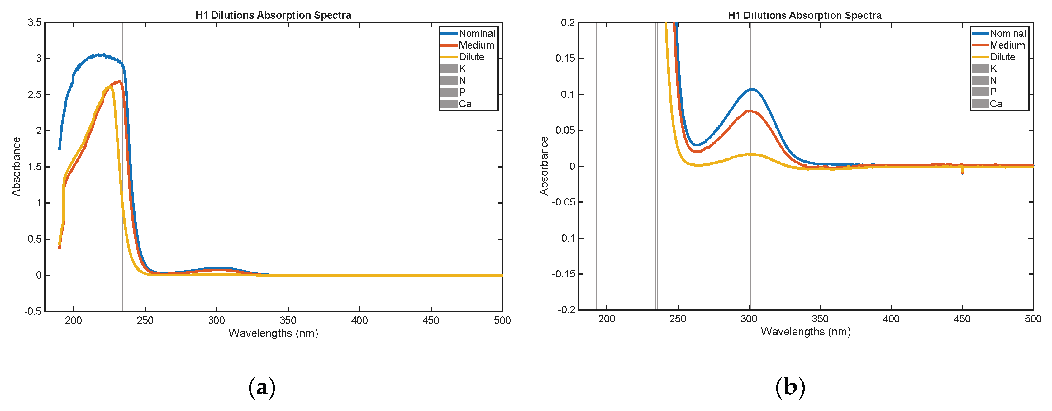
Figure 5 shows the absorption spectra for each dilution of the “H1” sample. The expected peaks are all well-defined, and the selected wavelength for N is visibly in the roll off from the top of the peak in all cases at 234.4 nm. This was selected to avoid the area where the concentrated solution clearly saturated the sensor. The median value of each sample was plotted for each wavelength; this is from three runs wherein each sample in the cuvette was left in the machine and run three times. This served as a sort of voted difference approximation to reduce sampling error. The three lines proved to be nearly identical in all cases up to 900nm. Past that the first run would always return lower after the solution was recently diluted.
As for the other wavelengths, there is a clear peak centered at 301nm where the Ca is being measured. The inflection point just to the right of 190.6 nm is likely from the effect of the K peak. The K ion in theory does not absorb at a wavelength that the selected UV-Vis can measure, but the presence of nitrate and phosphate ions is known to cause a slight red-shift in the peak as is partly observable in Figure 2. Figure 5 does not have any visible artifact for the phosphate peak at 235.9 nm, but given it is such a small absorption value as compared to nitrate peak at the same wavelength, that is to be expected.
Figure 4.
(a) This figure shows the absorption spectrum of a Hoagland-like hydroponics solution, specifically the sample labeled as “H1” throughout this report; (b) this version has been capped at an absorbance of 0.2 to help make artifacts of note in the higher wavelengths more visible.
Figure 4.
(a) This figure shows the absorption spectrum of a Hoagland-like hydroponics solution, specifically the sample labeled as “H1” throughout this report; (b) this version has been capped at an absorbance of 0.2 to help make artifacts of note in the higher wavelengths more visible.
Seeing most of the expected behavior from the individual substance reflected in the overall Hoagland Solution dilutions give confidence that the following procedure is an applicable model for the overall system behavior. This was used to derive the measurements that will follow. Original attempts to use the Bouguer-Beer-Lamber Law directly proved unreliable given that most of the core assumptions were violated. As noted earlier, the final process instead uses weighting functions to estimate the expected impact of a given compound for effecting the change in absorption that is observed. The repeatable portion of the process that would need to be reproduced to make measurements is:
- Prepare pure solutions of potassium nitrate at roughly 10, 100, 200, and 400 PPM N
- Prepare pure solutions of potassium phosphate at roughly 10, 100, 200, and 400 PPM K
- Prepare pure solutions of calcium nitrate at roughly 10, 100, 200, and 400 PPM N
- Create least squares regression line (LSRL) fits for the concentration of K versus absorption in potassium nitrate at 190.6 nm
- Create LSRL for the concentration of N versus absorption in calcium nitrate at 190.6 nm
- Create LSRL for the concentration of P versus absorption in potassium phosphate at 235.9 nm
- Create LSRL for the concentration of N versus absorption in calcium nitrate at 235.9 nm
- Establish a reference baseline by measuring the absorbance of the preferred nutrient solution mix at 190.6, 234.4, 235.9, and 301.0 nm
- Using the LSRL fits from step 4 to compute the weighting values specified in Table 2 and then compute the measured values accordingly
3.2. Performance of Undiluted Concentration Hoagland Solution Reference
The 9-step process described was applied using “H1” as the reference standard. This most closely approximates a scenario where the nutrient solution is fed to the plants, taken up, and then replenished with stock solution matching the original feed. The standard deviations for the primary nutrients as shown in Table 3 for N, P, K are 23, 18, and 26 PPM respectively, with Ca coming in at 11 PPM. The magnitude of the error gets consistently worse as the measured sample gets more diluted with the most dilute, those samples ending in “D” being noticeably further off.
3.3. Performance of Moderate Concentration Hoagland Solution Reference
The 6-step process described was applied using “H1M” as the reference standard. This most closely approximates a scenario where the nutrient solution is fed to the plants, slightly more water than nutrient is taken up, and then replenished with stock solution matching the original feed. The standard deviations for the primary nutrients as shown in Table 4 for N, P, K are 21, 18, and 24 PPM respectively, with Ca coming in at 9.7 PPM. Again, the magnitude of the error gets consistently worse as the measured sample gets further from the reference.
3.4. Performance of Diltue Concentration Hoagland Solution Reference
The 6-step process described was applied using “H1D” as the reference standard. This most closely approximates a scenario where the nutrient solution is fed to the plants, and significantly more water than nutrient is taken up, and then replenished with stock solution matching the original feed. The standard deviations for the primary nutrients as shown in Table 5 for N, P, K are 39, 16, and 30 PPM respectively, with Ca coming in at 29 PPM. Again, the magnitude of the error gets consistently worse as the measured sample gets further from the reference. This is by far the worst performance of options for which reference to pick. This is likely because in the heavily diluted case the signal to noise ratio of the UV-Vis measurements for the reference is also the worst. The phosphate peak would be nearly nonexistent, and the peaks for Ca and K would be much smaller than those from the concentrated sample. This turns the entire problem into one of extrapolation, which is known to be inaccurate.
3.5. Performance of Using Greenhouse Initial Solution as a Reference
This section presents the measurements from real-world samples from University of Arizona greenhouses. Those in Table 6 that start with “TG” were taken from the CEAC teaching greenhouse. “TG0” is taken directly from the solution being fed to the plants and the rest are taken at the end of the row matching the number. “RT1” was taken from the rooftop greenhouse after it had been running for about 3 months in a closed loop.
4. Discussion
In the ideal case, where the measurements were performed using reagent grade nutrient salts and deionized water the 6-step method proposed was able to deliver results similar to those expected after looking at the success of the machine learning algorithm presented by Silva et al. Their results were within 6.7% and 3.8% for N and K respectively while also getting qualitative values for P [7]. At roughly 25/150 PPM, the standard deviation in the results for the concentrated and moderate reference were able to get within roughly 17% using the simplified approach described in this paper. This method also showed promising results under these controlled conditions for P and Ca, adding further functional improvements to the analysis. Machine learning is still expected to be more precise as there is a lot more data being analyzed at once.
The 6-step method in this paper benefits from working with significantly less data than an algorithm that relies on sweeping a multitude of wavelengths (as is done in the machine learning based approaches). Requiring only four wavelengths and three calibration substances, plus a reference solution, this method requires very little time to set up as well. Assuming concentrated stock solutions of these three are readily available, which is to be expected as they can be used directly to mix Hoagland Solution, it is simply a matter of diluting the sample to get the calibration curve. Using only four wavelengths, this is also not computationally or memory intensive. For long term data storage only twelve floating point numbers are required from the calibration data for the algorithm, with a similarly small number of summation and multiplication operations required during operation. This means adjustments to the nutrient solution can easily be made on the timescale of multiple times every hour. It is still recommended that a blank of deionized water be used to recalibrate the UV-Vis regularly, and that if the device selected has a recalibration procedure for the wavelength selection it should be run regularly as well. For the purposes of these experiments, the UV-Vis itself was recalibrated daily, taking roughly 30 minutes of down time.
The real-world results were less encouraging, and further study is likely required. The three most egregious misses were “TG3”, “TG5”, and “RT1”. For “RT1” the most likely culprit is the severe depletion of the primary nutrients and the very high sulfate concentration. At higher concentrations the sulfate has been demonstrated to absorb at wavelengths more similar to the other primary nutrients [12]. For “TG3” the much higher concentration of K is also likely a contributing factor. This is much higher than the reference value and calibration data set were designed to work with without significant extrapolation. In the case of “TG5” there is no obvious culprit to explain why it was comparatively so far off from the performance in the idealized case. The other contributing factor that would also need further examination is the plant exudates. One of the other big differences from the idealized case was the use of tap water for the nutrient solution, and the use of a different chelate for the iron supplement. The iron supplement was also present in much higher concentrations in the real-world samples than in the idealized laboratory case. The chelate was also seen to degrade in UV light as expected, so multiple runs were needed, instead of just the first three measurements, to get the measurements to stabilize instead of being lower with successive passes.
All of these considerations can mostly be handled by careful implementation of what modified Hoaglan Solution to use, and careful control system design. As for the top objectives of this method, the idealized cases demonstrated most of the desired behavior and would allow the control system to make corrections accurately, but only giving minimal precision as to what the true measured value is for reporting to the operator. The real-world samples were less promising as they often did not show decreases in N content when they should have. Given the weighting functions, this may also have further contributed to the inaccuracy of those measurements. Further study into accounting for S, plant exudates, improvements on the weighting functions (possibly including dynamically adjusting the weighting function based on HPLC measurements), and the implementation of better machine learning algorithms instead of this simplified method would all be good avenues of research to pursue next.
Supplementary Materials
The following supporting information can be downloaded at: https://github.com/mikezankel/UV_Vis_PrimaryNutrient, for source code, data, and all provided figures and tables.
Author Contributions
Conceptualization, Michael Zankel; methodology, Michael Zankel; software, Michael Zankel; validation, Michael Zankel, Dr. Joel Cuello, Dr. Triston Hooks, Dr. Murat Kacira, and Dr. M. Leandro Heien; formal analysis, Michael Zankel; investigation, Michael Zankel; resources, Dr. M. Leandro Heien; data curation, Michael Zankel; writing—original draft preparation, Michael Zankel; writing—review and editing, Michael Zankel; visualization, Michael Zankel; supervision, Dr. Joel Cuello, Dr. Triston Hooks, Dr. Murat Kacira, and Dr. M. Leandro Heien.; project administration, Michael Zankel. All authors have read and agreed to the published version of the manuscript.
Funding
This research received no external funding.
Data Availability Statement
All collected data is available at https://github.com/mikezankel/UV_Vis_PrimaryNutrient/raw_data
Conflicts of Interest
The authors declare no conflicts of interest.
Abbreviations
The following abbreviations are used in this manuscript:
| HPLC | High-pressure Liquid Chromatograph |
| LSRL | Least-squares Rgression Line |
| UV | Ultra-Violet |
References
- White, P.J.; Brown, P.H. Plant Nutrition for Sustainable Development and Global Health. Ann. Bot. 2010, 105, 1073–1080. [CrossRef]
- Hoagland, D.R. The Water-Culture Method for Growing Plants without Soil.
- Hydroponics - A Standard Methodology for Plant Biological Researches; Asao, T., Ed.; InTech, 2012; ISBN 978-953-51-0386-8.
- On-Line Monitoring of Water Quality and Plant Nutrients in Space Applications Based on Photodiode Array Spectrometry Available online: https://www.sae.org/publications/technical-papers/content/911361/ (accessed on 13 March 2024).
- Spectroscopic Techniques Developed for NASA Used for Commercial Water Treatment Processes Available online: https://www.spectroscopyonline.com/view/spectroscopic-techniques-developed-nasa-used-commercial-water-treatment-processes (accessed on 13 March 2024).
- Silva, F.M.; Queirós, C.; Pinho, T.; Boaventura, J.; Santos, F.; Barroso, T.G.; Pereira, M.R.; Cunha, M.; Martins, R.C. Reagent-Less Spectroscopy towards NPK Sensing for Hydroponics Nutrient Solutions. Sens. Actuators B Chem. 2023, 395, 134442. [CrossRef]
- Silva, A.F.; Löfkvist, K.; Gilbertsson, M.; Os, E.V.; Franken, G.; Balendonck, J.; Pinho, T.M.; Boaventura-Cunha, J.; Coelho, L.; Jorge, P.; et al. Hydroponics Monitoring through UV-Vis Spectroscopy and Artificial Intelligence: Quantification of Nitrogen, Phosphorous and Potassium. In Proceedings of the The 1st International Electronic Conference on Chemical Sensors and Analytical Chemistry; MDPI, June 30 2021; p. 88.
- Mayerhöfer, T.G.; Pahlow, S.; Popp, J. The Bouguer-Beer-Lambert Law: Shining Light on the Obscure. ChemPhysChem 2020, 21, 2029–2046. [CrossRef]
- Beer’s Law – Why Absorbance Depends (Almost) Linearly on Concentration Available online: https://chemistry-europe.onlinelibrary.wiley.com/doi/epdf/10.1002/cphc.201801073?saml_referrer (accessed on 15 August 2025).
- Sohrabi, M.R.; Mirzabeygi, V.; Davallo, M. Use of Continuous Wavelet Transform Approach for Simultaneous Quantitative Determination of Multicomponent Mixture by UV–Vis Spectrophotometry. Spectrochim. Acta. A. Mol. Biomol. Spectrosc. 2018, 201, 306–314. [CrossRef]
- Yousef, N.; Mawad, A.; Abeed, A. Enhancement the Cellulase Activity Induced by Endophytic Bacteria Using Calcium Nanoparticles. Curr. Microbiol. 2019, 76, 346–354. [CrossRef]
- Nagabhushana, H.; Nagaraju, G.; Nagabhushana, B.M.; Shivakumara, C.; Chakradhar, R.P.S. Hydrothermal Synthesis and Characterization of CaSO4 Pseudomicrorods. Philos. Mag. Lett. 2010, 90, 289–298. [CrossRef]
Figure 1.
(a) This figure shows the set of nitrogen containing compounds measured overlaid with the wavelengths of interest; (b) this version has been capped at an absorbance of 0.2 to help make artifacts of note in the higher wavelengths more visible.
Figure 1.
(a) This figure shows the set of nitrogen containing compounds measured overlaid with the wavelengths of interest; (b) this version has been capped at an absorbance of 0.2 to help make artifacts of note in the higher wavelengths more visible.
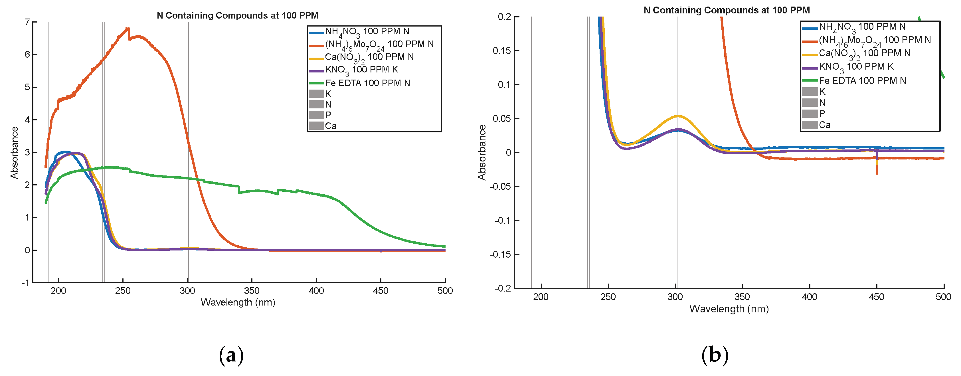
Figure 2.
(a) This figure shows the potassium containing compounds measured overlaid with the wavelengths of interest; (b) this version has been capped at an absorbance of 0.2 to help make artifacts of note in the higher wavelengths more visible.
Figure 2.
(a) This figure shows the potassium containing compounds measured overlaid with the wavelengths of interest; (b) this version has been capped at an absorbance of 0.2 to help make artifacts of note in the higher wavelengths more visible.
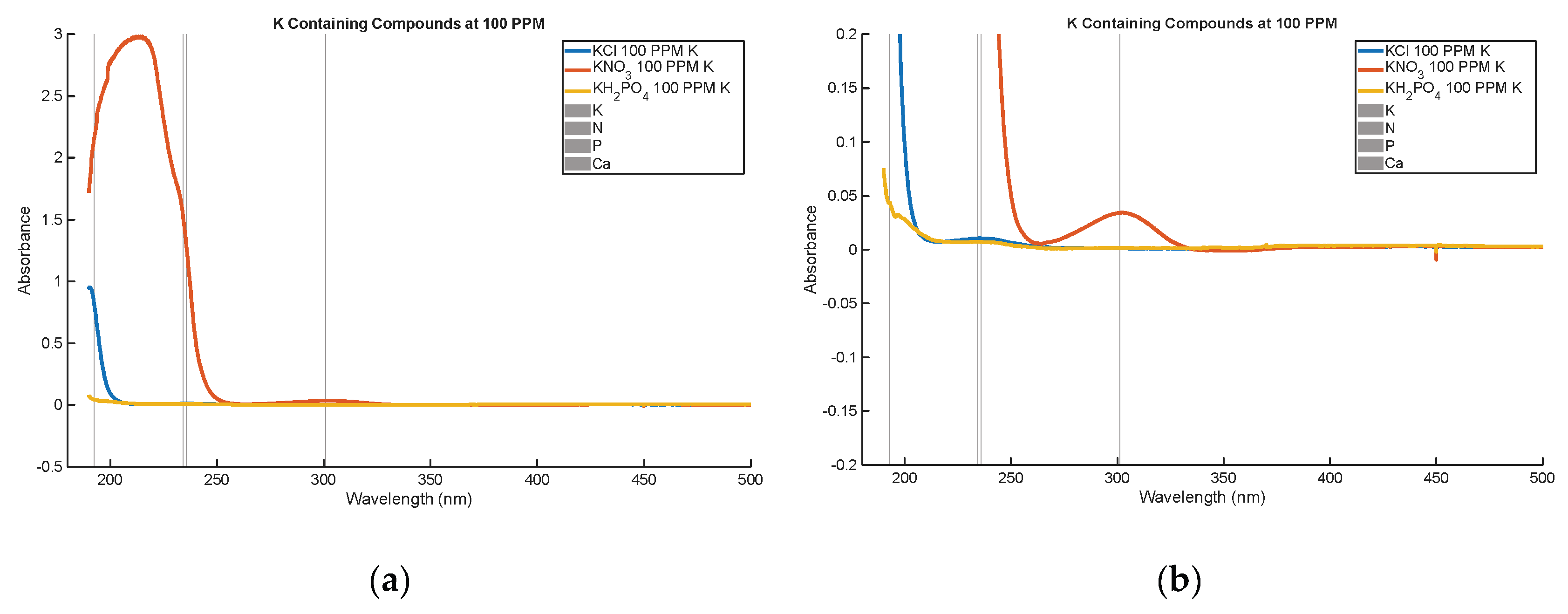
Figure 3.
This figure shows the phosphate containing compounds measured overlaid with the wavelengths of interest.
Figure 3.
This figure shows the phosphate containing compounds measured overlaid with the wavelengths of interest.
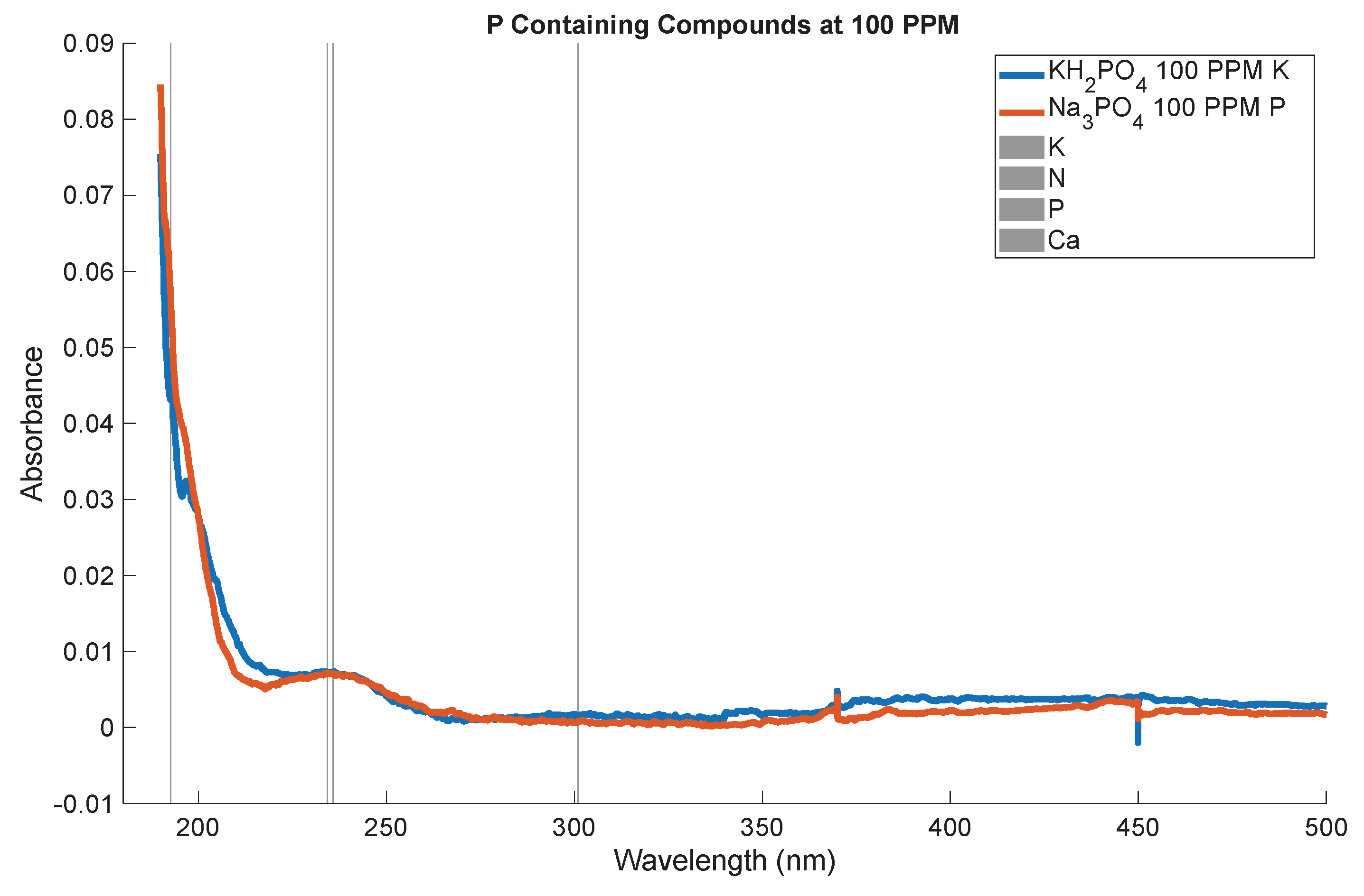
Figure 4.
(a) This figure shows the sulfate containing compounds measured overlaid with the wavelengths of interest; (b) this version has been capped at an absorbance of 0.2 to help make artifacts of note in the higher wavelengths more visible.
Figure 4.
(a) This figure shows the sulfate containing compounds measured overlaid with the wavelengths of interest; (b) this version has been capped at an absorbance of 0.2 to help make artifacts of note in the higher wavelengths more visible.
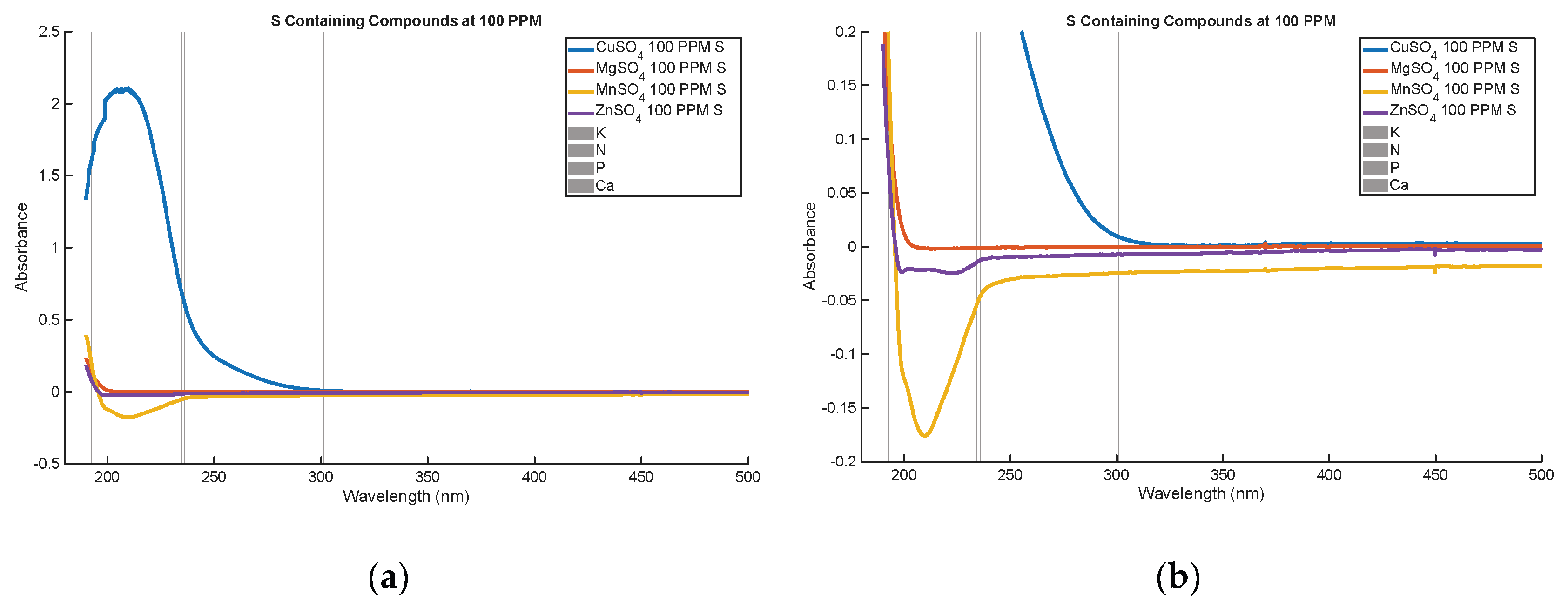

Table 1.
This table shows the concentrations of the element of interest in PPM. Ions listed are the dominant ion in the solution, although ammonium ions are mentioned, it is only a trace amount from the ammonium molybdate. The concentrations given are however for the element, not the ion. The first 4 are the concentrated Hoaglan-like samples that were created, the ones ending in “M” were diluted by roughly 30 percent, and the ones ending in “D” were diluted by roughly 70 percent. The sample CE0 was a sample of regular tap water taken from the University of Arizona Controlled Environment Agriculture Center (CEAC), the sample RT1 was taken from the University of Arizona’s Rooftop Greenhouse after it had been left running closed-loop for a few months. The samples TG1-7 were taken from the CEAC teaching greenhouse after a stock solution of TG0 was fed to the crops in single pass.
Table 1.
This table shows the concentrations of the element of interest in PPM. Ions listed are the dominant ion in the solution, although ammonium ions are mentioned, it is only a trace amount from the ammonium molybdate. The concentrations given are however for the element, not the ion. The first 4 are the concentrated Hoaglan-like samples that were created, the ones ending in “M” were diluted by roughly 30 percent, and the ones ending in “D” were diluted by roughly 70 percent. The sample CE0 was a sample of regular tap water taken from the University of Arizona Controlled Environment Agriculture Center (CEAC), the sample RT1 was taken from the University of Arizona’s Rooftop Greenhouse after it had been left running closed-loop for a few months. The samples TG1-7 were taken from the CEAC teaching greenhouse after a stock solution of TG0 was fed to the crops in single pass.
| Nutrients | ||||||||||||
|---|---|---|---|---|---|---|---|---|---|---|---|---|
| Element | B | Ca | Cu | Fe | K | Mg | Mn | Mo | N | P | S | Zn |
| Primary Ion | H2BO3- | Ca2+ | Cu2+ | Fe2+ | K+ | Mg2+ | Mn2+ | MoO42- | NH3+, NO3- | PO43- | SO42- | Zn2+ |
| H1 | 0.48 | 170 | 0.069 | 0.29 | 140 | 33 | 1.1 | 0.1 | 160 | 28 | 44 | 0.19 |
| H1A | 0.41 | 200 | 0.06 | 0.25 | 130 | 28 | 0.92 | 0.09 | 180 | 24 | 38 | 0.16 |
| H2 | 0.63 | 170 | 0.051 | 1 | 160 | 39 | 1.5 | 0.022 | 160 | 41 | 53 | 0.39 |
| H2A | 0.57 | 150 | 0.047 | 0.93 | 200 | 36 | 1.3 | 0.02 | 140 | 78 | 48 | 0.36 |
| H1M | 0.36 | 120 | 0.052 | 0.22 | 110 | 24 | 0.79 | 0.078 | 120 | 21 | 33 | 0.14 |
| H1AM | 0.31 | 150 | 0.045 | 0.19 | 94 | 21 | 0.69 | 0.068 | 130 | 18 | 29 | 0.12 |
| H2M | 0.43 | 110 | 0.035 | 0.7 | 110 | 27 | 1 | 0.015 | 110 | 28 | 36 | 0.27 |
| H2AM | 0.31 | 82 | 0.026 | 0.51 | 110 | 19 | 0.72 | 0.011 | 78 | 43 | 26 | 0.19 |
| H1D | 0.096 | 34 | 0.014 | 0.059 | 29 | 6.6 | 0.21 | 0.021 | 32 | 5.6 | 8.9 | 0.038 |
| H1AD | 0.11 | 56 | 0.017 | 0.07 | 35 | 7.9 | 0.25 | 0.025 | 49 | 6.6 | 11 | 0.046 |
| H2D | 0.15 | 40 | 0.013 | 0.25 | 40 | 9.5 | 0.36 | 0.0054 | 38 | 10 | 13 | 0.095 |
| H2AD | 0.15 | 40 | 0.012 | 0.25 | 53 | 9.4 | 0.35 | 0.0053 | 38 | 21 | 13 | 0.094 |
| CE0 | 0.07 | 60 | 0 | 0 | 1.9 | 4.1 | 0 | 0.01 | 8.7 | 0.04 | 8 | 0.03 |
| RT1 | 0.85 | 180 | 0.48 | 4.2 | 0.99 | 88 | 0.3 | 0.01 | 8.6 | 2.9 | 520 | 5.7 |
| TG0 | 0.46 | 150 | 0.09 | 1.5 | 200 | 57 | 0.65 | 0.06 | 120 | 39 | 99 | 0.25 |
| TG1 | 0.54 | 170 | 0.11 | 1.8 | 230 | 65 | 0.73 | 0.06 | 150 | 45 | 110 | 0.34 |
| TG3 | 1.3 | 270 | 0.22 | 7.3 | 650 | 170 | 0.28 | 0.29 | 70 | 49 | 260 | 0.36 |
| TG5 | 0.4 | 130 | 0.09 | 1.3 | 170 | 47 | 0.51 | 0.05 | 98 | 31 | 80 | 0.28 |
| TG7 | 0.89 | 240 | 0.15 | 4 | 280 | 120 | 0.17 | 0.09 | 170 | 36 | 220 | 0.14 |
Table 2.
This table shows the wavelength of interest and the weighting function applied to the measured absorption to estimate the impact of each compound at that wavelength. The function A(X) is defined as the expected absorption for a particular element scaled from the calibration LSRL for a particular substance at a particular wavelength. For example, A([KNO3] @ N1 ) is the expected absorption of the sample concentration (N1) for the LSRL of KNO3.
Table 2.
This table shows the wavelength of interest and the weighting function applied to the measured absorption to estimate the impact of each compound at that wavelength. The function A(X) is defined as the expected absorption for a particular element scaled from the calibration LSRL for a particular substance at a particular wavelength. For example, A([KNO3] @ N1 ) is the expected absorption of the sample concentration (N1) for the LSRL of KNO3.
| Element | Wavelength (nm) | Sample Weight (Ks) | Reference Weight (Kr) |
|---|---|---|---|
| N | 234.4 | 1 | 1 |
| P | 235.9 | A([KNO3] @ N1 )+ A([KH2PO4] @ P0) | A([KNO3] @ N0) + A([KH2PO4] @ P0) |
| K | 190.6 | A([Ca(NO3)2] @ N1) +A([KH2PO4] @ K0) | A([Ca(NO3)2] @ N0) + A([KH2PO4] @ K0) |
| Ca | 301.0 | 1 | 1 |
Table 3.
This tables shows all the results when using the sample “H1”, which was undiluted Hoagland Solution, as a reference. The columns ending in the “0” subscript are the initial concentration. The columns ending in “T” are the expected value from when the solution was mixed and measured using a mass balance. The values ending in “1” are the measurement derived from the algorithm that uses the absorptions. These values are all in PPM. The last row as “StdDev” is the standard deviation in the measurement, whereas all other values in the “Sample” column are the sample identifiers referenced elsewhere in this document. The columns ending in “P” are the percentage error; although these percentages are usually given unsigned, negative values are under the target value, whereas positive values are overestimates.
Table 3.
This tables shows all the results when using the sample “H1”, which was undiluted Hoagland Solution, as a reference. The columns ending in the “0” subscript are the initial concentration. The columns ending in “T” are the expected value from when the solution was mixed and measured using a mass balance. The values ending in “1” are the measurement derived from the algorithm that uses the absorptions. These values are all in PPM. The last row as “StdDev” is the standard deviation in the measurement, whereas all other values in the “Sample” column are the sample identifiers referenced elsewhere in this document. The columns ending in “P” are the percentage error; although these percentages are usually given unsigned, negative values are under the target value, whereas positive values are overestimates.
| Sample | NT | KT | PT | CaT | ST | N1 | K1 | P1 | Ca1 | Np | Kp | Pp | Cap |
|---|---|---|---|---|---|---|---|---|---|---|---|---|---|
| H1* | 160 | 140 | 28 | 170 | 44 | 160 | 140 | 28 | 170 | 0 | 0 | 0 | 0 |
| H2 | 160 | 160 | 41 | 170 | 53 | 160 | 140 | 28 | 160 | 0 | -13 | -32 | -6 |
| H1A | 180 | 130 | 24 | 200 | 38 | 160 | 150 | 28 | 170 | -11 | 15 | 17 | -15 |
| H2A | 140 | 200 | 78 | 150 | 48 | 160 | 130 | 27 | 150 | 14 | -35 | -65 | 0 |
| H1M | 120 | 110 | 21 | 120 | 33 | 140 | 100 | 21 | 120 | 17 | -9 | 0 | 0 |
| H2M | 110 | 110 | 28 | 110 | 36 | 140 | 97 | 21 | 110 | 27 | -12 | -25 | 0 |
| H1AM | 130 | 94 | 18 | 150 | 29 | 150 | 110 | 24 | 130 | 15 | 17 | 33 | -13 |
| H2AM | 78 | 110 | 43 | 82 | 26 | 120 | 73 | 14 | 83 | 54 | -34 | -67 | 1.2 |
| H1D | 32 | 29 | 6 | 34 | 9 | 50 | 23 | 4 | 26 | 56 | -21 | -34 | -24 |
| H2D | 38 | 40 | 10 | 40 | 13 | 63 | 35 | 5 | 39 | 66 | -13 | -49 | -3 |
| H1AD | 49 | 35 | 7 | 56 | 11 | 73 | 40 | 6 | 46 | 49 | 14 | -5 | -18 |
| H2AD | 38 | 53 | 21 | 40 | 13 | 60 | 34 | 5 | 39 | 58 | -36 | -77 | -3 |
| StdDev | 23 | 26 | 18 | 11 |
Table 4.
This tables shows all the results when using the sample “H1M”, which was undiluted Hoagland Solution, as a reference. The columns ending in the “0” subscript are the initial concentration. The columns ending in “T” are the expected value from when the solution was mixed and measured using a mass balance. The values ending in “1” are the measurement derived from the algorithm that uses the absorptions. These values are all in PPM. The last row as “StdDev” is the standard deviation in the measurement, whereas all other values in the “Sample” column are the sample identifiers referenced elsewhere in this document. The columns ending in “P” are the percentage error; although these percentages are usually given unsigned, negative values are under the target value, whereas positive values are overestimates.
Table 4.
This tables shows all the results when using the sample “H1M”, which was undiluted Hoagland Solution, as a reference. The columns ending in the “0” subscript are the initial concentration. The columns ending in “T” are the expected value from when the solution was mixed and measured using a mass balance. The values ending in “1” are the measurement derived from the algorithm that uses the absorptions. These values are all in PPM. The last row as “StdDev” is the standard deviation in the measurement, whereas all other values in the “Sample” column are the sample identifiers referenced elsewhere in this document. The columns ending in “P” are the percentage error; although these percentages are usually given unsigned, negative values are under the target value, whereas positive values are overestimates.
| Sample | NT | KT | PT | CaT | ST | N1 | K1 | P1 | Ca1 | Np | Kp | Pp | Cap |
|---|---|---|---|---|---|---|---|---|---|---|---|---|---|
| H1 | 160 | 140 | 28 | 170 | 44 | 130 | 150 | 27 | 170 | -19 | 7.1 | -4 | 0 |
| H2 | 160 | 160 | 41 | 170 | 53 | 140 | 150 | 28 | 170 | -13 | -6 | -32 | 0 |
| H1A | 180 | 130 | 24 | 200 | 38 | 130 | 160 | 28 | 180 | -28 | 23 | 17 | -10 |
| H2A | 140 | 200 | 78 | 150 | 48 | 130 | 140 | 27 | 160 | -7 | -30 | -65 | 6.7 |
| H1M* | 120 | 110 | 21 | 120 | 33 | 120 | 110 | 21 | 120 | 0 | 0 | 0 | 0 |
| H2M | 110 | 110 | 28 | 110 | 36 | 120 | 100 | 21 | 120 | 9.1 | -9 | -25 | 9.1 |
| H1AM | 130 | 94 | 18 | 150 | 29 | 130 | 120 | 23 | 130 | 0 | 28 | 28 | -13 |
| H2AM | 78 | 110 | 43 | 82 | 26 | 98 | 76 | 14 | 87 | 26 | -31 | -67 | 6.1 |
| H1D | 32 | 29 | 6 | 34 | 9 | 42 | 24 | 4 | 27 | 31 | -17 | -32 | -21 |
| H2D | 38 | 40 | 10 | 40 | 13 | 53 | 36 | 5 | 41 | 39 | -10 | -47 | 2.5 |
| H1AD | 49 | 35 | 7 | 56 | 11 | 62 | 42 | 7 | 48 | 27 | 20 | -2 | -14 |
| H2AD | 38 | 53 | 21 | 40 | 13 | 51 | 36 | 5 | 41 | 34 | -32 | -77 | 2.5 |
| StdDev | 21 | 24 | 18 | 9.7 |
Table 5.
This tables shows all the results when using the sample “H1D”, which was undiluted Hoagland Solution, as a reference. The columns ending in the “0” subscript are the initial concentration. The columns ending in “T” are the expected value from when the solution was mixed and measured using a mass balance. The values ending in “1” are the measurement derived from the algorithm that uses the absorptions. These values are all in PPM. The last row as “StdDev” is the standard deviation in the measurement, whereas all other values in the “Sample” column are the sample identifiers referenced elsewhere in this document. The columns ending in “P” are the percentage error; although these percentages are usually given unsigned, negative values are under the target value, whereas positive values are overestimates.
Table 5.
This tables shows all the results when using the sample “H1D”, which was undiluted Hoagland Solution, as a reference. The columns ending in the “0” subscript are the initial concentration. The columns ending in “T” are the expected value from when the solution was mixed and measured using a mass balance. The values ending in “1” are the measurement derived from the algorithm that uses the absorptions. These values are all in PPM. The last row as “StdDev” is the standard deviation in the measurement, whereas all other values in the “Sample” column are the sample identifiers referenced elsewhere in this document. The columns ending in “P” are the percentage error; although these percentages are usually given unsigned, negative values are under the target value, whereas positive values are overestimates.
| Sample | NT | KT | PT | CaT | ST | N1 | K1 | P1 | Ca1 | Np | Kp | Pp | Cap |
|---|---|---|---|---|---|---|---|---|---|---|---|---|---|
| H1 | 160 | 140 | 28 | 170 | 44 | 98 | 190 | 37 | 220 | -39 | 36 | 32 | 29 |
| H2 | 160 | 160 | 41 | 170 | 53 | 100 | 180 | 38 | 210 | -38 | 13 | -7 | 24 |
| H1A | 180 | 130 | 24 | 200 | 38 | 100 | 190 | 38 | 220 | -44 | 46 | 58 | 10 |
| H2A | 140 | 200 | 78 | 150 | 48 | 100 | 170 | 36 | 200 | -29 | -15 | -54 | 33 |
| H1M | 120 | 110 | 21 | 120 | 33 | 87 | 130 | 28 | 150 | -28 | 18 | 33 | 25 |
| H2M | 110 | 110 | 28 | 110 | 36 | 91 | 120 | 28 | 140 | -17 | 9 | 0 | 27 |
| H1AM | 130 | 94 | 18 | 150 | 29 | 94 | 140 | 32 | 160 | -28 | 49 | 78 | 6.7 |
| H2AM | 78 | 110 | 43 | 82 | 26 | 73 | 93 | 19 | 110 | -6 | -15 | -56 | 34 |
| H1D* | 32 | 29 | 6 | 34 | 9 | 32 | 29 | 6 | 34 | 0 | 0 | 0 | 0 |
| H2D | 38 | 40 | 10 | 40 | 13 | 40 | 44 | 8 | 51 | 5.3 | 10 | -24 | 28 |
| H1AD | 49 | 35 | 7 | 56 | 11 | 46 | 51 | 9 | 59 | -6 | 46 | 39 | 5.4 |
| H2AD | 38 | 53 | 21 | 40 | 13 | 38 | 44 | 7 | 51 | 0 | -17 | -66 | 28 |
| StdDev | 39 | 30 | 16 | 29 |
Table 6.
This tables shows all the results when using the sample “TG0” as the reference, which is the modified Hoagland Solution used in the CEAC greenhouse. The columns ending in the “0” subscript are the initial concentration. The columns ending in “T” are the expected value from when the solution was mixed and measured using an HPLC from an independent lab. The values ending in “1” are the measurement derived from the algorithm that uses the absorptions. These values are all in PPM. The last row as “StdDev” is the standard deviation in the measurement, whereas all other values in the “Sample” column are the sample identifiers referenced elsewhere in this document. The columns ending in “P” are the percentage error; although these percentages are usually given unsigned, negative values are under the target value, whereas positive values are overestimates. The percentages were kept making it easier to spot biases in the algorithm.
Table 6.
This tables shows all the results when using the sample “TG0” as the reference, which is the modified Hoagland Solution used in the CEAC greenhouse. The columns ending in the “0” subscript are the initial concentration. The columns ending in “T” are the expected value from when the solution was mixed and measured using an HPLC from an independent lab. The values ending in “1” are the measurement derived from the algorithm that uses the absorptions. These values are all in PPM. The last row as “StdDev” is the standard deviation in the measurement, whereas all other values in the “Sample” column are the sample identifiers referenced elsewhere in this document. The columns ending in “P” are the percentage error; although these percentages are usually given unsigned, negative values are under the target value, whereas positive values are overestimates. The percentages were kept making it easier to spot biases in the algorithm.
| Sample | N0 | K0 | P0 | Ca0 | S0 | NT | KT | PT | CaT | ST | N1 | K1 | P1 | Ca1 | Np | Kp | Pp | Cap |
|---|---|---|---|---|---|---|---|---|---|---|---|---|---|---|---|---|---|---|
| TG0 | 120 | 200 | 39 | 150 | 99 | 120 | 200 | 39 | 150 | 99 | 120 | 200 | 39 | 150 | 0 | 0 | 0 | 0 |
| TG1 | 120 | 200 | 39 | 150 | 99 | 150 | 230 | 45 | 170 | 110 | 130 | 300 | 43 | 220 | -13 | 30 | -4 | 29 |
| TG3 | 120 | 200 | 39 | 150 | 99 | 70 | 650 | 49 | 270 | 260 | 140 | 2400 | 54 | 1800 | 100 | 270 | 10 | 570 |
| TG5 | 120 | 200 | 39 | 150 | 99 | 98 | 170 | 31 | 130 | 80 | 130 | 410 | 41 | 310 | 33 | 140 | 32 | 140 |
| TG7 | 120 | 200 | 39 | 150 | 99 | 170 | 280 | 36 | 240 | 220 | 140 | 460 | 54 | 340 | -18 | 64 | 50 | 42 |
| RT1 | 120 | 200 | 39 | 150 | 99 | 8.6 | 1 | 3 | 180 | 520 | 52 | 610 | 11 | 450 | 500 | 62000 | 280 | 150 |
| StdDev | 39 | 770 | 9 | 640 |
Disclaimer/Publisher’s Note: The statements, opinions and data contained in all publications are solely those of the individual author(s) and contributor(s) and not of MDPI and/or the editor(s). MDPI and/or the editor(s) disclaim responsibility for any injury to people or property resulting from any ideas, methods, instructions or products referred to in the content. |
© 2026 by the authors. Licensee MDPI, Basel, Switzerland. This article is an open access article distributed under the terms and conditions of the Creative Commons Attribution (CC BY) license (http://creativecommons.org/licenses/by/4.0/).
Copyright: This open access article is published under a Creative Commons CC BY 4.0 license, which permit the free download, distribution, and reuse, provided that the author and preprint are cited in any reuse.


