

Submitted:
03 August 2026
Posted:
04 August 2026
You are already at the latest version
Abstract
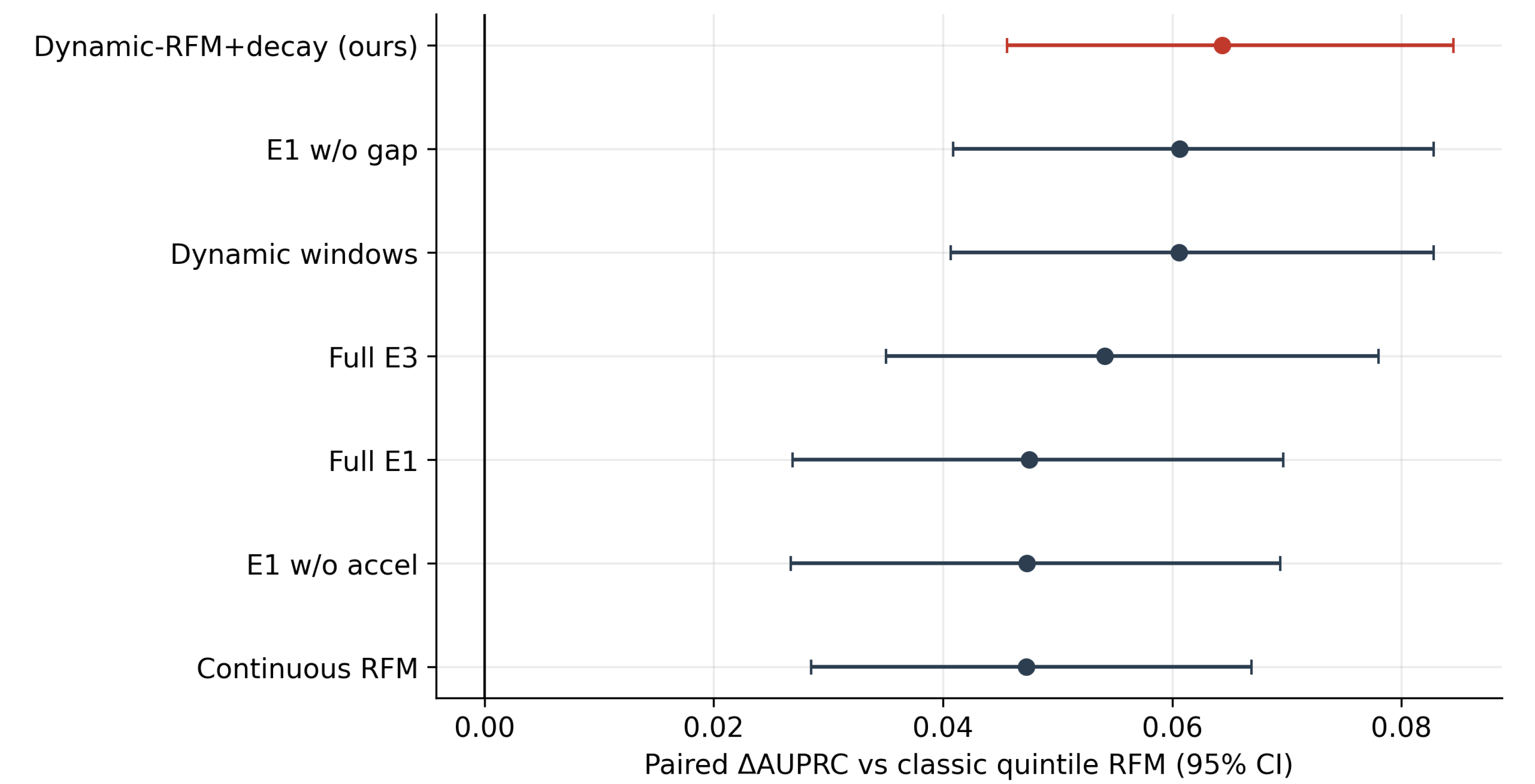
This study presents DynRFM-Hazard, a transparent framework for prioritizing manual review of historical customers at a medical-aesthetic institution. Continuous RFM values and seven exponentially decayed category-specific purchase-memory variables define a ten-variable customer state. Three regularized logistic models estimate first positive-payment probabilities in days 0-30, 31-90, and 91-180, and their survival-product combination yields internally consistent cumulative probabilities. Chronologically separated data included 67,106 item-level records from 9,412 customers. In the chronologically separated evaluation with a 23 July 2024 cutoff, the ten-variable representation, selected by validation AUPRC only, achieved AUROC 0.7999, AUPRC 0.3230, Brier score 0.0846, ECE 0.0585, and Top-10% precision 0.3667. It exceeded classical quintile RFM by 0.0644 AUPRC (1,000 customer-level paired bootstrap draws; 95% CI: 0.0460-0.0849). A cutoff-safe histogram-gradient tree achieved AUPRC 0.3231; the DynRFM-minus-tree difference was -0.0001 (95% CI: -0.0176-0.0169), so the data did not distinguish their ranking performance. A complementary retrospective rolling assessment at six earlier, fully mature time origins found mean AUPRC 0.4276 for the fixed ten-variable model versus 0.3516 for quintile RFM; the customer-clustered macro-origin difference was 0.0760 (95% CI: 0.0653-0.0875). This analysis reuses the same authorized dataset and cannot replace independent validation on newly collected or external data. Later-window probabilities were optimistic at the high end, so the framework supports relative manual-review ranking rather than fixed-threshold decisions. It is not a causal marketing, automatic-contact, or clinical-recommendation system.
Keywords:
dynamic RFM
; discrete-interval hazard
; repurchase prediction
; manual review ranking
; probability calibration
; artificial intelligence
1. Introduction
The operational question addressed in this paper is narrow but important: at a particular date, which historical customers should be reviewed first when staff time is limited? It is not a question of assigning a permanent “high-value customer” label. A customer who spent heavily in the past may have made no recent payment, while another customer with a lower lifetime total may be actively returning. The two customers should not receive the same priority merely because their past totals are similar.
This distinction is especially relevant in medical-aesthetic services. Payment patterns can reflect price, treatment cycle, season, promotions, appointment availability, and individual choice. The available data usually do not explain these mechanisms. A model built from payment events can estimate the probability of a future positive payment under observed history. It cannot determine whether a campaign caused the payment, whether a person should receive a treatment, or whether a customer should be contacted automatically.
Limited review capacity makes ranking more useful than a single average accuracy score. A useful model should place more eventual repurchasers near the top of a fixed-size review list. At the same time, a ranking model should not be described as if every high-scoring person will repurchase. We therefore report ranking, probability quality, and list efficiency separately.
DynRFM-Hazard was designed for this practical boundary. It uses continuous RFM values rather than coarse quintiles, keeps recent category-specific purchase signals through exponential decay, and models several future horizons in their natural order. The contribution is not a new logistic link function. The contribution is a reproducible combination of customer-state representation, time-isolated labels, interval-specific estimation, validation-only probability adjustment, and transparent list-based evaluation.
The study makes three applied contributions. First, it compresses continuous purchase history and category-specific timing into a ten-variable state that can be recalculated and audited at any cutoff. Second, it connects label maturity, chronological separation, interval probabilities, and validation-only adjustment in one reproducible protocol. Third, it evaluates eight predefined representations, a nonlinear tree baseline, fixed-capacity review lists, calibration drift, and negative upgrade results under the same customer and time rules. These contributions target reliable implementation under limited operational data rather than algorithmic novelty in isolation.
Figure 1.
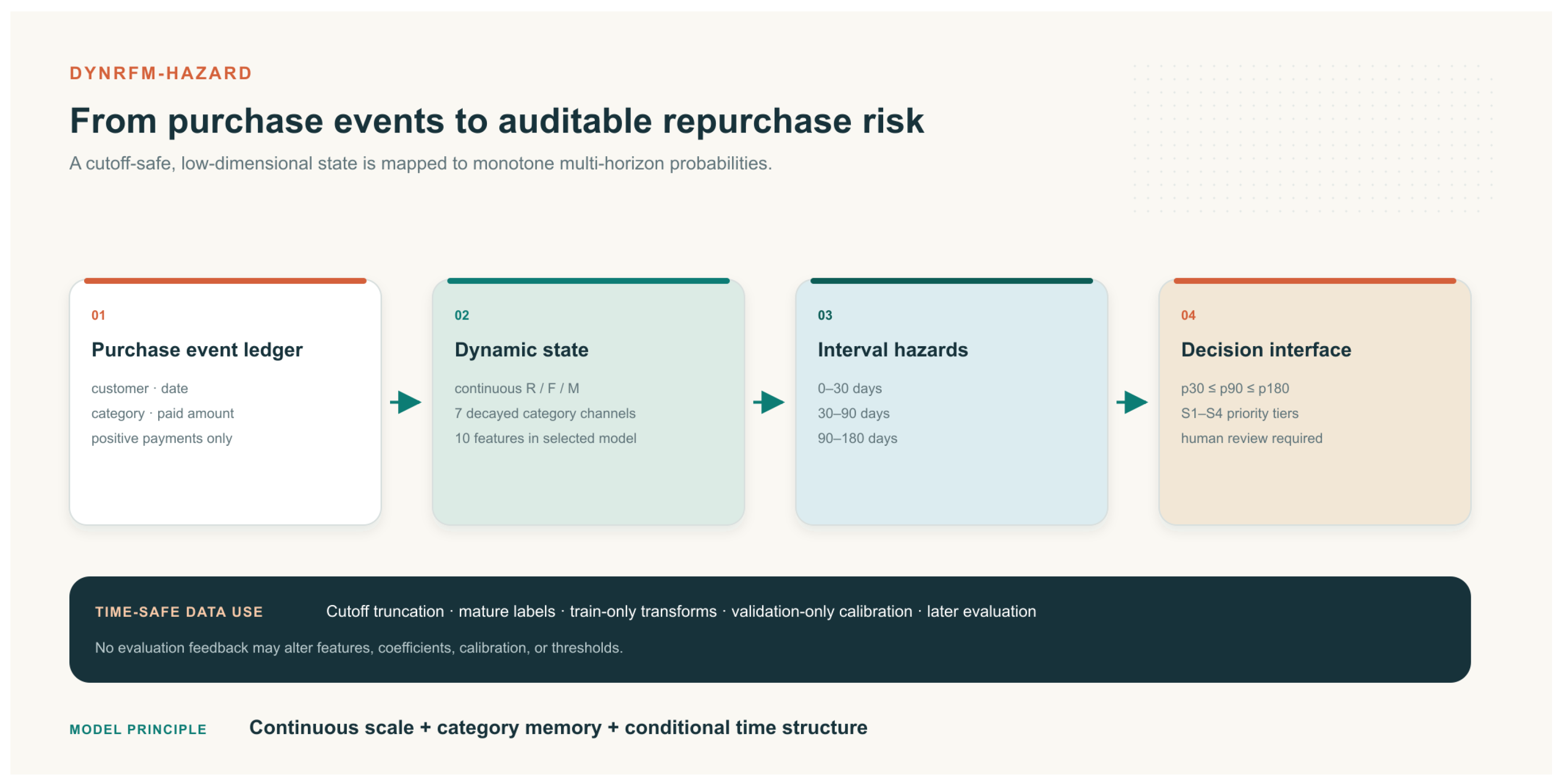
DynRFM-Hazard overview. The dark band marks time isolation among data, features, estimation, and decision support.
Figure 1.
DynRFM-Hazard overview. The dark band marks time isolation among data, features, estimation, and decision support.
2. Related Work and Research Positioning
2.1. From RFM Segmentation to Predictive Inputs
RFM summarizes customer history through recency, frequency, and monetary value. It is easy to explain and has been widely used for segmentation, churn detection, and response prediction [1,2,3,4]. Yet its exact definition varies across studies. Frequency may mean orders, item rows, or distinct purchase days; monetary value may mean gross amount, net payment, or spending in a specific observation window. We define frequency as the number of distinct positive-payment dates, monetary value as positive payments before the cutoff date, and recency against the same cutoff date for every customer.
Classical quintile RFM is useful for human-readable segments but discards differences inside each bin. The distance between a payment seven days ago and a payment 29 days ago disappears when both are assigned to the same group. Continuous RFM retains this information. In a ranking application, score direction, ordering, and textual explanation must also remain consistent, otherwise the same feature may be interpreted in opposite business directions [5].
2.2. Dynamic Customer State and Maintainable Representation
Time-varying RFM, dynamic features, and sequence models have shown that recent and remote behavior should not receive identical weight [6,7,8,9]. Full sequence models can represent complex paths, but they require more data, tuning, monitoring, and maintenance. DynRFM-Hazard uses a deliberately smaller representation. For each of seven stable payment categories, a past event loses half of its weight every 90 days. The representation therefore retains category, repetition, and timing without creating hundreds of sparse item-name columns.
This choice is an engineering decision, not a claim that exponential decay is a clinical process. Work on resource-constrained deployment, functional-relationship modeling, and concept quantification likewise shows the value of keeping testable domain structure while controlling maintenance cost [10,11,12]. The question tested here is whether this compact representation improves future ranking, not whether it reconstructs every purchase sequence.
2.3. Multiple Time Horizons and Probability Quality
Separate binary models for 30, 90, and 180 days can give an illogical result: a shorter-horizon probability may exceed a longer-horizon probability. Discrete-interval event models avoid this inconsistency by estimating the first-payment probability only among customers who have not repurchased in earlier intervals [13,14]. The cumulative probabilities are then computed from the product of interval survival probabilities.
When repurchasers are relatively uncommon, accuracy is misleading. In this study, predicting no repurchase for everyone would exceed 90% accuracy but would produce no useful list. AUPRC and precision-recall curves are more informative for this use case [15,16]. Ranking must still be separated from probability calibration. Brier score, expected calibration error, and reliability plots test whether predicted probabilities agree with observed frequencies [17,18]. A probability score has decision value only when it is placed in a clear, documented review workflow [19].
2.4. Positioning of the Present Study
Medical-aesthetic studies often discuss service fairness, experience, trust, engagement, and repurchase intention [20]. These factors are important, but intention is not the same as a recorded positive payment. The present study uses a payment event because it is auditable in the available operational data. We do not claim that payment events reveal treatment need, clinical suitability, or marketing response.
Recent churn and repurchase studies have examined ensemble learning and performance frameworks under different service datasets [21,22,23]. A second group combines RFM with clustering, deep networks, support vector machines, self-organizing maps, association rules, or discount information [24,25,26,27,28,29]. These studies show that RFM can support richer predictive systems, but an observed gain may come from the representation, the estimator, or both. The main feature comparison in this study therefore holds the estimator and customer pool constant.
Other studies compare ensemble deep learning, conventional machine learning, feature reduction, and multiple neural architectures [30,31,32,33,34]. Their results support empirical comparison rather than a universal algorithm ranking. Event rates, eligibility rules, observation windows, and the definition of frequency differ across datasets. Accordingly, scores reported in other studies are not treated as external benchmarks for the numerical results in this paper.
The research position is therefore specific. DynRFM-Hazard is a low-dimensional dynamic customer-state model. It uses chronological separation, mature labels, fixed feature definitions, and validation-only probability adjustment. Its operational endpoint is manual review ranking. It does not identify causal uplift, provide clinical advice, or claim that its parameters transfer unchanged to another institution.
3. Materials and Methods
3.1. Data Source, Privacy Protection, and Time Isolation
The data were supplied by a medical-aesthetic institution as part of a commissioned collaborative research project. The institution authorized the use of fully de-identified and anonymized purchase-event data for this study. Before analysis, names, customer numbers, contact details, identity-document numbers, and detailed organizational fields were removed. The working data retained only fields needed for modeling. To protect commercial confidentiality, the institution is not identified by name.
The source contained 67,106 item-level records, 9,412 customers, and 692 item names. A customer state was rebuilt at each predefined cutoff date. Events after the cutoff were excluded before any feature was calculated. A positive payment after the cutoff defined repurchase. A 90-day negative label was used only if the full 90-day observation period was available. Customers whose outcome was not yet observable were not treated as non-repurchasers.

Table 1.
Chronological roles, cutoff dates, eligible customers, and observed repurchase rates.
| Window | Cutoff date | Eligible customers | 30-day repurchase | 90-day repurchase | 180-day repurchase |
|---|---|---|---|---|---|
| Training 1 | 2022-10-23 | 2,299 | 17.27% | 22.58% | 34.75% |
| Training 2 | 2023-01-23 | 3,381 | 5.94% | 23.01% | 29.99% |
| Training 3 | 2023-04-23 | 4,839 | 6.90% | 15.33% | 24.41% |
| Training 4 | 2023-07-23 | 5,606 | 5.33% | 15.09% | 28.79% |
| Validation | 2024-01-23 | 7,510 | 6.15% | 17.02% | 24.73% |
| Evaluation | 2024-07-23 | 9,080 | 4.16% | 9.71% | Not mature |
The extract ends on 23 October 2024. It therefore cannot supply a later 90-day outcome window after the July 2024 assessment. To test whether the fixed ten-variable representation behaves consistently across earlier operating periods, we also performed a retrospective rolling temporal assessment. It contains six assessment origins from November 2023 to April 2024. For each origin, all training cutoffs precede a validation cutoff, and the validation cutoff precedes the assessment cutoff by more than 180 days. This buffer permits mature labels for all three interval models. The ten-variable DynRFM representation was evaluated as a fixed design. In-fold validation selection was retained only as a stability diagnostic; it did not use the assessment labels.
3.2. Dynamic RFM Representation
For customer u at cutoff t0, recency is the number of days since the latest positive payment, frequency is the number of distinct positive-payment dates, and monetary value is the cumulative positive amount. Several item rows on the same payment date increase monetary value but count once for frequency. If a customer has history but no positive payment, frequency and monetary value are zero; recency is the number of days from the first historical event to the cutoff. This prevents “no positive payment” from being interpreted as “paid today”.
For category c, the decayed purchase-memory feature is
The final DynRFM state is ten-dimensional: continuous RFM plus seven decayed category variables. Means, standard deviations, category mapping, and column order are derived from training data only and reused in validation, evaluation, and future scoring.
3.3. Discrete-Interval Hazard Model
The model uses three intervals: days 0-30, 31-90, and 91-180. A customer contributes to an interval only when the customer has not repurchased earlier and the interval outcome is fully observed. For interval k, a regularized logistic model estimates conditional first-payment probability:
The cumulative probability through each target horizon is computed as
This construction guarantees that the 30-day probability does not exceed the 90-day probability and that the 90-day probability does not exceed the 180-day probability. A validation-window adjustment can shift interval probabilities without changing customer order. It is intended to address an overall probability shift, not to repair a poor ranking relationship.
Figure 2.
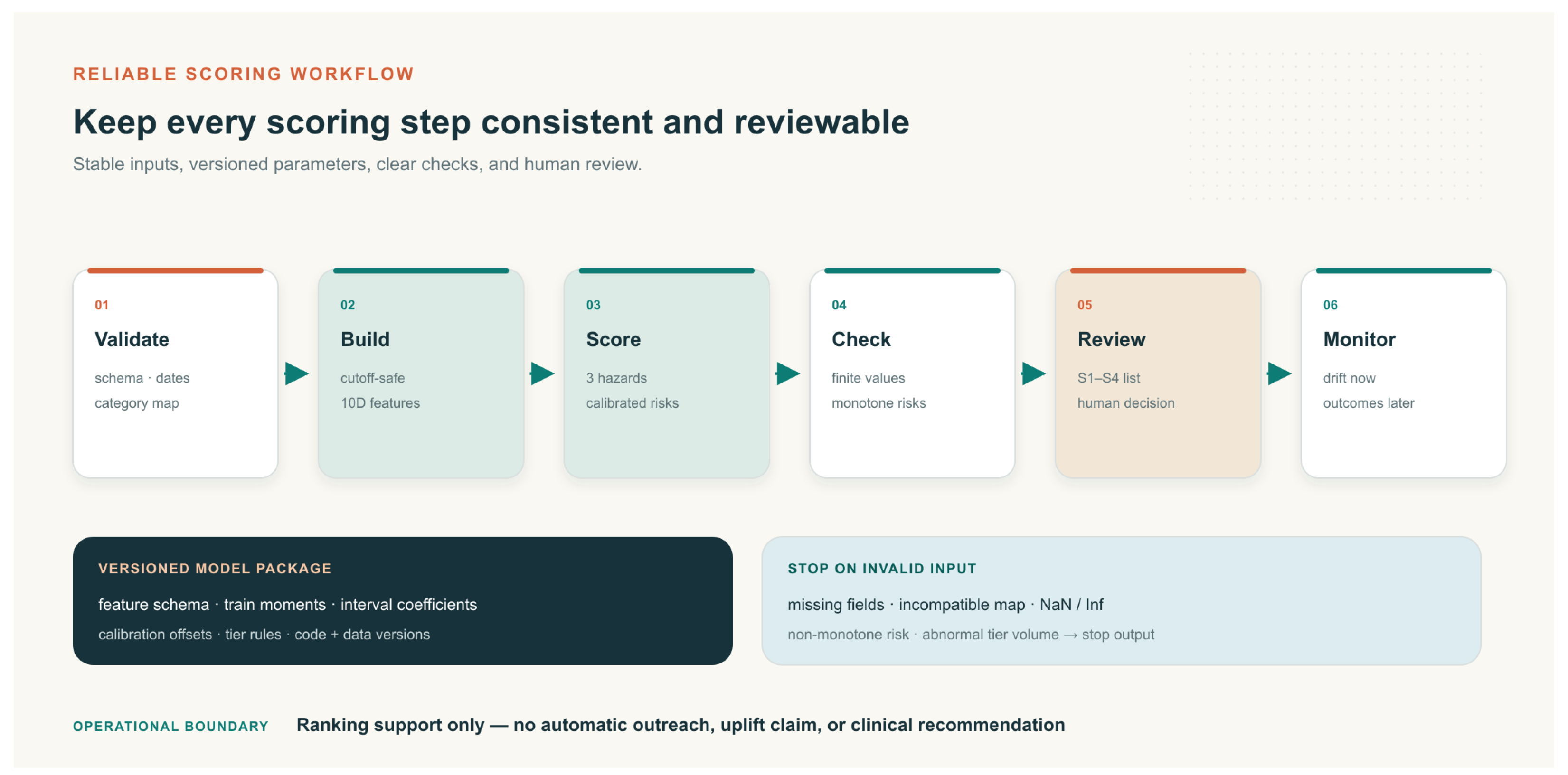
Reproducible scoring workflow. The process checks input data, builds features, calculates probabilities, validates outputs, and routes the list to human review. Scoring stops when a required check fails.
Figure 2.
Reproducible scoring workflow. The process checks input data, builds features, calculates probabilities, validates outputs, and routes the list to human review. Scoring stops when a required check fails.
3.4. Comparison and Evaluation
Eight predefined feature representations were compared with the same logistic estimator, regularization, customer pool, and time rules. Validation AUPRC selected the configuration, using fewer features and then the model name as predetermined tie rules. Assessment labels were not available to this selection step. Classical quintile RFM, continuous RFM, the predefined Dynamic-RFM representations, and a histogram-gradient tree using the same cutoff-safe derived fields were reported under the same customer pool and target definition. Metrics include AUROC, AUPRC, Brier score, ten-bin ECE, reliability plots, and Top 5%, 10%, 20%, and 30% precision, recall, and lift. The main later-window comparison uses 1,000 paired customer-level bootstrap draws. For the six-origin retrospective assessment, the same fixed DynRFM representation is compared with quintile RFM at each origin. A second 1,000-draw bootstrap resamples customers as clusters across repeated origins and averages the within-origin AUPRC difference. This accounts for recurring customers without claiming that the six overlapping historical periods are independent studies. A new authorized future window or another institution is still required for independent validation.
3.5. Decision Target and Unit of Analysis
The study begins with a precise prediction target. One observation is not an item row and not a permanent customer profile. It is a customer state reconstructed at a specified cutoff date. The state includes only payment events that were available on that date. The target asks whether the customer makes a first positive payment after the cutoff and within a stated horizon. This definition prevents several common substitutions. A completed service is not automatically a payment event. An appointment is not a payment event. A consultation is not a payment event. A cancelled appointment is not a negative payment outcome. The model therefore makes no attempt to infer a full care journey from an incomplete ledger.
This unit of analysis also makes the model usable in a periodic workflow. At the start of a scoring cycle, the institution chooses a cutoff date and creates one state per eligible historical customer. The scoring service does not need to guess how long a customer has been inactive from a dashboard snapshot. It rebuilds recency, frequency, monetary value, and category memories from dated events. The same definition is applied in the evaluation and in any future authorized scoring run. A customer may appear at more than one historical cutoff during training, because the customer state changes over time. The evaluation window contains one state per eligible customer. This difference is intentional: repeated historical states train a time-aware relationship, while the evaluation list represents one operational decision date.
The target is deliberately narrower than customer value. A customer can have a high probability of another small payment and a lower probability of a large payment. The present model estimates only the first part. It does not multiply probability by expected amount, and it does not rank customers by lifetime revenue. That choice keeps the evidence aligned with the available data. A value model would require an additional, separately validated amount model and a clear treatment of refunds, packages, price changes, and deferred revenue. None of those assumptions is needed to answer the practical question of which existing records deserve manual review first.
3.6. Event Rules and Reproducible State Construction
The apparently simple phrase “purchase history” hides several implementation decisions. DynRFM-Hazard counts a positive payment day rather than a line count when it constructs frequency. A customer can purchase more than one item on a single date. Those items contribute their paid amounts to monetary value, but they describe one active date rather than several separate return visits. Without this rule, item bundles would artificially increase frequency and make a transaction format look like customer loyalty. The rule is easy to test because a duplicated same-day item should alter the amount input but not the frequency input.
Recency has an equally important boundary. It is the elapsed number of days between the cutoff and the most recent positive payment. Customers with recorded history but no positive payment are not treated as if they paid on the cutoff. Their frequency and monetary values are zero, and their recency is measured from the first available historical event. This representation is not a claim that their future behavior is identical. It simply prevents a missing positive payment from being encoded as maximum recency strength. Every implementation should retain this distinction in its data contract and test suite.
The category dictionary is a second reproducibility device. The raw data contain 692 item names. Item names can be renamed, discontinued, or introduced after an evaluation starts. A direct one-hot representation would create a large sparse matrix and make future scoring sensitive to new labels. The study therefore maps authorized names into seven broad payment categories before model fitting. The mapping is fixed for a run. A new raw label is reported as a mapping problem rather than quietly creating a new feature. This is a small operational safeguard, but it is essential for interpreting a feature vector in the same way across time.
3.7. Compact Feature Design
The ten-variable state does not attempt to memorise every sequence of purchases. Its three continuous RFM values summarize overall recency, repeat activity, and accumulated positive payments. Its seven decay variables retain a separate short memory for each approved category. The combination answers a useful middle-level question: has this customer shown a recent and repeated payment pattern in one or more stable categories? It does not try to infer the reason for that pattern. It also does not treat category membership as a clinical label.
Exponential decay has a direct operational meaning. With a 90-day half-life, an event that occurred 90 days before the cutoff contributes one half of the weight of an otherwise identical event on the cutoff. At 180 days it contributes one quarter. Repeated recent payments accumulate. This mechanism gives the representation a controlled way to distinguish a recently repeated category from a historically important but distant category. The half-life is a modeling convention aligned with the primary 90-day horizon. It is not an estimate of a biological treatment cycle, and it should be reconsidered only in a new time-separated evaluation.
The comparison results explain why compactness was retained. Continuous RFM already removes much of the information loss introduced by quintile bins. Dynamic windows and category decay add useful timing information. Wider representations add acceleration, gap, and related variables derived from the same small set of event dates. Such variables can be informative in another dataset, but they can also repeat the same signal with different scales. The ten-variable representation is therefore not presented as universally optimal. It is the most interpretable representation among the evaluated alternatives for the stated population and practical objective.
3.8. Ordered Interval Probabilities
The interval design protects a basic property that separate classifiers may violate. A person who has a 30-day probability of first payment also has a 90-day opportunity to make that payment. The 90-day cumulative probability should therefore never be lower than the 30-day cumulative probability. DynRFM-Hazard estimates conditional first-payment probability in successive intervals and then combines the results through survival multiplication. If the interval probabilities are h1, h2, and h3, the 90-day result is one minus the probability of no event in the first two intervals. The 180-day result adds the third interval in the same way.
This construction is easy to audit and explain. The first model asks about payment in days 0-30. The second is evaluated only for customers who have not already made a positive payment in that first interval. The third follows the same logic for days 91-180. A customer without a complete observation period does not create a negative label for a later interval. The customer is simply not evaluated for that interval. This rule avoids treating administrative truncation as evidence of non-repurchase.
Regularized logistic regression was selected for the interval models because it provides a stable, inspectable baseline for a low-dimensional representation. The L2 penalty coefficient was fixed at for every feature representation and interval comparison. L2 regularization limits extremely large weights when correlated inputs are present. It does not turn a linear model into a causal model, and it does not make omitted operational variables disappear. Its advantage here is transparency: the input columns, scaling statistics, coefficients, and calibration adjustments can all be recorded in a manifest. More complex models should be compared only when they receive exactly the same cutoff-limited inputs and the same label-maturity treatment.
3.9. Separation of Learning, Adjustment, and Evaluation
The evaluation uses time separation because random row splitting would mix earlier and later payment conditions. Training snapshots come from earlier cutoffs. A later cutoff is used to adjust the overall probability level. A still later cutoff is used to examine the predefined representations under a different observed payment rate. The order matters. Information from a later period cannot improve a feature, a scaling statistic, or a probability adjustment for an earlier decision date.
Three layers must be kept distinct. First, representation learning decides which fields are included and how they are transformed. Second, probability adjustment aligns interval outputs to the validation distribution without changing their order. Third, evaluation describes how a predefined representation behaves in the later assessment window. Combining these roles makes a result difficult to interpret. For example, recalibrating on the evaluation labels could reduce an apparent probability error while hiding the fact that a later period had a different repurchase rate. Conversely, using the evaluation AUPRC to choose among many representations would make the reported winner partly a consequence of that evaluation population.
The accompanying protocol and software make these boundaries explicit. The protocol specifies the target, the approved fields, same-day aggregation, category mapping, label maturity, and permitted decision output. The selection gate rejects final-window labels when it chooses a configuration from validation results. A redacted manifest records the feature order, category mapping, scaling summary, random seed, and input checksum without disclosing a customer record. These controls do not create performance. They make it possible to determine which performance statement the evidence actually supports.
3.10. Evaluation Metrics and Decision-List Measures
No single metric answers every operational question. AUROC measures whether a positive-payment case tends to receive a higher score than a non-case across the full ranked population. It remains useful as a broad discrimination summary, but it gives equal attention to portions of the list that a small review team may never reach. AUPRC is more sensitive to the positive-payment class when that class is uncommon. It answers whether precision remains useful as recall grows. This is why AUPRC is the principal representation-comparison measure in this work [15,16].
Top-fraction precision, recall, and lift translate that evidence into review capacity. Precision describes the positive-payment proportion inside a selected list. Recall describes how many of all eventual positive-payment cases appear in that list. Lift divides list precision by the overall repurchase rate. It is a concentration ratio, not an expected revenue multiplier and not a marketing effect. A Top-10% lift of 3.776 means that the selected list contains positive-payment cases at 3.776 times the overall observed rate in the same population. It says nothing about what would happen if the customers were contacted.
Brier score, expected calibration error, calibration intercept, calibration slope, and reliability plots answer a different question: whether stated probabilities resemble observed frequencies. The later-window evaluation shows that a representation can rank well while its larger predicted probabilities are optimistic in a later period. This is not a contradiction. A monotonic transformation can preserve a ranking and alter probability accuracy. The reporting structure therefore avoids a vague claim that one model is simply “better.” It distinguishes list ordering from absolute probability use and gives the two tasks separate evidence.
4. Results
4.1. Data Profile and Model Comparison
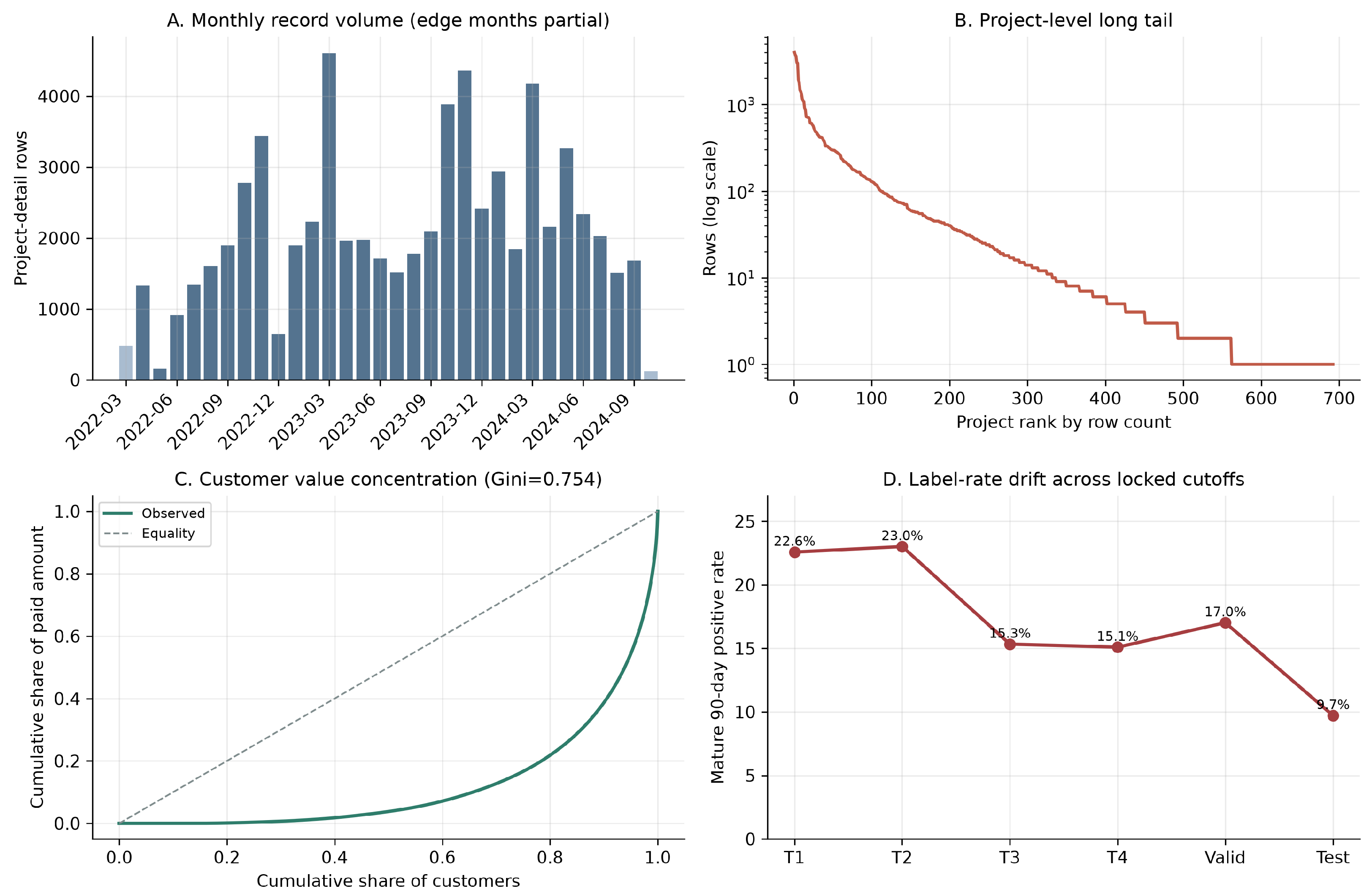
Among 9,412 customers, 8,060 had at least one positive payment and 4,052 had at least two distinct positive-payment dates. The median interval between positive-payment dates was 72 days. Item names were long-tailed: 131 appeared once and 267 appeared fewer than five times. Seven broad payment categories therefore provided a more stable representation than 692 item-name indicators.
Figure 3.
Data size and time variation. Monthly record count varies, item names are long-tailed, spending is concentrated, and 90-day repurchase rate changes across cutoff dates.
Figure 3.
Data size and time variation. Monthly record count varies, item names are long-tailed, spending is concentrated, and 90-day repurchase rate changes across cutoff dates.
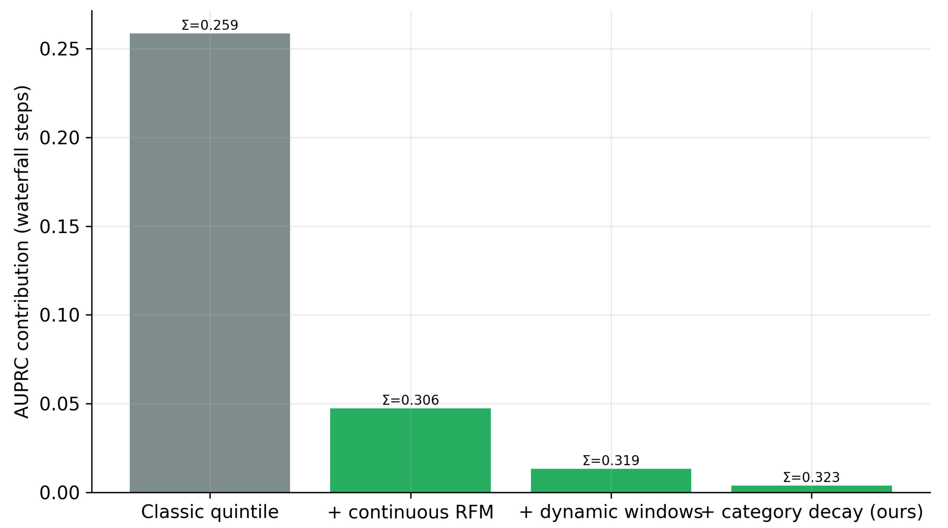
The 10-variable continuous-RFM-plus-decay representation had the highest validation AUPRC (0.4513) among the predefined logistic representations and was therefore selected before evaluation labels were used. In the evaluation window, it improved AUPRC by 0.0644 over classical quintile RFM. Larger candidate representations did not show a reliable additional advantage.
Table 2.
Later-window performance of the eight predefined logistic feature representations.
| Feature representation | Dimensions | AUROC | AUPRC | Brier | ECE | Precision at Top 10% |
|---|---|---|---|---|---|---|
| Classical quintile RFM | 3 | 0.7898 | 0.2585 | 0.0824 | 0.0609 | 0.3282 |
| Continuous RFM | 3 | 0.7931 | 0.3058 | 0.0889 | 0.0644 | 0.3601 |
| Dynamic windows | 16 | 0.7959 | 0.3195 | 0.0818 | 0.0538 | 0.3568 |
| E1 without acceleration | 19 | 0.7888 | 0.3070 | 0.0820 | 0.0514 | 0.3425 |
| E1 without gap variables | 18 | 0.7959 | 0.3194 | 0.0818 | 0.0538 | 0.3568 |
| Full E1 | 21 | 0.7888 | 0.3070 | 0.0820 | 0.0514 | 0.3425 |
| DynRFM-Hazard (validation-selected) | 10 | 0.7999 | 0.3230 | 0.0846 | 0.0585 | 0.3667 |
| Full E3 | 28 | 0.7913 | 0.3144 | 0.0810 | 0.0490 | 0.3447 |
The cutoff-safe histogram-gradient tree achieved AUPRC 0.3231, AUROC 0.8042, Brier score 0.0800, ECE 0.0575, and Top-10% precision 0.3634. Its AUPRC was 0.0001 higher than the selected DynRFM-Hazard representation; the paired 1,000-draw interval for the DynRFM-minus-tree difference was -0.0176 to 0.0169. The evaluation therefore does not establish a ranking difference between the compact representation and this stronger nonlinear baseline. The reason to retain the compact representation is not higher predictive performance. It is the ability to use ten transparent inputs and a small, auditable scoring component when those are operational requirements.
Figure 4.
Validation-only representation selection, later-window benchmark comparison, and 1,000-draw customer-level precision intervals for fixed manual-review list sizes.
Figure 4.
Validation-only representation selection, later-window benchmark comparison, and 1,000-draw customer-level precision intervals for fixed manual-review list sizes.
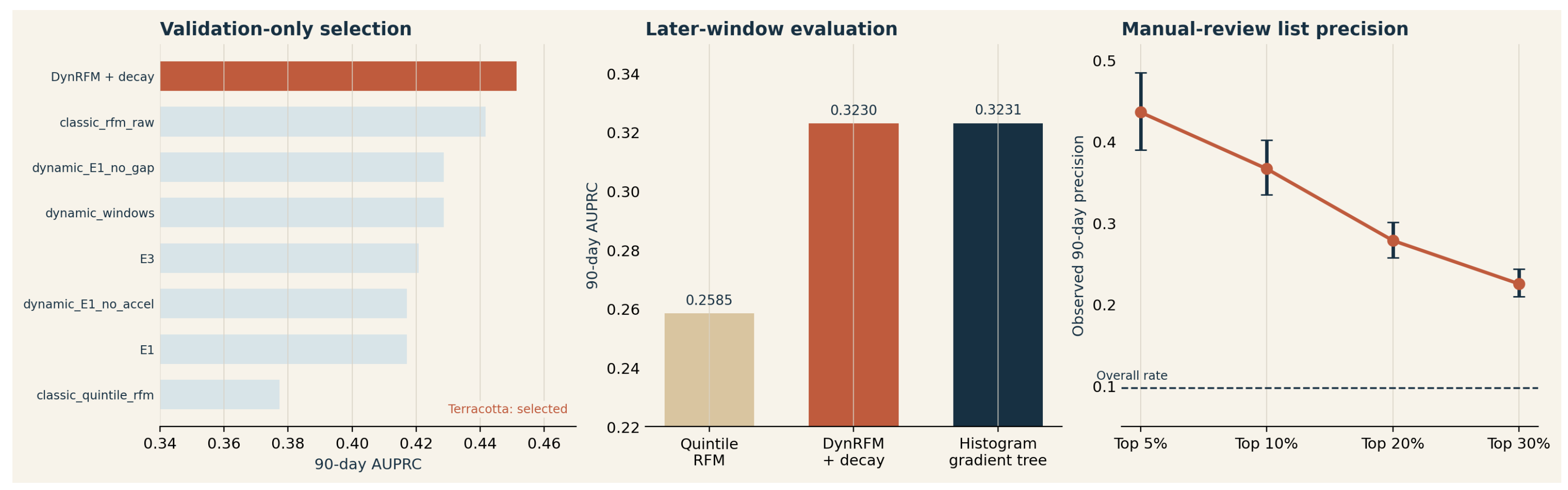
Figure 5.
Ninety-day AUPRC for predefined feature representations in the chronologically separated evaluation. The terracotta marker indicates the ten-variable representation.
Figure 5.
Ninety-day AUPRC for predefined feature representations in the chronologically separated evaluation. The terracotta marker indicates the ten-variable representation.
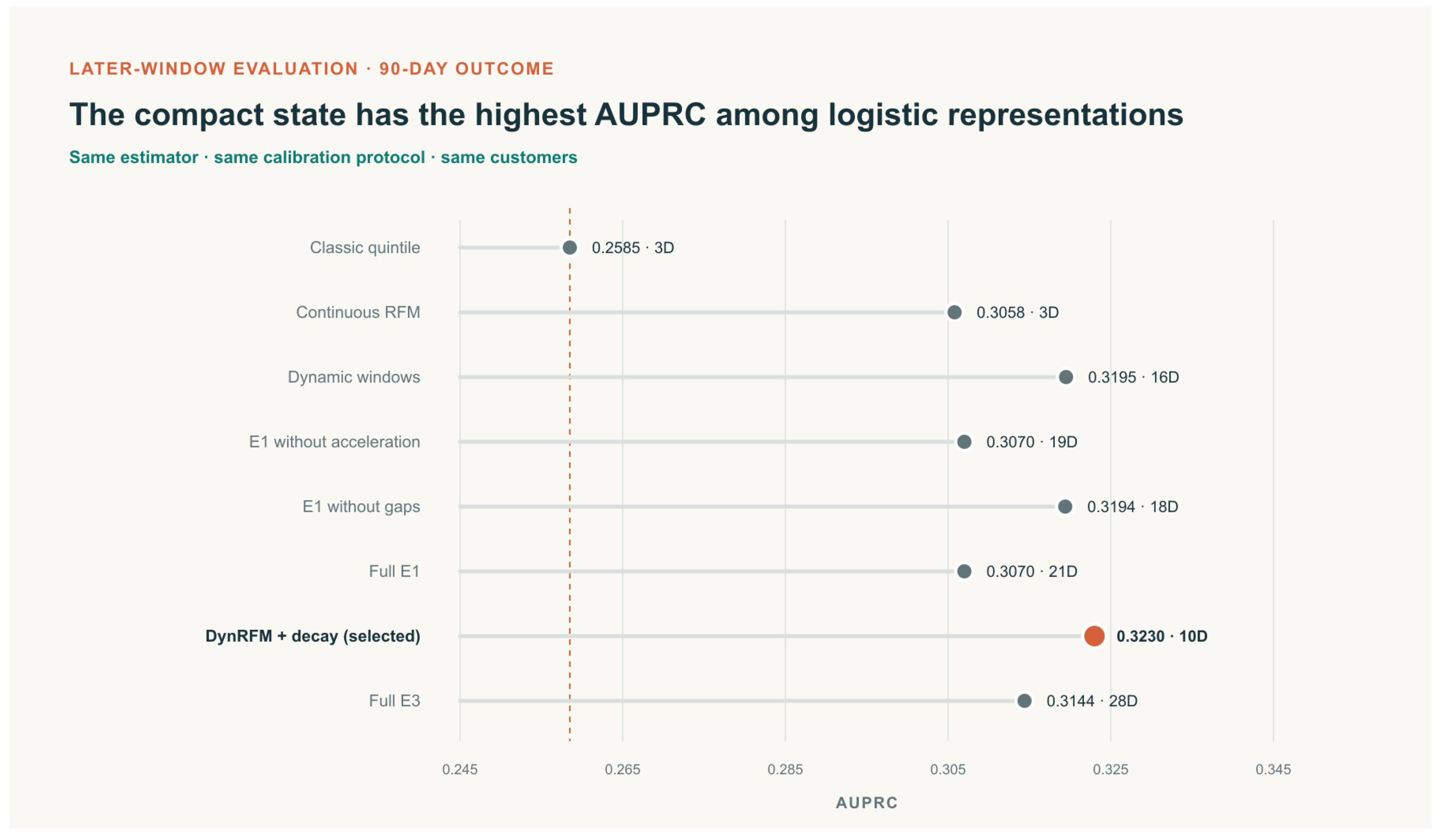
Figure 6.
Paired AUPRC gain over classical quintile RFM. The ten-variable representation has the largest point estimate; the intervals quantify sampling uncertainty in the evaluation population.
Figure 6.
Paired AUPRC gain over classical quintile RFM. The ten-variable representation has the largest point estimate; the intervals quantify sampling uncertainty in the evaluation population.
4.2. List Efficiency and Calibration
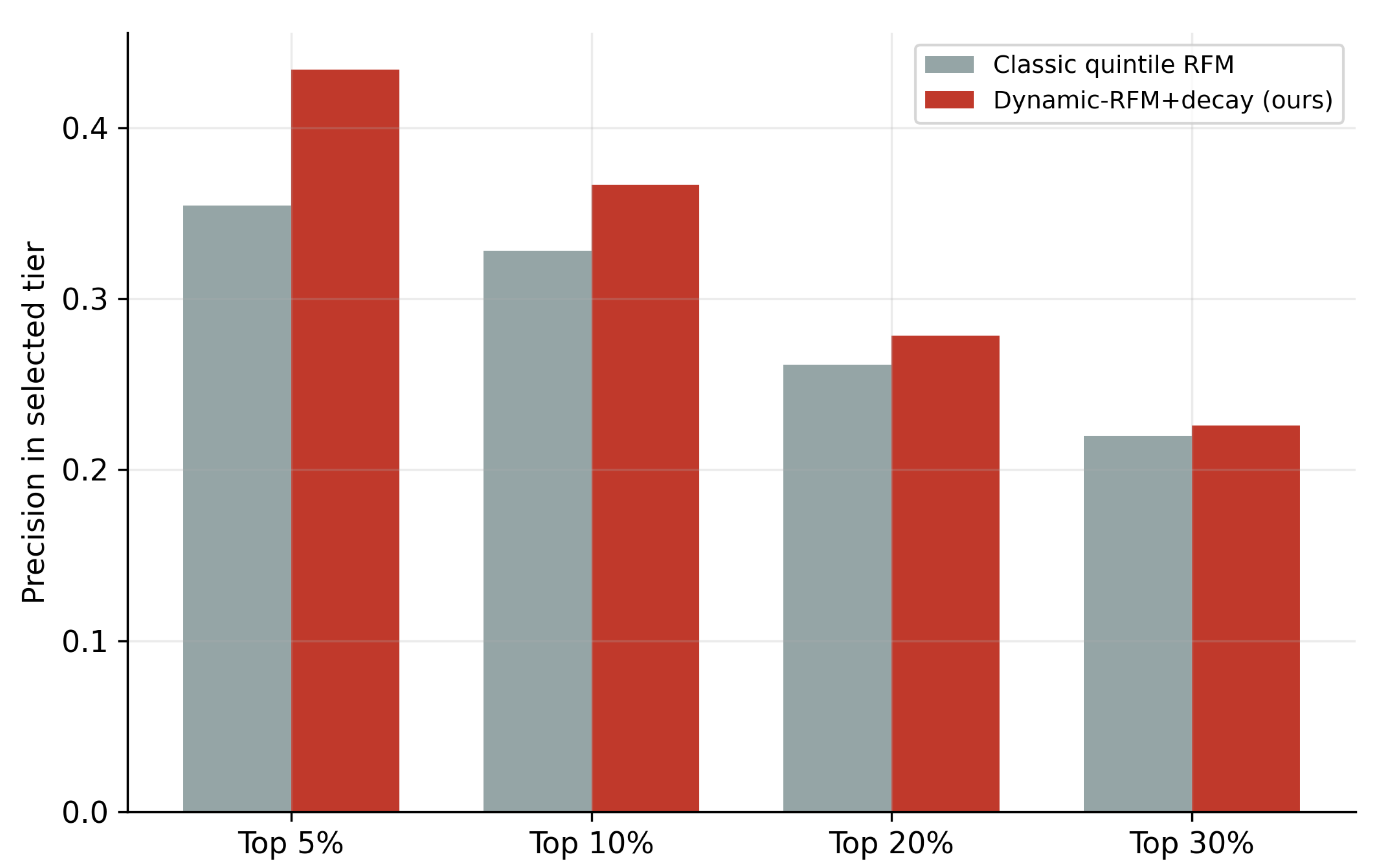
In the 90-day evaluation window, the Top-10% list contained 908 customers and approximately 333 repurchasers. Precision was 0.3667, recall was 0.3776, and lift was 3.776 relative to the overall 9.71% repurchase rate. A smaller Top-5% list improved precision to 0.4361 but covered 22.45% of eventual repurchasers. These numbers describe concentration in a review list; they do not measure revenue gain or the effect of contacting a customer.
Table 3.
Observed 90-day performance at four manual-review list sizes.
| List size | Customers | Precision | Recall | Lift |
|---|---|---|---|---|
| Top 5% | 454 | 0.4361 | 0.2245 | 4.490 |
| Top 10% | 908 | 0.3667 | 0.3776 | 3.776 |
| Top 20% | 1,816 | 0.2786 | 0.5737 | 2.868 |
| Top 30% | 2,724 | 0.2254 | 0.6961 | 2.320 |
Figure 7.
Precision-recall curves in the chronologically separated evaluation window. The dashed line is the overall 90-day repurchase rate.
Figure 7.
Precision-recall curves in the chronologically separated evaluation window. The dashed line is the overall 90-day repurchase rate.
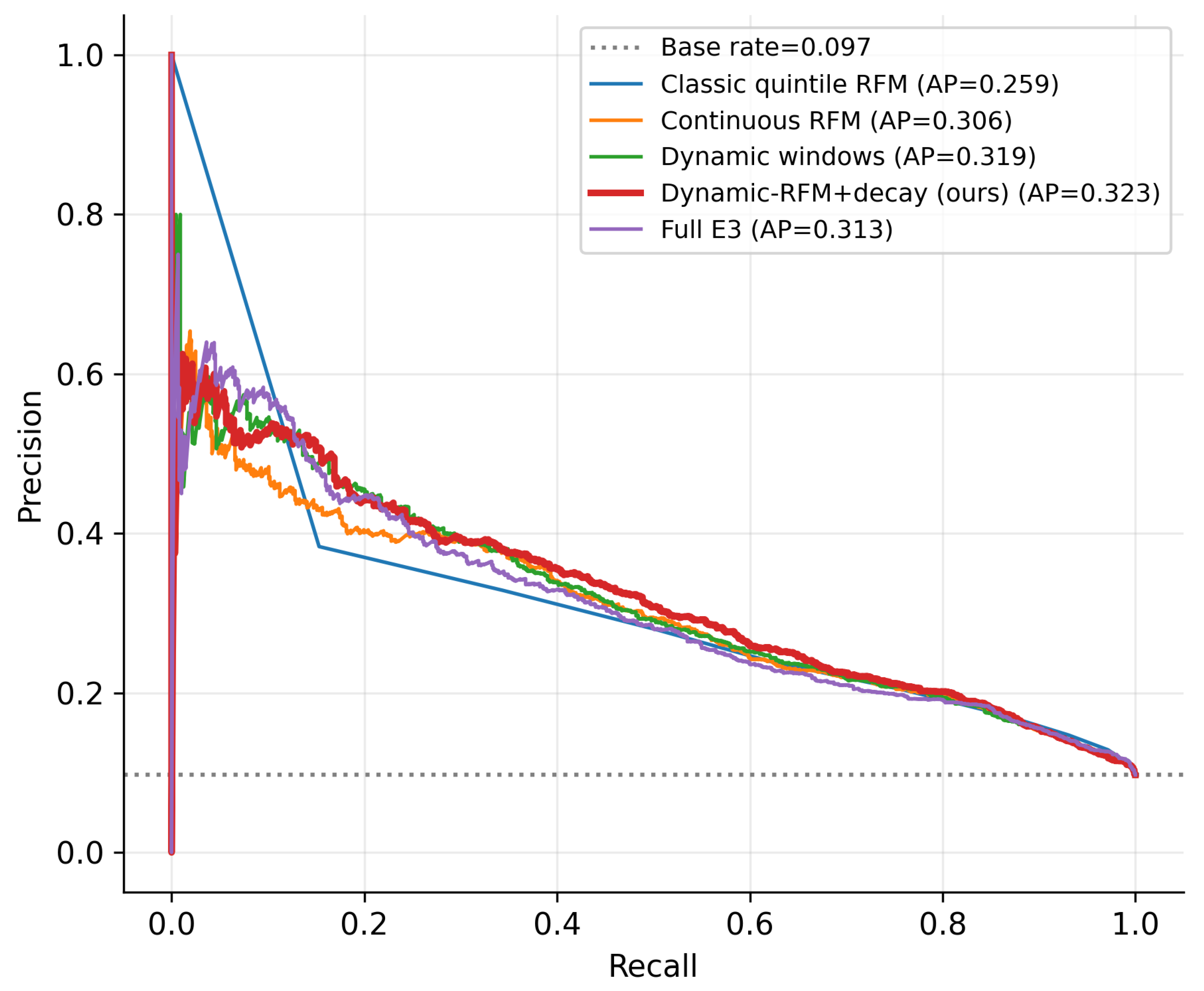
Figure 8.
Precision at several review-list sizes. DynRFM-Hazard exceeds classical quintile RFM from Top 5% to Top 30%.
Figure 8.
Precision at several review-list sizes. DynRFM-Hazard exceeds classical quintile RFM from Top 5% to Top 30%.
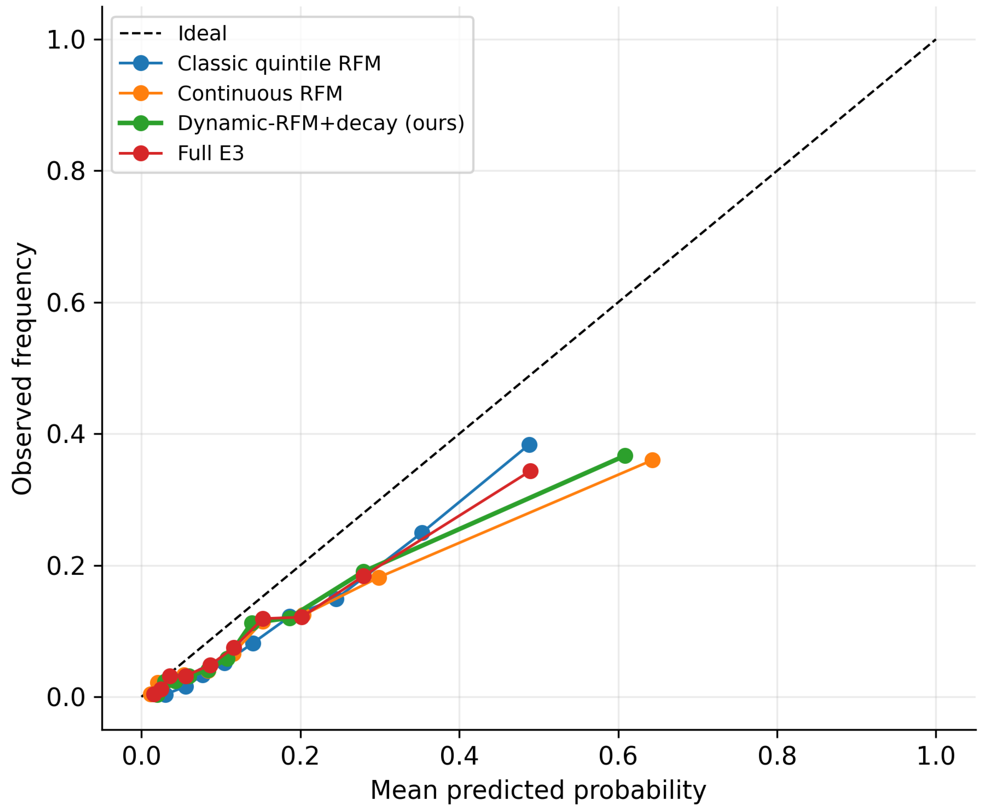
The validation 90-day rate was 17.02%, whereas the evaluation rate was 9.71%. The ten-variable representation retained useful ranking but overestimated probability in higher-score bins. This is consistent with Brier score 0.0846, ECE 0.0585, a calibration slope near 0.70, and an intercept near -1.07. The result supports relative ordering for manual review more strongly than fixed individual probability thresholds.
Figure 9.
Reliability plot for 90-day probability. The ten-variable representation ranks customers well, but its higher probability bins are systematically optimistic in the evaluation window.
Figure 9.
Reliability plot for 90-day probability. The ten-variable representation ranks customers well, but its higher probability bins are systematically optimistic in the evaluation window.
4.3. Retrospective Rolling Temporal Assessment
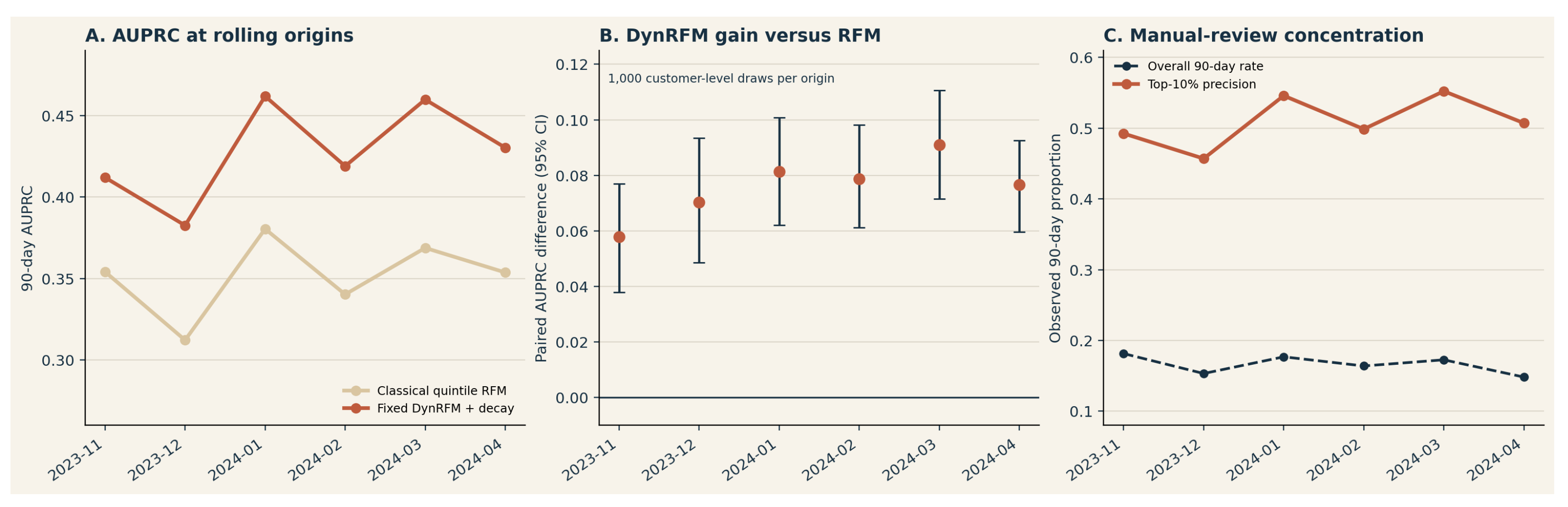
The six retrospective assessment origins covered November 2023 through April 2024. Each origin used only earlier events to fit features and coefficients, a later validation origin for probability adjustment, and a still later assessment origin for metrics. The fixed ten-variable DynRFM representation improved AUPRC over classical quintile RFM at every origin. DynRFM AUPRC ranged from 0.3826 to 0.4619 (mean 0.4276), whereas quintile RFM ranged from 0.3123 to 0.3805 (mean 0.3516). The paired AUPRC gain ranged from 0.0578 to 0.0910. Each origin-specific 95% interval excluded zero.
When repeated customer records were resampled as clusters and the within-origin differences were averaged, the macro-origin AUPRC gain was 0.0760 (95% CI: 0.0653-0.0875; 1,000 draws). Top-10% list precision ranged from 0.4570 to 0.5523, with a mean of 0.5089. The selected representation was not identical at every in-fold validation point: the ten-variable representation was selected in two origins, continuous RFM in two, and a window-based representation in two. This is useful negative evidence against a claim of universal feature superiority. It does not change the fixed-model comparison: the ten-variable representation improved over quintile RFM in all six historical assessment origins. The rolling analysis strengthens temporal robustness within this dataset, but it cannot replace independent validation on newly collected data or data from another institution.
Figure 10.
Retrospective rolling temporal assessment of the fixed ten-variable DynRFM representation. Each origin preserves chronological training, validation, and assessment roles. Error bars show 1,000 paired customer-level bootstrap intervals within each origin.
Figure 10.
Retrospective rolling temporal assessment of the fixed ten-variable DynRFM representation. Each origin preserves chronological training, validation, and assessment roles. Error bars show 1,000 paired customer-level bootstrap intervals within each origin.
4.4. Negative Results and Implementation Checks
More complex anchor-network, ORFM, and guarded-ORFM alternatives did not pass the same real-data improvement condition. Their synthetic-data behavior may still be informative, but it is not evidence for adoption in this operational setting.
Figure 11.
Negative result for the ORFM upgrade. The paired interval covers zero, so the upgrade does not meet the empirical adoption condition.
Figure 11.
Negative result for the ORFM upgrade. The paired interval covers zero, so the upgrade does not meet the empirical adoption condition.
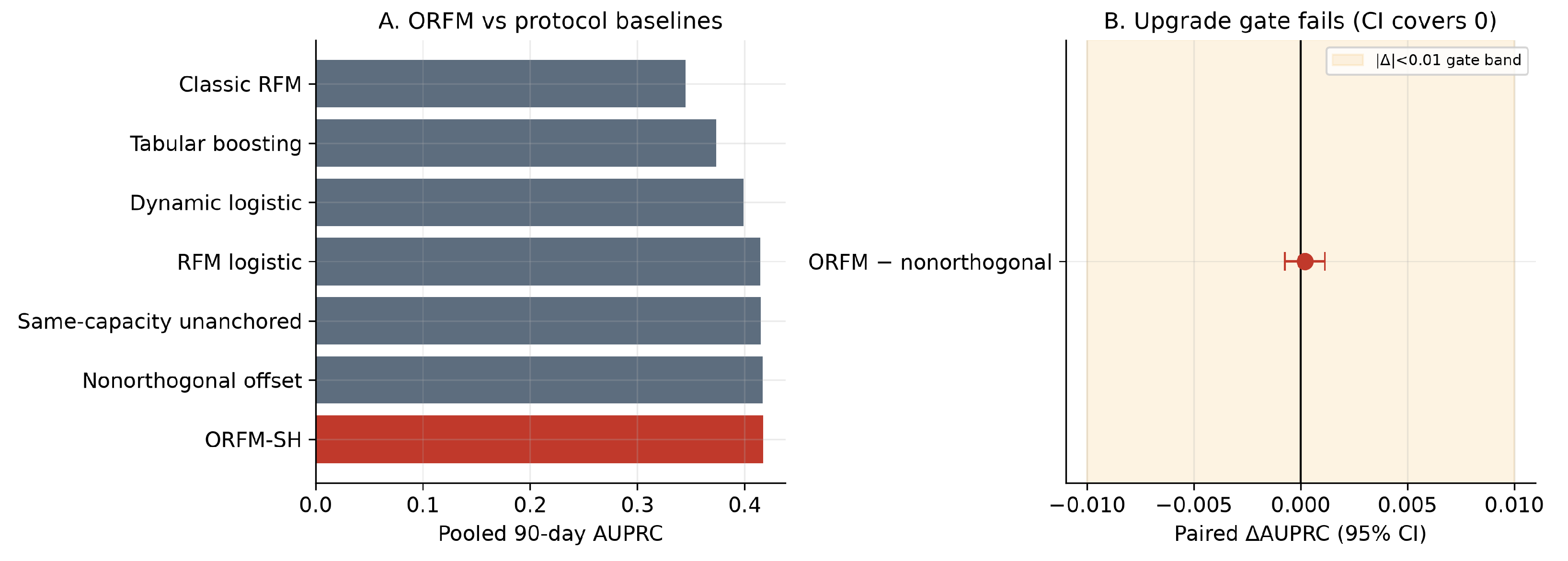
Figure 12.
AUPRC gain from classical quintile RFM to DynRFM-Hazard. Keeping continuous values provides the largest increase; dynamic windows and category decay add smaller gains.
Figure 12.
AUPRC gain from classical quintile RFM to DynRFM-Hazard. Keeping continuous values provides the largest increase; dynamic windows and category decay add smaller gains.
5. Discussion
5.1. Main Findings and Limitations
The model has three practical elements. First, continuous RFM prevents coarse bins from losing local ordering information. Second, category-specific decay keeps a short, interpretable memory of what was purchased, how often, and how recently. Third, discrete intervals organize short, medium, and longer horizons in chronological order. The combination is useful because it remains small enough to inspect and reproduce.
The results also set clear limits. The data come from one medical-aesthetic institution. The main later-window assessment and six retrospective historical origins all come from the same authorized dataset, and several customers recur across origins. The system observes only positive payments recorded at that institution. It cannot observe unpaid consultations, spending elsewhere, clinical outcomes, or true need for treatment. The 90-day half-life and seven-category schema are operational design choices, not biological estimates. The observed improvement cannot be treated as a fixed improvement at another institution or as evidence from independent validation on new data.
Probability drift is a second limitation. The ranking remained useful while absolute probabilities became optimistic as the observed repurchase rate fell. The recommended use is therefore a relative review list with human confirmation, not an automated probability threshold. Low scores must not be used to reduce basic service, refuse consultation, judge employees, or recommend treatment.
Finally, an offline ranking result cannot establish marketing uplift. If high-scoring customers receive more contact, later observations include the effect of that policy. A prospective silent-scoring validation can hold operations unchanged, wait for mature outcomes, and evaluate predefined metrics. A subsequent randomized or quasi-randomized study is needed to determine whether any contact strategy produces incremental repurchase.
5.2. Reading the Reported List Results
The Top-5%, Top-10%, Top-20%, and Top-30% results should be read as four capacity scenarios, not as four independent discoveries. The Top-5% list is the narrowest and has the highest precision. It also leaves many eventual repurchasers outside the list. Wider lists capture more future repurchasers while admitting more customers who do not make a payment within 90 days. This trade-off is mathematically expected. It should be set by available review capacity, customer-experience safeguards, and a documented human workflow rather than by choosing the single most flattering precision number.
For example, the Top-10% list includes 908 customers in the evaluation population. Its precision of 0.3667 corresponds to approximately 333 observed repurchasers, and its recall of 0.3776 means it includes more than one third of the 882 observed 90-day repurchasers. The calculation is useful because all quantities refer to the same population and horizon. It would be misleading to compare that value directly with a different institution, a different month, a different list size, or an intention survey. The same caution applies to AUPRC: its numerical value changes with the event rate and the definition of the eligible customer pool.
The practical implication is deliberately modest. A review team can use the score to decide which records to examine first. The team can then remove a record because of a documented customer preference, a complaint, an existing appointment, an opt-out, an unsuitable service context, or another compliance reason. These human checks are not residual steps after an automatic decision. They define the boundary of the system. A record with a low score remains eligible for normal service. A record with a high score does not create an obligation to contact the customer.
5.3. Calibration Monitoring and Drift Response
The difference between the validation and evaluation repurchase rates demonstrates why a score should not be treated as a permanent probability. A lower later rate can arise from seasonality, price changes, campaign intensity, service availability, a changed customer mix, or incomplete operational fields. The present data cannot separate these explanations. The responsible response is not to invent a causal explanation. It is to monitor whether the probability scale and the rank ordering still serve their limited use.
A practical monitoring cycle can be simple. After each authorized scoring period has a mature 90-day outcome, analysts calculate the observed payment rate, AUPRC, Top-fraction precision, Brier score, ECE, calibration intercept, calibration slope, and a reliability plot. They compare those results with predefined tolerance ranges. If ranking remains useful but the probability level shifts, the institution may evaluate a new calibration adjustment in a separate validation period. If both ranking and calibration deteriorate, the model requires a new training and validation exercise rather than an undocumented threshold change.
This monitoring plan does not imply continuous automatic adaptation. Automatic changes would make the model version difficult to audit and could let short-term noise alter a customer list. Each completed evaluation should retain its data-contract audit, cutoff dates, feature mapping, model manifest, and monitoring summary. The public package contains only field definitions, synthetic examples, and reproducibility code. Customer-level information remains in the authorized environment. This arrangement supports scrutiny without turning business records into a public dataset.
5.4. Negative Results and Evidence Boundaries
The broader feature alternatives and the ORFM-style upgrade path were not retained as the primary representation. That result is informative. It tests a concrete hypothesis: adding more derived timing variables or a more complex structure should improve the same practical ranking task under the same input boundary. The observed evidence did not justify that conclusion for this population. Reporting this fact prevents the ten-variable result from being confused with a comparison against no alternatives.
The negative result should also be read carefully. It does not prove that a wider model can never help. It does not prove that the ten-variable representation captures every customer behavior. It says that, under the defined event data, time cutoffs, targets, and comparison protocol, the additional complexity did not provide a reliable reason to replace the compact representation. This is the appropriate level of inference for an applied prediction study. The role of a model comparison is to decide whether a change earns its added operational burden, not to establish a universal hierarchy of algorithms.
Keeping the negative evidence changes implementation choices. It directs effort toward data quality, label maturity, category mapping, calibration monitoring, and human review rather than toward an unverified increase in network depth. It also makes a later extension testable. A future model can be added to the benchmark only if it uses the same customer pool, cutoff, target, maturity rule, and feature-time boundary. The comparison code checks those shared conditions before metrics are interpreted.
5.5. Scope, Fairness, and Research Governance
This paper uses de-identified business records from a single medical-aesthetic institution. It does not contain clinical histories, treatment outcomes, protected-attribute fields, or records of whether a person welcomed contact. Consequently, it cannot make a clinical assessment or provide a complete formal fairness evaluation. The absence of a variable does not remove the possibility of unequal impact. Price bands, service channels, geographic convenience, category mix, and record completeness may change who appears near the top of a ranked list.
The safest governance rule is therefore functional, not rhetorical. The score may prioritize a record for manual review. It may not reduce basic service, deny consultation, judge employee performance, set a treatment recommendation, or trigger automatic contact. Reviewers must be able to override the list with recorded reasons. If a future use requires an action that materially affects customers, the study design must be expanded to include the relevant policy, consent, compliance, and outcome data. A purchase-probability model alone cannot supply those requirements.
The same boundary applies to causal interpretation. Historical payment events show what happened under past operations. They do not reveal what would have happened if a different message, incentive, or timing had been used. Once a score changes who is contacted, subsequent outcomes also reflect that action. Estimating incremental effect requires treatment, comparison, exposure timing, cost, and outcome definitions. A prospective silent-scoring validation can first measure whether ranking remains stable without changing operations. A randomized or otherwise defensible policy study is then needed before claims are made about incremental repurchase or return on investment.
6. Conclusions
DynRFM-Hazard combines continuous RFM, seven category-specific decayed purchase-memory variables, and three ordered interval models to estimate 30-, 90-, and 180-day repurchase probabilities. In the main chronologically separated assessment, the ten-variable representation improved 90-day ranking over classical quintile RFM and concentrated repurchasers in constrained manual-review lists. The same fixed representation also improved AUPRC over quintile RFM at all six retrospective rolling origins, with a customer-clustered macro-origin gain of 0.0760. The available data did not show a distinguishable ranking difference from the histogram-gradient tree. The contribution is therefore a transparent, reproducible, and maintainable prediction framework, not evidence of universal algorithmic superiority. Its value lies in clear feature definitions, time isolation, ordered probabilities, and an auditable review workflow. Later-window calibration drift supports relative ranking more strongly than fixed probability thresholds. The rolling evidence improves confidence in temporal stability within the authorized dataset, but independent validation on newly collected or external data remains necessary. The model should be used as decision support for manual review only, not as a clinical, causal, or automatic-contact system.
Author Contributions
Conceptualization, methodology, software, validation, data curation, formal analysis, visualization, writing—original draft preparation, and writing—review and editing: H.W. The author has read and agreed to the published version of the manuscript.
Funding
This research received no external grant funding.
Institutional Review Board Statement
This study was a secondary analysis of internal business purchase records supplied by a medical-aesthetic institution under formal authorization for a commissioned collaborative research project. All records were fully de-identified and anonymized before analysis. The study involved no clinical trial, human specimen, treatment intervention, direct customer contact, individual follow-up, or personally identifiable information. On this basis, formal ethics-committee review was not required and the study met the applicable exemption conditions. The data authorization and exemption rationale can be provided confidentially to the journal editor if requested.
Informed Consent Statement
The study used only fully de-identified and anonymized secondary business records and involved no direct customer contact, clinical intervention, or individual follow-up. Individual informed consent was therefore not required under the applicable exemption conditions.
Data Availability Statement
Customer-level data cannot be made public because of privacy restrictions and the institution’s authorization terms. A field-level data contract, synthetic examples, feature-construction material, and evaluation code can be supplied as reproducibility materials. Restricted records, labels, and fixed-version scores are available only for authorized review in a controlled environment.
Conflicts of Interest
The author declares no conflict of interest.
Use of Artificial Intelligence
Artificial-intelligence tools were used to support language editing, translation, and formatting. The author verified the study design, code, numerical results, interpretation, citations, and final text and accepts responsibility for the manuscript.
Abbreviations
| RFM | Recency, Frequency, Monetary |
| AUPRC | Area under the precision-recall curve |
| AUROC | Area under the receiver operating characteristic curve |
| ECE | Expected calibration error |
References
- Rungruang, C.; Riyapan, P.; Intarasit, A.; et al. RFM model customer segmentation based on hierarchical approach using FCA. Expert Syst. With Appl. 2024, 237, 121449. [Google Scholar] [CrossRef]
- Smaili, M.Y.; Hachimi, H. New RFM-D classification model for improving customer analysis and response prediction. Ain Shams Eng. J. 2023, 14(12), 102254. [Google Scholar] [CrossRef]
- Ho, T.; Nguyen, S.; Nguyen, H.; et al. An Extended RFM Model for Customer Behaviour and Demographic Analysis in Retail Industry. Bus. Syst. Res. J. 2023, 14(1), 26–53. [Google Scholar] [CrossRef]
- Chavhan, S.; Dharmik, R.C.; Jain, S.; Kamble, K. RFM analysis for customer segmentation using machine learning: A survey of a decade of research. 3C TIC 2022, 11(2), 166–173. [Google Scholar] [CrossRef]
- Wei, H. Negative Indicators and Ordering Stability in Exploratory Factor Analysis: A Sign-Orientation Theory with Reproducible Simulation Evidence; Preprints, 2026. [Google Scholar] [CrossRef]
- Mena, G.; Coussement, K.; De Bock, K.W.; De Caigny, A.; Lessmann, S. Exploiting time-varying RFM measures for customer churn prediction with deep neural networks. Ann. Oper. Res. 2024, 339(1-2), 765–787. [Google Scholar] [CrossRef]
- Verma, R.; Rathor, D.; Kumar, S.; et al. Enhancing customer repurchase prediction: Integrating classification algorithms with RFM analysis for precision and actionable insights. IIMB Manag. Rev. 2025, 37(2), 100574. [Google Scholar] [CrossRef]
- Irawan, M.I.; Putris, N.A.D.; Muhammad, N. Customer Churn Prediction Using the RFM Approach and Extreme Gradient Boosting for Company Strategy Recommendation. Register 2024, 10(2), 127–140. [Google Scholar] [CrossRef]
- Jajam, N.; Challa, N.P. Dynamic Behavior-Based Churn Forecasts in the Insurance Sector. Comput. Mater. Contin. 2023, 75(1), 977–997. [Google Scholar] [CrossRef]
- Kim, K.C.; Wei, H. Development of a Face Detection and Recognition System Using a Raspberry Pi. J. Korea Inst. Electron. Commun. Sci. 2017, 12(5), 859–864. [Google Scholar] [CrossRef]
- Wei, H. DecorPGNet: Functional Area Division and Layout Algorithm Model in Living Rooms of Chinese Apartment-Style Family Homes. Civ. Eng. Res. J. 2024, 15(1), 555902. [Google Scholar] [CrossRef]
- Wei, H. Exploring and Practicing the Quantification of Interior Design Colors from an IKEA Design Perspective. J. Sens. Netw. Data Commun. 2024, 4(2), 01–12. [Google Scholar] [CrossRef]
- Allison, P.D. Discrete-Time Methods for the Analysis of Event Histories. Sociol. Methodol. 1982, 13, 61–98. [Google Scholar] [CrossRef]
- Tutz, G.; Schmid, M. Modeling Discrete Time-to-Event Data; Springer, 2016. [Google Scholar] [CrossRef]
- Saito, T.; Rehmsmeier, M. The Precision-Recall Plot Is More Informative than the ROC Plot When Evaluating Binary Classifiers on Imbalanced Datasets. PLoS ONE 2015, 10(3), e0118432. [Google Scholar] [CrossRef] [PubMed]
- Davis, J.; Goadrich, M. The relationship between Precision-Recall and ROC curves. Proc. ICML 2006, 233–240. [Google Scholar] [CrossRef]
- Brier, G.W. Verification of forecasts expressed in terms of probability. Mon. Weather Rev. 1950, 78(1), 1–3. [Google Scholar] [CrossRef]
- Vadava, A.G.; Oprea, S.V.; Niculae, A.M.; et al. Improving Churn Detection in the Banking Sector: A Machine Learning Approach with Probability Calibration Techniques. Electronics 2024, 13(22), 4527. [Google Scholar] [CrossRef]
- Wei, H.; Wang, X. Financial Risk Management Early-Warning Model for Chinese Enterprises. J. Risk Financ. Manag. 2024, 17(7), 255. [Google Scholar] [CrossRef]
- Siriudomset, W.; Udomratanamanee, T.; Srising, P.; Tangsophon, S. The role of service fairness, service experience, and customer engagement in driving repurchase intention: Evidence from Thailand’s aesthetic industry. Int. J. Innov. Res. Sci. Stud. 2025, 8(3), 3615–3626. [Google Scholar] [CrossRef]
- Bogaert, M.; Delaere, L. Ensemble Methods in Customer Churn Prediction: A Comparative Analysis of the State-of-the-Art. Mathematics 2023, 11(5), 1137. [Google Scholar] [CrossRef]
- Brito, J.B.G.; Bucco, G.B.; Heldt, R.; et al. A framework to improve churn prediction performance in retail banking. Financ. Innov. 2024, 10(1), 17. [Google Scholar] [CrossRef]
- Ribeiro, H.; Barbosa, B.; Moreira, A.C.; et al. Churn in services - A bibliometric review. Cuad. De Gest. 2022, 22(2), 97–121. [Google Scholar] [CrossRef]
- Zaghloul, M.; Barakat, S.; Rezk, A. Enhancing customer retention in Online Retail through churn prediction: A hybrid RFM, K-means, and deep neural network approach. Expert Syst. With Appl. 2025, 290, 128465. [Google Scholar] [CrossRef]
- Talaat, F.M.; Aljadani, A.; Alharthi, B.; et al. A Mathematical Model for Customer Segmentation Leveraging Deep Learning, Explainable AI, and RFM Analysis in Targeted Marketing. Mathematics 2023, 11(18), 3930. [Google Scholar] [CrossRef]
- Xiahou, X.; Harada, Y. B2C E-Commerce Customer Churn Prediction Based on K-Means and SVM. J. Theor. Appl. Electron. Commer. Res. 2022, 17(2), 458–475. [Google Scholar] [CrossRef]
- Liao, J.; Jantan, A.; Ruan, Y.; Zhou, C. Multi-Behavior RFM Model Based on Improved SOM Neural Network Algorithm for Customer Segmentation. IEEE Access 2022, 10, 122501–122512. [Google Scholar] [CrossRef]
- Chen, A.H.L.; Gunawan, S. Enhancing Retail Transactions: A Data-Driven Recommendation Using Modified RFM Analysis and Association Rules Mining. Appl. Sci. 2023, 13(18), 10057. [Google Scholar] [CrossRef]
- Antonius, V.H.; Fitrianah, D. Enhancing Customer Segmentation Insights by using RFM + Discount Proportion Model with Clustering Algorithms. Int. J. Adv. Comput. Sci. Appl. 2024, 15(3). [Google Scholar] [CrossRef]
- Jajam, N.; Challa, N.P.; Prasanna, K.S.L.; Deepthi, C.H.V.S. Arithmetic Optimization With Ensemble Deep Learning SBLSTM-RNN-IGSA Model for Customer Churn Prediction. IEEE Access. 2023, 11, 93111–93128. [Google Scholar] [CrossRef]
- Suh, Y. Machine learning based customer churn prediction in home appliance rental business. J. Big Data 2023, 10(1), 41. [Google Scholar] [CrossRef] [PubMed]
- Mirabdolbaghi, S.M.; Amiri, B. Model Optimization Analysis of Customer Churn Prediction Using Machine Learning Algorithms with Focus on Feature Reductions. Discret. Dyn. Nat. Soc. 2022, 5134356. [Google Scholar] [CrossRef]
- AbdelAziz, N.M.; Bekheet, M.; Salah, A.; et al. A Comprehensive Evaluation of Machine Learning and Deep Learning Models for Churn Prediction. Information 2025, 16(7), 537. [Google Scholar] [CrossRef]
- Shahabikargar, M.; Beheshti, A.; Zhang, X.; et al. A comprehensive survey on customer churn analysis studies. J. Inf. Telecommun. 2026, 10(1), 24–70. [Google Scholar] [CrossRef]
Disclaimer/Publisher’s Note: The statements, opinions and data contained in all publications are solely those of the individual author(s) and contributor(s) and not of MDPI and/or the editor(s). MDPI and/or the editor(s) disclaim responsibility for any injury to people or property resulting from any ideas, methods, instructions or products referred to in the content. |
© 2026 by the authors. Licensee MDPI, Basel, Switzerland. This article is an open access article distributed under the terms and conditions of the Creative Commons Attribution (CC BY) license (http://creativecommons.org/licenses/by/4.0/).
Copyright: This open access article is published under a Creative Commons CC BY 4.0 license, which permit the free download, distribution, and reuse, provided that the author and preprint are cited in any reuse.