
Submitted:
31 July 2026
Posted:
04 August 2026
You are already at the latest version
Abstract
Logistics infrastructure plays a strategic role in supply chain integration, regional connectivity, and the territorial organization of freight flows in emerging economies. However, the socioeconomic performance of logistics complexes is not automatic or homogeneous, as it depends on institutional capacity, linkages with local business networks, public investment, logistics services, and the development conditions of each region. This study proposes, applies, and validates a transferable composite index to assess the territorial and socioeconomic performance of nine logistics complexes in Colombia. The methodology compares a baseline prior to the operation or consolidation of each complex with a five-year follow-up observation, integrating economic, business, fiscal, social, labor, and distributive variables. The variables were transformed to a base of 100, weighted using principal component analysis, and assessed through adequacy tests, sensitivity analysis, entropy weighting, Spearman rank correlation, and Winsorization. The results show relative improvements across all cases, although with substantial differences in magnitude and internal composition. The Caribbean Logistics Complex and the Bogotá Free Trade Zone obtain the highest index values, while the remaining complexes show positive but more moderate progress. The main contribution of this study is to provide a decision-support tool for logistics planning, benchmarking, infrastructure prioritization, and territorial performance assessment, particularly in emerging economies where logistics investment decisions require the integration of economic development, supply chain connectivity, public investment, employment, social investment, and inequality-reduction criteria.
Keywords:
logistics infrastructure
; logistics complexes
; supply chain management
; composite index
; socioeconomic performance
; territorial development
; emerging economies
1. Introduction
Logistics infrastructure has become a critical component of supply chain management, logistics planning, and regional competitiveness. Logistics complexes, understood as spatial concentrations of transport, storage, distribution, foreign trade, and value-added logistics services, operate as nodes that connect firms, logistics operators, public institutions, industrial zones, ports, transport corridors, and consumer markets. Their relevance is not limited to operational efficiency or freight movement; it also lies in their capacity to shape territorial performance, support supply chain integration, and inform public and private investment decisions. From this perspective, logistics complexes can be analyzed as logistics management infrastructures whose performance depends on the interaction between connectivity, business networks, institutional capacity, and socioeconomic conditions [1,2,3].
The logistics and supply chain literature has traditionally emphasized operational efficiency, cost reduction, inventory management, multimodal connectivity, service reliability, and supply chain integration [4,5,6]. These dimensions are essential for evaluating logistics performance, but they are insufficient for assessing whether logistics infrastructure contributes to broader territorial and socioeconomic outcomes. A logistics complex may improve freight circulation, delivery times, warehousing capacity, or service availability, yet its effects on employment, fiscal capacity, public investment, local firms, and territorial inequality may remain uneven. Therefore, logistics assessment requires tools that connect operational and managerial dimensions with observable socioeconomic performance in the territories where logistics infrastructure operates.
This discussion is particularly relevant in emerging economies, where logistics infrastructure is often justified as a tool to improve competitiveness, reduce regional gaps, strengthen integration into national and international markets, and stimulate territories with long-standing connectivity problems. However, the mere presence of infrastructure does not guarantee balanced development impacts. The magnitude of its effects depends on institutional capacity, linkages with local firms, the quality of connectivity, the scale of the logistics node, the availability of complementary services, and the existence of public policies that integrate transport, territory, and productive development [2,7,8].
In Colombia, logistics complexes, free trade zones, port nodes, industrial parks, and distribution platforms have become important in the context of trade liberalization, supply chain reorganization, and infrastructure gaps that affect territorial competitiveness. The National Planning Department [9] states that logistics clusters are strategic for the country because national geography, the concentration of production centers, high transport costs, and connectivity constraints influence supply chain performance and regional integration. This context makes Colombia a relevant empirical setting for analyzing how logistics infrastructure contributes not only to freight and supply chain performance, but also to socioeconomic planning and territorial competitiveness.
The national literature has documented the evolution of free trade zones, logistics operators, port nodes, and distribution platforms, as well as their relationship with competitiveness and the organization of logistics services [10,11,12]. However, a methodological gap remains: instruments that make it possible to compare, in an integrated manner, the territorial and socioeconomic performance of different logistics complexes are still limited. This limitation hinders logistics decision-making regarding infrastructure prioritization, performance assessment, supply chain integration, territorial planning, and public–private investment strategies.
In response to this gap, this article proposes, applies, and validates a transferable composite index to assess the territorial and socioeconomic performance of logistics complexes. The index integrates economic, business, fiscal, social, labor, and distributive variables and compares a baseline prior to the operation or consolidation of each complex with a five-year follow-up observation. Methodologically, base-100 transformations, principal component analysis for weight assignment, and robustness tests using entropy weighting, Spearman correlation, sensitivity analysis, and Winsorization are employed [13,14,15].
The study contributes to the logistics literature in three ways. First, it offers a composite measurement tool that compares logistics complexes beyond purely operational indicators by integrating socioeconomic, fiscal, business, labor, and distributive dimensions. Second, it provides empirical evidence on nine Colombian logistics complexes, identifying differences in the magnitude and composition of their territorial performance. Third, it proposes an adaptable methodological framework that can support logistics benchmarking, infrastructure prioritization, public–private investment decisions, and supply chain planning in emerging economies. Colombia is treated as an empirical case for methodological application, not as the limit of the proposal.
The article is organized as follows. The next section presents the theoretical background connecting logistics complexes, supply chain management, territorial performance, and composite indicators. The methodology section describes variable selection, data processing, index construction, weighting procedures, and robustness tests. The results section presents the empirical application to nine Colombian logistics complexes. The discussion examines the logistics, territorial, and methodological implications of the findings. Finally, the conclusions summarize the main contributions, limitations, and future research lines.
2. Theoretical Background
In logistics and supply chain management, the performance of logistics infrastructure is commonly associated with service reliability, accessibility, transport coordination, storage capacity, distribution efficiency, and the availability of value-added services. However, logistics complexes also generate effects beyond the boundaries of individual supply chains. By concentrating firms, operators, infrastructure, and public services, they may influence local business formation, labor markets, fiscal capacity, and public investment priorities. This broader interpretation is particularly relevant in emerging economies, where logistics infrastructure is frequently promoted as a mechanism for improving competitiveness and reducing territorial gaps.
Logistics complexes can be analyzed as management infrastructures that articulate transport, storage, distribution, business services, logistics operators, public institutions, and industrial users. From the perspective of transport geography, these nodes integrate flows, networks, and infrastructure and modify the spatial organization of economic activity [1,2]. Location theory helps explain how distance, transport costs, and proximity to markets shape the spatial distribution of productive activities [16,17,18], while new economic geography argues that the concentration of firms, infrastructure, and specialized services can generate agglomeration economies and territorial competitive advantages [19,20].
From a logistics management perspective, these complexes operate as ecosystems in which transport operators, customs agencies, distributors, manufacturing firms, public entities, and technology providers interact. Their performance depends on coordination among procurement, storage, inventories, transport, information, distribution, and value-added services [4,5,6]. However, logistics efficiency is not necessarily equivalent to territorial development; therefore, assessment must incorporate employment, fiscal capacity, social investment, the business fabric, and inequality. Within this framework, composite indicators make it possible to synthesize multidimensional information and compare heterogeneous territorial units, provided that variable selection, normalization, weighting, treatment of extreme values, and result validation are documented [13,14].
3. Methodology
Given that the purpose of this study is to estimate and compare the socioeconomic and territorial performance associated with logistics infrastructure, the article was developed using a quantitative, descriptive-comparative approach. This methodological decision is consistent with the objective of constructing an assessment tool that makes it possible to compare logistics complexes, identify territorial differences, and rank results without assuming experimental causality.
The analysis starts from a baseline prior to the operation or consolidation of the logistics complex and from a five-year follow-up observation. This strategy does not seek to isolate all the causal factors explaining the evolution of each territory; its purpose is to provide a comparative, traceable, and replicable reading based on available secondary information, useful for guiding planning, investment, and public policy decisions.
Because the object of study is territorial and the sample consists of existing infrastructures, a composite-index approach was adopted. This technique makes it possible to synthesize several dimensions of development into a single measure, without losing the possibility of reviewing the contribution of each variable, the stability of the ranking, and the sensitivity of the results to different weighting criteria.
3.1. Information Sources and Data Processing
Three criteria were considered for variable selection: theoretical relevance, availability for the two measurement moments, and the possibility of harmonization. Business, social, labor, fiscal, economic, and distributive indicators associated with the performance of the territories where the complexes are located were also included.
For methodological processing, the variables were organized according to unit of measurement, expected relationship with development, source of information, and classification, as shown in Table 1. This made it possible to establish the basis before applying transformations and to reduce problems derived from differences in scale or period.
Table 1 summarizes the variables used and the treatment applied. Variables with a positive relationship increase the index when they grow relative to the baseline; these include GDP, population, logistics firms, municipal budget, and social investment. In contrast, the unemployment rate and the Gini index were treated as inverse variables because their reduction represents territorial improvement.
The data were contrasted with official DANE reports and territorial planning documents. For fiscal and public investment variables, municipal budgets, administrative acts, and sectoral reports were reviewed, including documents from the District of Buenaventura, national planning reports, and institutional health sources [9,21,22,23,24].
Before estimating the index, monetary values were harmonized into millions of pesos and the temporal correspondence between the baseline and the follow-up measurement was verified. This produced a comparable matrix of transformed variables, which was then used for weighting, validation, and sensitivity analysis.
3.2. Construction of the Composite Socioeconomic Performance Index
The composite index was designed to summarize the changes observed in eight dimensions: GDP, population, firms associated with logistics, municipal budget, health investment, education investment, unemployment rate, and Gini index. The unit of analysis consisted of nine Colombian logistics complexes with complete information for the defined variables and periods.
The general formulation of the index combines variables with a positive relationship and transformed inverse variables. The weighted additive aggregation function is presented in Equation (1).
In Equation (1), ICIk identifies the socioeconomic performance of logistics complex k; Xik denotes variables whose positive variation favors development; Yrk* denotes unemployment and Gini after inverse transformation; and wi and wr represent the relative weights assigned to each indicator.
For variables whose relationship with territorial development is positive, the transformation was performed using Equation (2).
In Equation (2), Vik,t0 is the baseline value of variable i for logistics complex k, and Vik,t+5 is the value observed five years later.
For variables whose reduction represents a territorial improvement, such as the unemployment rate and the Gini index, the transformation was applied using Equation (3).
Inverse variables were transformed so that a decrease in unemployment or inequality would be reflected as an improvement in the index. In this way, all dimensions remained oriented in the same direction, since values above 100 indicate relative progress compared with the baseline. In addition, GDP was included as an economic dimension of the index, not as a dependent variable in an econometric model. Along with it, indicators of population, logistics firms, fiscal capacity, social investment, labor market, and inequality were incorporated.
The index weights were defined with the support of principal component analysis. This technique makes it possible to synthesize information from correlated variables and reduce arbitrariness in the assignment of weights. Its foundations were proposed by Pearson [25], formalized by Hotelling [26,27], and reviewed by Jolliffe and Cadima [28].
Operationally, PCA starts from the standardized correlation matrix and estimates eigenvalues and eigenvectors. Based on this structure, the relative weights of the eight variables were defined and the index was expressed as a weighted sum.
The composite socioeconomic performance index for each logistics complex is expressed as a weighted sum of the transformed variables, as shown in Equation (4).
The weight vector used in the aggregation is defined in Equation (5).
The transformed-variable vector for each logistics complex is presented in Equation (6).
Equation (6) represents the vector of transformed variables for logistics complex k. In this vector, X1k to X6k correspond to variables whose positive variation is associated with higher levels of territorial development, while Y1k* and Y2k* correspond to the inverse-relationship variables transformed to preserve a positive interpretation within the index. The expanded weighted expression of the index is shown in Equation (7).
Once the index had been estimated for each logistics complex, the values were organized on a qualitative scale. The scale takes the baseline value of 100 as reference: values equal to or below 100 indicate no relative improvement, while values above 100 reflect progress of different intensity. The classification ranges are presented in Equations (8)–(12).
The classification ranges were established as shown below.
This classification is used as a reading guide and not as a causal test of the effect of each logistics complex. Its function is to organize the results and facilitate the initial comparison among territories.
3.3. Statistical Validation and Robustness Analysis of the Composite Index
For statistical validation, three aspects were reviewed: consistency of the variables, suitability of PCA, and stability of the ranking. The literature on composite indicators recommends documenting variable selection, indicator direction, weighting, and the sensitivity of results [13]. It also warns that rankings may vary due to decisions regarding normalization, weighting, or treatment of extremes [14].
Validation was performed using the matrix of transformed variables. Since the index combines eight variables and nine logistics complexes, the results are interpreted as an exploratory approximation, sufficient to strengthen the traceability of the model, but not as conclusive factorial validation.
3.4. Matrix of Transformed Variables Used for Validation
The matrix presented in Table 2 is the input prior to weighted aggregation. In it, positive variables are expressed as the ratio between the follow-up value and the baseline, and inverse variables as the opposite ratio, so that a reduction in unemployment or inequality is read as an improvement.
Table 2 shows relative improvements in most variables, but also very high values in CL9 and in education for CL8. This dispersion justifies the application of sensitivity tests, since composite indices may be affected by extreme values.
3.5. Correlation Matrix
The correlation matrix makes it possible to assess whether the variables share sufficient information to justify PCA. Table 3 summarizes these associations.
Table 3 shows a block of high correlations among GDP, population, firms, budget, transformed unemployment, and transformed Gini. This suggests a common dimension of territorial performance. Education, by contrast, shows low or negative correlations with several variables, indicating differentiated behavior.
Figure 1 complements the numerical reading. The heat map makes it possible to visually observe this block of positive associations and, at the same time, the separation of the education variable within the statistical structure.
3.6. Statistical Adequacy Tests
To assess the suitability of PCA, the Kaiser-Meyer-Olkin index and Bartlett’s test of sphericity were estimated. KMO evaluates sampling adequacy, and Bartlett’s test assesses whether the correlation matrix differs from an identity matrix [29,30,31].

Table 4.
Adequacy tests for principal component analysis.
| Test | Statistic | Estimated value | Criterion | Interpretation |
|---|---|---|---|---|
| Kaiser-Meyer-Olkin | KMO | 0,511 | KMO>0,50 | Minimum acceptable adequacy |
| Bartlett | X2 | 139,59 | p<0,05 | Matrix suitable for dimensionality reduction |
| Bartlett | gl | 28 | According to number of variables | 8 variables considered |
| Bartlett | Sig. | < 0,001 | p<0,05 | Identity matrix rejected |
Note: Authors’ elaboration based on the statistical adequacy tests performed for the principal component analysis.
The KMO was 0.511, barely above the minimum threshold of 0.50. Bartlett’s test was significant (p < 0.001), which makes it possible to reject the hypothesis of an identity matrix. Overall, the results allow PCA to be applied, although with caution due to the small sample size.
For this reason, PCA is used as an exploratory support for estimating weights. The interpretation is complemented with sensitivity analysis, weight comparison, and Spearman correlations between rankings.
3.7. Eigenvalues and Explained Variance
The extraction of components makes it possible to identify how much variability in the dataset is concentrated in each latent dimension. Table 5 presents the eigenvalues and explained variance.
The first two components explain 96.58% of the accumulated variance. The first accounts for 83.59%, and the second for 12.99%. This confirms that the index synthesizes a highly concentrated statistical structure.
Figure 2 shows the elbow point of the scree plot: after the second component, the marginal contribution of the remaining components is low.
3.8. Factor Loadings and Communalities
Factor loadings help identify which variables are associated with each component. To facilitate interpretation, Table 6 presents absolute values and communalities.
Table 6 confirms that the first component groups GDP, population, firms, budget, health, unemployment, and Gini, while education loads mainly on the second component. The high communalities indicate that the variables are well represented within the exploratory factorial structure.
3.9. Comparison of Weighting Schemes
To test the stability of the index, three weighting schemes were compared: equal weights, PCA-derived weights, and Shannon entropy weights. The latter assigns greater weight to variables with higher differentiation capacity among complexes [32].
Table 7 shows that PCA assigns greater weight to unemployment, health, education, and budget. The entropy method, for its part, increases the weight of population, budget, health, and unemployment, and reduces the weight of education because of its extreme behavior in CL8.
3.10. Ranking Sensitivity Analysis
Using the defined weights, whether the ranking changed when the weights were modified was assessed. Table 8 compares the index under equal weights, PCA, and entropy.
The ranking is highly stable. CL9 and CL8 always occupy the first two positions, and CL2 remains at the bottom. Changes appear only in intermediate positions, suggesting that the ranking does not depend exclusively on a single weighting structure.
3.11. Spearman Correlation Between Rankings
To complement the comparison, Spearman correlation between rankings was estimated. This coefficient measures the ordinal association between classifications and is suitable for evaluating ranking stability [33].
The coefficients in Table 9 are greater than 0.95. The interpretation focuses on the magnitude of the coefficient and on the persistence of relative positions, rather than on isolated significance, given the small sample size.
3.12. Percentage Contribution of Each Variable to the Index
After verifying the stability of the ranking, the index was decomposed to identify the percentage contribution of each variable. Table 10 makes it possible to determine whether the result of each complex is explained by a balanced structure or by a dominant dimension.
Table 10 shows a high share of education investment in several complexes, especially in CL8. By contrast, CL9 presents more evenly distributed contributions among variables, suggesting a performance that is less dependent on a single dimension.
Figure 3 graphically displays the internal composition of the index and facilitates the comparison of complexes with similar aggregate results but different structures.
3.13. Sensitivity to Extreme Values
To examine the effect of extreme values, Winsorization was applied between the 5th and 95th percentiles. This test makes it possible to determine whether outliers affect only the magnitude of the index or also the ranking, a recommended practice in composite indicators [13,15].
Table 11 shows that Winsorization reduces the values of CL8 and CL9, confirming the presence of extremes. However, the ranking does not change: CL9 remains first, CL8 second, and CL2 last.
Figure 4 summarizes this comparison. Extremes affect the magnitude of the index, but they do not modify the overall ranking, reinforcing the stability of the model.
4. Results
The application of the index made it possible to compare the socioeconomic and territorial performance associated with nine logistics complexes. The results are presented in a cumulative sequence: case identification, weights, baseline, follow-up measurement, composite index, ranking, and impact classification. This organization links logistics infrastructure assessment with territorial performance measurement and avoids interpreting the values in isolation. First, the starting point of each territory is shown; then, the observed changes; and finally, the relative intensity of the estimated performance.
Table 12 identifies the complexes included in the analysis. The CL1-CL9 coding facilitates the reading of subsequent tables and makes it possible to compare territories with different economic, fiscal, and logistics conditions.
Once the cases were defined, Table 13 presents the estimated weights for the index variables. These weights determine how much each dimension contributes to the aggregate result.
Table 13 shows that unemployment has the highest weight, at 18%. It is followed by health and education, with 15% each, and municipal budget, with 14%. GDP reaches 13%, while logistics firms and Gini have lower weights. This structure confirms that the index is not limited to economic growth: it also incorporates social, labor, and fiscal conditions.
With the weights defined, Table 14 and Table 15 present the baseline and the five-year follow-up measurement. The comparison between them makes it possible to observe the evolution of each territory before transforming the variables to a base of 100.
The baseline shows important differences among territories. Bogotá starts from a more robust population and fiscal structure, while other complexes begin with a smaller institutional or business scale. These initial conditions help explain why the subsequent impact is not expressed with the same intensity in all cases.
Table 15 presents the follow-up values reconstructed from the baseline and from the transformations applied in the estimation of the composite index. This reconstruction makes it possible to maintain consistency among the initial values, the matrix of transformed variables, and the final index result. In variables with a positive relationship, the follow-up values reflect the relative change compared with the baseline; in inverse variables, such as unemployment and Gini, the transformation was oriented so that a reduction in these indicators would be expressed as an improvement in the index.
The follow-up measurement shows relevant increases in public investment, firms associated with logistics, and some social variables. However, atypical variations also appear in certain complexes. These differences were verified against the original sources and were retained in the analysis because they correspond to the records available for the observed period. Nevertheless, because of their possible effect on the magnitude of the index, a sensitivity analysis was incorporated through Winsorization and comparison of alternative weighting schemes.
Based on the baseline, the follow-up measurement, and the estimated weights, the transformed values and the composite index were calculated. Table 16 presents the central result of the empirical exercise.
Table 16 shows that all complexes exceed the value of 100, indicating relative improvement compared with the baseline. Even so, the magnitude of the index varies considerably: CL9 reaches 827 points, CL8 reaches 482, and CL6 stands at 271, while the remaining complexes are concentrated between 178 and 248.
To visualize these differences, Figure 5 presents the ranking of the composite index.
Figure 5 shows the distance between the highest-performing complexes and the rest of the group. The Caribbean Logistics Complex records the highest value, followed by the Bogotá Free Trade Zone. Both cases are clearly separated from the remaining set.
The second group includes Barranquilla, Pacific, Santa Marta, Buenaventura, Llanos, Tumaco, and the Coffee Region. Although all exceed the baseline, their values are grouped within a narrower range. This indicates positive performance, but comparatively more moderate than Bogotá and the Caribbean.
According to the initial methodological scale, all complexes fall within the very high impact category. Table 17 shows this general classification, but it also reveals the need for a complementary reading.
Table 17 confirms that all complexes exceed the very high impact threshold. However, grouping cases with 178 and 827 points in the same category reduces the explanatory capacity of the scale. For this reason, a complementary classification was incorporated.
Table 18 shows the expansion of the initial scale, identifying four levels within the upper range of the index: moderate very high impact, consolidated very high impact, outstanding impact, and exceptional impact.
Using the above ranges, each complex was located in Table 19 according to its relative performance. This reading makes it possible to distinguish intensity, not only the presence of impact.
The above table identifies that CL9 reaches exceptional impact and CL8 reaches outstanding impact. CL6 is classified as consolidated very high impact, while the remaining complexes fall under moderate very high impact.
The classification does not devalue the moderate complexes, since all improve relative to the baseline; rather, it makes it possible to recognize that the magnitude of the impact depends on the combination of social investment, business fabric, infrastructure, fiscal capacity, and labor conditions.
5. Discussion
The results indicate that logistics complexes should not be understood solely as transport, storage, or distribution facilities, but as logistics infrastructure systems embedded in territorial and supply chain contexts. Their performance depends on how they are articulated with institutional capacity, business networks, public investment, connectivity, logistics services, and the socioeconomic conditions of the surrounding environment. This interpretation is consistent with logistics cluster research, which emphasizes agglomeration, collaboration, value-added services, and the evolution of logistics centers as complex systems [34,35,36]. In this sense, the proposed index makes it possible to move from a purely operational reading of logistics infrastructure to an integrated assessment of logistics-territorial performance, in which outcomes are not presumed but compared through observable variables.
The behavior of CL9 and CL8 suggests that logistics infrastructure amplifies its effects when it is located in territories with consolidated institutional and economic conditions. The Caribbean Logistics Complex shows exceptional performance due to the combination of increases in economic activity, population, logistics firms, budget, social investment, and relative improvements in unemployment and inequality. The Bogotá Free Trade Zone, although it records a high result, presents a composition that is more dependent on specific variables, confirming the importance of reviewing not only the aggregate value of the index but also its internal structure.
From the methodological perspective, statistical validation adds robustness to the index, although the results should be interpreted with caution. Principal component analysis shows a concentrated statistical structure, with a first component associated with general territorial performance and a second component mainly explained by education. The KMO barely exceeds the minimum acceptable threshold; therefore, PCA is used as exploratory support for assigning weights and not as conclusive factorial validation. This limitation is partially offset by sensitivity tests, entropy weighting, Spearman correlation, and Winsorization.
The stability of the ranking under different weighting schemes confirms that the ordering does not depend exclusively on a particular methodological decision. Extreme values reduce the magnitude of the index when Winsorization is applied, especially in CL8 and CL9, but they do not alter the main positions. This evidence strengthens the usefulness of the index as a tool for territorial comparison, although it does not eliminate the need to expand the sample, improve information availability, and contrast the results with qualitative or econometric analyses in future research.
The transferability of the proposal should be understood in methodological terms. The index does not seek to mechanically transfer Colombian results to other countries, but rather to offer an adaptable structure for assessing logistics complexes in contexts with available secondary information. The general dimensions (economic activity, business fabric, fiscal capacity, social investment, employment, and inequality) can be retained, while specific variables, sources, and weights should be recalibrated according to the territorial scale, statistical availability, and institutional conditions of each region. This position is aligned with the literature on logistics center typologies, which suggests that logistics facilities differ in hierarchy, scale, function, and spatial influence [37].
For logistics managers, planners, and public decision-makers, the index provides a benchmarking and decision-support tool for comparing logistics complexes, identifying territorial gaps, prioritizing infrastructure investments, and designing complementary policies. The results show that logistics infrastructure generates greater effects when it is accompanied by social investment, business strengthening, institutional capacity, and supply chain connectivity. Therefore, the promotion of logistics complexes should not be limited to location, warehousing capacity, or connectivity criteria; it should incorporate a comprehensive assessment of logistics, territorial, and socioeconomic performance.
6. Conclusions
This article developed, applied, and validated a composite index aimed at assessing the socioeconomic and territorial performance of logistics complexes in Colombia. Based on a baseline and a five-year follow-up measurement, the study integrated economic, business, fiscal, social, labor, and distributive variables to provide a comparative reading of the performance associated with nine logistics infrastructure.
The results show that all the analyzed complexes present progress compared with the baseline, although with substantive differences in magnitude and composition. The Caribbean Logistics Complex and the Bogotá Free Trade Zone record the highest index values, while other complexes show positive but more moderate impacts. This heterogeneity confirms that logistics infrastructure does not produce homogeneous effects and that its contribution depends on the interaction among connectivity, public investment, business fabric, fiscal capacity, and social conditions.
Statistical validation shows that the ordering of the complexes is stable when alternative weighting schemes and control for extreme values are applied. Nevertheless, the study recognizes that the small sample size requires PCA to be interpreted as an exploratory support procedure and not as a conclusive causal or factorial test. This methodological precision strengthens the traceability of the index and avoids overstating its empirical scope.
From a logistics planning and public management perspective, the results suggest that logistics infrastructure should be accompanied by complementary territorial actions. Its performance improves when it is articulated with social investment, business strengthening, institutional capacity, and supply chain connectivity. In this sense, the index can support decisions related to infrastructure prioritization, monitoring, benchmarking, and assessment of logistics complexes, both in Colombia and in other contexts that require adapting the methodology to their sources and territorial scales. This reinforces the view that logistics infrastructure should be evaluated not only as an operational asset, but also as a decision-support platform for supply chain planning and territorial development [3,13].
Future research could expand the sample of logistics complexes, incorporate longer time series, and combine the index with econometric models, spatial analysis, or qualitative studies of territorial governance. These extensions would make it possible to deepen the understanding of the mechanisms that explain the observed impacts and strengthen the transferability of the index as an assessment tool for emerging economies. Future applications may also benefit from integrating standardized logistics-center classifications and logistics cluster indicators to improve comparability across territories and countries [35,37].
Author Contributions
Conceptualization, L.H.R.C. and A.A.A.; methodology, A.A.A. and L.H.R.C.; formal analysis, A.A.A. and J.T.B.; investigation, L.H.R.C., A.A.A., J.T.B. and M.A.M.C.S.; data curation, J.T.B. and L.H.R.C.; writing—original draft preparation, L.H.R.C. and A.A.A.; writing—review and editing, A.A.A. and M.A.M.C.S.; supervision, A.A.A. and M.A.M.C.S. All authors have read and agreed to the published version of the manuscript.
Funding
This research received no external funding.
Data Availability Statement
The data used in this study were obtained from publicly available institutional and official sources, as described in the manuscript. These sources include reports and databases from national and territorial institutions, such as DANE, the National Planning Department, municipal budget documents, and sectoral public reports. Additional details regarding the processed matrices and calculations used to construct the composite index may be made available by the corresponding author upon reasonable request.
Conflicts of Interest
The authors declare no conflicts of interest.
Acknowledgments
The authors acknowledge the institutional and publicly available sources that provided the information used in this study. During the preparation of this manuscript, AI-assisted tools were used only for language editing and translation support. The authors reviewed and edited the output and take full responsibility for the content of this publication.
Abbreviations
The following abbreviations are used in this manuscript:
| DANE | National Administrative Department of Statistics |
| GDP | Gross Domestic Product |
| PCA | Principal Component Analysis |
| KMO | Kaiser-Meyer-Olkin |
| ICE | Composite Impact Index |
| CL | Logistics Complex |
References
- Hesse, M.; Rodrigue, J.P. The transport geography of logistics and freight distribution. J. Transp. Geogr. 2004, 12, 171–184. [Google Scholar] [CrossRef]
- Rodrigue, J.P. The Geography of Transport Systems, 5th ed.; Routledge: London, UK, 2020. [Google Scholar]
- Sheffi, Y. Logistics Clusters: Delivering Value and Driving Growth; MIT Press: Cambridge, MA, USA, 2012. [Google Scholar]
- Bowersox, D.J.; Closs, D.J.; Cooper, M.B.; Bowersox, J.C. Supply Chain Logistics Management; McGraw-Hill: New York, NY, USA, 2020. [Google Scholar]
- Christopher, M. Logistics and Supply Chain Management, 5th ed.; Pearson: London, UK, 2016. [Google Scholar]
- Stock, J.R.; Lambert, D.M. Strategic Logistics Management, 4th ed.; McGraw-Hill/Irwin: New York, NY, USA, 2001. [Google Scholar]
- Notteboom, T.E.; Rodrigue, J.P. Port regionalization: Towards a new phase in port development. Marit. Policy Manag. 2005, 32, 297–313. [Google Scholar] [CrossRef]
- World Bank. Connecting to Compete 2023: Trade Logistics in an Uncertain Global Economy; World Bank: Washington, DC, USA, 2023. [Google Scholar]
- Departamento Nacional de Planeación. Diálogo regional para la construcción del Plan Nacional de Desarrollo 2014-2018. 2014. Available online: https://colaboracion.dnp.gov.co/CDT/Prensa/Presentaciones/2014-10-22%20Encuentro%20regional%20Pereira%20(Risaralda).pdf (accessed on 31 July 2026).
- Cardozo Daza, L.M.; Chingaté Barbosa, M.A.; Rojas, D.A. Evolución de los operadores logísticos en Colombia. 2017. [Google Scholar] [CrossRef]
- León Rincón, G.E. Las zonas francas y el sector logístico en Colombia: Una aproximación teórica. Rev. Escen. Empresa Y Territ. 2014, 1, 179–206. [Google Scholar]
- Sánchez, D.F.; Acevedo, M.A.; Orjuela, J.A. Evaluando los operadores logísticos. Retos y tendencias. Tecnura 2023, 27, 207–237. [Google Scholar] [CrossRef]
- OECD; European Commission; Joint Research Centre. Handbook on Constructing Composite Indicators: Methodology and User Guide; OECD Publishing: Paris, France, 2008. [Google Scholar] [CrossRef]
- Saisana, M.; Saltelli, A.; Tarantola, S. Uncertainty and sensitivity analysis techniques as tools for the quality assessment of composite indicators. J. R. Stat. Soc. Ser. A (Statistics in Society) 2005, 168, 307–323. [Google Scholar] [CrossRef]
- Saltelli, A.; Ratto, M.; Andrés, T.; Campolongo, F.; Cariboni, J.; Gatelli, D.; Saisana, M.; Tarantola, S. Global Sensitivity Analysis: The Primer; Wiley: Chichester, UK, 2008. [Google Scholar]
- Samuelson, P.A. Thünen at two hundred. J. Econ. Lit. 1983, 21, 1468–1488. [Google Scholar]
- Von Thünen, J.H. Der Isolierte Staat in Beziehung auf Landwirtschaft und Nationalökonomie; Perthes: Hamburg, Germany, 1826. [Google Scholar]
- Weber, A. Über den Standort der Industrien; J.C.B. Mohr: Tübingen, Germany, 1909. [Google Scholar]
- Krugman, P.; Venables, A.J. Integration and the competitiveness of peripheral industry. In Unity with Diversity in the European Economy; Bliss, C., de Macedo, J.B., Eds.; Cambridge University Press: Cambridge, UK, 1990; pp. 56–77. [Google Scholar]
- Rojas, M.A.M. Reflexiones en torno a la nueva geografía económica en la perspectiva de Paul Krugman y la localización de la actividad económica. Breves Contrib. Del Inst. De Estud. Geográficos 2009, 21, 206–223. [Google Scholar]
- Concejo Distrital de Buenaventura. Proyecto de acuerdo por medio del cual se fija el presupuesto de rentas, recursos de capital y de gastos o apropiaciones para la vigencia fiscal del 1.º de enero al 31 de diciembre de 2011 del Distrito de Buenaventura. 2010. Available online: https://www.buenaventura.gov.co/images/multimedia/acuerdo_14_de_2010.pdf (accessed on 31 July 2026).
- Concejo Distrital de Buenaventura. Presupuesto de rentas, recursos de capital y de gastos o apropiaciones del Distrito Especial, Industrial, Portuario y Ecoturístico de Buenaventura para la vigencia fiscal del 1.º de enero al 31 de diciembre de 2016. 2015. Available online: https://www.buenaventura.gov.co/images/multimedia/acuerdo_no_11_-_presupuesto_de_rentas_y_cad_noviembre_27_de_2015.pdf (accessed on 31 July 2026).
- DANE. Cuentas departamentales, base 2005: Resultados PIB departamental 2009 y 2010. 2012. Available online: https://www.dane.gov.co/files/investigaciones/pib/departamentales/B_2005/Resultados_2010.pdf (accessed on 31 July 2026).
- Ministerio de Salud y Protección Social. Logros del Ministerio de Salud y Protección Social en 2023. 2023. Available online: https://www.minsalud.gov.co/Paginas/Logros-del-Ministerio-de-Salud-y-Protecci%C3%B3n-Social-en-2023.aspx (accessed on 31 July 2026).
- Pearson, K. On lines and planes of closest fit to systems of points in space. Lond. Edinb. Dublin Philos. Mag. J. Sci. 1901, 2, 559–572. [Google Scholar] [CrossRef]
- Hotelling, H. Analysis of a complex of statistical variables into principal components. J. Educ. Psychol. 1933, 24, 417–441. [Google Scholar] [CrossRef]
- Hotelling, H. Analysis of a complex of statistical variables into principal components. J. Educ. Psychol. 1933, 24, 498–520. [Google Scholar] [CrossRef]
- Jolliffe, I.T.; Cadima, J. Principal component analysis: A review and recent developments. Philos. Trans. R. Soc. A Math. Phys. Eng. Sci. 2016, 374, 20150202. [Google Scholar] [CrossRef] [PubMed]
- Bartlett, M.S. A note on the multiplying factors for various chi-square approximations. J. R. Stat. Soc. Ser. B (Methodological) 1954, 16, 296–298. [Google Scholar] [CrossRef]
- Kaiser, H.F. An index of factorial simplicity. Psychometrika 1974, 39, 31–36. [Google Scholar] [CrossRef]
- Hair, J.F.; Black, W.C.; Babin, B.J.; Anderson, R.E. Multivariate Data Analysis, 8th ed.; Cengage Learning: Boston, MA, USA, 2019. [Google Scholar]
- Shannon, C.E. A mathematical theory of communication. Bell Syst. Tech. J. 1948, 27, 379–423. [Google Scholar] [CrossRef]
- Spearman, C. The proof and measurement of association between two things. Am. J. Psychol. 1904, 15, 72–101. [Google Scholar] [CrossRef] [PubMed]
- Rivera, L.; Sheffi, Y.; Knoppen, D. Logistics clusters: The impact of further agglomeration, training and firm size on collaboration and value added services. Int. J. Prod. Econ. 2016, 179, 285–294. [Google Scholar] [CrossRef]
- Liu, S.; He, N.; Cao, X.; Li, G.; Jian, M. Logistics cluster and its future development. Transp. Res. Part E Logist. Transp. Rev. 2022, 168, 102974. [Google Scholar] [CrossRef]
- Yavas, V.; Ozkan-Ozen, Y.D.; Kazancoglu, Y. Logistics centers in the new industrial era: A proposed framework for logistics center 4.0. Transp. Res. Part E Logist. Transp. Rev. 2020, 135, 101864. [Google Scholar] [CrossRef]
- Higgins, C.D.; Ferguson, M.; Kanaroglou, P.S. Varieties of logistics centers: Developing standardized typology and hierarchy. Transp. Res. Rec. 2012, 2288, 9–18. [Google Scholar]
Figure 1.
Heat map of correlations among transformed variables. Note: Authors’ elaboration based on the correlation matrix of transformed variables.
Figure 1.
Heat map of correlations among transformed variables. Note: Authors’ elaboration based on the correlation matrix of transformed variables.
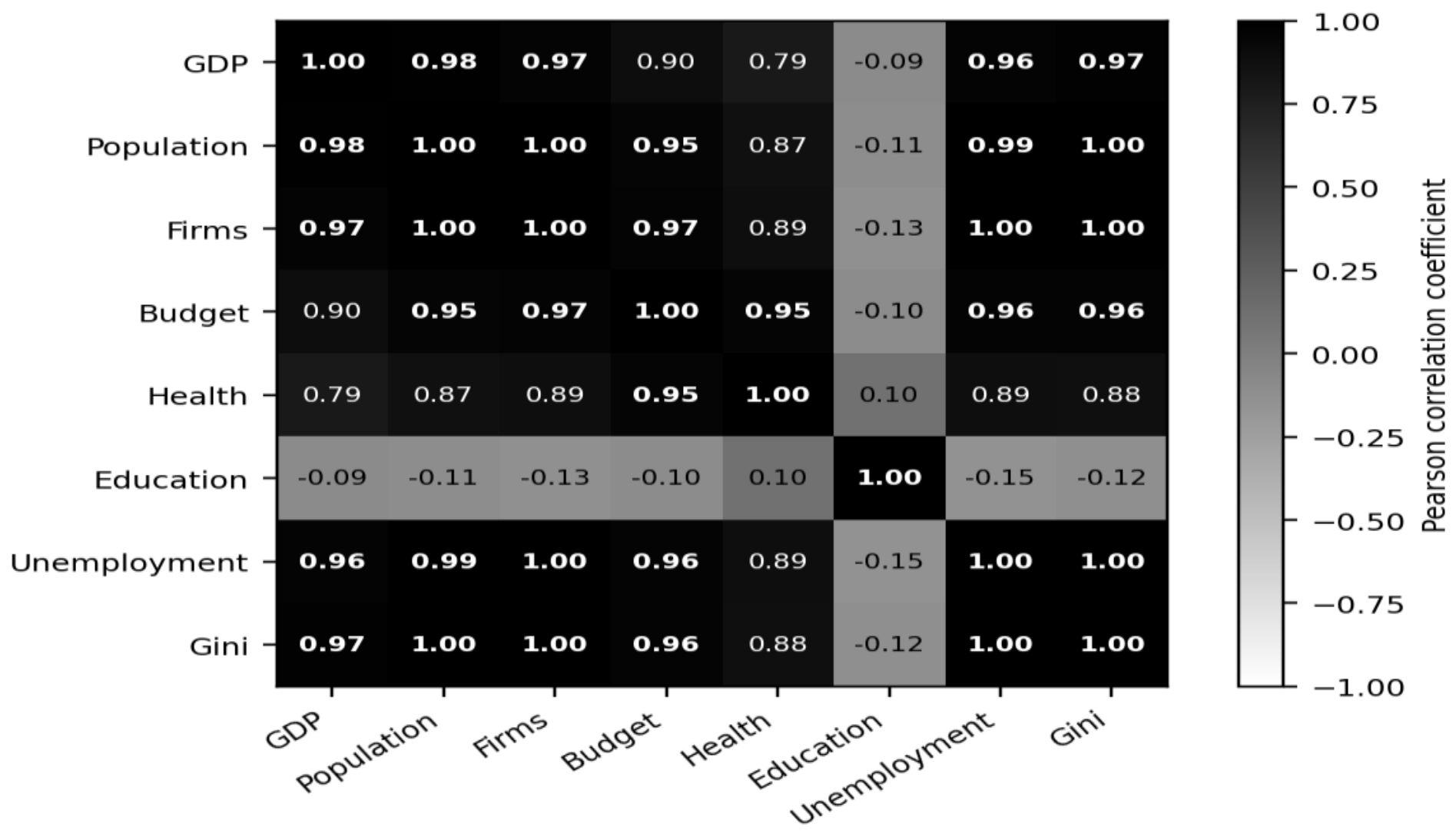
Figure 2.
Scree plot of the principal component analysis. Note: Authors’ elaboration based on the eigenvalues obtained from the principal component analysis.
Figure 2.
Scree plot of the principal component analysis. Note: Authors’ elaboration based on the eigenvalues obtained from the principal component analysis.
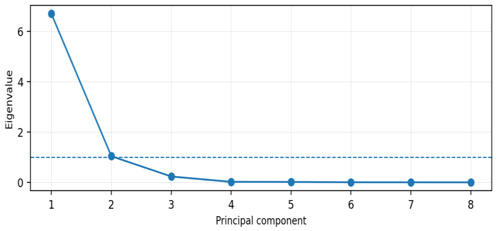
Figure 3.
Percentage decomposition of the composite index by variable and logistics complex. Note: Authors’ elaboration based on the percentage decomposition of the composite index.
Figure 3.
Percentage decomposition of the composite index by variable and logistics complex. Note: Authors’ elaboration based on the percentage decomposition of the composite index.
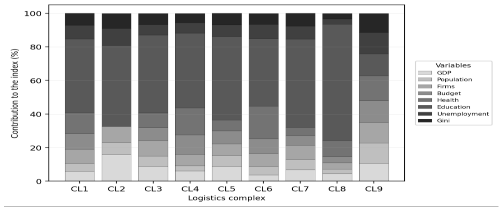
Figure 4.
Sensitivity of the composite index to the treatment of extreme values. Note: Authors’ elaboration based on the comparison between the original and Winsorized index values.
Figure 4.
Sensitivity of the composite index to the treatment of extreme values. Note: Authors’ elaboration based on the comparison between the original and Winsorized index values.
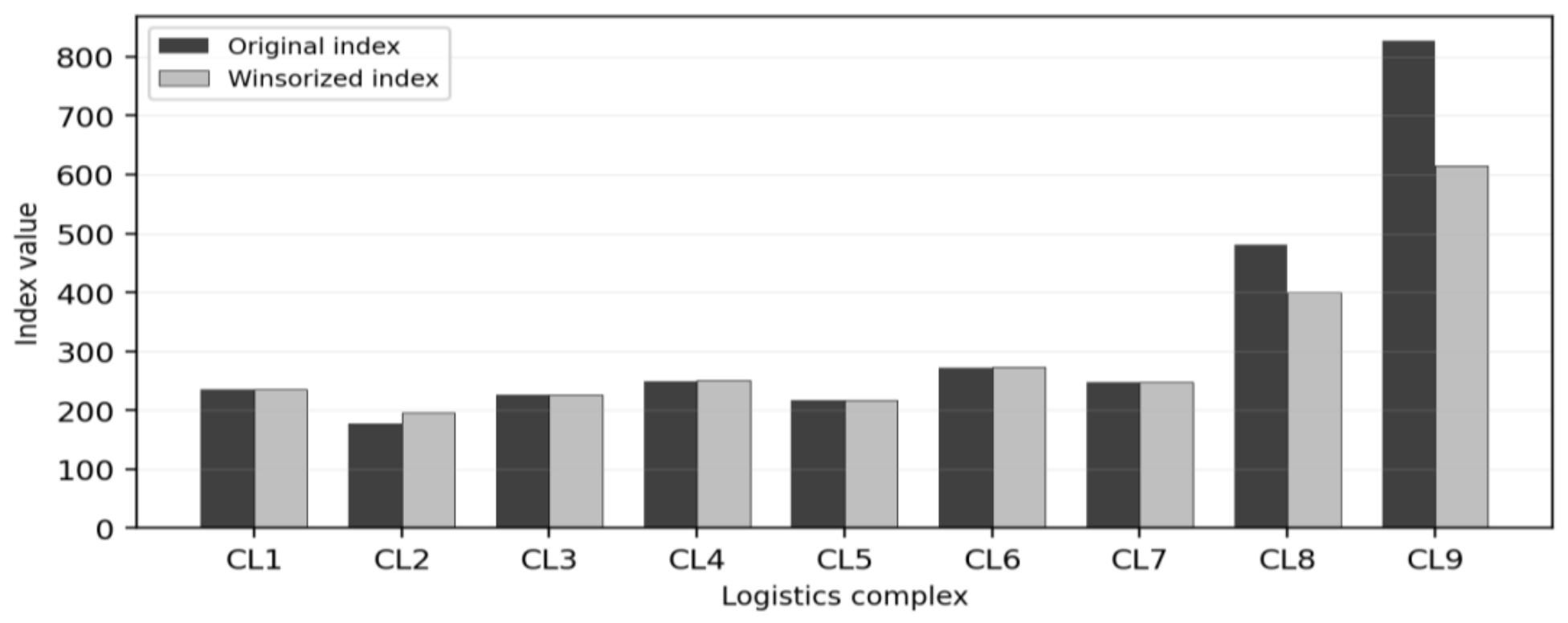
Figure 5.
Ranking of the composite socioeconomic impact index by logistics complex. Note: Authors’ elaboration based on the final ranking of the composite socioeconomic performance index.
Figure 5.
Ranking of the composite socioeconomic impact index by logistics complex. Note: Authors’ elaboration based on the final ranking of the composite socioeconomic performance index.
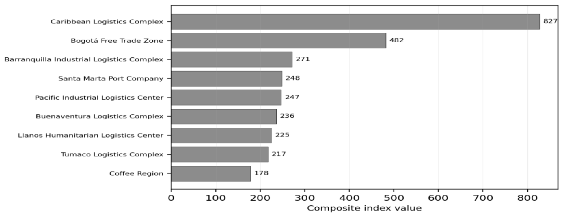
Table 1.
Variables, sources of information, and methodological treatment.
| Variable | Unit of measurement | Relationship with territorial development | Source of information | Methodological treatment |
|---|---|---|---|---|
| Gross domestic product | Millions of pesos | Positive | DANE / territorial or departmental accounts | Base-100 transformation |
| Population | Number of inhabitants | Positive | DANE / population projections | Base-100 transformation |
| Firms associated with logistics | Number of firms | Positive | Chambers of commerce / territorial business registries | Base-100 transformation |
| Municipal budget | Millions of pesos | Positive | Municipal governments / approved budgets | Harmonization into millions of pesos and base-100 transformation |
| Health investment | Millions of pesos | Positive | Territorial entities / public budgets / sectoral reports | Harmonization into millions of pesos and base-100 transformation |
| Education investment | Millions of pesos | Positive | Territorial entities / public budgets / sectoral reports | Harmonization into millions of pesos and base-100 transformation |
| Unemployment rate | Percentage | Inverse | DANE / labor market statistics | Inverse base-100 transformation |
| Gini index | Index or percentage | Inverse | DANE / territorial social statistics / official sources | Inverse base-100 transformation |
Note: Authors’ elaboration based on the variable-selection criteria, information sources, and methodological treatment defined for the study.
Table 2.
Reconstructed matrix of transformed variables of the composite index.
| Complex | GDP | Population | Firms | Budget | Health | Education | Unemployment | Gini |
|---|---|---|---|---|---|---|---|---|
| CL1 | 107,7 | 110 | 250 | 157,1 | 193,3 | 693,3 | 105,6 | 188,9 |
| CL2 | 215,4 | 130 | 212,5 | 0 | 0 | 573,3 | 100 | 177,8 |
| CL3 | 153,8 | 140 | 262,5 | 121,4 | 133,3 | 700 | 77,8 | 166,7 |
| CL4 | 115,4 | 80 | 212,5 | 207,1 | 266,7 | 740 | 83,3 | 155,6 |
| CL5 | 146,2 | 140 | 187,5 | 121,4 | 93,3 | 720 | 83,3 | 166,7 |
| CL6 | 76,9 | 140 | 262,5 | 171,4 | 353,3 | 726,7 | 127,8 | 200 |
| CL7 | 130,8 | 150 | 262,5 | 100 | 80 | 866,7 | 105,6 | 211,1 |
| CL8 | 161,5 | 140 | 225 | 128,6 | 306,7 | 2220 | 83,3 | 177,8 |
| CL9 | 669,2 | 1020 | 1262,5 | 764,3 | 820 | 720 | 583,3 | 1044,4 |
Note: Authors’ elaboration based on the reconstructed matrix of transformed variables used for the composite index.
Table 3.
Correlation matrix of the transformed variables.
| Variable | GDP | Population | Firms | Budget | Health | Education | Unemployment | Gini |
|---|---|---|---|---|---|---|---|---|
| GDP | 1 | 0,978 | 0,966 | 0,896 | 0,79 | -0,089 | 0,962 | 0,971 |
| Population | 0,978 | 1 | 0,996 | 0,954 | 0,87 | -0,106 | 0,994 | 0,998 |
| Firms | 0,966 | 0,996 | 1 | 0,966 | 0,887 | -0,127 | 0,996 | 0,998 |
| Budget | 0,896 | 0,954 | 0,966 | 1 | 0,955 | -0,095 | 0,961 | 0,962 |
| Health | 0,79 | 0,87 | 0,887 | 0,955 | 1 | 0,104 | 0,887 | 0,88 |
| Education | -0,089 | -0,106 | -0,127 | -0,095 | 0,104 | 1 | -0,148 | -0,121 |
| Unemployment | 0,962 | 0,994 | 0,996 | 0,961 | 0,887 | -0,148 | 1 | 0,998 |
| Gini | 0,971 | 0,998 | 0,998 | 0,962 | 0,88 | -0,121 | 0,998 | 1 |
Note: Authors’ elaboration based on the correlation matrix of transformed variables.
Table 5.
Eigenvalues and variance explained by component.
| Component | Eigenvalue | Explained variance (%) | Cumulative variance (%) | Decision |
|---|---|---|---|---|
| Comp. 1 | 6,688 | 83,59 | 83,59 | Retained |
| Comp. 2 | 1,039 | 12,99 | 96,58 | Retained |
| Comp. 3 | 0,233 | 2,91 | 99,49 | Complementary |
| Comp. 4 | 0,02 | 0,25 | 99,74 | Not retained |
| Comp. 5 | 0,016 | 0,2 | 99,93 | Not retained |
| Comp. 6 | 0,003 | 0,04 | 99,97 | Not retained |
| Comp. 7 | 0,002 | 0,03 | 100 | Not retained |
| Comp. 8 | 0 | 0 | 100 | Not retained |
Note: Authors’ elaboration based on the eigenvalues and explained variance obtained from the principal component analysis.
Table 6.
Factor loadings and communalities.
| Variable | Comp. 1 | Comp. 2 | Comp. 3 | Communality with 2 comp. | Communality with 3 comp. |
|---|---|---|---|---|---|
| GDP | 0,961 | 0,013 | 0,259 | 0,924 | 0,991 |
| Population | 0,994 | 0,013 | 0,097 | 0,988 | 0,997 |
| Firms | 0,997 | 0,029 | 0,042 | 0,995 | 0,997 |
| Budget | 0,978 | 0,02 | 0,175 | 0,956 | 0,987 |
| Health | 0,911 | 0,231 | 0,333 | 0,884 | 0,995 |
| Education | 0,103 | 0,99 | 0,09 | 0,992 | 1 |
| Unemployment | 0,996 | 0,049 | 0,032 | 0,994 | 0,995 |
| Gini | 0,997 | 0,025 | 0,065 | 0,994 | 0,998 |
Note: Authors’ elaboration based on factor loadings and communalities estimated for the transformed variables.
Table 7.
Comparison of weighting schemes.
| Variable | Equal weights | PCA weights | Entropy weights |
|---|---|---|---|
| GDP | 12,50% | 13,00% | 10,20% |
| Population | 12,50% | 10,00% | 18,10% |
| Firms | 12,50% | 8,00% | 11,00% |
| Budget | 12,50% | 14,00% | 16,40% |
| Health | 12,50% | 15,00% | 14,90% |
| Education | 12,50% | 15,00% | 4,30% |
| Unemployment | 12,50% | 18,00% | 13,20% |
| Gini | 12,50% | 9,00% | 12,10% |
| Total | 100% | 100% | 100% |
Note: Authors’ elaboration based on equal weights, PCA-derived weights, and entropy weights.
Table 8.
Index and ranking under three weighting schemes.
| Code | Equal-weight index | Equal-weight ranking | PCA index | PCA ranking | Entropy index | Entropy ranking |
|---|---|---|---|---|---|---|
| CL1 | 225,7 | 5 | 236 | 6 | 218,6 | 5 |
| CL2 | 176,1 | 9 | 178 | 9 | 150,3 | 9 |
| CL3 | 219,4 | 7 | 226 | 7 | 204,3 | 7 |
| CL4 | 232,6 | 4 | 249 | 4 | 233 | 4 |
| CL5 | 207,3 | 8 | 217 | 8 | 186,7 | 8 |
| CL6 | 257,3 | 3 | 272 | 3 | 269,5 | 3 |
| CL7 | 238,3 | 6 | 247 | 5 | 213,2 | 6 |
| CL8 | 430,4 | 2 | 481 | 2 | 277,6 | 2 |
| CL9 | 860,5 | 1 | 827 | 1 | 869,6 | 1 |
Note: Authors’ elaboration based on the comparison of index values and rankings under alternative weighting schemes.
Table 9.
Spearman correlation between alternative rankings.
| Ranking comparison | de Spearman | p-value | Interpretation |
|---|---|---|---|
| PCA vs. equal weights | 0,983 | < 0,001 | Very high stability |
| PCA vs. entropy | 0,983 | < 0,001 | Very high stability |
| Equal weights vs. entropy | 0,95 | < 0,001 | High stability |
Note: Authors’ elaboration based on Spearman rank correlation between alternative rankings.
Table 10.
Percentage contribution of each variable to the index by logistics complex.
| Code | GDP | Population | Firms | Budget | Health | Education | Unemployment | Gini |
|---|---|---|---|---|---|---|---|---|
| CL1 | 5,90% | 4,70% | 8,50% | 9,30% | 12,30% | 44,10% | 8,10% | 7,20% |
| CL2 | 15,70% | 7,30% | 9,60% | 0,00% | 0,00% | 48,30% | 10,10% | 9,00% |
| CL3 | 8,80% | 6,20% | 9,30% | 7,50% | 8,80% | 46,50% | 6,20% | 6,60% |
| CL4 | 6,00% | 3,20% | 6,80% | 11,60% | 16,10% | 44,60% | 6,00% | 5,60% |
| CL5 | 8,80% | 6,50% | 6,90% | 7,80% | 6,50% | 49,80% | 6,90% | 6,90% |
| CL6 | 3,70% | 5,10% | 7,70% | 8,80% | 19,50% | 40,10% | 8,50% | 6,60% |
| CL7 | 6,90% | 6,10% | 8,50% | 5,70% | 4,90% | 52,60% | 7,70% | 7,70% |
| CL8 | 4,40% | 2,90% | 3,70% | 3,70% | 9,60% | 69,20% | 3,10% | 3,30% |
| CL9 | 10,50% | 12,30% | 12,20% | 12,90% | 14,90% | 13,10% | 12,70% | 11,40% |
Note: Authors’ elaboration based on the percentage decomposition of the composite index.
Table 11.
Sensitivity of the index to P5-P95 Winsorization.
| Code | Original index | Winsorized index | Difference | Original ranking | Winsorized ranking | Change in ranking |
|---|---|---|---|---|---|---|
| CL1 | 236 | 236 | 0 | 6 | 6 | 0 |
| CL2 | 178 | 195,6 | -17,6 | 9 | 9 | 0 |
| CL3 | 226 | 226,4 | -0,4 | 7 | 7 | 0 |
| CL4 | 249 | 250,6 | -1,6 | 4 | 4 | 0 |
| CL5 | 217 | 217,8 | -0,8 | 8 | 8 | 0 |
| CL6 | 272 | 273,6 | -1,6 | 3 | 3 | 0 |
| CL7 | 247 | 247 | 0 | 5 | 5 | 0 |
| CL8 | 481 | 399,8 | 81,2 | 2 | 2 | 0 |
| CL9 | 827 | 614,6 | 212,4 | 1 | 1 | 0 |
Note: Authors’ elaboration based on the P5-P95 Winsorization sensitivity test.
Table 12.
Logistics complexes included in the analysis.
| Code | Logistics complex |
|---|---|
| CL1 | Buenaventura Logistics Complex |
| CL2 | Coffee Region |
| CL3 | Llanos Humanitarian Logistics Center |
| CL4 | Pacific Industrial Logistics Center |
| CL5 | Tumaco Logistics Complex |
| CL6 | Barranquilla Industrial Logistics Complex |
| CL7 | Santa Marta Port Company |
| CL8 | Bogotá Free Trade Zone |
| CL9 | Caribbean Logistics Complex |
Note: Authors’ elaboration based on the logistics complexes included in the empirical analysis.
Table 13.
Estimated weights for the composite index variables.
| Variable | Representation | Component | Scoring coefficient | |
|---|---|---|---|---|
| GDP | X1 | Comp. 1 | 0,4196 | 13% |
| Population | X2 | Comp. 1 | 0,3235 | 10% |
| Number of firms associated with business logistics | X3 | Comp. 2 | 0,2492 | 8% |
| Municipal budget | X4 | Comp. 1 | 0,4488 | 14% |
| Health investment | X5 | Comp. 1 | 0,4741 | 15% |
| Education investment | X6 | Comp. 2 | 0,4763 | 15% |
| Unemployment rate | Y1 | Comp. 3 | 0,5738 | 18% |
| Gini index | Y2 | Comp. 3 | 0,2948 | 9% |
| Total | 3,26 | 100% | ||
Note: Authors’ elaboration based on the estimated weights obtained for the composite index variables.
Table 14.
Baseline values of the variables by logistics complex.
| Variable | Rep. | CL1 | CL2 | CL3 | CL4 | CL5 | CL6 | CL7 | CL8 | CL9 |
|---|---|---|---|---|---|---|---|---|---|---|
| GDP | X1 | 54.353 | 106.819 | 35.331 | 44.570 | 10.991 | 38.575 | 10.514 | 50.202 | 67.245 |
| Population | X2 | 362.764 | 467.185 | 531.275 | 1.822.871 | 990.179 | 1.228.271 | 311.761 | 5.828.528 | 887.946 |
| Number of firms associated with business logistics | X3 | 66 | 50 | 55 | 68 | 44 | 60 | 60 | 46 | 68 |
| Municipal budget (in millions) | X4 | 298.937 | 2.460.000 | 729.945 | 2.027.683 | 770.439 | 2.347.475 | 822.174 | 3.825.826 | 1.071.227 |
| Health investment | X5 | 64.839 | 965.000 | 69.977 | 401.524 | 112.787 | 184.198 | 64.736 | 345.827 | 163.116 |
| Education investment | X6 | 114.993 | 228.874 | 284.345 | 563.575 | 395.895 | 369.483 | 111.618 | 57.680 | 275.981 |
| Unemployment rate | Y1 | 40% | 43,80% | 11,90% | 11,50% | 13,70% | 7,20% | 15,70% | 11,40% | 6,70% |
| Gini index | Y2 | 43,50% | 29,30% | 24,30% | 21,60% | 34,80% | 25,60% | 34% | 40% | 29,20% |
Note: Authors’ elaboration based on the baseline values compiled for each logistics complex.
Table 15.
Follow-up values reconstructed from the baseline and from the transformations of the composite index.
Table 15.
Follow-up values reconstructed from the baseline and from the transformations of the composite index.
| Variable | Rep. | CL1 | CL2 | CL3 | CL4 | CL5 | CL6 | CL7 | CL8 | CL9 |
|---|---|---|---|---|---|---|---|---|---|---|
| GDP | X1 | 58.538 | 230.088 | 54.339 | 51.434 | 16.069 | 29.664 | 13.752 | 81.076 | 450.004 |
| Population | X2 | 399.040 | 607.341 | 743.785 | 1.458.297 | 1.386.251 | 1.719.579 | 467.642 | 8.159.939 | 9.057.049 |
| Number of firms associated with business logistics | X3 | 165 | 106 | 144 | 83 | 83 | 158 | 158 | 104 | 859 |
| Municipal budget (in millions) | X4 | 469.630 | 0 | 886.153 | 4.199.331 | 935.313 | 4.023.572 | 822.174 | 4.920.012 | 8.187.388 |
| Health investment | X5 | 125.334 | 0 | 93.279 | 1.070.865 | 105.230 | 650.772 | 51.789 | 1.060.651 | 1.337.551 |
| Education investment | X6 | 797.246 | 1.312.135 | 1.990.415 | 4.170.455 | 2.850.444 | 2.685.033 | 967.393 | 1.280.496 | 1.987.063 |
| Unemployment rate | Y1 | 37,88% | 43,80% | 15,30% | 13,81% | 16,45% | 5,63% | 14,87% | 13,69% | 1,15% |
| Gini index | Y2 | 23,03% | 16,48% | 14,58% | 13,88% | 20,88% | 12,80% | 16,11% | 22,50% | 2,80% |
Note: Authors’ elaboration based on the reconstructed follow-up values and transformations of the composite index.
Table 16.
Composite socioeconomic impact index by logistics complex.
| Variable | Representation | CL1 | CL2 | CL3 | CL4 | CL5 | CL6 | CL7 | CL8 | CL9 |
|---|---|---|---|---|---|---|---|---|---|---|
| GDP | X1 | 14 | 28 | 20 | 15 | 19 | 10 | 17 | 21 | 87 |
| Population | X2 | 11 | 13 | 14 | 8 | 14 | 14 | 15 | 14 | 102 |
| Number of firms associated with business logistics | X3 | 20 | 17 | 21 | 17 | 15 | 21 | 21 | 18 | 101 |
| Municipal budget | X4 | 22 | 0 | 17 | 29 | 17 | 24 | 14 | 18 | 107 |
| Health investment | X5 | 29 | 0 | 20 | 40 | 14 | 53 | 12 | 46 | 123 |
| Education investment | X6 | 104 | 86 | 105 | 111 | 108 | 109 | 130 | 333 | 108 |
| Unemployment rate | Y1 | 19 | 18 | 14 | 15 | 15 | 23 | 19 | 15 | 105 |
| Gini index | Y2 | 17 | 16 | 15 | 14 | 15 | 18 | 19 | 16 | 94 |
| Index | 236 | 178 | 225 | 247 | 217 | 271 | 248 | 482 | 827 | |
Note: Authors’ elaboration based on the weighted transformed variables and final composite index.
Table 17.
Qualitative classification of socioeconomic impact by logistics complex.
| Code | Logistics complex | Composite index | Impact category |
|---|---|---|---|
| CL1 | Buenaventura Logistics Complex | 236 | Very high impact |
| CL2 | Coffee Region | 178 | Very high impact |
| CL3 | Llanos Humanitarian Logistics Center | 225 | Very high impact |
| CL4 | Pacific Industrial Logistics Center | 247 | Very high impact |
| CL5 | Tumaco Logistics Complex | 217 | Very high impact |
| CL6 | Barranquilla Industrial Logistics Complex | 271 | Very high impact |
| CL7 | Santa Marta Port Company | 248 | Very high impact |
| CL8 | Bogotá Free Trade Zone | 482 | Very high impact |
| CL9 | Caribbean Logistics Complex | 827 | Very high impact |
Note: Authors’ elaboration based on the qualitative scale defined for the composite index.
Table 18.
Complementary classification of the relative performance of the composite index.
| Composite index range | Relative performance category | Interpretive criterion |
|---|---|---|
| 175–250 | Moderate very high impact | The complex substantially exceeds the baseline, but its relative performance remains within the lower group of the very high category. |
| 251–350 | Consolidated very high impact | The complex shows performance above the moderate group, with more consistent improvements across several dimensions of the index. |
| 351–600 | Outstanding impact | The complex presents a level of impact considerably above the average of the analyzed set. |
| More than 600 | Exceptional impact | The complex records an extreme performance within the sample, associated with very high improvements in several transformed variables. |
Note: Authors’ elaboration based on the complementary classification developed for the upper range of the index.
Table 19.
Relative performance classification by logistics complex.
| Code | Logistics complex | Composite index | Initial qualitative classification | Complementary classification |
|---|---|---|---|---|
| CL1 | Buenaventura Logistics Complex | 236 | Very high impact | Moderate very high impact |
| CL2 | Coffee Region | 178 | Very high impact | Moderate very high impact |
| CL3 | Llanos Humanitarian Logistics Center | 225 | Very high impact | Moderate very high impact |
| CL4 | Pacific Industrial Logistics Center | 247 | Very high impact | Moderate very high impact |
| CL5 | Tumaco Logistics Complex | 217 | Very high impact | Moderate very high impact |
| CL6 | Barranquilla Industrial Logistics Complex | 271 | Very high impact | Consolidated very high impact |
| CL7 | Santa Marta Port Company | 248 | Very high impact | Moderate very high impact |
| CL8 | Bogotá Free Trade Zone | 482 | Very high impact | Outstanding impact |
| CL9 | Caribbean Logistics Complex | 827 | Very high impact | Exceptional impact |
Note: Authors’ elaboration based on the relative performance classification of the logistics complexes.
Disclaimer/Publisher’s Note: The statements, opinions and data contained in all publications are solely those of the individual author(s) and contributor(s) and not of MDPI and/or the editor(s). MDPI and/or the editor(s) disclaim responsibility for any injury to people or property resulting from any ideas, methods, instructions or products referred to in the content. |
© 2026 by the authors. Licensee MDPI, Basel, Switzerland. This article is an open access article distributed under the terms and conditions of the Creative Commons Attribution (CC BY) license (http://creativecommons.org/licenses/by/4.0/).
Copyright: This open access article is published under a Creative Commons CC BY 4.0 license, which permit the free download, distribution, and reuse, provided that the author and preprint are cited in any reuse.


