
Submitted:
03 August 2026
Posted:
04 August 2026
You are already at the latest version
Abstract
In application scenarios such as medical imaging and industrial inspection, object detection models are often trained on grayscale images but deployed under mixed grayscale–RGB inputs. Experimental observations reveal a pronounced asymmetry in this setting: models trained on RGB datasets generalize well to grayscale detection tasks, whereas models trained on grayscale datasets exhibit severe performance degradation and substantial inter-run variability when applied to RGB inputs. This phenomenon significantly limits practical deployment and cannot be fully explained by the conventional assumption that grayscale training lacks chromatic information.In this work, we analyze the chromatic information processing mechanism in the first layer (layer 0) of YOLO-based object detection models. We reveal that training on grayscale samples induces variance collapse in chromatic channels, and further elucidate how this mechanism leads to RGB detection mismatch. Based on this analysis, we propose a kernel-aware regularization method that adjusts the chromatic sensitivity of the first layer by modulating the ratio between chromatic and luminance channels, thereby effectively mitigating the impact of variance collapse.Experimental results demonstrate that the proposed method reduces the mAP50 drop of YOLO grayscale models on RGB detection from 10% ~ 20% to 1% ~ 2%. It also effectively alleviates performance degradation in RTDETR and FasterRCNN under the same cross-modal scenarios, significantly improving the robustness of model training with respect to variations in input data distribution.
Keywords:
convolutional neural networks
; chromatic mismatch
; ColorScore
; feature channel allocation
; chromatic-sensitivity regularization
; chromatic variance collapse
1. Introduction
Convolutional neural network (CNN)-based object detection models have been widely applied across numerous domains. Representative detectors such as YOLO, DETR, and Faster R-CNN are typically fine-tuned from pretrained weights learned on large-scale RGB datasets. However, when the fine-tuning data consists of grayscale images, these models often encounter a modality mismatch between grayscale training and RGB deployment [1]. For instance, in medical imaging, X-ray and CT scans are inherently grayscale but are frequently stored in RGB formats in DICOM files; in industrial inspection, upgrades from grayscale cameras to color cameras require legacy models trained on grayscale data to process RGB inputs. In these scenarios, computational resources and real-time constraints on edge devices often necessitate the deployment of lightweight end-to-end detectors such as YOLO, making it difficult to directly adopt large vision models for cross-modal adaptation [2].
A shared characteristic of these settings is that models are trained on grayscale data but are required to maintain detection performance under RGB inputs. Experimental results reveal a pronounced asymmetry in this modality adaptation process: models trained on RGB data generally retain satisfactory performance when applied to grayscale inputs, whereas models trained on grayscale data suffer from severe performance degradation when applied to RGB inputs, along with substantial variability across different training runs. This modality shift between grayscale and RGB primarily manifests as a mismatch in chromatic channel information, referred to as the color mismatch problem. Importantly, this asymmetry cannot be fully explained by the conventional assumption that grayscale training lacks chromatic information, indicating the presence of deeper underlying mechanisms.
Figure 1 illustrates comparative results using three detectors: YOLO26s [3] , RTDETR-L [4] , and Faster R-CNN [5]. Subfigure (A) shows the validation results of model fine-tuned from pretrained parameters on a grayscale dataset (hereafter “grayscale models”), while subfigure (B) shows the results of model fine-tuned from pretrained parameters on an RGB dataset (hereafter “RGB models”). In both subfigures, red curves indicate performance on RGB validation images, and blue curves indicate performance on grayscale validation images. Each model was trained and validated 10 times; the x-axis represents the N-th training-validation run, and the y-axis shows the mAP@0.5 (mAP50) metric. As shown, the RGB models in (B) generalize reasonably well to grayscale images, whereas the grayscale models in (A) consistently exhibit substantial performance degradation under cross-modality evaluation. Notably, YOLO26s and RTDETR-L display pronounced fluctuations in performance across different training runs.
For the aforementioned color mismatch problem, existing studies commonly attribute its cause to a discrepancy between training and deployment conditions. Specifically, open-source models are typically trained on datasets containing only a limited proportion of grayscale images, resulting in weak task specificity for grayscale scenarios. Conversely, models trained on grayscale images are unable to learn chromatic features present in RGB images, leading to more severe degradation in cross-domain performance.
To address the limitations of existing models in handling chromatic mismatch, prior studies have explored approaches based on color invariance or color augmentation [6,7], aiming to develop deep representations that are independent of color, thereby enhancing robustness to color variations. Lengyel et al.[8] introduced color-equivariant convolutional operations, sharing parameters across hue transformations to preserve discriminative information while improving color robustness. Yang et al.[9] further leveraged a group convolution framework to construct network architectures that are equivariant to changes in hue, saturation, and brightness.
These studies effectively improve model robustness under color mismatch scenarios, but the proposed enhancements primarily target color models and do not account for the pronounced fluctuations observed in the grayscale models of Figure 1(A). To elucidate the mechanisms underlying these phenomena, this study analyzes the channel-wise processing of chromatic information in the first layer of relevant models, revealing the process by which variance collapse occurs during grayscale training and clarifying its relationship to performance degradation under color mismatch. Based on this analysis, we define a parameter for quantifying the chromatic sensitivity of convolutional kernels—ColorScore and propose a kernel-level chromatic sensitivity regularization method. This approach allows control over the channel bias between chromatic and luminance components during training, effectively mitigating cross-color-domain instability and enhancing model performance under color mismatch conditions. The primary contributions of this work are as follows:
1.Analysis of RGB detection mismatch mechanism. By examining the chromatic information processing in the first layer (layer 0) of YOLO models, we reveal the core mechanism by which training on grayscale samples induces variance collapse, ultimately leading to RGB detection mismatch.
2.Chromatic-Sensitivity Regularization. Building on the RGB detection mismatch analysis, we propose a kernel-level regularization method that adjusts the chromatic sensitivity of the first layer by modulating the ratio between color-channel kernels and luminance-channel kernels. This effectively mitigates the impact of variance collapse. Experiments demonstrate that this approach is also effective for CNN models with first-layer structures similar to YOLO, indicating its potential to enhance robustness of model training across diverse input samples.
3.ColorScore metric for chromatic sensitivity. We introduce a ColorScore parameter to quantify the chromatic sensitivity of convolutional kernels. This metric allows analysis of whether a kernel preferentially extracts chromatic or luminance information.
2. Related Work
2.1. Mechanisms of Color Information in CNN Models
Existing studies generally agree that CNNs can leverage color information to enhance visual task performance, but the extent of this reliance is highly task-dependent and data-dependent. Singh et al.[10] demonstrated that CNNs often depend on color cues, which may vary significantly across different scenarios. Bhatta et al.[11] found that, in face recognition tasks, models trained on grayscale images can achieve performance comparable to color-trained models, suggesting that structural and textural information may be more critical than color in certain tasks.
Some researchers have attempted to reduce model sensitivity to color anomalies through modeling strategies. For example, Chen and Yang et al.[12] designed no-reference color loss functions to prevent the impact of outlier values in individual RGB channels during nighttime image fusion. Building on this, Xie and Fan et al.[13] introduced color space transformation operations to further enhance robustness to color variations.
From the perspective of internal network mechanisms, prior work has begun to analyze how CNNs encode color information within feature representations [14,15,16]. For instance, Flachot and Gegenfurtner [17] examined the color sensitivity of individual CNN units, revealing that color-selective neurons are present across layers, with deeper layers exhibiting stronger specialization. Similarly, Rafegas and Vanrell [18] constructed color-selectivity metrics to characterize the chromatic properties of neurons. Cesteros and Rincon [19] showed that introducing long skip connections increases the number of highly color-sensitive neurons. Harris et al.[20] demonstrated that CNNs can develop color-opponent representations similar to those observed in biological visual systems [21,22].
2.2. Impact of Color Space Selection on CNN Performance
In terms of color representation, the choice of color space has been shown to significantly affect model performance. Fundamentally, different color spaces modify the coupling between luminance and chrominance, thereby influencing how CNNs encode visual information. Yeu et al.[23] conducted the first systematic study on the effect of color spaces on object detection models under low-light conditions, demonstrating that selecting an appropriate color space can substantially improve detection performance in nighttime scenes. Dobrzycki and Bernardos [24], using the YOLOv8s model, performed comparative experiments across multiple color spaces in military scenarios, validating that different color representations affect detection stability. Additionally, Xian et al.[25] and Mitlo et al.[26] explored the combination of various color spaces (e.g., RGB, HSV, Lab) with different CNN architectures, investigating how color space selection impacts classification and detection performance.
Existing studies suggest that different color spaces can enhance performance under specific conditions, such as low illumination or specialized tasks. However, RGB remains the mainstream choice, providing stable performance across most general visual tasks. Notably, prior work has primarily focused on input space selection and transformation, with limited analysis from the perspective of internal network representation mechanisms, leaving open questions on how color information influences network stability and cross-modal generalization.
2.3. Cross-Modal Domain Adaptation and Feature Alignment
From a more general perspective, the discrepancy between grayscale and RGB images can be regarded as a special case of cross-modal domain adaptation, where the source and target domains differ in both statistical distribution and information representation. In recent years, cross-modal domain adaptation methods have provided valuable insights into this problem from multiple angles.For example, D et al.[27] addressed the visible-to-infrared adaptation problem by proposing a semantic-aware grayscale augmentation (SAGA) strategy, which converts RGB images into grayscale at the instance level to reduce color bias and narrow the modality gap between visible and infrared domains. Wang et al.[28] proposed CM-YOLO, which learns infrared–visible feature mappings via a modality translation module to achieve cross-modal alignment in the feature space. Zhao et al.[29] introduced a correlation-driven decomposition loss to explicitly disentangle modality-shared and modality-specific features, providing a structured framework for cross-modal knowledge transfer. In addition, teacher–student-based cross-modal knowledge distillation methods have also been widely explored [30,31].
These studies suggest that cross-modal performance discrepancies are not only caused by differences in information content, but are also closely related to mismatches in feature distributions and statistical properties. Accordingly, explicit modeling of modality gaps—such as feature alignment, feature disentanglement, and modality translation—has proven to be an effective strategy for mitigating such issues. However, most existing cross-modal domain adaptation methods rely on target-domain data (at least unlabeled samples) for post hoc alignment, or introduce additional architectures (e.g., modality translators or multi-branch networks) to bridge an already-formed modality gap. They rarely intervene at the root cause of modality divergence during the training process itself.
3. Analysis of the Color Mismatch Problem
Figure 2 illustrates the color mismatch scenarios for four models: YOLOv5su [32], YOLOv8s [33], YOLO11s, and YOLO26s. All models are first fine-tuned on grayscale and RGB training datasets, respectively, and then evaluated on both grayscale and RGB test datasets. Each fine-tuning process is conducted for 100 epochs using the AdamW optimizer, with an initial learning rate of and a batch size of 32. The dataset used is PASCAL VOC2007, along with its corresponding converted grayscale version.
The reason for selecting this dataset is that the focus of this study is to reveal the intrinsic mechanism underlying RGB detection degradation caused by grayscale training, namely variance collapse, rather than to optimize performance for a specific application scenario. As a standard benchmark for RGB object detection, PASCAL VOC2007 can be converted into a grayscale version while preserving identical semantic content, thereby isolating color information as the only varying factor. This enables a clearer observation of the variance collapse phenomenon and its impact on detection performance.The variance collapse mechanism revealed in this work originates from the weight degradation process of convolutional kernels in the first layer (layer 0) under grayscale training. Since this process is independent of specific image content, the findings obtained on a general-purpose dataset provide a solid theoretical basis for transferability to real-world scenarios such as medical imaging and industrial inspection.
As shown in Figure 2, compared with the performance degradation observed when RGB models are validated on grayscale images in region (B), the degradation is substantially more severe when grayscale models are validated on RGB images in region (A), accompanied by significant fluctuations across different training runs. This clearly indicates deficiencies in the models’ handling of chromatic information. From an architectural perspective, the first stage of such processing corresponds to the initial layer (layer 0) of the model, as illustrated in Figure 3.
Let the convolutional kernels of layer 0 be denoted as , where correspond to the convolutional kernel parameters for the three input channels, and is the kernel size. Consider an input sample , where represent the data in the red, green, and blue channels, respectively. The luminance L is defined as:
Then we have:
where can be regarded as the color components corresponding to each channel. The convolution result can thus be expressed as:
Let . The values of the convolutional kernels in the first layer (layer 0) of the YOLO26s model were computed, and their absolute values are listed in Figure 4. It can be observed that some channels exhibit very small weight magnitudes, with channels 5, 6, 12, 14, 17, 23, and 30 having weights below 0.05. Similar computations of for the first layer of the other three models reveal the presence of comparable channels.
According to Equation (3), these channels show relative insensitivity to the L component of the input RGB image. In this study, such convolutional kernels are referred to as chromatic filters, and the channels in which they reside are referred to as chromatic channels. These channels primarily process the chromatic information present in the input image.
When the training data consists of grayscale images, the inputs in Equation (3) satisfy , and the expression degenerates accordingly:
At this stage, due to the influence of the kernel weight coefficients, the outputs of the chromatic filters become significantly reduced, which in turn affects the Batch Normalization (BN) layer according to the following variance update formulation:
Here, and denote the global variance parameter of the channel output and the variance of the current batch, respectively.
During grayscale model training, the convolutional outputs of chromatic channels decrease, leading to smaller values of and . After multiple updates, the global variance correspondingly diminishes substantially. Figure 5 illustrates the BN variance parameters of each channel in the first layer for both grayscale and RGB models trained using four YOLO variants. In the figure, the red curves represent the RGB models, while the blue curves represent the grayscale models; the horizontal axis denotes the channel index, and the vertical axis denotes the variance value.
It can be observed that, in grayscale models, the BN variance of certain channels decreases by orders of magnitude compared with that of RGB models. This phenomenon is referred to as chromatic variance collapse. A comparison between Figure 4 and Figure 5 shows that the channel indices exhibiting variance collapse in the YOLO26 model strongly correlate with the chromatic channel indices identified in Figure 4, which is consistent with the aforementioned theoretical analysis.
The output of the first layer (layer 0) of YOLO models is given by Equation (8).
Analysis indicates that during grayscale model training, the reduced outputs of chromatic channels not only lead to variance collapse in order to accommodate this change, but may also increase perturbations in the optimization of chromatic channel convolutional kernels. This can further cause the model to compromise its overall performance in order to achieve parameter convergence. When RGB information is reintroduced, the collapsed variances in the denominator of Equation (8) amplify these perturbations in the chromatic channels, which may ultimately result in substantial fluctuations in performance across different training runs.
In contrast, for the scenario where RGB models are validated on grayscale datasets, the chromatic channels are not affected by insufficient information during training. During validation, since the input grayscale images lack chromatic information, the chromatic channels contribute little to the detection results, leading to reduced performance; however, the absence of variance collapse prevents the occurrence of large performance fluctuations.
4. Chromatic-Sensitivity Regularization
To address the aforementioned color mismatch problem, we design a metric to quantify the chromatic sensitivity of channel-wise convolutional kernels. Based on this metric, we propose a channel-distribution–based chromatic sensitivity regularization method, which improves the robustness of detection models by controlling the performance and distribution of chromatic channels in the first layer (layer 0).
4.1. Convolutional Kernel Chromatic Sensitivity Score
We introduce the ColorScore parameter to measure the sensitivity of convolutional filters to chromatic information, facilitating the identification of chromatic kernels and their corresponding channels. Each convolutional kernel within a channel is treated as a three-dimensional vector:
The luminance basis vector is defined as follows:
The weight vector of each convolutional kernel is then decomposed into luminance and chromatic components:
We define:
From the above formulation, it can be observed that when the chromatic component dominates within a convolutional kernel, the corresponding ColorScore value becomes larger. In such cases, the filter exhibits reduced sensitivity to luminance information and increased sensitivity to chromatic information.
Figure 6 presents the ColorScore values for each channel in four YOLO model variants. A comparison with Figure 5 shows that the channels exhibiting variance collapse by orders of magnitude correspond to those with relatively high ColorScore values. In this study, channels with ColorScore values greater than 0.9 are identified as chromatic channels, which serve as the basis for subsequent analysis and regularization.
4.2. Chromatic Sensitivity Regularization Method
We control variance collapse in chromatic channels under grayscale training from two perspectives. First, we promote differentiation of chromatic sensitivity across channels: increasing the chromatic sensitivity of chromatic channels while reducing the chromatic sensitivity of other channels. Second, we appropriately control the number of chromatic channels to mitigate performance loss during grayscale training. To achieve this, we construct two loss terms, and . The loss is defined as follows:
Here denotes the ColorScore of the -th channel, is the total number of channels in the first layer (layer 0), and is a preset total chromatic sensitivity score. This loss term allows control over the number of chromatic channels in layer 0 via the parameter : larger values of lead to more chromatic channels, while smaller values reduce their number.
The loss , is defined as follows:
is minimized when or 1, and maximized at . This term encourages functional differentiation between channels, reducing ambiguous or overlapping roles.
The two loss terms are combined with the model’s original detection loss for regularization, as expressed in Equation (16), where denotes the original detection training loss of the model.
5. Experiments
All experiments are conducted on the PASCAL VOC2007 dataset and its corresponding grayscale version. For the regularized training experiments, the training settings are unified as follows: 100 epochs, the AdamW optimizer, an initial learning rate of , and a batch size of 32.
5.1. Effectiveness of Chromatic Sensitivity Regularization
Figure 7 presents the validation results of four YOLO grayscale models with regularization applied under the setting . The red curves correspond to validation on RGB data, while the blue curves correspond to validation on grayscale data. Each model is trained and evaluated 10 times, where the horizontal axis represents the -th run and the vertical axis denotes the mAP50 performance.
A comparison between Figure 2(A) and Figure 7 shows that the proposed regularization method significantly improves the detection performance of grayscale models on RGB samples. Moreover, the severe performance fluctuations observed across different training runs are effectively eliminated.
Figure 8 shows the ColorScore values of the first-layer channels for the four YOLO grayscale models with regularization applied under . TThe horizontal axis represents the channel index of layer 0, and the vertical axis denotes the ColorScore values. Compared with the left panel of Figure 6, it is evident that the number of chromatic channels has decreased significantly, and the functional differentiation among channels is more pronounced. This demonstrates the effectiveness of chromatic sensitivity regularization in regulating channel allocation during model training.
5.2. Generalization of Chromatic Sensitivity Regularization
To evaluate the generality of the proposed regularization method, we select the RTDETR-L and FasterRCNN models, which exhibit behaviors similar to those observed in Figure 1(A), for further testing. The backbone of RTDETR-L is a CNN-based HGNetv2 network, followed by a hybrid encoder based on Vision Transformers. The FasterRCNN model uses a ResNet50 backbone.
Figure 9 shows the experimental results under the setting . It can be observed that grayscale models trained with the proposed regularization exhibit significantly improved performance and stability when validated on RGB data compared with non-regularized models. This confirms the effectiveness of the method for models employing similar backbone architectures.
5.3. Analysis of the Chromatic Sensitivity Regularization Parameter
To investigate the effect of different values on regularization outcomes, experiments were conducted on the four grayscale YOLO models under varying settings. The results are summarized in Table 1, where each value represents the average of 10 validation runs. In the baseline models, the initial values for all channels across the four models were approximately 15. Consequently, setting to 3, 6, or 8 effectively reduces the number of chromatic channels, whereas increases the number of chromatic channels.
Table 1 shows that for YOLOv5su, YOLO11s, and YOLO26s, grayscale models with ,6 or 8 exhibit significantly improved RGB detection performance. The results for YOLOv8s differ slightly: although its baseline is also approximately 15, the model contains 8 chromatic channels (as shown in Figure 6). Therefore, when or 8,the actual number of chromatic channels does not decrease effectively, limiting the impact of the regularization.
When is set to 18 or 24, the RGB detection performance of all four models shows a general decline. This indicates that further increasing the number of chromatic channels does not improve the model’s utilization of color information in RGB images, and may in fact interfere with the extraction of luminance information.
For color models, experiments were conducted using two extreme strategies, and , with results summarized in Table 2. It can be observed that introducing chromatic sensitivity regularization results in only a minor decline in grayscale validation performance compared with the baseline models (approximately mAP50), indicating that the proposed regularization does not compromise the original capabilities of RGB models.
Furthermore, even under , the detection performance of color models in the RGB space remains largely unchanged. This suggests that the models retain strong capability to leverage color information even when chromatic channels are suppressed. The precise mechanisms underlying this phenomenon require further investigation.
5.4. Ablation Study

Table 3.
Ablation experiment of color sensitivity regularization loss.
| Parameter Settings | YOLO26s Model mAP50 Value | |||
| Gray | Color | |||
| 0.8450.004 | 0.5920.070 | |||
| √ | 0.8420.004 | 0.5550.028 | ||
| √ | 0.8350.008 | 0.8290.006 | ||
| √ | √ | 0.8410.004 | 0.8330.004 | |
The ablation results indicate that is the primary factor contributing to improved chromatic robustness of the model. In contrast, helps enhance the stability of model performance by reducing variability across training runs. However, when used independently, does not improve RGB detection performance; instead, it may lead to performance degradation due to overly strong channel disentanglement constraints. When the two loss terms are jointly applied, plays a complementary regularization role, further refining channel specialization and enabling the model to achieve optimal overall performance.
6. Conclusions
This paper systematically investigates the color mismatch phenomenon in YOLO models when training data is converted from RGB to grayscale. We analyze the relationship between the chromatic sensitivity of channel-wise convolutional filters and variance collapse in Batch Normalization layers, and propose a chromatic sensitivity regularization method based on the ColorScore metric to control channel allocation within the model.
Experimental results demonstrate that, with the proposed chromatic sensitivity regularization, the performance degradation of grayscale-trained models on RGB inputs is reduced from 10% ~ 20% to 1% ~ 2%, while also effectively eliminating performance fluctuations across different training runs. The proposed method is also effective for classical CNN-based detectors such as RTDETR-L and Faster R-CNN. Overall, this approach improves the robustness of model training with respect to data distribution shifts and provides a useful reference for CNN-based object detection in real-world scenarios where grayscale training and RGB deployment coexist, such as medical imaging, industrial inspection, and infrared surveillance.
Author Contributions
Z.W., T.C., and J.Y. wrote the main manuscript text.Z.W. conducted the main experiments and data collection.Z.Y. and K.Q. performed additional experiments.All authors reviewed the manuscript.
Funding
This research did not receive any specific grant from funding agencies in the public, commercial, or not-for-profit sectors.
Institutional Review Board Statement
Not applicable.
Informed Consent Statement
Not applicable.
Data Availability Statement
The datasets used in this study are publicly available. PASCAL VOC2007 dataset was used and its grayscale version was generated by converting the original RGB images. The processed data can be reproduced from the original dataset following the procedure described in the paper.
Conflicts of Interest
The authors have no relevant financial or non-financial interests to disclose.
References
- Ramakrishnan, R. Domain Adaptation in Multimodal Models. In Transfer Learning - Unlocking the Power of Pretrained Models; Mazzeo, P.L., Bruno, A., Eds.; IntechOpen: London, 2025. [Google Scholar]
- Xu, Y.; Khan, T.M.; Song, Y.; Meijering, E. Edge deep learning in computer vision and medical diagnostics: a comprehensive survey. Artif. Intell. Rev. 2025, 58, 93. [Google Scholar] [CrossRef]
- Jocher, G.; Qiu, J. Ultralytics YOLO26, 26.0.0 2026. [CrossRef]
- Zhao, Y.; Lv, W.; Xu, S.; Wei, J.; Wang, G.; Dang, Q.; Liu, Y.; Chen, J. DETRs Beat YOLOs on Real-time Object Detection. Proc. 2024 IEEE/CVF Conf. Comput. Vis. Pattern Recognit. (CVPR) 2024, 2024, 16965–16974. [Google Scholar] [CrossRef]
- Ren, S.; He, K.; Girshick, R.; Sun, J. Faster R-CNN: Towards Real-Time Object Detection with Region Proposal Networks. IEEE Trans. Pattern Anal. Mach. Intell. 2017, 39, 1137–1149. [Google Scholar] [CrossRef] [PubMed]
- Flachot, A.; Akbarinia, A.; Schütt, H.H.; Fleming, R.W.; Wichmann, F.A.; Gegenfurtner, K.R. Deep neural models for color classification and color constancy. J. Vis. 2022, 22, 17–17. [Google Scholar] [CrossRef] [PubMed]
- Heidari-Gorji, H.; Gegenfurtner, K.R. Object-based color constancy in a deep neural network. J. Opt. Soc. Am. A 2023, 40, A48–A56. [Google Scholar] [CrossRef] [PubMed]
- Lengyel, A.; Strafforello, O.; Bruintjes, R.-J.; Gielisse, A.; van Gemert, J. Color Equivariant Convolutional Networks. arXiv 2023, arXiv:2310.19368. [Google Scholar] [CrossRef]
- Yang, Y.; O’Mahony, F.; Allen-Blanchette, C. Learning Color Equivariant Representations. arXiv 2024, arXiv:2406.09588. [Google Scholar] [CrossRef]
- Aditya, S.; Alessandro, B.; Andrea, M. Assessing The Importance Of Colours For CNN s In Object Recognition. In Proceedings of the NeurIPS 2020 Workshop SVRHM, 2020. [Google Scholar]
- Bhatta, A.; Mery, D.; Wu, H.; Annan, J.; King, M.C.; Bowyer, K.W. What’s Color Got to Do With It? Face Recognition in Grayscale. IEEE Trans. Biom. Behav. Identity Sci. 2025, 7, 484–497. [Google Scholar] [CrossRef]
- Chen, J.; Yang, L.; Liu, W.; Tian, X.; Ma, J. LENFusion: A Joint Low-Light Enhancement and Fusion Network for Nighttime Infrared and Visible Image Fusion. IEEE Trans. Instrum. Meas. 2024, 73, 1–15. [Google Scholar] [CrossRef]
- Xie, Y.; Fan, X.; Lin, C.; Xue, Z.; Wang, B. ILLVFusion: Infrared and low-light visible image fusion based on CNN and transformer. Opt. Lasers Eng. 2025, 195, 109267. [Google Scholar] [CrossRef]
- Taylor, J.; Xu, Y. Joint representation of color and form in convolutional neural networks: A stimulus-rich network perspective. PLoS ONE 2021, 16, e0253442. [Google Scholar] [CrossRef] [PubMed]
- Bun, L.M.; Horwitz, G.D. Color and luminance processing in V1 complex cells and artificial neural networks. Color Res. Appl. 2023, 48, 841–852. [Google Scholar] [CrossRef] [PubMed]
- Chiu, M.C.; Wang, Y.; Kim, D.E.G.; Chen, P.Y.; Ma, X. ColorSense: A Study on Color Vision in Machine Visual Recognition. Proc. 2025 IEEE Conf. Secur. Trust. Mach. Learn. (SaTML) 2025, 2025, 681–697. [Google Scholar] [CrossRef]
- Flachot, A.; Gegenfurtner, K.R. Color for object recognition: Hue and chroma sensitivity in the deep features of convolutional neural networks. Vis. Res. 2021, 182, 89–100. [Google Scholar] [CrossRef] [PubMed]
- Rafegas, I.; Vanrell, M. Color encoding in biologically-inspired convolutional neural networks. Vis. Res. 2018, 151, 7–17. [Google Scholar] [CrossRef] [PubMed]
- Sanchez-Cesteros, O.; Rincon, M.; Bachiller, M.; Valladares-Rodriguez, S. A Long Skip Connection for Enhanced Color Selectivity in CNN Architectures. Sensors 2023, 23, 7582. [Google Scholar] [CrossRef] [PubMed]
- Harris, E.; Mihai, D.; Hare, J. How Convolutional Neural Network Architecture Biases Learned Opponency and Color Tuning. Neural Comput. 2021, 33, 858–898. [Google Scholar] [CrossRef] [PubMed]
- Conway, B.; Chatterjee, S.; Field, G.; Horwitz, G.; Johnson, E.; Koida, K.; Mancuso, K. Advances in Color Science: From Retina to Behavior. J. Neurosci. Off. J. Soc. Neurosci. 2010, 30, 14955–14963. [Google Scholar] [CrossRef] [PubMed]
- Zhang, H.; Yoshida, S. Exploring Deep Neural Networks in Simulating Human Vision through Five Optical Illusions. Appl. Sci. 2024, 14, 3429. [Google Scholar] [CrossRef]
- Yeu, Y.H.; Shapiai, M.I.; Ismail, Z.H.; Fauzi, H. Investigation on Different Color Spaces on Faster RCNN for Night-Time Human Occupancy Modelling. Proc. 2019 IEEE 7th Conf. Syst. Process Control (ICSPC) 2019, 2019, 118–121. [Google Scholar] [CrossRef]
- Dobrzycki, A.D.; Bernardos, A.M. To fuse or not to fuse: enhancing military operation object detection with multimodal late fusion and color space optimization. Appl. Intell. 2026, 56, 100. [Google Scholar] [CrossRef]
- Xian, Z.; Huang, R.; Towey, D.; Yue, C. Convolutional Neural Network Image Classification Based on Different Color Spaces. Tsinghua Sci. Technol. 2025, 30, 402–417. [Google Scholar] [CrossRef]
- Maitlo, N.; Noonari, N.; Ghanghro, S.A.; Duraisamy, S.; Ahmed, F. Color Recognition in Challenging Lighting Environments: CNN Approach. Proc. 2024 IEEE 9th Int. Conf. Converg. Technol. (I2CT) 2024, 2024, 1–7. [Google Scholar] [CrossRef]
- D, M.; Sikdar, A.; Gurunath, P.; Udupa, S.; Sundaram, S. SAGA: Semantic-Aware Gray color Augmentation for Visible-to-Thermal Domain Adaptation across Multi-View Drone and Ground-Based Vision Systems. arXiv 2025, arXiv:2504.15728. [Google Scholar] [CrossRef]
- Wang, Z.; Li, S.; Huang, K. Cross-Modal Adaptation for Object Detection in Infrared Remote Sensing Imagery. IEEE Geosci. Remote Sens. Lett. 2025, 22, 1–5. [Google Scholar] [CrossRef]
- Zhao, Z.; Bai, H.; Zhang, J.; Zhang, Y.; Xu, S.; Lin, Z.; Timofte, R.; Gool, L.V. CDDFuse: Correlation-Driven Dual-Branch Feature Decomposition for Multi-Modality Image Fusion. Proc. 2023 IEEE/CVF Conf. Comput. Vis. Pattern Recognit. (CVPR) 2023, 2023, 5906–5916. [Google Scholar] [CrossRef]
- Quan, Z.; Deguchi, D.; Chen, J.; Zhang, C.; Li, Y.; Ito, S.; Murase, H. A Cross-Modal Knowledge Distillation Approach for RGB-to-Infrared Video Action Recognition; Singapore, 2026; pp. 30–42. [Google Scholar]
- Huo, F.; Xu, W.; Guo, J.; Wang, H.; Guo, S. C2KD: Bridging the Modality Gap for Cross-Modal Knowledge Distillation. Proc. 2024 IEEE/CVF Conf. Comput. Vis. Pattern Recognit. (CVPR) 2024, 2024, 16006–16015. [Google Scholar] [CrossRef]
- Jocher, G. Ultralytics YOLOv5. [CrossRef] [PubMed]
- Jocher, G.; Chaurasia, A.; Qiu, J. Ultralytics YOLOv8. [CrossRef] [PubMed]
Figure 1.
Cross-Modal Performance of Multiple CNN Models.
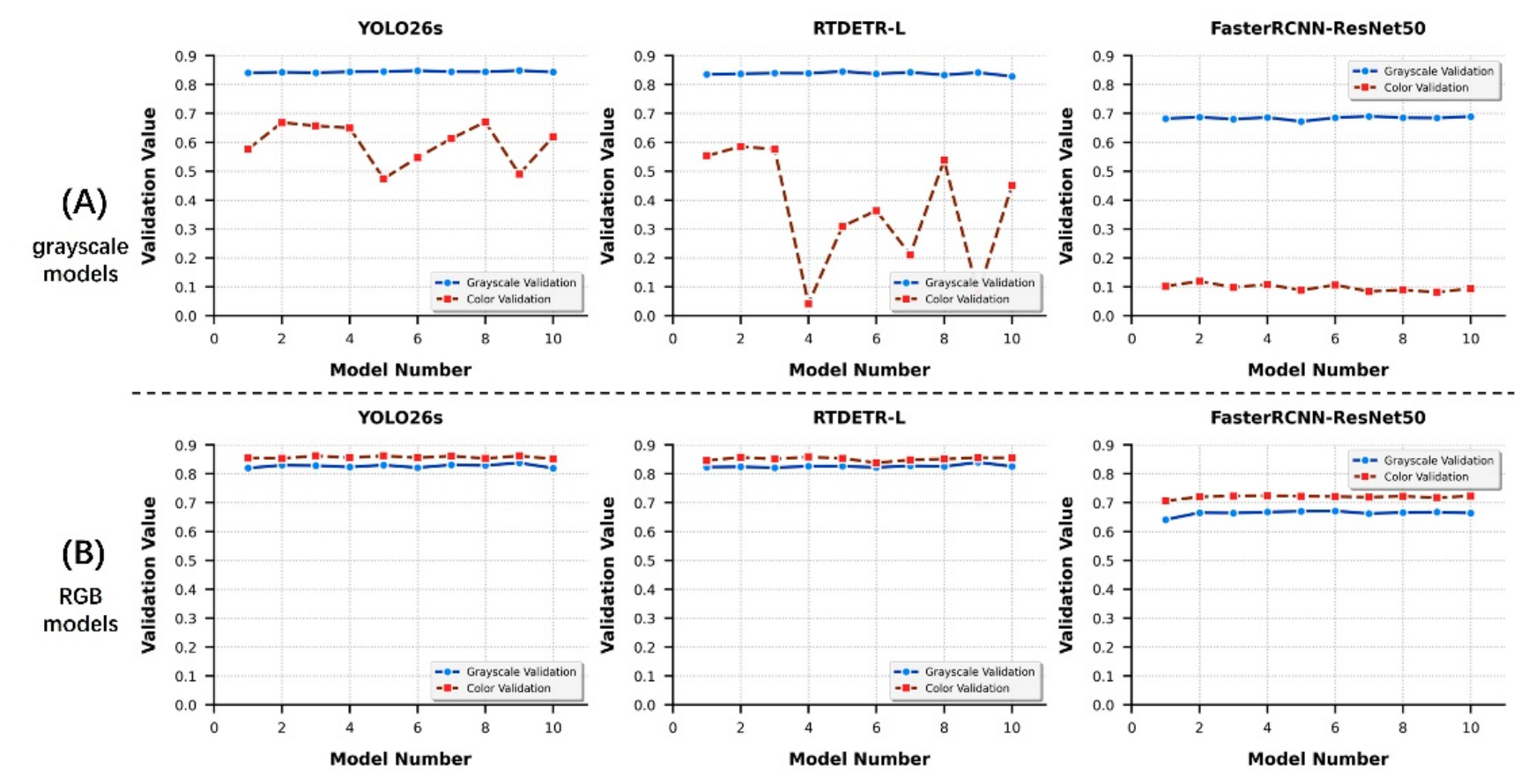
Figure 2.
Cross-Modal Validation and Comparison of Grayscale and Color Models. For each model (YOLOv5su, YOLOv8s, YOLO11s, and YOLO26s), 50 grayscale models and 50 RGB models are trained. The horizontal axis represents the N-th trained model, while the vertical axis represents the validation performance. The blue and red curves denote validation results on grayscale and RGB datasets, respectively. Region (A) on the left corresponds to cross-modal validation results of grayscale models, whereas region (B) on the right corresponds to cross-modal validation results of RGB models.
Figure 2.
Cross-Modal Validation and Comparison of Grayscale and Color Models. For each model (YOLOv5su, YOLOv8s, YOLO11s, and YOLO26s), 50 grayscale models and 50 RGB models are trained. The horizontal axis represents the N-th trained model, while the vertical axis represents the validation performance. The blue and red curves denote validation results on grayscale and RGB datasets, respectively. Region (A) on the left corresponds to cross-modal validation results of grayscale models, whereas region (B) on the right corresponds to cross-modal validation results of RGB models.
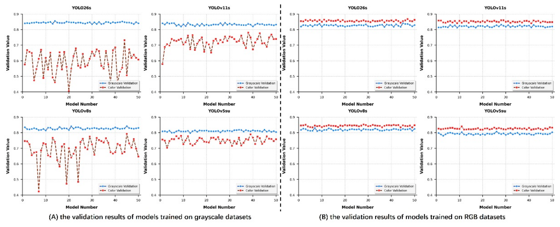
Figure 3.
Architecture of Layer 0 in YOLO Series.
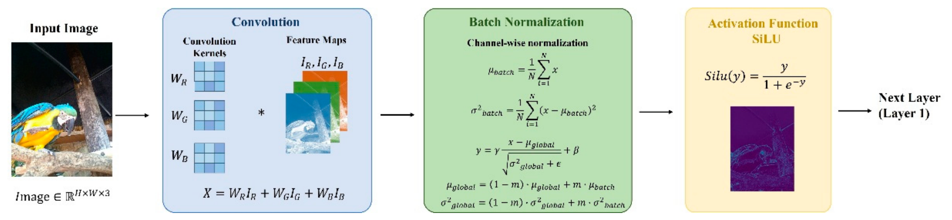
Figure 4.
Convolutional Kernels of Layer 0 in Pretrained YOLO26s. Figure 4 illustrates the distribution of pretrained weights for the convolutional kernels in the layer 0 module of the YOLO26s model. The x-axis represents the channel index, while the y-axis corresponds to the spatial positions within the convolutional kernel. Each point shows the sum of the weights across the three input dimensions at the same spatial location of the kernel (absolute value), with color encoding used to reflect the magnitude of the values.
Figure 4.
Convolutional Kernels of Layer 0 in Pretrained YOLO26s. Figure 4 illustrates the distribution of pretrained weights for the convolutional kernels in the layer 0 module of the YOLO26s model. The x-axis represents the channel index, while the y-axis corresponds to the spatial positions within the convolutional kernel. Each point shows the sum of the weights across the three input dimensions at the same spatial location of the kernel (absolute value), with color encoding used to reflect the magnitude of the values.
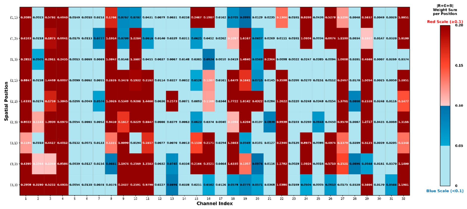
Figure 5.
Comparison of BN Layer Variance Between Grayscale and Color Models. The data in the figure are drawn from one grayscale model and one RGB model selected from each of YOLOv5su, YOLOv8s, YOLO11s, and YOLO26s as representative examples. In each subplot, the x-axis corresponds to the 32 channel indices of layer 0 in the YOLO series, and the y-axis represents the magnitude of the variance in the batch normalization (BN) layer for each channel. The red curve indicates the RGB model, while the blue curve represents the grayscale model.
Figure 5.
Comparison of BN Layer Variance Between Grayscale and Color Models. The data in the figure are drawn from one grayscale model and one RGB model selected from each of YOLOv5su, YOLOv8s, YOLO11s, and YOLO26s as representative examples. In each subplot, the x-axis corresponds to the 32 channel indices of layer 0 in the YOLO series, and the y-axis represents the magnitude of the variance in the batch normalization (BN) layer for each channel. The red curve indicates the RGB model, while the blue curve represents the grayscale model.
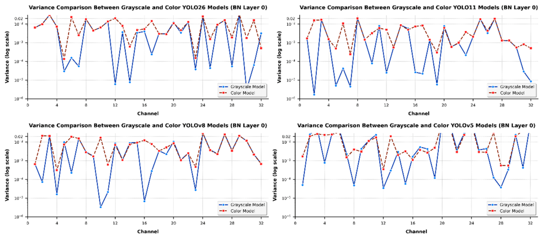
Figure 6.
Chromatic–Luminance Channel Distribution in Models. The figure illustrates the luminance–chromatic channel distributions for four YOLO model variants. The left column corresponds to channels in the grayscale models, while the right column corresponds to channels in the RGB models. The horizontal axis denotes the channel index of the first layer (layer 0), and the vertical axis represents the ColorScore values.
Figure 6.
Chromatic–Luminance Channel Distribution in Models. The figure illustrates the luminance–chromatic channel distributions for four YOLO model variants. The left column corresponds to channels in the grayscale models, while the right column corresponds to channels in the RGB models. The horizontal axis denotes the channel index of the first layer (layer 0), and the vertical axis represents the ColorScore values.
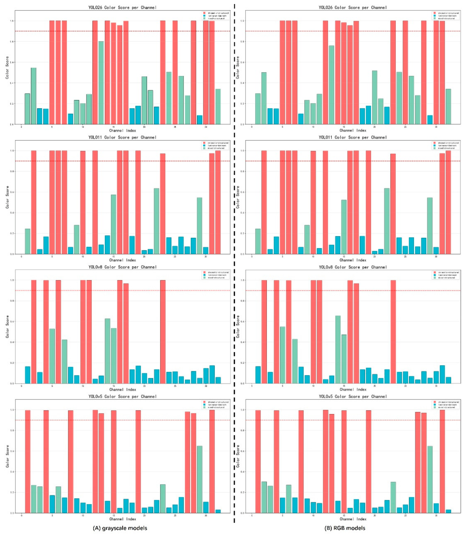
Figure 7.
Validation Results of Chromatic-Sensitivity Regularization.
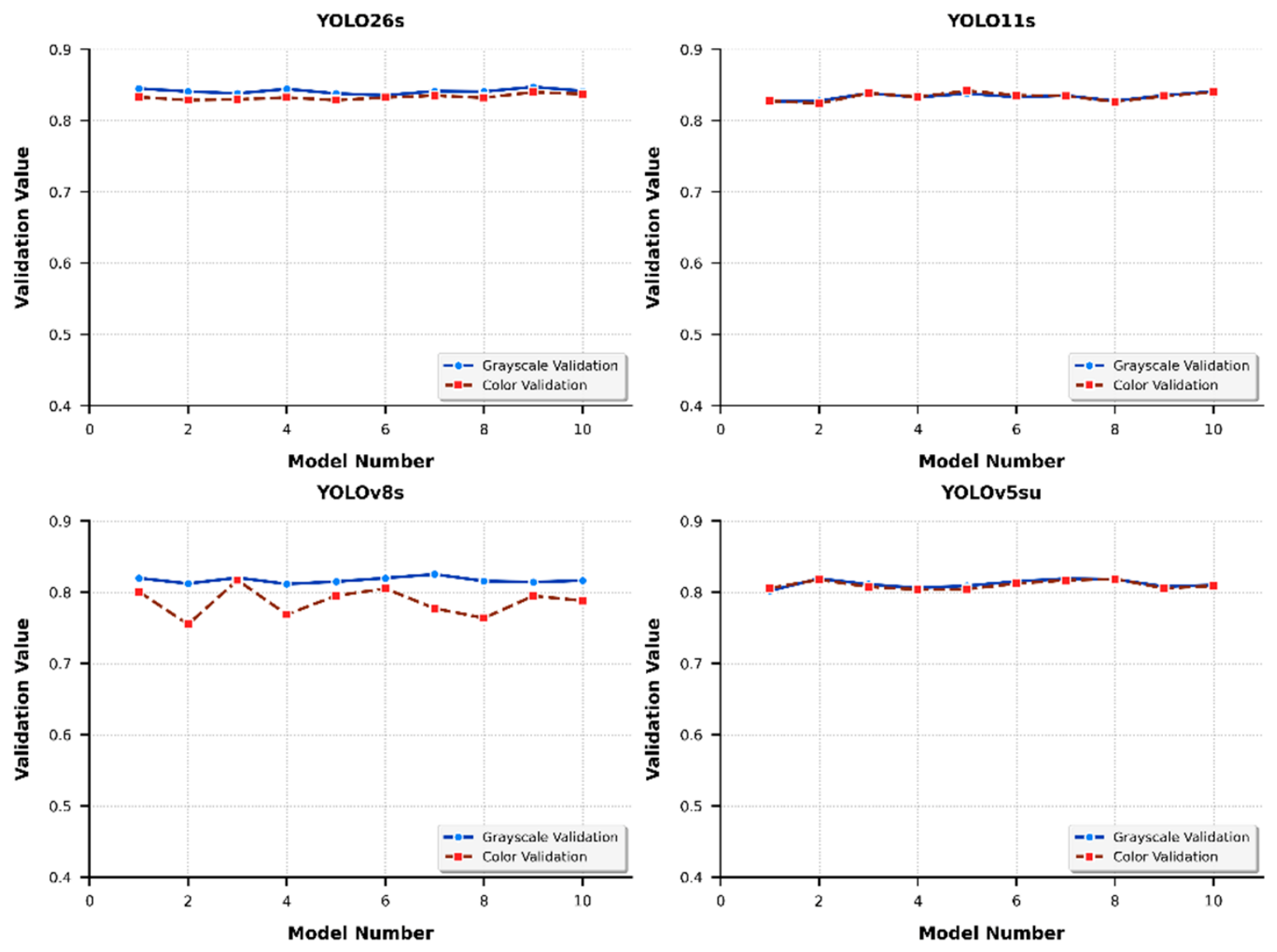
Figure 8.
Channel-wise ColorScore Distribution After Chromatic-Sensitivity Regularization.
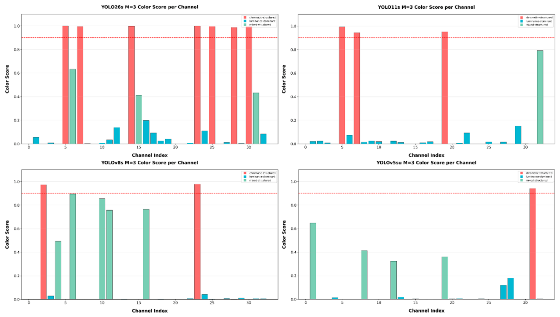
Figure 9.
Generalizability Validation of Chromatic Sensitivity Regularization.
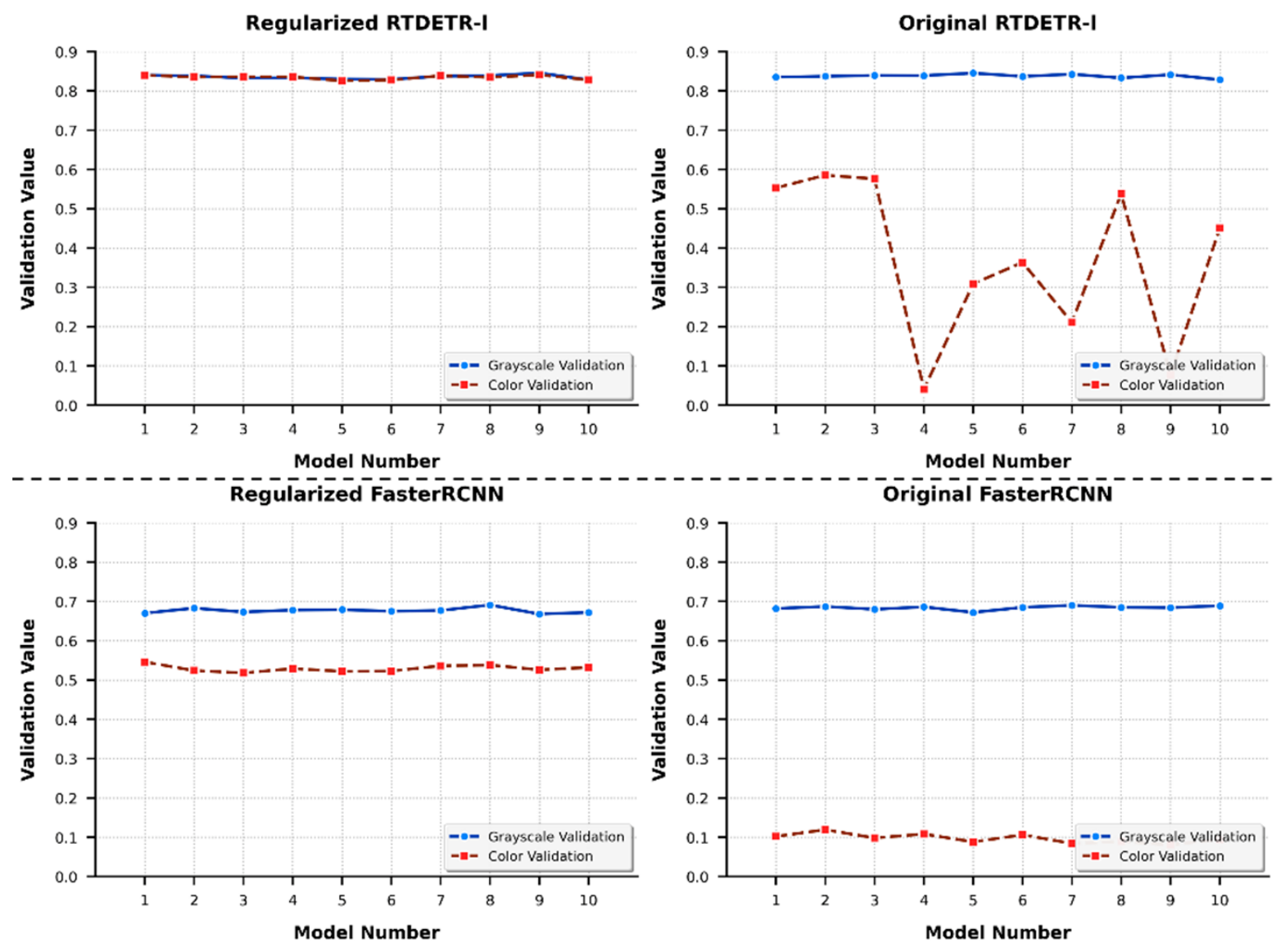
Table 1.
Summary of Experimental Results on Color Sensitivity Regularization.
| Parameter Settings | Model mAP50 Value | |||||||
| YOLO26s | YOLO11s | YOLOv8s | YOLOv5su | |||||
| Gray | Color | Gray | Color | Gray | Color | Gray | Color | |
| Baseline | 0.8450.004 | 0.5920.070 | 0.8330.006 | 0.7220.030 | 0.8270.006 | 0.6920.070 | 0.8100.005 | 0.7510.020 |
| 0.8410.004 | 0.8330.004 | 0.8340.005 | 0.8340.006 | 0.8170.004 | 0.7710.035 | 0.8110.006 | 0.8100.006 | |
| 0.8400.005 | 0.8330.004 | 0.8300.006 | 0.8320.004 | 0.8280.006 | 0.6650.133 | 0.8130.004 | 0.8030.008 | |
| 0.8380.005 | 0.8290.006 | 0.8310.005 | 0.8300.008 | 0.8290.005 | 0.6620.14 | 0.8140.005 | 0.7850.026 | |
| 18 | 0.8420.004 | 0.5550.045 | 0.8300.004 | 0.6610.055 | 0.831<!-- MathType@Translator@5@5@MathML2 (no namespace).tdl@MathML 2.0 (no namespace)@ -->0.005 | 0.4680.156 | 0.8100.005 | 0.5670.018 |
| 24 | 0.8440.001 | 0.4280.035 | 0.8320.005 | 0.4920.053 | 0.8300.006 | 0.3780.09 | 0.8070.004 | 0.4050.043 |
Table 2.
Summary of Experimental Results for Chromatic Sensitivity Regularization on RGB Models.
| Parameter Settings | Model mAP50 Value | |||||||
| YOLO26s | YOLO11s | YOLO26s | YOLOv5su | |||||
| Gray | Color | Gray | Color | Gray | Color | Gray | Color | |
| Baseline | 0.8270.006 | 0.8560.005 | 0.8210.005 | 0.8510.005 | 0.8190.005 | 0.8440.07 | 0.7930.005 | 0.8260.004 |
| 0.8250.006 | 0.8530.004 | 0.8230.004 | 0.8530.003 | 0.8200.004 | 0.8460.035 | 0.7960.004 | 0.8300.007 | |
| 24 | 0.8220.006 | 0.8520.006 | 0.8200.004 | 0.8540.004 | 0.8160.004 | 0.8410.005 | 0.7940.004 | 0.8260.004 |
Disclaimer/Publisher’s Note: The statements, opinions and data contained in all publications are solely those of the individual author(s) and contributor(s) and not of MDPI and/or the editor(s). MDPI and/or the editor(s) disclaim responsibility for any injury to people or property resulting from any ideas, methods, instructions or products referred to in the content. |
© 2026 by the authors. Licensee MDPI, Basel, Switzerland. This article is an open access article distributed under the terms and conditions of the Creative Commons Attribution (CC BY) license (http://creativecommons.org/licenses/by/4.0/).
Copyright: This open access article is published under a Creative Commons CC BY 4.0 license, which permit the free download, distribution, and reuse, provided that the author and preprint are cited in any reuse.


