

Submitted:
02 August 2026
Posted:
04 August 2026
You are already at the latest version
Abstract
Chronic and acute wounds are a significant and increasing burden on health care systems worldwide. A key step in ensuring timely and evidence-based treatment planning and intervention is accurate, automated wound-type classification. Previous deep learning-based methods for wound classification have been mainly based on alone-employed convolutional image encoders or simple late-fusion methods combining image and location features. The approaches are not well explained and are not robust over a range of morphologically equivalent wound types. In this work, we introduce a multimodal, spatially-aware Graph Neural Network-Concept Bottleneck Model (GNN-CBM) framework. This architecture offers a combined reasoning about the appearance of the wound images and the context of the anatomical location, and provides an exposure of a bottleneck of latent clinical prototypes before final classification. We systematically compared the seven backbone architectures used in the visual encoding stage of the framework, such as CNNs (ResNet-50, EfficientNet-B0, EfficientNetV2-S, ConvNeXt-Tiny, DenseNet-121) and Vision Transformers (ViT-Base, Swin-Tiny) on the AZH Wound and Vascular Center dataset (Milwaukee, WI), which includes N = 311 unique patients and an augmented working set of 830 image-location pairs. In order to avoid data leakage, patient identifiers were used as grouping variable in a 5-fold stratified group cross-validation scheme, ensuring that patient images are not contained in more than one fold. Overall, Swin-Tiny outperforms the other backbones with the highest accuracy (0.809 ± 0.014), macro-F1 (0.805 ± 0.016) and mean AUC (0.954). Adjusted McNemar's testing (Bonferroni corrected across 6 comparisons) returned that Swin-Tiny performed significantly better than five of the six other backbones, except ConvNeXt-Tiny, which is not significant. An ablation study of the proposed Domain-Constrained Spatial Penalty Loss revealed that when the anatomical penalty term was removed, macro-F1 scores dropped from 0.805 to 0.792 for the best model, indicating the impact of the spatial-plausibility constraint. We discuss the mathematical formulation of our framework, the anatomical graph construction and its density statistics, the implications of unsupervised concept bottlenecks on real interpretability, hardware efficiency and highlight the importance of external, multi-center validation prior to clinical deployment.
Keywords:
wound classification
; multimodal deep learning
; graph neural network
; concept bottleneck model
; AZH dataset
; medical image analysis
; explainable AI
1. Introduction
1.1. The Clinical Burden of Chronic and Acute Wounds
Tens of millions of patients globally suffer from chronic and complex acute wounds, such as diabetic foot ulcers, pressure wounds, surgical wound infections and venous leg ulcers. Their association with significant morbidity, longer hospital stays, increased risk of systemic infection, and reduced lower extremity amputation rates [1] is associated with significant morbidity. In the U.S. alone, direct medical costs for wound care are estimated to be in the tens of billions of dollars per year. The prevalence of comorbidities, including diabetes mellitus and peripheral vascular disease, is increasing and global populations are aging, and this will drive up the epidemiological burden of chronic wounds.
Correct primary wound diagnosis is the first step in the correct clinical triage of wounds. The pathophysiology, prognosis and first line dressing and debridement for diabetic, pressure, surgical and venous wounds is vastly different. For example, a venous leg ulcer will benefit from a multi-layer compression bandage that will apply compression - counteracting venous hypertension - while an arterial or severe diabetic ulcer with poor arterial supply will result in tissue necrosis and possible amputation when compression is applied. Therefore, the misclassification at intake can result in the incorrect management of these patients, slower recovery, and poor clinical outcomes.
However, as it stands, there are certain limitations with the current automated diagnostic systems. However, at present the diagnosis of wounds is very subjective and heavily dependent on the experience and visual heuristic of specialists in wound care. In recent years, deep convolutional neural networks (CNNs) and Vision Transformers (ViTs) have become prevalent technologies for automated analysis of medical images, owing to their ability to extract discriminative texture, color and morphological characteristics directly from the pixels of the image [2,3,4,5].
Nevertheless, using typical single-modality vision models in wound classification have two drawbacks:
- Visual Ambiguity: The appearance of the wound is often not enough to make a reliable classification. A very important note is that diabetic and pressure wounds can have very similar appearances with particularly the presence of necrotic eschar, yellow sloughs and peri-wound erythema features. Even though the morphology is not always a primary criterion, the anatomical location of the wound is of major importance when making the diagnosis. A wound on the plantar surface of the foot is very likely to be diabetic, while a wound with a similar morphology over the sacrum or ischial tuberosity is almost certainly a pressure injury.
- Opaque Decision Making: Opaque decision making is a property of neural networks that are trained end-to-end for a multi-way softmax output. They are unable to explain why they are given a certain class. A black-box prediction is a hurdle to clinician trust, workflow integration and regulatory approval in high stakes clinical settings.
1.2. Motivation for Multimodal and Latent Prototype Architectures
The multimodal wound classifiers integrating image features and structured anatomical location information were explored in recent works to overcome visual ambiguity [6,7]. Although these early fusion strategies show that location context helps increase the accuracy, they usually represent location as a one-dimensional categorical vector or a simple learned embedding without considering the non-Euclidean relational structure of the human anatomy (e.g., adjacency, laterality, and proximity to bony prominences).
At the same time, there has been a need for explainable AI (XAI) in the healthcare industry, which resulted in the creation of Concept Bottleneck Models (CBMs) [8]. The black-box problem is resolved by introducing an intermediate layer of concepts between the visual encoder and final classifier in CBMs. Graph Neural Networks (GNNs) [9,10] present a very useful mathematical model to overcome the location-encoding problem, as anatomical relationships are naturally represented by message-passing over a given graph topology.
1.3. Contributions
In this paper, we bridge these two domains by introducing and evaluating a multimodal, spatially-aware Graph Neural Network-Concept Bottleneck Model (GNN-CBM) framework. The research combines structured spatial reasoning using graph convolutions and concept-bottleneck representation in the classification of wounds. Our specific contributions are as follows:
- We develop a deterministic anatomical location mapping pipeline that takes raw wound images and produces structured body location identifiers with spatial coverage of an expanded working set of 830 image-location pairs from unique patients of the AZH dataset. Patient identifiers were used directly as the grouping variable within a stratified group k-fold cross-validation scheme (via StratifiedGroupKFold), so that no patient contributed images to more than one fold, at either the initial train/test split or the cross-validation stage.
- We propose an architecture called GNN-CBM which combines a GNN with visual feature embedding while preserving the anatomical structure. This fused representation is further processed by a bottleneck of 32 end-to-end learned latent clinical prototypes.
- We evaluate seven visual backbones (classical CNNs: ResNet-50, DenseNet-121, and modernised architectures: ConvNeXt-Tiny, EfficientNetV2-S, and Vision Transformers: ViT-Base, Swin-Tiny) systematically using a strict 5-fold stratified group cross-validation protocol with full per-fold results presented for each architecture.
- We propose an epidemiologically motivated Domain-Constrained Spatial Penalty Loss for penalising unforeseen anatomical predictions when training the model and implement a dedicated ablation study by comparing the full model with an otherwise identical model but with an empirically set zero penalty weight to isolate the effect of the domain constraint.
- We perform comprehensive statistical validation (Bonferroni adjusted McNemar’s tests, calibration analysis using Expected Calibration Error) to measure differences across backbones, and to evaluate the compromises between architectural complexity, computational efficiency, and diagnostic accuracy.
2. Related Work
2.1. Deep Learning in Wound Image Analysis
Historically, in the field of wound care, deep learning has been applied to purely image-based segmentation, boundary delineation and classification. The few large, well-annotated wound datasets were unavailable for the early architectures, so Anisuzzaman et al. [6] were among the first to release the AZH and Medetec wound datasets to the machine learning community at-large. They showed that CNNs could work well on obvious cases of visual markers, but suffered from ambiguity on edge cases where tissue texture was not clear.
The more recent methods are using image preprocessing with more advanced techniques, such as discrete wavelet transforms and CLAHE-based image enhancement, and ensemble learning involving CNN and capsule networks Odame et al. [11]. In a similar fashion, Alhababi et al. [12] suggested a unified segmentation-and-classification framework, based on the idea that the introduction of the wound boundaries as regularization for the classification task. Light-weight detectors like YOLO11n are also benchmarked on AZH, focusing on the efficiency of the inference for point-of-care mobile applications for multi-way wound classification [13]. Although effective, these approaches are limited to the visual domain and fail to account for the fact that the clinical context is predictive of the origin of a wound (anatomical location).
2.2. Multimodal Fusion and Medical Foundation Models
To address the drawbacks of unimodal systems, Patel et al. Patel et al. [7] built upon the framework of Anisuzzaman et al. [6], adding the location data as a structured input with the image features using multi-layer perceptrons (MLPs). Their results showed that a minimal amount of data fusion, such as late-fusion of location data, can still make a significant difference in the diagnostic accuracy.
Transformer based architectures have also been used in this multimodal paradigm. Recently, a framework that coupled Vision Transformers (ViT) with location has been suggested using wavelet augmentation and complex cross-attention mechanisms [14]. However, these fusion strategies consider anatomical location as discrete categorical variables, where no attempt is made to take advantage of the topological relation between the various parts of the body. Moreover, although Medical Foundation Models provide very strong pre-trained representations, aligning the models to specific, location-specific dermatological tasks is often both time-consuming and labor-intensive.
2.3. Concept Bottleneck Models (CBMs) and Explainable AI
Transparency of deep learning models is a key challenge in health care. Standard post-hoc interpretability methods (e.g., Grad-CAM, saliency maps) identify important pixels but cannot provide clinically-relevant explanations of those pixels. There are models of interpretability that take a “by-design” approach, such as the Concept Bottleneck Models [8]. In a CBM, the network is given a set of concepts to predict, and it can only predict the last label from the predicted concepts.
Original CBMs necessitated time-consuming, dense annotation by humans for each concept in the training process; however, recent work has lessened this requirement. Some post-hoc CBMs [15] and visual-preference-enhanced CBMs [16] have been proposed to align the concepts with latent features without strict supervision, which was applied to skin lesion tasks by Kim et al. [17]. Moreover, Xu et al. [18] proposed a new model called Graph Concept Bottleneck Models, which demonstrated that latent concepts are not independent, and that they can be represented as a graph.
2.4. Graph Neural Networks in Anatomical Modeling
Graph Neural Networks (GNNs) [9,10] are especially designed for non-Euclidean structures. In the medical imaging field, GNNs have been applied for tissue topology modelling and vascular network modelling and anatomical adjacency modelling [19,20].
In such cases, the long-range dependencies in a chest radiograph analysis problem is tackled by the superpixel graph learning problem introduced by SPX-GNN [21]. MedGNN builds a graph over structural MRI patches to represent the geometric priors learned from brain lesions [22]. We believe our proposed framework is one of the first attempts to generate an explicit anatomical body-location graph, and combine the information from these message-passed representations with a visual encoder for wound classification.
3. Materials and Methods
3.1. Dataset Formulation and Cohort Characteristics
The dataset of AZH wound images was used, which was originally acquired within a continuous 2-year clinical period at the AZH Wound and Vascular Center in Milwaukee, WI [6]. The raw data consists of 830 clinical images of wounds that were obtained from different patients. The labels corresponding to the etiology of the images were assigned by board certified wound care specialists with the following main output classes: “Diabetic” (D), “Normal/Background” (N), “Pressure” (P), “Surgical” (S), and “Venous” (V). The class distribution is in line with the natural prevalence in a clinical environment in an outpatient vascular setting, which requires class-weighted loss functions for the optimization of the network. Figure 1 shows some examples of clinical samples for each of the five categories.
3.1.1. Dataset Partitioning and Leakage Prevention
One of the main challenges in medical machine learning is the presence of multiple images for the same patient from various visits or anatomical locations, which poses a significant data leakage challenge. To ensure robust evaluation, we carefully separated patients prior to any dataset separation, and separated patients throughout the model selection process. Concretely, patient identifiers were supplied as the groups argument to scikit-learn’s StratifiedGroupKFold, which was used both (i) to derive the initial held-out test partition and (ii) to construct the five cross-validation folds used for model selection within the training partition. This ensures that the image data for a particular patient will not be included in both the training and the validation/Test fold. These partitioning levels were patient-level, and were only then followed by data augmentation methods, creating a total of image-location pairs (). The images are all in RGB format, , and were originally between 320x240 and 700x525 pixels.
3.2. Deterministic Anatomical Location Mapping
A crucial aspect of our spatial GNN module is that each image comes with a valid spatial prior. We devised a deterministic mapping pipeline working with the metadata and clinical logs to assign a structured identifier to the images .
3.2.1. Clinical Annotation and Agreement
A standard anatomical atlas was used to create the discrete series of location identifiers. Two wound care clinicians divided the body into a grid of discrete anatomical regions. The inter-rater reliability of assigning retrospective images to these 400 regions was high (Cohen’s Kappa ). Any differences were addressed through consensus. The automated mapping pipeline was able to map 100% of the working set without any “null” locations appearing in the network that would inhibit the fusion.
3.2.2. The Density and Graph Topology
The anatomical graph has nodes, directed edge entries (for 760 unique undirected edges) and is connected by only orthogonal (non-diagonal) edges. This results in a graph density of about 0.95% of all possible node pairs, and a mean node degree of 3.80 (with 4 corner nodes having degree 2, edge nodes degree 3, and interior nodes degree 4). The edges are unweighted and are binary. We chose a 4-connected (non-diagonal) topology rather than an 8-connected (diagonal-inclusive) topology to ensure that the receptive field of each layer of the GCN is anatomically-conservative, as we discuss in Section 5.5 below.
3.3. Mathematical Formulation of the GNN-CBM Architecture
The proposed multimodal framework consists of three different computation stages: Visual Encoding, Spatial Graph Message Passing, and Concept Bottleneck Fusion.
3.3.1. Visual Feature Extraction (Stage 1)
Suppose that an image of an input wound is represented as , where H and W are dimensions and the number 3 signifies the three RGB color channels. Apply a deep visual backbone to process x with some parameters . We assessed seven different architectural paradigms that cover the current state of the art in computer vision to define a comprehensive benchmark.
- EfficientNet-B0 [4] and EfficientNetV2-S: Compound scaling and training aware neural architecture search.
- ConvNeXt-Tiny [5]: Macroscopic design (such as depthwise convolution) inspired by modern transformer models ().
- ViT-Base and Swin-Tiny: Pure self-attention and shifted-window hierarchical Vision Transformers.
The global-average-pooled (GAP) output of the visual encoder is a dense 1D visual embedding , where is the dimensionality of the visual embedding.
3.3.2. Spatial Graph Message Passing (Stage 2)
The structure of the human body is modelled by an anatomical location graph , in which the vertex set represents the distinct anatomical regions throughout the body, with the links connecting them according to Section 3.2.2. The structural proxy used for anatomical surface connectivity was a 2D grid adjacency schema, but complex 3D meshes were ideal for human anatomy.
Let be the adjacency matrix of . Two layers of Message Passing are performed in the Graph Convolutional Network (GCN) module to pass the topological information between neighboring anatomical regions:
The node feature matrix at layer l is denoted as while the adjacency matrix with self-loops is denoted as . The degree matrix of the adjacency matrix is denoted as , the weight matrix is and the ReLU activation function is . The spatial embedding for an image is directly obtained from the final GNN layer for an image with a location index .
where .
3.3.3. Concept Bottleneck Fusion and Final Classification (Stage 3 )
The visual embedding and the context-aware spatial embedding are fused by simply concatenating them together. Concatenated vector is projected to lower dimensional latent space:
and where the ’||’ is for concatenation.
The is fed into a Concept Bottleneck Layer with discrete concepts, to ensure explainability. The dense annotations of concepts required are too costly to be made manually, so they are learned end-to-end without any explicit clinical supervision, instead of being strictly grounded semantic labels. The concept activation probabilities are calculated as:
Finally, a linear classification head maps the concept probabilities to the last etiology logits (with classes).
The optional residual connection bypasses the bottleneck to prevent early training dynamics from getting too unstable.
3.4. Domain-Constrained Spatial Penalty Loss
Standard Cross-Entropy () assumes that all misclassifications are equally important. However, it is unlikely to be biologically possible to predict a venous ulcer on the face. We propose a customized Domain-Constrained Spatial Penalty Loss () which includes a pre-defined penalty matrix .
This matrix was built with the help of two senior wound care physicians in collaboration with established epidemiology data, and the values were assigned continuously between 0 and 1, depending on the anatomical region and class (e.g., for a venous-ulcer prediction over a node that is a head/neck, and for a node that is lower-limb and does not have any known contraindication). A venous ulcer on an anatomical node in the face is assigned while a pressure ulcer on a high risk anatomical node of the sacral region is assigned . The loss function function that is optimised during training is:
We use the inverse class frequencies to pre-compute weights for the full model , to compensate for imbalanced datasets.
3.5. Experimental Procedure and Training Dynamics
To control the model selection and evaluation, a 5-fold stratified group cross-validation scheme was used, where the grouping variable was the patient identifier (Section 3.1). Stratification allowed the patient-grouping constraint to be satisfied and maintained the same proportions of classes in each training and validation split. The full list of all hyperparameters needed to replicate this study is found in Table 1.
3.6. Statistical Evaluation Metrics
The accuracy, sensitivity (recall), precision, macro-F1 score and area under the Receiver Operating Characteristic Curve (AUC, one-vs-rest, macro-averaged) were used to quantify model performance. The Expected Calibration Error (ECE) over 10 equally sized confidence bins was also used to evaluate the calibration. Standard deviation (SD) of the five fold-level scores were used to obtain the 95 percent confidence intervals (CI) which were reported along with the fold means: .
To determine if there are statistical differences in architecture, we ran McNemar’s Test [23] on the paired nominal predictions of the best architecture compared to each other architecture on the held-out test set with continuity correction applied. Since multiple pairwise comparisons were made against the reference model, a Bonferroni correction was applied to the six comparisons, resulting in an adjusted significance threshold of .
4. Results
4.1. Cross-Validation Dynamics and Stability
Table 2 shows the full fold-by-fold test accuracy for all seven backbones with the full GNN-CBM structure (); there are no folds that are left out. Swin-Tiny presented the highest mean accuracy and the smallest difference between the first and last fold, ranging from 0.799 to 0.828 across folds. Next, the ConvNeXt-Tiny architecture was the second most stable one. ResNet-50 and EfficientNet-B0 had significantly larger variations of accuracy within the folds (accuracy ranges from 0.656 to 0.751 and 0.641 to 0.727, respectively), suggesting greater sensitivity to the patient mix in each training fold. This variation can be directly observed in Figure 2 as a boxplot of macro-F1 scores for each of the patient-level folds for each backbone.
4.2. Aggregate Clinical Metrics and Architectural Benchmarking
Table 3 shows the aggregated clinical performance, calibration and efficiency results for all seven evaluated architectures. Swin-Tiny achieved the best accuracy of and macro-F1 of as well as mean AUC of which is better than other architectures, achieving competitive calibration (ECE ), and moderate inference cost. ConvNeXt-Tiny and ViT-Base were competitive in terms of accuracy and macro-F1, despite ViT-Base being significantly larger in terms of inference latency and number of parameters, and, importantly, not exhibiting the convergence problems found in previous internal runs of this study when patient-grouped cross-validation and the full training protocol were applied across all backbones.
The per-class ROC curves for Swin-Tiny (the best-performing model) on the held-out test set are shown in Figure 3. As shown in Section 5.2, there was a high visual and spatial overlap between the Pressure (P) class and the diabetic wound class, which is reflected by the comparatively weaker discrimination for the P class, although it remains acceptable (AUC ), as well as the Normal/Background (N) class (AUC ) and the Venous (V) class (AUC ).
4.3. Per-Class Performance of the Top Model
Table 4 shows the per-class precision, recall and F1 scores of Swin-Tiny. The Normal/Background class was classified almost perfectly (F1 ), and the Pressure class was the most challenging (F1 ), which was mainly due to the misclassification of Normal class with the Diabetic and Venous classes as shown in the normalized confusion matrices of Figure 4.
4.4. Statistical Significance (Adjusted McNemar’s Test)
Pairwise McNemar’s tests (with continuity correction) were conducted between the best-performing Swin-Tiny and all other six backbones. For six comparisons the Bonferroni correction gives an adjusted alpha level of . Swin-Tiny markedly outperforms ResNet-50, EfficientNet-B0, EfficientNetV2-S and DenseNet-121 as indicated in the Table 5. The difference relative to ConvNeXt-Tiny and ViT-Base was not statistically significant after correction, suggesting that, with the current number of images in the dataset, Swin-Tiny is approximately equivalent in function to these two architectures.
4.4.1. Ablation of the Domain-Constrained Spatial Penalty Loss
To evaluate the impact of the proposed spatial penalty term, the best-performing backbone (Swin-Tiny) was retrained without adding the spatial penalty term (setting to zero) while other algebraic, architectural, and training parameters remained the same. The resulting fold-averaged macro-F1 is shown in Table 6. The absolute decrease in macro-F1 from 0.805 (full model, ) to 0.792 (ablated model, ), which is 1.33 percentage points, suggests that in addition to what the GNN spatial embedding can achieve, penalizing anatomically implausible predictions offers a measurable, albeit small, advantage. We observe that the validation loss of the ablated model is also significantly smaller (around 0.6 vs. around 0.9 for the full model) as the penalty term is part of the optimized loss function and is not directly comparable between the two models; it is not surprising that the test-set macro-F1 remains the relevant metric for the comparison.
4.5. Concept Bottleneck Activations
For a representative set of test images fed into the best Swin-Tiny model, (top) the strength of the activation of the 32 latent concepts, labeled with the true and predicted classes of each sample, and (bottom) the learned linear weights that map each concept to each of the 5 output classes. Some prototype numbers (such as C16, C27, C32) have consistently high activation over the Diabetic-labeled samples, and similarly high weights towards the Diabetic class, indicating that they have specialized on aspects of the samples that are repeatedly related to diabetic wounds, despite being learned without semantic supervision. This behavior is not necessarily interpreted clinically without foundation and we refer to it as structural transparency (as discussed in Section 5.3).
5. Discussion
5.1. Architectural Inductive Biases in Multimodal Pipelines
Empirical consequences throughout this study yield insightful understanding of the interaction of different visual inductive biases with downstream non-Euclidean graph fusions. The observed hierarchy, that is, the performance of Swin-Tiny and ConvNeXt-Tiny exceeds that of ResNet-50 and EfficientNet-B0, and the performance of Swin-Tiny is superior to ConvNeXt-Tiny, indicates that the choices of the visual modality have cascading effects on the multimodal bottleneck layer.
Swin-Tiny’s strong performance corroborates its hierarchical, shifted-window self-attention design, which enables the network to learn local texture (fine-grained slough, granulation, and erythema patterns) and longer-range contextual dependencies (overall shape of the wound boundary and the surrounding peri-wound tissue), without the quadratic attention cost of a full ViT. Unlike the pure ViT, where self-attention is calculated across the entire image, Swin-Tiny only uses local windows and asks to progressively shift and merge those windows across stages, essentially serving as a helpful inductive bias on this dataset (830 image-location pairs from 311 patients). This is confirmed by our findings: Without this windowed locality bias, ViT-Base needed the full training schedule and patient-grouped cross validation employed throughout this revision to achieve competitive accuracy (0.778) and macro-F1 (0.771) performance metrics, while still being outperformed by Swin-Tiny on all aggregation metrics, with an error rate of around 2.5× and parameter count of around 3×.
Combined with the GNN-CBM fusion stage, ConvNeXt-Tiny was also found to be highly competitive with Swin-Tiny, with the gap not being statistically significant following Bonferroni correction (Table 5). Both modernized architectures (convolutional and attention-based) learned comparable useful representations for this task. Not only that, but DenseNet-121 performed well for a network with such small a parameter budget, which aligns with the notion that dense feature concatenation preserves granular low-level textural gradients (e.g., subtle colour changes representing tissue ischaemia) that can otherwise be lost in deeper networks trained on smaller medical datasets.
5.2. The Role of Graph Neural Networks in Anatomical Reasoning
Designing a Graph Neural Network to encode anatomical locations is a major methodological shift from previous wound classification systems that relied on more typical categorical encoding methods. In previous multimodal approaches, the body locations were just treated as separate and independent variables, with no intrinsic mathematical relationship between a wound on the “calf’ and a wound on the “ankle’ until the network was trained to find them.
The human body, however, is another continuous topological surface, subject to strict rules of biology. Venous hypertension occurs along specific pathways of the veins, pressure injuries occur over weight-bearing bony prominence. Our GNN module makes the network acknowledge these spatial facts by building an explicit mathematical graph with a mean node degree of 3.80 (Section 3.2.2). In the message-passing phase, the node connected to a given anatomical region collects information from neighbouring nodes in order to incorporate the spatial prior into the latent space of the network.
Pressure (P) remained the most difficult class to discriminate (F1 ; ROC AUC ; the lowest of all the classes) and the confusion matrices in Figure 4 reveal that pressure (P) was most likely to be confused with Venous (V) and Diabetic (D) across almost all backbones. This is anatomically feasible: patients with multiple comorbidities may have pressure, venous, and diabetic wounds in overlapping areas of the lower body and existing grid-graphs of size do not represent finer distinctions like proximity to bony prominences and weight-bearing status, which could help disambiguate these cases. The ablation in Section 4.4.1 demonstrates that the domain-constrained spatial penalty loss is a worthwhile addition to the implicit spatial encoding of the GNN (macro-F1 vs. without the penalty).
5.3. The Nature of Interpretability in Unsupervised Concept Bottlenecks
One of the key issues to discuss is the nature of the “interpretability” that our Concept Bottleneck Layer provides. High accuracy can only be obtained in standard end-to-end deep learning, at the price of losing transparency, which makes it not attractive to physicians. CBMs try to solve this problem by “pushing” the reasoning of the network into an intermediate concept space.
For this reason, we assume the concepts in our framework are learned end-to-end without any explicit clinical labels (i.e., instead of being called C1, C2, …, C32 they simply exist as concepts). Thus, these nodes are not actual semantic concepts but rather are latent clinical prototypes. They are grouped around the definition of visual and spatial properties (Figure 5), but it is too early to state that they are absolutely clinically interpretable. In order to be unambiguously interpretable, a CBM must be capable of being explicitly stated by a clinician as “Concept 4 unequivocally represents maceration.”. While unsupervised CBMs provide structural transparency (i.e., the model’s reasoning passes through this bottleneck and it can be examined and audited), they lack true semantic explainability without the help of post-hoc concept alignment using expert labeling or Vision-Language Models (VLMs). In this study, we consistently employ specific vocabulary instead of strongly worded clinical interpretability.
5.4. Clinical Workflow Implications and Hardware Efficiency
The operationalization of this framework holds measurable potential for clinical workflows. In an outpatient wound care clinic, a clinician could capture an image of a wound using a standard mobile device, tapping the anatomical location on a digital body map interface. The GNN-CBM would then process these inputs in a few milliseconds of model inference time.
From a hardware deployment perspective, the choice of architecture is a meaningful trade-off. As shown in Table 3, Swin-Tiny achieves the best accuracy and macro-F1 with a moderate footprint (28.3M parameters, 4.5 GFLOPs, 5.15 ms mean inference time), making it a reasonable default for server-side or workstation deployment. For more constrained edge deployment (e.g., a nurse’s tablet), DenseNet-121 offers a favorable trade-off, reaching macro-F1 of 0.734 with only 8.0M parameters, 2.9 GFLOPs, and the lowest inference latency among the mid-tier performers (3.25 ms), at a modest cost in accuracy relative to Swin-Tiny. ViT-Base, in contrast, is difficult to justify for deployment: it requires 86.6M parameters and 17.6 GFLOPs — roughly 3× and 4× those of Swin-Tiny, respectively — for statistically indistinguishable performance.
5.5. Limitations and the Critical Need for External Validation
The results of the experiments confirm the effectiveness of the GNN-CBM architecture, but there are some relevant limitations that set the course for future studies.
Lack of external validation: This is the largest weakness of this study as it is a single dataset and single institution. The AZH data set is meticulously maintained, and in this revision, patient-level separation is verified at each cross-validation iteration but the cross-validation performed on a single cohort is only internal validation and not external generalizability. The pictures represent the conditions and equipment that are typical to a particular clinic in Wisconsin, and reflect the lighting schedules, equipment and population distribution that are typical to that clinic. Therefore external validation in fully independent, multi-centre cohorts (cross-hospital validation) is a crucial next step in order to be able to make claims of more general clinical robustness. We see the one biggest priority area for future contributions to medical AI journals as the requirement for temporal or hospital independent validation, to avoid learning site-specific artifacts from the algorithms.
Anatomical graph construction simplifications: For this study the anatomical graph was simplified and constructed using a generalized 4 connected 2D grid adjacency schema with 400 nodes (mean degree 3.80, Section 3.2.2). Although this serves as a good illustration of the benefits of topological message-passing, it is also a caricature of true human anatomy; a 2D grid is hard to use for explaining the curvature of limbs, wrap-around adjacency (e.g., the two sides of a limb), or the exact closeness of vascular and bony structures that still creates some ambiguity between the Pressure, Diabetic, and Venous classes, as explained in Section 5.2.
Ethical and Demographic Fairness: The dataset does not have explicit metadata on patient demographics (e.g., Fitzpatrick skin type, age, sex). Algorithms for dermatological diagnosis often perform differently depending on skin tone, and may not be able to detect erythema on darker skin. Not testing the model for its demographic fairness is a serious ethical concern.
5.6. Future Directions
The current 2D grid proxy needs to be replaced by mathematically precise 3D anatomical meshes (i.e. SMPL human body model, formal anatomical atlases) in future versions of this model. Constructing a 3D mesh would enable the GNN to estimate accurate geodesic distances on the surface of the skin, which could further reduce this residual ambiguity between neighbouring classes that are anatomically adjacent like Pressure and Venous, and improve the accuracy of the spatial context embedding.
Moreover, future research needs to be based on grounding the latents with Medical Foundation Models or Vision-Language Models (VLM) like MedSAM or CLIP-based VLM. The framework will shift from being a purely structural transparency toward a truly clinically interpretable framework by aligning the latent space with the vocabulary actively used by physicians, such as “erythema,” “granulation,” and “slough.” Lastly, the external validity of the data needs to be established through prospective, multi-site data collection before clinical use.
6. Conclusion
In this research, we introduced a spatially-aware Graph Neural Network–Concept Bottleneck Model (GNN-CBM) that is able to accurately classify chronic and acute wounds. We benchmarked seven widely-used visual architectures, and found that Swin-Tiny was the best visual encoder for this multimodal classification task, with accuracy and macro-F1 ; ConvNeXt-Tiny and ViT-Base were statistically indistinguishable. Our deterministic anatomical mapping pipeline guaranteed that our GNN module can provide a structural context for every prediction with of spatial coverage, and the proposed Domain-Constrained Spatial Penalty Loss was shown to be an effective way to improve the GNN’s prediction performance over its implicit spatial encoding (macro-F1 vs. ), through a dedicated ablation study. The results are further addressed in extensive statistical tests and calibration analysis. We refer to this as a Concept Bottleneck Layer and, as it currently stands, it is far from clinically interpretable, and for this or any other trained framework to be of use in clinical triage, the need for external multi-center validation is paramount.
The AZH wound image dataset and associated preprocessing code utilized in this study are available in the public repository at https://github.com/uwm-bigdata/wound-classification-using-images-and-locations, subject to the ethical terms of use of the original dataset.
This manuscript was not prepared with the aid of AI writing or language tools. The authors shall be solely responsible for any errors of fact or omissions in or resulting from the use of this information.
Author Contributions
All four authors contributed equally to the Introduction, Related works, Materials and Methods, Results, Discussion, and drafting of this work. All authors have read and agreed to the published version of the manuscript.
Conflicts of Interest
The authors declare that the research was conducted in the absence of commercial or financial relationships that could be construed as a potential conflict of interest.
References
- Sen, C.K. Human wound and its burden: updated 2020 compendium of estimates. 2021. [Google Scholar] [CrossRef] [PubMed]
- He, K.; Zhang, X.; Ren, S.; Sun, J. Deep residual learning for image recognition. In Proceedings of the Proceedings of the IEEE Conference on Computer Vision and Pattern Recognition (CVPR), 2016; pp. 770–778. [Google Scholar]
- Huang, G.; Liu, Z.; Van Der Maaten, L.; Weinberger, K.Q. Densely connected convolutional networks. In Proceedings of the Proceedings of the IEEE Conference on Computer Vision and Pattern Recognition (CVPR), 2017; pp. 4700–4708. [Google Scholar]
- Tan, M.; Le, Q. EfficientNet: Rethinking model scaling for convolutional neural networks. In Proceedings of the International Conference on Machine Learning (ICML), 2019; pp. 6105–6114. [Google Scholar]
- Liu, Z.; Mao, H.; Wu, C.Y.; Feichtenhofer, C.; Darrell, T.; Xie, S. A ConvNet for the 2020s. In Proceedings of the Proceedings of the IEEE/CVF Conference on Computer Vision and Pattern Recognition (CVPR), 2022; pp. 11976–11986. [Google Scholar]
- Anisuzzaman, D.M.; Patel, Y.; Rostami, B.; Niezgoda, J.; Gopalakrishnan, S.; Yu, Z. Multi-modal wound classification using wound image and location by deep neural network. Sci. Rep. 2022, 12, 20057. [Google Scholar] [CrossRef] [PubMed]
- Patel, Y.; Shi, H.; Rostami, B.; Niezgoda, J.; Gopalakrishnan, S.; Yu, Z. Integrated image and location analysis for wound classification: a deep learning approach. Sci. Rep. 2024, 14, 7043. [Google Scholar] [CrossRef] [PubMed]
- Koh, P.W.; Nguyen, T.; Tang, Y.S.; Mussmann, S.; Pierson, E.; Kim, B.; Liang, P. Concept bottleneck models. Proc. Proc. 37th Int. Conf. Mach. Learn. (ICML) 2020, Vol. 119, 5338–5348. [Google Scholar]
- Kipf, T.N.; Welling, M. Semi-supervised classification with graph convolutional networks. In Proceedings of the International Conference on Learning Representations (ICLR), 2017. [Google Scholar]
- Casanova, A. Graph attention networks. arXiv Mach. Learn. 2017. [Google Scholar]
- Odame, P.; Ahiamadzor, M.M.; Derkyi, N.K.B.; Boateng, K.A.; Sarfo-Acheampong, K.; Tchao, E.T.; Agbemenu, A.S.; Nunoo-Mensah, H.; Agyapong, D.A.Y.; Kponyo, J.J. Multi-wound classification: exploring image enhancement and deep learning techniques. Eng. Rep. 2025, 7, e70001. [Google Scholar] [CrossRef]
- Alhababi, M.; Auner, G.; Malik, H.; Aljasem, M.; Aldoulah, Z. Unified wound diagnostic framework for wound segmentation and classification. Mach. Learn. With Appl. 2025, 19, 100616. [Google Scholar] [CrossRef]
- Jeribi, F.; Siddiqa, A.; Kibriya, H.; Tahir, A.; Rana, N. Efficient wound classification using YOLO11n: a lightweight deep learning approach. Comput. Mater. Contin. 2025, 85, 955–982. [Google Scholar] [CrossRef]
- Mousa, R.; Matbooe, E.; Khojasteh, H.; Bengari, A.; Vahediahmar, M. Multi-modal wound classification using wound image and location by Xception and Gaussian Mixture Recurrent Neural Network (GMRNN). arXiv 2025, arXiv:2505.08086. [Google Scholar]
- Yuksekgonul, M.; Wang, M.; Zou, J. Post-hoc concept bottleneck models. In Proceedings of the International Conference on Learning Representations (ICLR), 2023. [Google Scholar]
- Wang, C.; Zhang, K.; Liu, Y.; He, Z.; Tao, X.; Zhou, S.K. Mvp-cbm: Multi-layer visual preference-enhanced concept bottleneck model for explainable medical image classification. arXiv 2025, arXiv:2506.12568. [Google Scholar]
- Kim, I.; et al. Concept bottleneck with visual concept filtering for explainable medical image classification. In Proceedings of the International Conference on Medical Image Computing and Computer-Assisted Intervention (MICCAI), 2023; pp. 225–233. [Google Scholar]
- Xu, H.; Weng, T.W.; Nguyen, L.M.; Ma, T. Graph concept bottleneck models. arXiv 2025, arXiv:2508.14255. [Google Scholar]
- Mienye, I.D.; Viriri, S. Graph Neural Networks in Medical Imaging: Methods, Applications and Future Directions. Information 2025, 16, 1051. [Google Scholar] [CrossRef]
- Jeribi, F.; Siddiqa, A.; Kibriya, H.; Tahir, A.; Rana, N. Efficient wound classification using YOLO11n: a lightweight deep learning approach. Comput. Mater. Contin. 2025, 85, 955–982. [Google Scholar] [CrossRef]
- Pala, M.A.; Navdar, M.B. SPX-GNN: An Explainable Graph Neural Network for Harnessing Long-Range Dependencies in Tuberculosis Classifications in Chest X-Ray Images. Diagnostics 2025, 15, 3236. [Google Scholar] [CrossRef] [PubMed]
- Ye, J.; Zeng, A.; Pan, D.; Chen, J.; Cheng, G. MedGNN: General Medical Image Recognition Network via GNN Visual Representations. In Proceedings of the Medical Image Computing and Computer Assisted Intervention (MICCAI), 2025. [Google Scholar]
- McNemar, Q. Note on the sampling error of the difference between correlated proportions or percentages. Psychometrika 1947, 12, 153–157. [Google Scholar] [CrossRef] [PubMed]
Figure 1.
Representative grayscale clinical samples from the augmented AZH dataset. Rows correspond to the five distinct etiology classes evaluated in this study: Diabetic Ulcer, Normal/Background tissue, Pressure Injury, Surgical Wound, and Venous Leg Ulcer.
Figure 1.
Representative grayscale clinical samples from the augmented AZH dataset. Rows correspond to the five distinct etiology classes evaluated in this study: Diabetic Ulcer, Normal/Background tissue, Pressure Injury, Surgical Wound, and Venous Leg Ulcer.
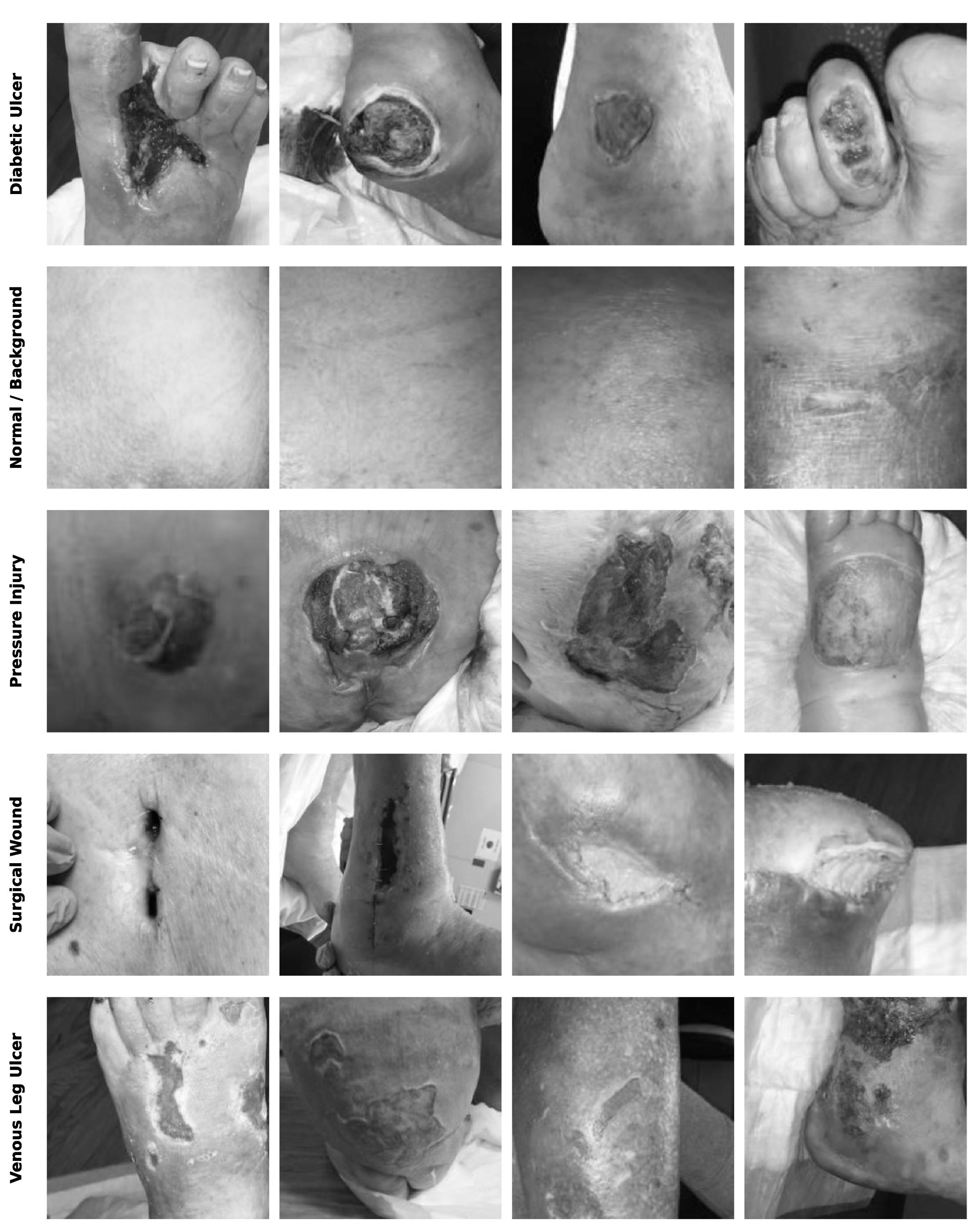
Figure 2.
Statistical variability of macro-F1 scores across the five patient-level cross-validation folds for each backbone architecture. Swin-Tiny and ConvNeXt-Tiny show the tightest inter-fold spread, while ResNet-50 and EfficientNet-B0 are more variable.
Figure 2.
Statistical variability of macro-F1 scores across the five patient-level cross-validation folds for each backbone architecture. Swin-Tiny and ConvNeXt-Tiny show the tightest inter-fold spread, while ResNet-50 and EfficientNet-B0 are more variable.
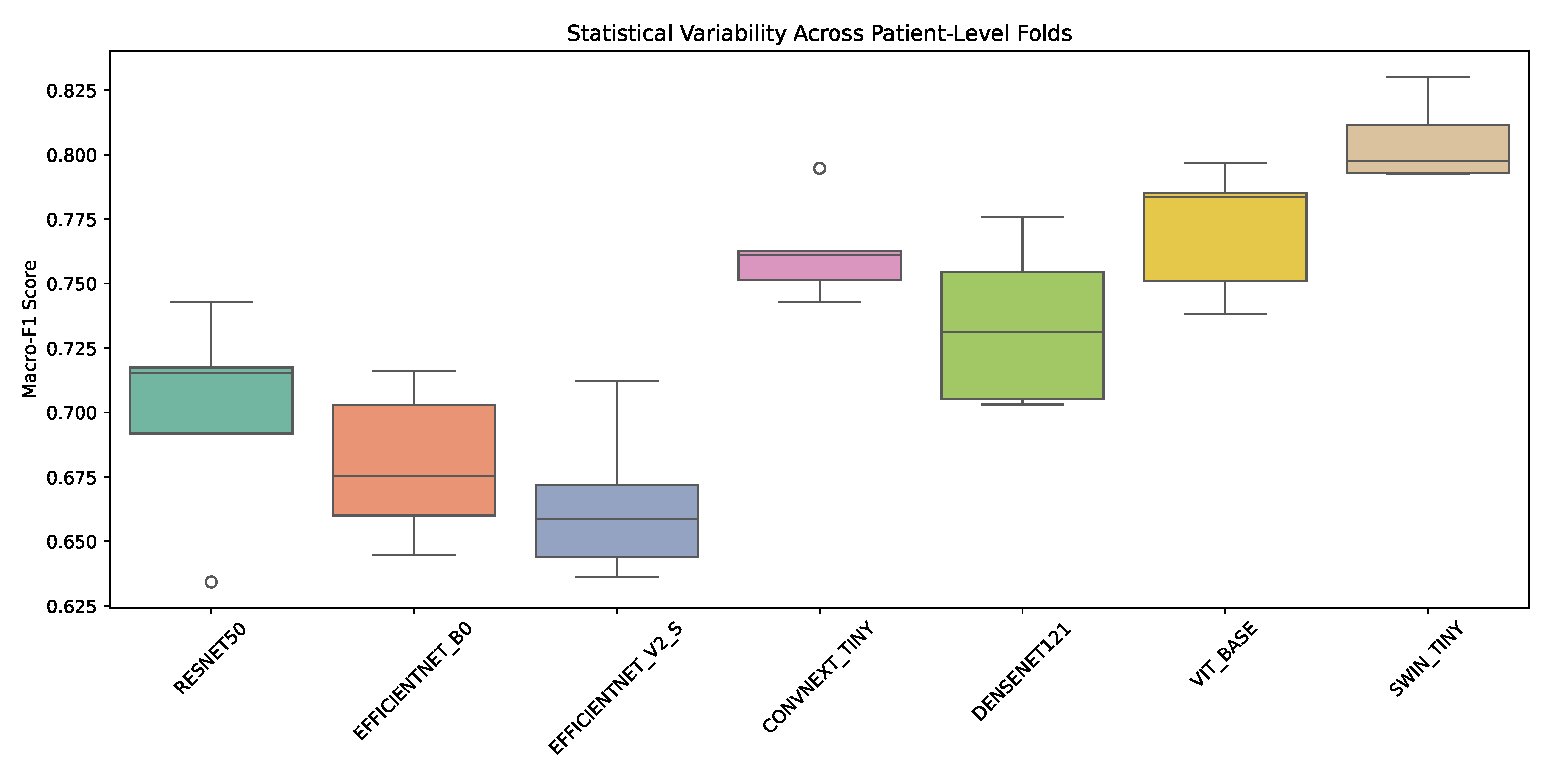
Figure 3.
Per-class receiver operating characteristic (ROC) curves for the top-performing model (Swin-Tiny) on the held-out test set.
Figure 3.
Per-class receiver operating characteristic (ROC) curves for the top-performing model (Swin-Tiny) on the held-out test set.
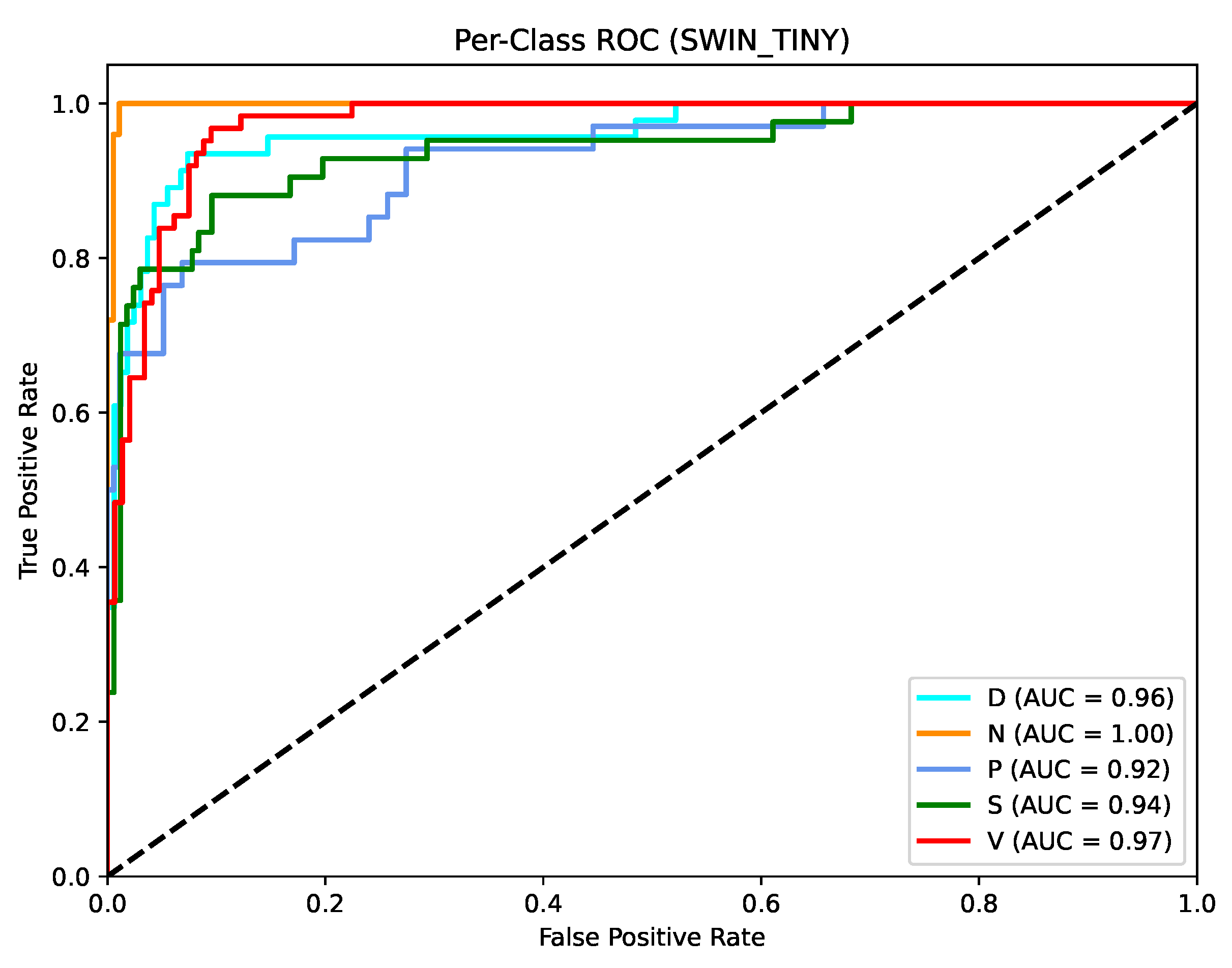
Figure 4.
Normalized confusion matrices for all seven backbones on the held-out test set. Rows represent true class and columns represent predicted class; cell values are row-normalized percentages.
Figure 4.
Normalized confusion matrices for all seven backbones on the held-out test set. Rows represent true class and columns represent predicted class; cell values are row-normalized percentages.
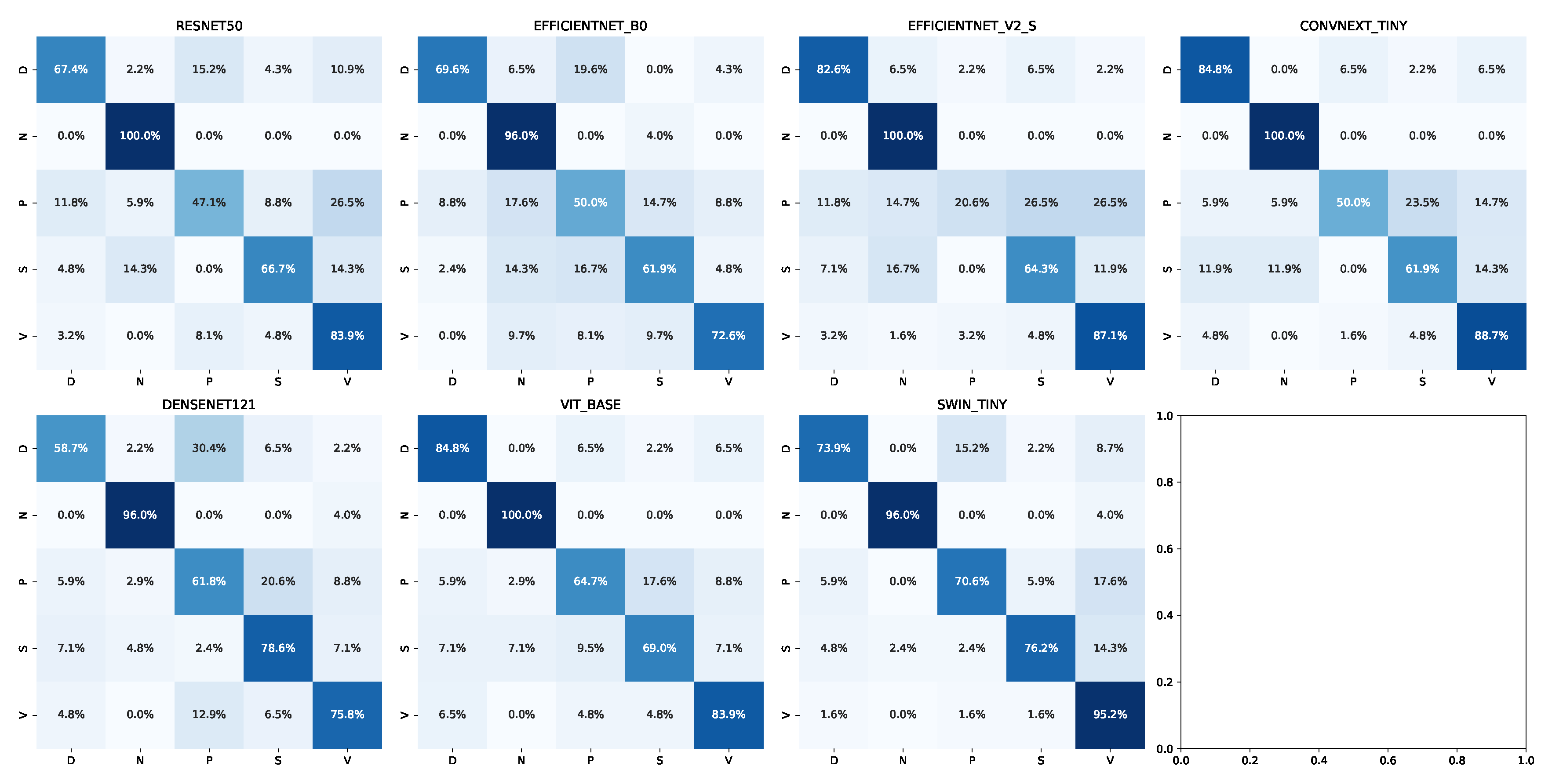
Figure 5.
Top: latent concept (prototype) activation strengths for a sample of held-out test images, annotated with true (T) and predicted (P) class. Bottom: learned weights mapping each of the 32 latent concepts to each of the five etiology classes, for the top-performing model (Swin-Tiny).
Figure 5.
Top: latent concept (prototype) activation strengths for a sample of held-out test images, annotated with true (T) and predicted (P) class. Bottom: learned weights mapping each of the 32 latent concepts to each of the five etiology classes, for the top-performing model (Swin-Tiny).
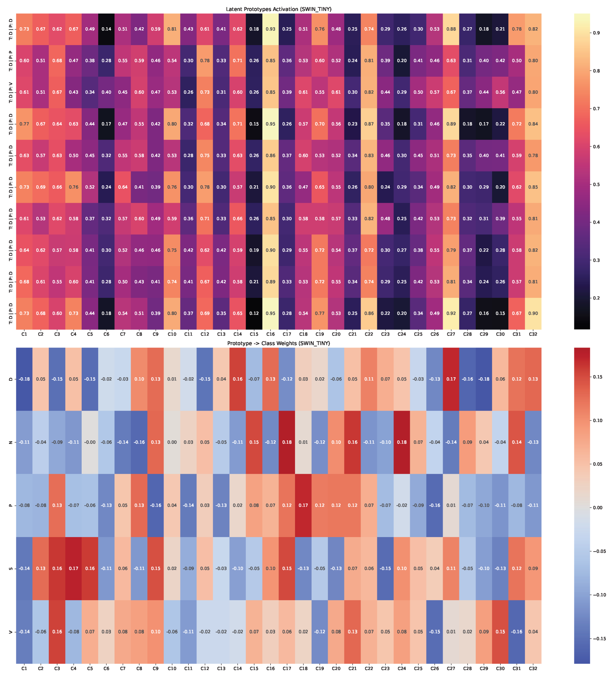

Table 1.
Implementation and Reproducibility Details for the GNN-CBM Framework.
| Parameter / Configuration | Value / Setting |
|---|---|
| Hardware | Single NVIDIA Tesla T4 GPU (16GB VRAM) |
| Software Framework | PyTorch, PyTorch Geometric 2.8.0, Python 3.12 |
| Random Seed | 42 (applied universally to numpy, random, torch) |
| Optimizer | Adam, with differential learning rates for backbone vs. head |
| Learning Rate (Backbone) | |
| Learning Rate (Head/GNN/CBM) | |
| Dropout Rate (Fusion Layer) | 0.3 |
| Batch Size | 32 |
| Epochs | 25 (maximum) |
| Early Stopping | Patience = 5 epochs, min. improvement |
| Concept Bottleneck Width | latent concepts, with residual bypass |
| Anatomical Graph | nodes (20×20 grid), 4-connected, mean degree 3.80 |
| Spatial Penalty Weight | (full model); (ablation) |
| Data Augmentation | Resize , horizontal flip, rotation (), color jitter |
Table 2.
Per-fold test performance for all seven backbones under the full GNN-CBM configuration (), 5-fold stratified group cross-validation.
Table 2.
Per-fold test performance for all seven backbones under the full GNN-CBM configuration (), 5-fold stratified group cross-validation.
| Backbone | Fold | Val. Loss | Test Accuracy | Test Macro-F1 |
|---|---|---|---|---|
| ResNet-50 | 1 | 1.0268 | 0.727 | 0.715 |
| 2 | 1.0179 | 0.656 | 0.634 | |
| 3 | 0.9450 | 0.727 | 0.717 | |
| 4 | 1.2137 | 0.708 | 0.692 | |
| 5 | 1.0106 | 0.751 | 0.743 | |
| EfficientNet-B0 | 1 | 1.0286 | 0.641 | 0.645 |
| 2 | 0.9883 | 0.684 | 0.660 | |
| 3 | 1.0038 | 0.727 | 0.716 | |
| 4 | 1.1227 | 0.713 | 0.703 | |
| 5 | 0.9756 | 0.689 | 0.676 | |
| EfficientNetV2-S | 1 | 0.9660 | 0.722 | 0.672 |
| 2 | 1.0794 | 0.675 | 0.636 | |
| 3 | 1.0277 | 0.679 | 0.659 | |
| 4 | 1.2581 | 0.737 | 0.712 | |
| 5 | 0.9806 | 0.689 | 0.644 | |
| ConvNeXt-Tiny | 1 | 0.8482 | 0.770 | 0.763 |
| 2 | 0.8851 | 0.756 | 0.743 | |
| 3 | 0.8227 | 0.775 | 0.761 | |
| 4 | 0.9516 | 0.799 | 0.795 | |
| 5 | 0.8681 | 0.761 | 0.751 | |
| DenseNet-121 | 1 | 0.8348 | 0.727 | 0.731 |
| 2 | 1.1323 | 0.727 | 0.703 | |
| 3 | 0.9085 | 0.780 | 0.776 | |
| 4 | 1.2327 | 0.718 | 0.705 | |
| 5 | 0.9235 | 0.770 | 0.755 | |
| ViT-Base | 1 | 0.8209 | 0.799 | 0.797 |
| 2 | 0.9069 | 0.794 | 0.785 | |
| 3 | 0.8901 | 0.766 | 0.751 | |
| 4 | 1.0216 | 0.789 | 0.784 | |
| 5 | 0.9686 | 0.742 | 0.738 | |
| Swin-Tiny | 1 | 0.8643 | 0.799 | 0.798 |
| 2 | 0.8900 | 0.799 | 0.793 | |
| 3 | 0.8737 | 0.818 | 0.811 | |
| 4 | 0.9856 | 0.799 | 0.793 | |
| 5 | 0.8582 | 0.828 | 0.830 |
Table 3.
Aggregated clinical performance, calibration, and efficiency metrics (mean ± SD [95% CI] where available) across 5-fold patient-grouped cross-validation. Params and GFLOPs reflect published architecture specifications; ECE and inference time are averaged over cross-validation folds.
Table 3.
Aggregated clinical performance, calibration, and efficiency metrics (mean ± SD [95% CI] where available) across 5-fold patient-grouped cross-validation. Params and GFLOPs reflect published architecture specifications; ECE and inference time are averaged over cross-validation folds.
| Backbone | Accuracy | F1 (macro) | AUC | ECE | Inference (ms) | Params (M) | GFLOPs |
|---|---|---|---|---|---|---|---|
| Swin-Tiny | 0.954 | 0.056 | 5.15 | 28.3 | 4.5 | ||
| ConvNeXt-Tiny | 0.934 | 0.074 | 8.28 | 28.6 | 4.5 | ||
| ViT-Base | 0.951 | 0.064 | 13.23 | 86.6 | 17.6 | ||
| DenseNet-121 | 0.942 | 0.053 | 3.25 | 8.0 | 2.9 | ||
| ResNet-50 | 0.926 | 0.057 | 3.30 | 25.6 | 4.1 | ||
| EfficientNetV2-S | 0.921 | 0.082 | 3.37 | 21.5 | 2.9 | ||
| EfficientNet-B0 | 0.919 | 0.084 | 1.40 | 5.3 | 0.4 |
Table 4.
Per-class precision, recall, and F1 for the top-performing model (Swin-Tiny) on the held-out test set.
Table 4.
Per-class precision, recall, and F1 for the top-performing model (Swin-Tiny) on the held-out test set.
| Class | Precision | Recall | F1 |
|---|---|---|---|
| Diabetic (D) | 0.872 | 0.739 | 0.800 |
| Normal/Background (N) | 0.960 | 0.960 | 0.960 |
| Pressure (P) | 0.727 | 0.706 | 0.716 |
| Surgical (S) | 0.889 | 0.762 | 0.821 |
| Venous (V) | 0.776 | 0.952 | 0.855 |
Table 5.
Pairwise McNemar’s test results (continuity-corrected) comparing Swin-Tiny against each remaining backbone. Significance is denoted for (Bonferroni-corrected across six comparisons).
Table 5.
Pairwise McNemar’s test results (continuity-corrected) comparing Swin-Tiny against each remaining backbone. Significance is denoted for (Bonferroni-corrected across six comparisons).
| Comparison (Swin-Tiny vs.) | Discordant Pairs | p-value | Conclusion | |
|---|---|---|---|---|
| EfficientNet-B0 | 51 | 15.9265 | Significant | |
| ResNet-50 | 45 | 9.3389 | 0.00224 | Significant |
| DenseNet-121 | 47 | 8.9415 | 0.00279 | Significant |
| EfficientNetV2-S | 52 | 8.8894 | 0.00287 | Significant |
| ConvNeXt-Tiny | 29 | 3.8017 | 0.05120 | Not significant |
| ViT-Base | 28 | 1.0804 | 0.29862 | Not significant |
Table 6.
Ablation of the Domain-Constrained Spatial Penalty Loss on the top-performing backbone (Swin-Tiny).
Table 6.
Ablation of the Domain-Constrained Spatial Penalty Loss on the top-performing backbone (Swin-Tiny).
| Configuration | Test Macro-F1 | |
|---|---|---|
| Full GNN-CBM model | 0.5 | 0.8051 |
| Ablated (no spatial penalty) | 0.0 | 0.7918 |
Disclaimer/Publisher’s Note: The statements, opinions and data contained in all publications are solely those of the individual author(s) and contributor(s) and not of MDPI and/or the editor(s). MDPI and/or the editor(s) disclaim responsibility for any injury to people or property resulting from any ideas, methods, instructions or products referred to in the content. |
© 2026 by the authors. Licensee MDPI, Basel, Switzerland. This article is an open access article distributed under the terms and conditions of the Creative Commons Attribution (CC BY) license (http://creativecommons.org/licenses/by/4.0/).
Copyright: This open access article is published under a Creative Commons CC BY 4.0 license, which permit the free download, distribution, and reuse, provided that the author and preprint are cited in any reuse.