

Submitted:
02 August 2026
Posted:
04 August 2026
You are already at the latest version
Abstract
This study establishes a systematic geometric characterization of modern Iran's boundaries and associated coastlines within the West Asian continental domain. It provides a reproducible framework for quantifying the scale-dependent complexity of the region's political and maritime frontiers using adaptive-scale methods. For Iran's mainland borders, the analysis yields a box-counting dimension of 1.0714 and a divider dimension of 1.0744. The adjoining regional seashores exhibit higher irregularity; the Caspian Sea coastlines produce fractal dimensions of 1.1120 and 1.1577, while the Persian Gulf's fractal dimensions reach 1.1587 and 1.1742, respectively. Interestingly, all three geographical land and maritime objects occupy broadly intermediate positions within their respective distributions: Iran ranks centrally among its 13 West Asian neighbors, while both regional seas occupy a middle-ground position relative to eighteen published global coastline studies. These findings reveal a hierarchy of boundary intricacy, where marine coastlines consistently demonstrate greater spatial occupancy than terrestrial frontiers. By integrating dual-method estimations with automated scaling, this research offers a substantiated geometric perspective on the Iranian Plateau's position within the broader global cartographic context.
Keywords:
fractal dimension
; borders
; coastlines
; Iran
; West Asia
; Persian Gulf
; Caspian Sea
MSC: Primary 28A80; Secondary 91D20, 65D18
“This is the kingdom which I hold, from the Sacae beyond Sogdia to Kush, and from Sind to Lydia—this is what Ahuramazda, the greatest of gods, bestowed upon me.”— DPh Foundation Inscription, Persepolis, Fars Province, Iran, King of Kings of the Achaemenid Persian Empire, Darius the Great (c. 550–486 B.C.E) [1]
1. Introduction
1.1. Fractal Geometry of Geographic Boundaries
Fractal Foundations.
Irregular natural curves, including coastlines, rivers, and terrestrial boundaries, commonly reveal additional geometric detail as the observation scale becomes finer. Richardson demonstrated empirically that the measured lengths of geographical curves vary systematically with the size of the measuring unit [2]. Mandelbrot subsequently interpreted this scale dependence through statistical self-similarity and fractional dimension, establishing the coastline problem as a foundational application of fractal geometry [3]. For a planar geographical curve, an estimated dimension near indicates comparatively smooth geometry, whereas progressively larger values toward indicate increasing irregularity and spatial occupancy.
Measurement Evolution.
Early geographical analyses primarily used the divider method, in which a fixed-length chord is stepped along a curve and the resulting path length is examined across successive measurement scales. Later work introduced box-counting and related computational procedures that quantify the number of grid cells intersected by a boundary, thereby facilitating implementation within digital cartography and geographic-information systems [4,5]. Contemporary studies generally estimate the scaling exponent through log–log regression and increasingly examine finite scaling windows rather than assuming uniform fractal behavior across every available scale [6,7,8,9]. Consequently, a reported fractal dimension should be interpreted together with the source geometry, spatial resolution, estimation method, and retained scale interval.
Political Boundaries.
Compared with coastlines, the peer-reviewed literature directly addressing national political boundaries remains limited. Longley and Batty provided an early systematic treatment of the fractal measurement of geographical boundaries, while Alesina et al. used border fractal dimension as a measure of political-boundary straightness across 144 non-island countries [5,10]. More recent single-country investigations estimated both the border and coastline dimensions of India and the box dimension of the complete boundary of Saudi Arabia [6,7]. Thus, the available literature establishes the applicability of fractal measurement to national boundaries, but provides only a restricted empirical basis for regional comparisons and does not include modern Iran.
Coastline Literature.
The peer-reviewed coastline literature is broader and encompasses complete national coastlines, mainland coastal curves, islands, bays, and subregional shoreline sections. Foundational estimates were reported for the western coast of Britain and the coastline of South Africa, while later national-scale studies examined Australia and India [3,7,8]. Research on China has addressed its overall and mainland coastlines, the Shandong–Tianjin coastal region, and the coastline of Taiwan [11,12,13,14]. Additional studies have examined the Irish coast, the southern Norwegian coast, Cres Island, Negros Island, and Greenland [15,16,17,18,19]. Regional and local analyses have further considered the Gulf of California and Delaware Bay, illustrating the diversity of geographical objects and measurement conventions represented in the literature [4,20].
Nonrefereed Sources.
Fractal-dimension estimates for coastlines also appear in online datasets, educational resources, and individual research webpages. The Wolfram Data Repository provides automatically generated coastline estimates for 249 countries, dependencies, and territories, while the Fractal Foundation presents an instructional illustration of ruler-based coastline measurement [21,22]. Pietronero additionally reports local box-counting estimates for world coastlines derived from the GSHHS database [23]. Although these resources are useful for visualization, computational exploration, and preliminary context, they do not constitute peer-reviewed geographical studies of explicitly defined national or regional boundary objects.
Literature Convention.
The present study therefore distinguishes peer-reviewed geographical investigations from nonrefereed online estimates. Peer-reviewed studies are used to establish the scientific context and to support the comparative border and coastline analyses, whereas nonrefereed resources are cited only to describe the wider availability of numerical estimates. This restriction reduces the influence of undocumented differences in geographical definition, data resolution, preprocessing, scale selection, and computational implementation. Accordingly, the formal comparisons developed in this study are anchored to the peer-reviewed literature and to estimates generated under the reproducible framework described in Section 2.
1.2. Geographic Setting of Iran
Iran occupies a geographically and historically distinctive position on the Iranian Plateau. Its present territory constitutes both the principal spatial core of a long-standing civilization and a central West Asian state connecting several major continental and maritime regions. This geographical setting provides the broader context for examining the complexity of its modern borders and adjoining coastlines.
Global Position.
In a broad civilizational chronology extending from approximately 3200 B.C.E. to the present, Iran belongs among the oldest enduring centres of human settlement, state formation, and cultural development, alongside the ancient civilizations of Mesopotamia, Egypt, India, China, and Greece [24,25]. Its territory later formed the political and geographical core of the Achaemenid Persian Empire (c. 550–330 B.C.E.), frequently characterized as the first world empire and, at its greatest extent, the largest political formation then established [26]. Extending across parts of Asia, Europe, and Africa, this empire connected the Iranian Plateau with Central Asia, the Indus Valley, Anatolia, the eastern Mediterranean, Mesopotamia, and Egypt.
Regional Position.
Within West Asia, Iran lies between Anatolia and Mesopotamia to the west, the Caucasus and Caspian region to the north, Central and South Asia to the east, and the Arabian Peninsula to the south [25,27]. The country is bordered by the Caspian Sea along its northern margin and by the Persian Gulf and Gulf of Oman along its southern margin, giving it direct geographical access to both enclosed and open marine systems. Its position at the convergence of major mountain chains, plateaus, deserts, terrestrial frontiers, and contrasting coastlines produces substantial variation in boundary configuration and provides a natural regional framework for comparison with the surrounding West Asian countries.
1.3. Study Motivation
Research Context.
Fractal geometry has been applied to a wide range of natural, cultural, and constructed forms associated with Iran. Nevertheless, the existence of an Iran-related fractal literature should not be interpreted as evidence that the country’s political boundaries or complete adjoining coastlines have already been examined. The available studies fall principally into non-geographical applications, geographically related analyses of interior landforms or localized coastal features, and nonrefereed online estimates whose scope and evidential status differ from those of the present study.
Non-Geographical Studies.
A substantial part of the Iran-related literature concerns architecture, landscape design, and the built environment. Previous investigations have examined fractal patterns in Iranian gardens, architectural motifs, traditional urban and architectural organization, the stepped settlement of Masouleh, and the geometry of bazaars and timchehs [28,29,30,31,32]. These studies demonstrate the broad relevance of self-similarity, repetition, scaling, and hierarchical organization within Iranian cultural forms. However, they are principally qualitative, architectural, or urban-morphological investigations and do not estimate the fractal dimensions of Iran’s complete exterior political boundary, its mainland coastline segments, or the complete coastlines of the Persian Gulf and Caspian Sea.
Geographical Studies.
The geographically oriented literature is more directly relevant but remains limited in spatial scope and geographical object. Saberi et al. examined the box-counting dimensions and morphometric characteristics of selected Iranian landforms, whereas Karam et al. investigated the multiscale and multifractal properties of Iran’s topographic surface [33,34]. These analyses characterize interior terrain, elevation profiles, and three-dimensional landscape roughness rather than the two-dimensional exterior curve of the country. Nazari Sarem et al. estimated the box-counting dimensions of selected estuaries and river meanders along the northern Persian Gulf, including Khor Musa, Khor Abd Allah, the Arvand River, and the Dalaki River [35]. Although geographically important, this work concerns localized coastal and fluvial features rather than Iran’s complete coastline or the complete regional coastline of the Persian Gulf.
Nonrefereed Sources.
Several online resources also report or illustrate coastline fractal dimensions. The Wolfram Data Repository provides automatically generated estimates for 249 countries, dependencies, and territories, while the Fractal Foundation presents an educational explanation of coastline measurement and Pietronero reports local box-counting results for world coastlines derived from the GSHHS database [21,22,23]. These resources are useful for computation, visualization, and preliminary comparison, but they are not peer-reviewed geographical studies specifically designed to evaluate Iran’s borders or adjoining regional seas. Consequently, they cannot substitute for a documented analysis based on explicitly defined geographical objects, reproducible preprocessing, scale selection, regression diagnostics, and statistical comparison.
Literature Gap.
Within the peer-reviewed literature reviewed for this study, no investigation was identified that estimates the fractal dimensions of modern Iran’s complete exterior boundary. Similarly, no peer-reviewed study was found that jointly examines Iran’s principal land-border sections, mainland coastline segments, and selected island coastlines, or that provides paired box-counting and divider estimates for the complete regional coastlines of the Persian Gulf and Caspian Sea. The geographically nearest national-scale studies are the box-dimension analysis of the border of Saudi Arabia and the fractal analysis of India [6,7]; however, neither addresses Iran or provides the integrated regional and component-level framework required here.
Regional Relevance.
This absence is notable because Iran occupies a central position within West Asia, adjoining the Caucasus, Central Asia, South Asia, Mesopotamia, the Arabian Peninsula, the Caspian Sea, the Persian Gulf, and the Gulf of Oman. Its exterior boundary therefore combines terrestrial frontiers and contrasting marine coastlines within a geographically and geopolitically important regional system. A systematic analysis of these curves can clarify whether Iran exhibits unusually low, intermediate, or high boundary complexity relative to surrounding countries, while also determining how complexity varies among its western, eastern, northern, and southern components.
Study Contribution.
The present study addresses these gaps through a unified and reproducible framework that applies adaptive-scale box-counting and divider methods to modern Iran, 13 regional comparison countries, the Persian Gulf and Caspian Sea coastlines, Iran’s principal mainland boundary components, and selected island coastlines. By combining explicit geographical definitions, automated scaling-window selection, regression diagnostics, and formal statistical comparisons, the analysis is intended to provide both the first systematic geometric characterization of these Iranian-associated boundaries and a transferable foundation for broader comparative studies of political borders and coastlines.
1.4. Study Outline
This study provides a reproducible, adaptive, dual-method framework for quantifying the scale-dependent geometric complexity of modern Iran’s boundaries and adjoining regional coastlines, and shows that Iran occupies a broadly intermediate position within the West Asian boundary-complexity distribution while exhibiting systematic internal variation among its land-border and coastline components. The remainder of the paper is organized as follows. Section 2 presents the methodological framework, including the study region and geospatial data (Section 2.1), boundary extraction and preprocessing procedures (Section 2.2), object-specific adaptive scale selection (Section 2.3), box-counting and divider fractal-dimension estimation (Section 2.4), the complete stepwise computational workflow (Section 2.5), and the statistical analyses used for benchmark, paired-method, and regional comparisons (Section 2.6). Section 3 reports the empirical results. Section 3.1 examines overall-border complexity across West Asia, Iran’s national and regional land-border estimates, and Iran’s position within the regional fractal-dimension distribution. Section 3.2 evaluates coastline complexity at two geographical levels, first for the complete Persian Gulf and Caspian Sea coastlines and then for Iran’s mainland coastline segments and selected islands. Finally, Section 4 interprets the principal geographical findings (Section 4.1), identifies the methodological contributions of the adaptive computational framework (Section 4.2), and discusses the principal limitations and directions for future research (Section 4.3). The paper concludes by summarizing the broader implications of the findings for comparative analysis of political boundaries, regional seas, and evolving coastlines.
2. Methods
2.1. Study Region and Geospatial Data
The study region comprised modern Iran and 13 neighboring or nearby comparison countries forming a contiguous West Asian geographical domain. This regional frame extends from Anatolia and the South Caucasus through Central and South Asia to the Arabian Peninsula, thereby representing substantial variation in national size, physiography, and boundary configuration. Administrative-level-0 boundary geometries were obtained from the GADM database, Version 4.1 [36].
In this study, the term Modern Iran refers operationally to Iran in its post-1975 state-boundary configuration, following the formal redemarcation of the Iran–Iraq land frontier and delimitation of their river frontier under the 1975 bilateral settlement [37]. The map also emphasizes Iran’s central geographical position between the Caspian Sea, Persian Gulf, and Gulf of Oman and at the convergence of the Caucasian, Central Asian, Arabian Peninsula, and South Asian regions, as shown in Figure 1.
2.2. Boundary Extraction and Preprocessing
Data Source.
Administrative boundary geometries were obtained from the 2022 Global Administrative Areas database, Version 4.1 (GADM 4.1), at administrative level 0 [36]. All geometries were validated before analysis and transformed from longitude–latitude coordinates on the WGS84 datum to metric projected coordinate systems. Vector-topology operations, boundary extraction, coordinate transformation, and raster–vector intersection were implemented in R using the sf and terra packages [39,40]. No geometric smoothing or simplification was applied before fractal-dimension estimation.
National Boundaries.
For Iran and each of the 13 regional comparison countries, the level-0 multipolygon was decomposed into its polygonal components, and the component with the greatest projected area was retained as the main landmass. Interior polygon rings, representing lakes and other enclosed water bodies, were removed, after which the exterior ring of the retained polygon was extracted as a line geometry. Consequently, the analyzed curve contained the complete exterior boundary of the main landmass, including terrestrial frontiers and mainland coastlines, while smaller offshore islands and other disconnected components were excluded. This mainland-only convention is consistent with the geographical object analyzed in previous national-border box-dimension studies [6]. Each national boundary was projected to a country-centred azimuthal equidistant coordinate reference system, with the projection centre defined by the midpoint of its geographic bounding box.
Regional Coastlines.
The Caspian Sea and Persian Gulf objects used for the international coastline comparison were constructed as regional mainland coastlines rather than as the coastline of a single country. For the Caspian Sea, the level-0 geometries of Iran, Turkmenistan, Kazakhstan, Russia, and Azerbaijan were projected to a local Lambert azimuthal equal-area coordinate system, dissolved, and reduced to the largest connected regional land polygon. Because the Caspian Sea is landlocked, its mainland shoreline was represented by an interior ring of this dissolved polygon. The target ring was identified by the seed point . If direct containment failed because of numerical topology, the interior ring whose centroid was nearest to the seed was selected. Offshore island coastlines were not retained.
For the Persian Gulf, the level-0 geometries of Iran, Iraq, Kuwait, Saudi Arabia, Qatar, the United Arab Emirates, and Oman were projected, dissolved, and reduced to the largest connected regional land polygon. The exterior ring was divided at the GADM vertices nearest Cape al-Kuh, Iran, and Ras Limah, Oman, which define the hydrographic limit between the Persian Gulf and Gulf of Oman [41]. Of the two possible arcs joining these endpoints, the Persian Gulf arc was selected according to the proportion of its vertices contained within the prespecified regional envelope and, where necessary, its proximity to the guide point . The endpoint-to-endpoint closure line was used only to define the hydrographic limit and was not included in the measured coastline; offshore islands were likewise excluded. The extracted regional coastlines were subsequently transformed to coastline-centred azimuthal equidistant projections for metric measurement.
Iranian Boundary Components.
For the national component analysis, the exterior ring of mainland Iran was partitioned into five mutually exhaustive segments: the Western and North-Western Border Section (WNBS), Caspian Coastline Segment (CCS), Eastern and North-Eastern Border Section (ENBS), Gulf of Oman Coastline Segment (GOCS), and Persian Gulf Coastline Segment (PGCS). Five geographical transition seeds identified the Iran–Iraq/Persian Gulf junction, Astara, the eastern Caspian/Turkmenistan junction, the Pakistan/Gulf of Oman junction, and Cape al-Kuh. Each seed was snapped to the nearest existing GADM exterior-ring vertex, and a component-specific guide point was used to select the intended arc between successive anchors. Thus, the procedure partitioned the original GADM ring without redrawing or simplifying it. As a numerical validation, the sum of the five extracted segment lengths was required to reproduce the mainland perimeter with relative error below .
The ten island coastlines were extracted from the individual GADM polygon components corresponding to Lavan, Hendurabi, Kish, Farur, Sirri, Abu Musa, Qeshm, Hengam, Larak, and Hormuz. Each island was identified by a point located within its polygon, and the procedure required exactly one non-mainland polygon to contain each point; otherwise, execution was terminated. Only the exterior ring of each selected island polygon was retained. All 15 Iranian components (2 land-border segments, 3 coastline segments and 10 islands) were transformed to an Iran-centred Lambert conformal conic projection on WGS84, with standard parallels at and N, latitude of origin N, and central meridian E.
2.3. Adaptive Scale Selection
Scale Calibration.
A common fixed scale range was not imposed because the analyzed objects differed markedly in geographical extent, ranging from large national boundaries to small island coastlines. Candidate scales were therefore calibrated separately for each geographical object. Let W and H denote the width and height, in kilometres, of the projected bounding box; define
and let denote the 25th percentile of the positive native inter-vertex segment lengths s. The finest candidate scale combined a hard resolution floor, a native-vertex-spacing guard, and a memory guard limiting the corresponding counting grid to approximately cells.
Countries and Regional Coastlines.
For the 14 national boundaries and the two regional coastlines, the candidate scale range was bounded by
and
where all scale quantities are expressed in kilometres. Hence, the national-boundary and regional-coastline scripts used object-specific candidate ranges within the explicit hard limits –200 km. The upper bound maintained approximately eight boxes across the shorter side of the geographical object while preventing excessively coarse grids. The lower bound prevented unsupported sub-100-m measurement and excessive raster allocation.
Iranian Components and Islands.
The 15 Iranian components required a finer lower bound and a coarse-scale rule that also accommodated long and narrow boundary segments. Their candidate range was defined by
and
Thus, the Iranian component script used object-specific candidate ranges within the explicit hard limits –200 km, retaining scales as fine as 50 m when supported by the source geometry and memory constraint. If the initial upper bound was not greater than the lower bound, it was expanded, where possible, toward km. This distinction between the –200 km country/regional setting and the –200 km component/island setting was introduced to retain useful small-island detail without imposing the same fine-scale requirement on much larger country boundaries.
Candidate Sequence.
Within the applicable object-specific bounds, candidate scales were generated in logarithmic progression:
These candidate ranges should be distinguished from the final selected scaling windows. The selected windows were contiguous subsets of the candidate scales and are reported with the corresponding estimates in Table 1, Table 3, Table 5, and Table 6.
For divider measurement, each line was densified before stepping so that the maximum interpolated segment length satisfied
where km for the national boundaries and regional coastlines and km for the Iranian components. Densification did not alter the underlying geographical path; it inserted intermediate vertices to reduce overshoot during the chord-based divider traversal.
2.4. Fractal-Dimension Estimation
Dimension Selection.
Fractal geometry includes several dimension concepts for characterizing the scale-dependent complexity of an object. These include the Hausdorff, box-counting or Minkowski–Bouligand, divider, packing, Assouad, Higuchi, Lyapunov, and Rényi generalized dimensions, the latter encompassing the capacity, information, and correlation dimensions as principal cases [42,43]. The present study focuses on the box-counting and divider dimensions because they are widely used for the analysis of geographical boundaries and coastlines and provide complementary measures of spatial occupancy and scale-dependent path length. Their joint application also permits direct evaluation of cross-method agreement under a common adaptive-scale framework.
Scaling Laws.
Geometric complexity was estimated using the box-counting and divider (Richardson) dimensions, which describe complementary forms of scale-dependent boundary measurement [2,3]. Let denote the number of square boxes of side length required to cover a boundary. Under box-counting scaling,
so that
Accordingly, the box-counting dimension was obtained as the negative ordinary least-squares slope:
For the divider method, let denote the effective number of divider steps of length , and let
denote the measured boundary length. Richardson scaling gives
which yields
Box-Counting Procedure.
At each candidate scale, a regular square grid was superimposed on the projected boundary and all cells intersected by the line were counted. To reduce dependence on grid placement, four origins were evaluated, corresponding to offsets of 0 and along each coordinate axis. If denotes the count under translation t, the retained count was
The minimum translated count approximates the minimal cover underlying the box-counting definition. Candidate scales yielding fewer than eight intersecting boxes were excluded before regression, thereby avoiding unstable fits dominated by very coarse grids [9].
Divider Procedure.
For each densified line, the divider traversal began at the first vertex and advanced to the first subsequent vertex whose chord distance from the current anchor was at least . This vertex became the next anchor, and the procedure continued until the end of the line. To prevent the final incomplete segment from being discarded, the residual terminal polyline length, , was included as a fractional step:
For geographical objects containing more than one line, the effective counts were summed over all lines. Scales yielding fewer than eight effective divider steps were excluded. The measured length was then calculated using Equation (11).
Scaling-Window Selection.
Natural boundaries generally exhibit approximate power-law behavior over finite scale intervals rather than over every available scale [3,6]. For each method, ordinary least-squares models were therefore fitted to every contiguous candidate window containing at least six admissible scales. Only windows yielding a planar-curve dimension within were considered theoretically admissible.
Let denote the adjusted coefficient of determination for window w, and let be its maximum over all admissible windows. The near-optimal set was defined as
Among these windows, the window spanning the widest interval in was selected. Ties were resolved by the larger number of retained scales and then by the larger adjusted . This rule prioritized breadth of scaling evidence over negligible improvements in fit. If no admissible window existed, the window whose estimated dimension was closest to the interval was retained only as a flagged diagnostic fallback; the estimated value was not truncated or otherwise forced into the admissible interval.
The primary dimension estimates, unadjusted values, and scale windows reported in the manuscript were obtained from the selected regressions. Full-candidate-range estimates, all examined windows, scale diagnostics, count tables, fitted models, and extracted geometries were archived as reproducibility outputs. Because adjusted contributed to selecting the final window, the reported values quantify linearity within the selected interval and should not be interpreted as independent validation of the estimated dimension. The log–log regressions were supported by the fractaldim package, whereas the planar box counts, divider walks, adaptive scales, and scaling-window search were implemented using purpose-built routines [9,44]. Figure 2 presents the two fractal dimension estimations procedure evaluations for the case of Iran’s mainland borders.
2.5. Overall Stepwise Computational Procedure
The complete computation, from geospatial data acquisition to regional aggregation, proceeded through ten sequential steps applied consistently to each of the 14 countries (and with minor edits for Iranian components).
Step 1: Data acquisition.
The GADM 4.1 administrative-level-0 GeoPackage corresponding to each country’s ISO-3 code was downloaded from the GADM repository, and the downloaded file was checked for availability and integrity.
Step 2: Geometry validation and component selection.
The level-0 layer was imported, invalid geometries were repaired, and each country multipolygon was decomposed into its constituent polygonal components; the component with the greatest projected area was retained as the principal mainland.
Step 3: Boundary extraction.
Interior lacustrine rings were removed, the retained land geometry was unified, and its exterior boundary was extracted as line geometry and archived for reproducibility.
Step 4: Local metric projection.
A country-centred azimuthal equidistant coordinate reference system on the WGS84 datum was constructed at the midpoint of the geographical bounding box, and the extracted boundary was transformed to metric coordinates.
Step 5: Adaptive scale calibration.
The projected bounding-box dimensions and native inter-vertex segment-length distribution were calculated; the country-specific coarsest and finest candidate scales, and , were then determined from Equations (2) and (3), and logarithmically spaced candidate scales were generated according to Equation (6).
Step 6: Translated-grid box counting.
At every candidate scale, square grids were constructed at four translated origins, the boundary-intersecting cells were counted, and the minimum translated count was retained according to Equation (15); scales containing fewer than eight occupied boxes were excluded.
Step 7: Divider counting.
Step 8: Scaling-window selection.
For each estimation method, ordinary least-squares regressions were fitted to every contiguous window containing at least six admissible scales. Among windows producing dimensions within , the window with the widest logarithmic scale span was selected from those lying within of the maximum adjusted , as formalized in Equation (17); when no admissible window existed, the closest window was retained and explicitly flagged as a diagnostic fallback.
Step 9: Dimension estimation.
Step 10: Archiving and regional aggregation.
For each country, the extracted boundary, count tables, examined scaling windows, scale diagnostics, dimension summaries, regression figures, and serialized computational object were saved; the final estimates were then appended to the regional summary, after which the combined results table, execution log, and pooled scale diagnostics were exported.
2.6. Statistical Analysis
Quantities.
For each collection of fractal-dimension estimates, the median, first and third quartiles, arithmetic mean, minimum, maximum, standard deviation, standard error, interquartile range, relative standard error, and percentage excess above the linear benchmark were reported. Here, and denote the first and third quartiles; denotes the standard deviation; denotes the standard error of the mean; and denotes the interquartile range. The relative standard error was calculated as
where is the sample mean fractal dimension. The percentage excess relative to the benchmark was calculated as
where was taken as the linear benchmark for a geometrically smooth one-dimensional curve.For paired method comparisons, the component-level difference was defined as
In the comparison of Iran with the regional reference distribution, the raw difference was defined as
and the standardized difference was calculated as
Iran’s rank was reported in ascending order among all countries included in the corresponding comparison. The symbol denotes the sample mean in parametric analyses and the Hodges–Lehmann pseudomedian in Wilcoxon analyses. Unless otherwise stated, uncertainty was summarized using 95% confidence intervals. One-sided lower confidence intervals were reported for tests against , whereas two-sided confidence intervals were reported for paired-method comparisons. For single-case comparisons, 95% reference intervals represented the expected range of an individual observation drawn from the regional reference distribution.
Hypothesis Tests.
One-sample t-tests were used to test whether the mean fractal dimension was greater than the linear benchmark,
The corresponding nonparametric analyses were conducted using one-sample Wilcoxon signed-rank tests. Differences between the box-counting and divider estimates were examined using paired t-tests and paired Wilcoxon signed-rank tests under the hypotheses
Exact Wilcoxon procedures were used when no zero differences or tied absolute differences were present.
Missing Data Visualization
In many occasions there are published studies in which instead of reporting pairs of fractal dimension estimations, there is only one fractal-dimension estimation. Here, for visualization, one-metric data are displayed as equality-line projections in the Box.Counting-Divider plane, with dotted guide segments indicating the missing coordinate. This approach is special case of deterministic regression imputation that preserves the published one-dimensional information while visually distinguishing incomplete observations from fully observed bivariate pairs [45,46,47].
Side Considerations
Distributional assumptions were evaluated using the Shapiro–Wilk normality test. Potential outliers were identified using the conventional criterion. When departures from normality or potential outliers were detected, both parametric and nonparametric findings were reported, with the Wilcoxon results serving as a robustness analysis. All tests used a significance level of , and all reported p-values were interpreted according to the prespecified one-sided or two-sided alternative hypothesis.
Iran’s individual fractal-dimension estimate was compared with the 13-country regional reference sample using the two-sided Crawford–Howell modified t-test [48]. This procedure accounts for the additional uncertainty associated with comparing a single observation with a small reference sample. For the box-counting and divider single-case comparisons, Holm-adjusted p-values were additionally examined to control the family-wise error rate [49].
Software.
All fractal dimension computations and statistical analyses were performed in R [50]. Fractal-dimension estimation was supported by the peer-reviewed fractaldim package, Version 0.8-5 [9,44]. Descriptive summaries, Shapiro–Wilk diagnostics, t-tests, Wilcoxon signed-rank tests, confidence-interval calculations, and Holm adjustments were performed using functions from the base stats package together with custom R routines. Custom implementations were also used for the Crawford–Howell modified t-tests and their associated reference intervals.
3. Results
3.1. Overall-Border Complexity
3.1.1. West Asia: Regional Patterns in Fractal Dimensions
Table 1 summarizes the adaptive-scale fractal-dimension estimates for the main-landmass boundaries of Iran and 13 surrounding countries. The results are discussed in three directions as follows:
Fractal Dimensions.
All estimates exceeded the linear benchmark and remained well below the plane-filling benchmark , indicating varying degrees of boundary irregularity over the selected spatial scales. The box-counting estimates ranged from for Oman to for Bahrain, whereas the divider estimates ranged from for Kuwait to for the United Arab Emirates. Most estimates were concentrated between approximately and , suggesting that the boundaries generally possess low-to-moderate fractal complexity, although meaningful differences remain among the countries. The mean estimates obtained from the box-counting and divider methods were and , respectively, demonstrating close overall agreement between the two approaches. Nevertheless, the country-level rankings were not identical. Bahrain had the highest box-counting estimate, whereas the United Arab Emirates had the highest divider estimate. The largest absolute differences between the two methods occurred for Bahrain (), Azerbaijan (), and Armenia (); in contrast, the estimates for Saudi Arabia differed by only . These results indicate that, although the methods are consistent at the regional level, some individual boundaries remain sensitive to the adopted estimation procedure.
Fit Statistics(R-Squared).
The regression fits were uniformly strong. The box-counting coefficients of determination ranged from to , while the corresponding divider values ranged from to . Moreover, the box-counting method produced a higher value for every country. This finding indicates a more nearly linear log–log relationship within the scale windows selected by the box-counting procedure. It should not, however, be interpreted by itself as proof that the box-counting estimates are necessarily more accurate, because evaluates goodness of fit within the selected scaling interval rather than agreement with an independently known dimension. Even the lowest divider value, observed for Kuwait (), represents a comparatively strong linear fit.
Scale Windows.
A systematic difference was also observed in the selected scale windows. For every country, the box-counting window covered a wider range of spatial scales than its divider counterpart. Iran had the widest selected window under both methods, extending from to km for box counting and from to km for the divider method. In contrast, Bahrain had the narrowest box-counting window (– km), while Qatar had the narrowest divider window (– km). Thus, the two methods do not necessarily identify the same spatial scaling regime, and their estimates should be interpreted together with their respective scale windows. Finally, because the calculations exclude smaller offshore islands, the reported dimensions characterize the main landmass of each country rather than its complete territorial boundary.

Table 1.
Fractal dimension estimations of Iran’s main landmass borders and the West Asian neighbors using adaptive methods
Table 1.
Fractal dimension estimations of Iran’s main landmass borders and the West Asian neighbors using adaptive methods
| Country | Fractal Dimension and its Statistics | |||||
|---|---|---|---|---|---|---|
| Box-Counting | Divider | |||||
|
Selected scale window (km) |
Selected scale window (km) |
|||||
| Iran | 1.071385 | 0.999860 | 1.3980–200.0000 | 1.074387 | 0.992007 | 4.4945–83.2994 |
| Türkiye | 1.121568 | 0.999760 | 0.8724–87.1355 | 1.097811 | 0.998747 | 3.3791–13.0833 |
| Armenia | 1.068096 | 0.999374 | 0.2224–33.8644 | 1.104379 | 0.974999 | 1.7612–25.1971 |
| Azerbaijan | 1.070637 | 0.998938 | 0.3432–48.7613 | 1.112712 | 0.992843 | 4.7330–27.2171 |
| Turkmenistan | 1.064653 | 0.999901 | 0.8297–105.9690 | 1.071477 | 0.995071 | 4.5951–45.0281 |
| Afghanistan | 1.079860 | 0.999221 | 0.9373–126.4500 | 1.060715 | 0.990907 | 5.2924–22.3943 |
| Pakistan | 1.083402 | 0.999783 | 1.1572–172.8401 | 1.078196 | 0.998886 | 5.0453–29.5303 |
| Oman | 1.042343 | 0.999922 | 0.7089–102.0399 | 1.050930 | 0.972937 | 5.4859–23.6598 |
| UAE | 1.116819 | 0.999886 | 0.3518–47.7571 | 1.127219 | 0.996752 | 0.8368–20.0755 |
| Saudi Arabia | 1.062830 | 0.999974 | 1.5783–200.0000 | 1.063455 | 0.992237 | 3.7092–27.2369 |
| Qatar | 1.127751 | 0.999543 | 0.1051–11.0774 | 1.114452 | 0.994192 | 0.5439–2.1404 |
| Bahrain | 1.151084 | 0.999737 | 0.1000–4.4079 | 1.105864 | 0.990016 | 0.2437–2.2598 |
| Kuwait | 1.045121 | 0.999879 | 0.1457–21.6151 | 1.036536 | 0.963704 | 1.1415–12.0034 |
| Iraq | 1.042969 | 0.999890 | 0.7537–114.9590 | 1.038794 | 0.994275 | 4.4442–19.4962 |
Notes: Fractal-dimension estimates were based on the main landmass of each country, excluding smaller islands. denotes the estimated fractal dimension and the coefficient of determination. Estimates and are reported to six decimal places; scale windows (km), reported to four decimals, indicate the ranges retained for regression. UAE denotes United Arab Emirates.
Figure 3 compares the box-counting and divider fractal-dimension estimates for the boundaries of Iran and its 13 neighboring or nearby countries. The overall upward distribution of the points indicates a positive relationship between the two methods: countries with relatively low box-counting dimensions generally also have relatively low divider dimensions, whereas countries with more complex boundaries tend to receive higher estimates under both procedures.
Visual Groups.
Four broad visual groupings may be distinguished. Group 1(Oman, Iraq, and Kuwait) occupies the lower-left portion of the diagram; Group 2(Afghanistan, Saudi Arabia, Turkmenistan, Iran, and Pakistan) forms a lower-middle group; Group 3(Armenia and Azerbaijan) is characterized by comparatively high divider dimensions relative to their box-counting estimates; and Group 4(Türkiye, the United Arab Emirates, Qatar, and Bahrain) occupies the region associated with generally higher paired dimensions. These groupings progress broadly from lower to higher boundary complexity, although some overlap is present and they should not be interpreted as the outcome of a formal cluster analysis.
Visual Method Agreement.
The dashed line represents perfect agreement between the two estimation methods. Saudi Arabia lies closest to this line, followed by Iran, Iraq, Pakistan, and Turkmenistan, indicating that the two procedures yield highly similar estimates for these countries. Iran, highlighted by the diamond marker, lies only slightly above the equality line, showing that its divider estimate is marginally greater than its box-counting estimate.
Visual Method Differences.
The largest departures from the equality line are observed for Bahrain, Azerbaijan, and Armenia. Bahrain lies distinctly below the diagonal, indicating that its box-counting estimate is substantially higher than its divider estimate. In contrast, Azerbaijan and Armenia lie above the diagonal and therefore receive higher fractal-dimension estimates under the divider method. Türkiye and Afghanistan also fall noticeably below the reference line.
In overall, Figure 3 demonstrates a general degree of consistency between the two approaches while showing that the estimated complexity of some national boundaries remains sensitive to the estimation method and its associated scale-selection procedure.
Table 1 complements the country-level results and their corresponding visual comparison by summarizing the distributions of the box-counting and divider estimates and by formally examining two questions: whether the border dimensions are greater than the linear benchmark , and whether the two estimation methods produce systematically different results across the 14 countries.
Descriptive Statistics.
The mean box-counting dimension was (), compared with () for the divider method. The corresponding medians were and , respectively. Thus, both the means and medians were closely aligned across the two methods. The box-counting estimates exhibited slightly greater dispersion, with an SD of , an IQR of , and an observed range of –, compared with an SD of , an IQR of , and a range of – for the divider estimates. Nevertheless, the relative standard errors were below for both methods, indicating precise estimation of the corresponding sample means. Moreover, the mean dimensions exceeded the linear benchmark by approximately for box counting and for the divider method, demonstrating nearly identical average departures from .
One-Sample Tests.
Both the parametric and nonparametric analyses provided strong evidence that the border dimensions were greater than . The one-sample t-tests were significant for both the box-counting and divider estimates (), with one-sided confidence intervals of and , respectively. The Wilcoxon tests led to the same conclusion, yielding estimated pseudomedians of and , with lower confidence limits of and , respectively, and in both cases. Since all lower confidence limits were above 1, the results consistently reject the hypothesis that the national boundaries behave as geometrically smooth one-dimensional lines over the selected scale ranges. Instead, they support the presence of measurable boundary irregularity and fractal complexity throughout the studied region.
Paired Tests.
The paired analyses found no evidence of a systematic difference between the two estimation methods. The mean paired difference, defined as the box-counting estimate minus the divider estimate, was only , with a confidence interval of and . Similarly, the Wilcoxon signed-rank test produced an estimated median paired difference of , with a confidence interval of and . Both intervals contained zero, and both point estimates were very close to zero. Therefore, although individual countries may display method-specific deviations, the two procedures yield statistically comparable fractal-dimension estimates at the regional level. This absence of statistical significance should be understood as a lack of evidence for a systematic difference, rather than as formal proof that the methods are exactly equivalent.
Table 2.
Descriptive Statistical Analysis of border fractal dimensions across Iran and neighboring West Asian countries (n = 14)
Table 2.
Descriptive Statistical Analysis of border fractal dimensions across Iran and neighboring West Asian countries (n = 14)
| Statistics | |||
| (a) Descriptive statistics | |||
| Median (Q1, Q3) | 1.0710 (1.0630, 1.1080) | 1.0763 (1.0610, 1.1050) | |
| Mean (Min, Max) | 1.0820 (1.0423, 1.1511) | 1.0812 (1.0365, 1.1272) | |
| SD (SE) | 0.0342 (0.0091) | 0.0294 (0.0079) | |
| IQR (Q3 - Q1) | 0.045 | 0.044 | |
| RSE (%) | 0.84% | 0.73% | |
| (%) | 8.20% | 8.12% | |
| (b) One-sample Tests: . | |||
| t-test | |||
| (95% CI) | 1.0820 (1.0658, ) | 1.0812 (1.0673, ) | |
| Sig. (1-sided) | |||
| Wilcoxon test | |||
| (95% CI) | 1.0796 (1.0629, ) | 1.0819 (1.0672, ) | |
| Sig. (1-sided) | |||
| (c) Paired-sample Tests: . | |||
| t-test | |||
| (95% CI) | 0.0008 (-0.0122, 0.0138) | ||
| Sig. (2-sided) | 0.893 | ||
| Wilcoxon test | |||
| (95% CI) | 0.0016 (-0.0115, 0.0133) | ||
| Sig. (2-sided) | 0.808 | ||
Notes: Statistical quantities and tests are defined in Section 2.5. Panel (b) reports one-sided 95% lower confidence intervals; Panel (c) reports two-sided intervals for box-counting minus divider differences.
3.1.2. Iran’s Overall Border: Fractal-Dimension Estimates
The results obtained specifically for Iran are summarized below in Table 3, with particular attention to the estimated dimensions, the quality of the scaling regressions, and overall and local land borders.
Table 3.
Fractal dimension estimations of overall and local Iran’s borders using adaptive methods
| Country | Fractal Dimension and its Statistics | |||||
|---|---|---|---|---|---|---|
| Box-Counting | Divider | |||||
|
Selected scale window (km) |
Selected scale window (km) |
|||||
| Iran(Overall) | 1.071385 | 0.999860 | 1.3980–200.0000 | 1.074387 | 0.992007 | 4.4945–83.2994 |
| Iran(WNBS)* | 1.055800 | 0.999767 | 0.5520–51.6412 | 1.067295 | 0.985832 | 2.7391–10.4070 |
| Iran(ENBS)* | 1.037482 | 0.999789 | 0.9386–115.8103 | 1.048980 | 0.990162 | 9.0490–49.5106 |
Notes: Fractal-dimension estimates were based on the main landmass of Iran, excluding smaller islands. WNBS: Land borders with Iraq, Türkiye, Armenia, and Azerbaijan. ENBS: Land borders with Turkmenistan, Afghanistan, and Pakistan.
Fractal Dimensions.
Iran’s box-counting and divider dimensions were estimated as follows:
The difference between the two estimates was only , corresponding to less than of their average value. This small discrepancy indicates strong agreement between the two independently applied procedures and suggests that the estimated fractal complexity of Iran’s exterior border is not strongly dependent on the selected measurement method.
Regional Comparison.
Relative to Iran’s overall exterior border, both regional segments produced lower dimension estimates. For WNBS, the box-counting and divider estimates were lower by 0.0156 and 0.0071, respectively, whereas the corresponding reductions for ENBS were 0.0339 and 0.0254. Thus, the complete exterior boundary exhibits slightly greater estimated geometric complexity than either regional segment considered separately.
Local Comparison.
Iran’s Western and North Western Border Section (WNBS) consistently produced higher fractal dimensions than its Eastern and North Eastern Border Section (ENBS), exceeding it by approximately 0.0183 under both estimation methods. This identical difference preserves the regional ordering across methods and indicates modestly greater boundary irregularity along the western–northern segment. Nevertheless, all regional estimates remain relatively close to suggesting that the contrast between the two segments is systematic but not pronounced.
Scaling Behavior.
As illustrated in Figure 4, both methods exhibit an approximately linear log–log scaling relationship within their automatically selected scale windows. The box-counting regression produced an exceptionally high coefficient of determination, , over the comparatively broad scale interval of – km. The divider regression also showed a strong fit, with , although its selected interval was narrower, extending from to km. The excluded divider observations at the smallest and largest candidate scales indicate that the most stable divider scaling behavior occurs over an intermediate spatial range. Thus, while both procedures support a clear scaling structure, the box-counting method identifies a broader and more nearly linear scaling regime for Iran’s border.
Interpretation.
Since both estimated dimensions exceed the smooth-curve benchmark , Iran’s exterior border displays measurable geometric irregularity over the investigated scales rather than behaving as an entirely smooth one-dimensional curve. At the same time, the estimates remain relatively close to 1, indicating low-to-moderate fractal complexity rather than extreme boundary irregularity. Within the present regional sample, Iran occupies an approximately middle position. Under both methods, its estimated border dimension is higher than those of Iraq, Kuwait, Oman, and Saudi Arabia, but lower than those of Pakistan, Türkiye, Bahrain, Qatar, and the United Arab Emirates. Iran may therefore be regarded as having an intermediate level of border complexity among the studied West Asian countries. This comparison is specific to the exterior mainland boundaries, the selected spatial windows, and the estimation procedures adopted in the present study.
3.1.3. Iran’s Overall Border: Position in the Regional Fractal-Dimension Distribution
Table 4 places Iran’s estimated border fractal dimensions within the broader regional distribution. Iran is compared with a reference group of 13 West Asian countries under both estimation methods, first through descriptive measures of relative position and then through Crawford–Howell modified t-tests designed to determine whether a single focal observation differs significantly from a small reference sample.
Descriptive Statistics.
Iran’s box-counting dimension was , which was below the reference-group mean of (). Its standardized difference was , indicating that the estimate was approximately one-third of a standard deviation below the regional mean. Similarly, Iran’s divider dimension was , only below the corresponding reference mean of (), with a standardized difference of . These relatively small negative differences place Iran near the center of both regional distributions rather than at either extreme. In ascending order, Iran ranked eighth among the 14 countries under the box-counting method and seventh under the divider method.
A similar pattern appears when Iran is compared only with its seven land-border neighbors included in the analysis. Among these eight countries, Iran had the fourth-highest box-counting dimension and the fifth-highest divider dimension. Its box-counting estimate exceeded those of Azerbaijan, Armenia, Turkmenistan, and Iraq but remained below those of Türkiye, Pakistan, and Afghanistan. Under the divider method, Iran exceeded Turkmenistan, Afghanistan, and Iraq, while Azerbaijan, Armenia, Türkiye, and Pakistan had higher estimates. Iran therefore occupies a broadly central position among its immediate neighbors, consistent with a border of moderate rather than exceptionally low or high geometric complexity.
Single-Case Tests.
The Crawford–Howell tests showed that Iran’s estimates were not statistically atypical relative to the 13-country reference group. For the box-counting method, the difference was not significant, , , and Iran’s estimate fell within the corresponding reference interval of . The same conclusion was obtained for the divider method, , , with a reference interval of . Thus, although Iran’s estimates were slightly below the regional means, the observed differences were small and compatible with ordinary variation across the comparison countries. The satisfactory reference-group normality diagnostics and the unchanged conclusions after Holm adjustment further support this result. Overall, Iran’s border complexity may be regarded as representative of the regional distribution rather than unusually smooth or unusually irregular.
Table 4.
Comparison of Iran’s Fractal Dimensions with the neighboring West Asian reference group(n=13)
Table 4.
Comparison of Iran’s Fractal Dimensions with the neighboring West Asian reference group(n=13)
| Fractal Dimension | ||
|---|---|---|
| (a) Descriptive statistics | ||
| Iran estimate: | 1.0714 | 1.0744 |
| Reference mean (SD): | 1.0829 (0.0355) | 1.0817 (0.0305) |
| Difference: | ||
| Standardized difference: | ||
| Iran rank: | 8/14 | 7/14 |
| (b) One-sample Tests: , . | ||
| Crawford–Howell test | ||
| (95% RI) | 1.0714 (1.0027, 1.1630) | 1.0744 (1.0127, 1.1508) |
| Sig. (2-sided) | 0.761 | 0.821 |
| Holm-adjusted Sig. (2-sided) | 1.000 | 1.000 |
Notes. SD denotes standard deviation and RI denotes the 95% reference interval; differences equal Iran minus the reference mean, and ranks are ascending. Crawford–Howell tests were two-sided; full procedures are given in Section 2.5.
Remark 1.
3.2. Coastline Complexity
3.2.1. International Level: The Persian Gulf and Caspian Sea Coastlines Fractal Dimensions
Table 5 summarizes the adaptive-scale fractal-dimension estimates for the Caspian Sea and Persian Gulf coastlines of Iran. The results are discussed from three perspectives as follows.
Fractal Dimensions.
All estimates exceeded the linear benchmark and remained well below the plane-filling benchmark , indicating measurable but moderate coastline irregularity. The Persian Gulf coastline produced the higher fractal-dimension estimate under both methods, with and , compared with and for the Caspian Sea coastline. Thus, the relative ordering of the two coastlines was consistent across the methods, indicating that the Persian Gulf coastline is geometrically more irregular than the Caspian Sea coastline at the retained spatial scales. The difference between the two coastlines was larger under box-counting () than under the divider method (). The divider estimates were also higher than the corresponding box-counting estimates for both coastlines; however, the method difference was substantially greater for the Caspian Sea () than for the Persian Gulf (), suggesting greater method sensitivity in the Caspian estimate.
Fit Statistics ().
The box-counting regressions showed nearly perfect linear scaling, with for the Caspian Sea and for the Persian Gulf. The divider regressions also provided strong fits, although their coefficients were comparatively lower, particularly for the Caspian Sea (). The Persian Gulf divider estimate retained a stronger fit (), indicating more stable path-length scaling across its selected window. Overall, the high coefficients support the reliability of the reported estimates, while the lower divider for the Caspian Sea suggests comparatively greater variation from a single linear scaling pattern.
Scale Windows.
Systematic differences were observed between the scale windows selected by the two methods. The box-counting analysis retained broad windows extending from sub-kilometre scales to km for the Caspian Sea and km for the Persian Gulf. By comparison, the divider method used narrower windows of – km and – km, respectively. The relatively high lower bound of the Caspian divider window indicates that its finest scales were excluded from the fitted regression, which may partly account for the larger difference between its two dimension estimates. In contrast, the Persian Gulf retained fine-scale information under both methods and produced more closely aligned estimates. These results emphasize that the estimated coastline complexity depends not only on the measurement method but also on the spatial-scale interval selected by the adaptive procedure.
Table 5.
Fractal dimension estimations of the Persian Gulf and Caspian sea coastlines using adaptive methods
Table 5.
Fractal dimension estimations of the Persian Gulf and Caspian sea coastlines using adaptive methods
| Coastline | Fractal Dimension and its Statistics | |||||
|---|---|---|---|---|---|---|
| Box-Counting | Divider | |||||
|
Selected scale window (km) |
Selected scale window (km) |
|||||
| Caspian Sea (CAS) | 1.111986 | 0.999833 | 0.6895–76.8937 | 1.157726 | 0.982088 | 8.3640–58.2715 |
| Persian Gulf (PGF) | 1.158697 | 0.999944 | 0.6831–91.6378 | 1.174155 | 0.995719 | 0.9112–38.6022 |
Notes: denotes the estimated fractal dimension and the coefficient of determination. Estimates and are reported to six decimal places; scale windows (km), reported to four decimals, indicate the ranges retained for regression.
Figure 5 places the box-counting and divider fractal-dimension estimates for the Caspian Sea and Persian Gulf coastlines within a broader collection of 18 published coastline studies. The reported dimensions extend from values close to the linear benchmark to estimates exceeding , indicating substantial variation in measured coastline irregularity. The general upward distribution reflects increasing reported complexity across the studies. However, because several references provide an estimate for only one method, direct agreement between box-counting and divider dimensions can be evaluated only for the observations with both estimates available.
Visual Groups.
Four broad visual ranges may be distinguished. The first group, comprising observations 1–5, occupies the lower-left portion of the diagram, with reported dimensions of approximately –. A central group, including observations 6–12, contains dimensions of approximately – and includes both Iranian associated coastlines. Observations 13–16 form an upper-middle group with values of approximately –, whereas observations 17 and 18 occupy the highest portion of the distribution, with dimensions of approximately and , respectively. These visual ranges provide a descriptive indication of relative position and should not be interpreted as formal statistical clusters or as a definitive ranking, because the studies differ in spatial resolution, scale selection, boundary definition, and estimation procedure.
Visual Method Agreement.
The dashed line represents perfect agreement between the two estimation methods. Among the six observations for which both estimates are available, the Australian coastline lies closest to the equality line, with an absolute method difference of approximately , followed closely by the Persian Gulf with a difference of approximately . The Danish Greenland coastline also shows comparatively close agreement, with a difference of approximately . The Persian Gulf therefore exhibits relatively stable cross-method estimation within the paired comparison set. The light-colored observations for which one estimate is unavailable are positioned on the equality line only as references to their reported dimension; they do not provide evidence of agreement between the two methods.
Visual Method Differences.
The Caspian Sea and Persian Gulf both lie above the equality line, indicating that their divider estimates exceed their corresponding box-counting estimates. The Caspian Sea shows the larger positive departure, with a method difference of approximately , whereas the Persian Gulf remains much closer to the diagonal. In contrast, India, Australia, the China coast, and Danish Greenland lie below the equality line and therefore receive higher estimates under box-counting. The China coast displays the largest overall departure, with and , corresponding to a difference of approximately . India also shows a noticeable negative departure of approximately .
Caspian Sea and Persian Gulf Coastlines.
The Caspian Sea and Persian Gulf coastlines, represented by blue diamond markers, occupy the central portion of the international distribution. The Persian Gulf has the higher estimate under both methods, with and , compared with and for the Caspian Sea. The Persian Gulf therefore exceeds the Caspian Sea by approximately under box-counting and under the divider method. Their positions indicate moderate coastline irregularity: both are more complex than the lowest-dimensional coastlines in the comparison but remain well below the highest reported values for Delaware Bay, the western British coast, and the southern Norwegian coast.
Overall, Figure 5 shows that the Iranian associated coastlines occupy an intermediate position within the wider published distribution. The Persian Gulf is consistently more irregular than the Caspian Sea and displays closer agreement between the two estimation methods. The Caspian Sea estimate is comparatively more sensitive to the method used. The wider dispersion among the international studies likely reflects both genuine geographical differences and methodological variation in data resolution, preprocessing, retained scale windows, and coastline delineation.
3.2.2. National Level: Iran’s Coastlines Fractal Dimensions
Table 6 summarizes the adaptive-scale fractal-dimension estimates for three mainland coastline segments and ten selected island coastlines of Iran. Panel (a) presents the Caspian Sea, Gulf of Oman, and Persian Gulf coastline segments, whereas Panel (b) reports the corresponding results for the selected islands. The results are discussed in three directions as follows.
Fractal Dimensions.
All estimates exceeded the linear benchmark and remained well below the plane-filling benchmark , indicating varying but generally moderate degrees of coastline irregularity. In Panel (a), the box-counting estimates increased from for the Caspian Coastline Segment (CCS) to for the Persian Gulf Coastline Segment (PGCS), while the divider estimates ranged from to for the same two segments. The Gulf of Oman Coastline Segment (GOCS) occupied an intermediate position under both methods, with estimates of and , respectively. Thus, the two methods produced the same ordering of the mainland coastline segments, identifying the Persian Gulf segment as the most geometrically irregular and the Caspian segment as the smoothest. The mean box-counting and divider estimates across the three segments were and , respectively. Agreement between the methods was particularly close for GOCS, with an absolute difference of only , whereas the largest difference occurred for PGCS ().
In Panel (b), the box-counting estimates ranged from for Lavan Island Coastline (LAV) to for Abumusa Island Coastline (ABM). The divider estimates exhibited a wider range, extending from for Hendorabi Island Coastline (HEN) to for ABM. Most island estimates were concentrated approximately between and , indicating comparatively smooth coastline geometries. Abumusa and Hormuz displayed the highest divider estimates, at and , respectively, and also produced the largest absolute differences between the two methods, equal to and . By contrast, Qeshm Island Coastline (QES) showed close agreement, with box-counting and divider estimates of and . The panel means were for box-counting and for the divider method. These results indicate that the two approaches generally produced comparable estimates for the selected islands, although some coastlines, particularly Abumusa and Hormuz, exhibited greater method sensitivity.
Fit Statistics (R-Squared).
The box-counting regressions produced uniformly strong fits in both panels. In Panel (a), the box-counting coefficients of determination ranged narrowly from to , confirming an almost perfectly linear log–log relationship throughout the selected scale intervals. The corresponding divider values ranged from for CCS to for PGCS. Although the divider fit for the Caspian segment was weaker than those for the other two segments, it still indicated a discernible linear scaling relationship over the selected window.
A similar contrast occurred in Panel (b). The box-counting values ranged from to , whereas the divider values varied more substantially, from for HEN to for QES. The comparatively low divider values for HEN, LAV, SIR, and FAR indicate weaker linearity over their selected scale ranges and therefore require more cautious interpretation. Nevertheless, the relatively strong divider fits obtained for ABM () and HRM () suggest that their larger method differences cannot be attributed solely to poor regression fit and may instead reflect sensitivity to the selected scales and measurement procedure. As in Panel (a), the consistently higher box-counting values demonstrate stronger linear scaling within the adopted windows, but should not by themselves be interpreted as proof that the corresponding dimension estimates are necessarily more accurate.
Scale Windows.
A systematic difference was also observed in the selected scale windows. For every mainland segment and island coastline, the box-counting window covered a wider range of spatial scales than its divider counterpart. In Panel (a), the widest box-counting window was obtained for PGCS, extending from to km, whereas the widest divider window was observed for CCS, extending from to km. The selected windows for GOCS were narrower, ranging from to km for box-counting and from to km for the divider method.
In Panel (b), most island regressions were fitted over sub-kilometre or near-kilometre scales, reflecting the smaller geographical dimensions of the islands. Qeshm was the principal exception and had the widest scale window under both methods, extending from to km for box-counting and from to km for the divider method. For the remaining islands, the upper box-counting bounds ranged from to km, while most divider upper bounds remained below 1 km. These differences indicate that the two methods do not necessarily identify the same spatial scaling regime. Consequently, the estimates should be interpreted together with their respective scale windows, and direct comparisons among coastline segments and islands should account for differences in both geographical extent and the scales retained by the adaptive-regression procedure.
Table 6.
Fractal dimension estimations of Iran’s seashores and islands using adaptive methods
| Coastline | Fractal Dimension and its Statistics | |||||
|---|---|---|---|---|---|---|
| Box-Counting | Divider | |||||
|
Selected scale window (km) |
Selected scale window (km) |
|||||
| (a) Seas | ||||||
| Caspian Coastline Segment (CCS) | 1.043218 | 0.999908 | 0.3430–27.0169 | 1.050326 | 0.778565 | 3.4612–20.8970 |
| Gulf of Oman Coastline Segment (GOCS) | 1.076218 | 0.999847 | 0.1329–10.8036 | 1.077488 | 0.991825 | 0.6277–4.9720 |
| Persian Gulf Coastline Segment (PGCS) | 1.095988 | 0.999936 | 0.5520–66.0164 | 1.111855 | 0.998855 | 0.7313–6.9484 |
| (b) Islands | ||||||
| Lavan Island Coastline (LAV) | 1.027311 | 0.999850 | 0.0500–0.8978 | 1.012032 | 0.576335 | 0.3840–0.8978 |
| Hendorabi Island Coastline (HEN) | 1.036825 | 0.999273 | 0.0500–0.5697 | 1.009052 | 0.346225 | 0.1813–0.5697 |
| Kish Island Coastline (KIS) | 1.044147 | 0.999678 | 0.0500–1.1095 | 1.036014 | 0.944094 | 0.2580–0.6421 |
| Farur Island Coastline (FAR) | 1.030718 | 0.999877 | 0.0500–0.6897 | 1.010004 | 0.688624 | 0.3188–0.6897 |
| Sirri Island Coastline (SIR) | 1.035740 | 0.999713 | 0.0500–0.5370 | 1.053492 | 0.603367 | 0.2323–0.5370 |
| Abu Musa Island Coastline (ABM) | 1.090009 | 0.999105 | 0.0500–0.6101 | 1.221671 | 0.962269 | 0.2523–0.5266 |
| Qeshm Island Coastline (QES) | 1.056102 | 0.999915 | 0.0596–6.5762 | 1.050576 | 0.988289 | 0.1804–4.9869 |
| Hengam Island Coastline (HNG) | 1.035238 | 0.999777 | 0.0500–0.8786 | 1.025804 | 0.888873 | 0.1927–0.8786 |
| Larak Island Coastline (LRK) | 1.036672 | 0.999861 | 0.0500–0.9101 | 1.018267 | 0.902299 | 0.1174–0.7673 |
| Hormuz Island Coastline (HRM) | 1.088841 | 0.999572 | 0.0500–0.9536 | 1.131742 | 0.958023 | 0.2832–0.9536 |
Notes: denotes the estimated fractal dimension and the coefficient of determination. Estimates and are reported to six decimal places; scale windows (km), reported to four decimals, indicate the ranges retained for regression.
Table 7 complements the component-level results by summarizing the distributions of the box-counting and divider estimates across the 13 coastline components and by formally examining two questions: whether the estimated dimensions exceed the linear benchmark , and whether the two estimation methods produce systematically different results across the analyzed components.
Descriptive Statistics.
The mean box-counting dimension was 1.0536 (), compared with 1.0624 () for the divider method. The corresponding medians were 1.0432 and 1.0503, respectively. Thus, both the means and medians were consistently greater than the linear benchmark. The box-counting estimates were comparatively concentrated, with an SD of 0.0250, an IQR of 0.0405, and an observed range of 1.0273–1.0960. In contrast, the divider estimates exhibited greater dispersion, with an SD of 0.0613, an IQR of 0.0592, and a wider range of 1.0091–1.2217. This greater variability is consistent with the presence of an upper-tail divider estimate and the single divider outlier identified by the criterion. Nevertheless, the relative standard errors were low for both methods, at 0.66% for box counting and 1.60% for the divider method, indicating reasonably precise estimation of the corresponding sample means. Moreover, the mean dimensions exceeded the linear benchmark by approximately 5.36% and 6.24%, respectively, demonstrating comparable average departures from .
One-Sample Tests.
Both the parametric and nonparametric analyses provided strong evidence that the coastline dimensions were greater than . The one-sample t-tests were significant for both the box-counting estimate (), with a one-sided 95% confidence interval of , and the divider estimate (), with a corresponding interval of . The Wilcoxon tests led to the same conclusion, yielding estimated pseudomedians of 1.0535 and 1.0506, with lower confidence limits of 1.0367 and 1.0302, respectively, and for both methods. Despite the departures from normality reported by the Shapiro–Wilk diagnostics, the agreement between the parametric and exact nonparametric results provides robust evidence that the analyzed coastline components exhibit measurable boundary irregularity and fractal complexity over the selected scale ranges, rather than behaving as geometrically smooth one-dimensional curves.
Paired Tests.
The paired analysis found no evidence of a systematic difference between the two estimation methods. The mean paired difference, defined as the box-counting estimate minus the divider estimate, was , with a 95% confidence interval of and . Thus, although the divider method produced a slightly higher arithmetic mean, the observed average difference was small and statistically nonsignificant. The Wilcoxon signed-rank test similarly produced an estimated median paired difference of 0.0003, with a 95% confidence interval of and . Both intervals contained zero, and the Wilcoxon estimate was effectively centered at zero, indicating close agreement between the methods for the typical coastline component. Accordingly, the wider dispersion observed for the divider estimates reflects component-specific variation rather than a consistent upward or downward methodological bias. The absence of statistical significance should be interpreted as a lack of evidence for a systematic difference, rather than as formal proof that the two methods are exactly equivalent.
Table 7.
Descriptive Statistical Analysis of fractal dimensions across Iran’s seashores and selected island coastlines (n = 13).
Table 7.
Descriptive Statistical Analysis of fractal dimensions across Iran’s seashores and selected island coastlines (n = 13).
| Statistics | |||
| (a) Descriptive statistics | |||
| Median (Q1, Q3) | 1.0432 (1.0357, 1.0762) | 1.0503 (1.0183, 1.0775) | |
| Mean (Min, Max) | 1.0536 (1.0273, 1.0960) | 1.0624 (1.0091, 1.2217) | |
| SD (SE) | 0.0250 (0.0069) | 0.0613 (0.0170) | |
| IQR (Q3 - Q1) | 0.0405 | 0.0592 | |
| RSE (%) | 0.66% | 1.60% | |
| (%) | 5.36% | 6.24% | |
| (b) One-sample Tests: . | |||
| t-test | |||
| (95% CI) | 1.0536 (1.0412, ) | 1.0624 (1.0321, ) | |
| Sig. (1-sided) | 0.002 | ||
| Wilcoxon test | |||
| (95% CI) | 1.0535 (1.0367, ) | 1.0506 (1.0302, ) | |
| Sig. (1-sided) | 0.0001 | 0.0001 | |
| (c) Paired-sample Tests: . | |||
| t-test | |||
| (95% CI) | -0.0088 (-0.0339, 0.0163) | ||
| Sig. (2-sided) | 0.460 | ||
| Wilcoxon test | |||
| (95% CI) | 0.0003 (-0.0221, 0.0131) | ||
| Sig. (2-sided) | 1.000 | ||
Notes: Statistical quantities, diagnostic procedures, and tests are defined in Section 2.5. Panel (b) reports one-sided 95% lower intervals; Panel (c) reports two-sided paired-method intervals.
4. Discussion
4.1. Principal Findings and Geographic Interpretation
Global Scale.
The geographical domain examined in this study encompasses modern Iran and 13 neighboring or nearby countries, covering approximately million km2. This area size corresponds to approximately of the upper historical land mass estimate of million km2 for the Achaemenid Persian Empire at its greatest extent during the reign of Darius the Great [51,52]. Although this comparison is historical rather than analytical, it places the study region within a broader geographical setting centred on the Iranian Plateau and extending across much of West Asia.
West Asian Pattern.
All national-boundary estimates exceeded the linear benchmark , while remaining substantially below the plane-filling benchmark . The regional means were for box counting and for the divider method, corresponding to average departures of approximately and above the linear benchmark. Both parametric and nonparametric tests confirmed measurable boundary irregularity throughout the region, whereas the paired analyses found no evidence of a systematic difference between the two estimation methods. The results therefore indicate a common pattern of low-to-moderate fractal complexity across West Asia, accompanied by meaningful country-level variation.
Iran’s Position.
Iran occupied a broadly central position within the regional distribution. Its estimated dimensions, and , placed it eighth and seventh, respectively, among the 14 countries in ascending order. The Crawford–Howell comparisons similarly showed that neither estimate was statistically atypical relative to the 13-country reference group. Thus, despite Iran’s central geographical location between the Caucasus, Central Asia, South Asia, the Arabian Peninsula, and three major water bodies, its overall boundary is neither exceptionally smooth nor exceptionally irregular within the regional setting.
Regional Coastlines.
The Persian Gulf and Caspian Sea analyses extend the geographical interpretation from national boundaries to two major regional coastlines adjoining Iran. The Persian Gulf produced higher dimensions under both methods, with estimates of and , compared with and for the Caspian Sea. Their locations within the central portion of the international distribution indicate moderate coastline irregularity rather than either near-linear smoothness or exceptionally high complexity. The Persian Gulf also displayed closer cross-method agreement, whereas the larger method difference for the Caspian Sea suggests greater sensitivity to the measurement procedure and selected scaling interval.
National Structure.
Partitioning Iran’s exterior boundary revealed a consistent internal geographical pattern. Both the Western and North-Western Border Section (WNBS) and the Eastern and North-Eastern Border Section (ENBS) had lower dimensions than Iran’s complete exterior boundary, indicating that the combined national curve exhibits greater overall complexity than either land-border section considered separately. Moreover, WNBS exceeded ENBS by approximately under both methods. This consistent ordering indicates modestly greater geometric irregularity along the western and north-western frontiers, although the estimates remain sufficiently close to that the contrast should not be interpreted as pronounced.
Iranian Coastlines.
The three mainland coastline segments exhibited the same ordering under both estimation methods: the Persian Gulf Coastline Segment was the most irregular, the Gulf of Oman Coastline Segment occupied an intermediate position, and the Caspian Coastline Segment was the smoothest. This agreement suggests that the observed coastline ordering is comparatively robust to the estimation procedure. Across the ten selected islands, most estimates were concentrated near , indicating generally smooth coastline geometries at the retained scales. Abu Musa and Hormuz were the principal exceptions, particularly under the divider method, although the weaker divider fits obtained for several smaller islands require cautious interpretation of fine-scale differences.
Statistical Consistency.
The component-level statistical results support the broader geographical findings. Across the 13 mainland and island coastline components, both methods produced mean dimensions significantly greater than , while the paired tests found no systematic cross-method difference. Consequently, the greater dispersion of the divider estimates appears to arise from component-specific responses—most notably for Abu Musa, Hormuz, and several small islands—rather than from a consistent upward or downward bias. Agreement at the aggregate level therefore coexists with localized sensitivity to coastline size, configuration, and retained scale window.
Literature Context.
The interpretations were anchored primarily to peer-reviewed studies rather than to informal or non-reviewed online compilations. Previous peer-reviewed work has examined individual national boundaries and selected coastlines using differing geographical definitions, source resolutions, scale intervals, and estimation procedures [3,4,6,7,8,11,12,13,14,15,16,17,18,19,20]. Within the literature reviewed for this study, the present analysis provides the first systematic paired box-counting and divider assessment of modern Iran’s complete exterior boundary, its principal land-border sections, its mainland coastline segments, and selected island coastlines. It also introduces paired estimates for the complete regional coastlines of the Persian Gulf and Caspian Sea.
Geographic Synthesis.
Taken together, the findings show that geographical complexity is hierarchical rather than uniform. Iran occupies an intermediate position among West Asian national boundaries, its western and north-western land frontier is modestly more irregular than its eastern and north-eastern frontier, and its Persian Gulf coastline is more complex than its Gulf of Oman and Caspian coastline segments. At the broader regional level, the Persian Gulf is likewise more irregular than the Caspian Sea. These conclusions apply to the particular geographical objects, source geometries, and adaptively selected scale windows examined here; they should therefore be interpreted as scale-dependent geometric characterizations rather than fixed or resolution-independent properties [2,3,4].
4.2. Methodological Contributions
Unified R Workflow.
To the best of the author’s knowledge, the present study provides the first fully integrated R-based workflow for extracting geographical boundaries and coastlines, preprocessing their geometries, estimating their box-counting and divider dimensions, performing statistical comparisons, and producing the corresponding tables and figures. Previous computational studies have used dedicated geographic-information systems or mixed environments combining QGIS, R, and Python [6,7,8]. In contrast, the present framework performs the complete analytical sequence within a single reproducible R environment using the sf, terra, and fractaldim packages together with purpose-built routines [9,39,40,44,50]. This integration reduces manual transfer between software platforms and maintains consistent geometries, coordinate systems, and analytical conventions throughout the computation.
Adaptive Scaling.
A second contribution is the introduction of an object-specific adaptive-scale procedure for geographical curves that differ substantially in length, extent, shape, and native vertex spacing. Rather than imposing a common fixed interval on countries, regional coastlines, mainland segments, and small islands, the candidate scales were calibrated using each object’s projected bounding dimensions, inter-vertex spacing, and estimated raster-memory requirement. This design allowed the same general framework to accommodate objects ranging from large national boundaries to comparatively small island coastlines while avoiding unsupported fine-scale measurement and excessively coarse grids. The approach also recognizes that geographical boundaries generally exhibit fractal behavior over finite scaling intervals rather than over every available spatial scale [3,4].
Window Selection.
The study further contributes an automated rule for identifying the principal scaling interval. All contiguous candidate windows containing at least six admissible scales were examined, after which the widest logarithmic interval was selected from the windows whose adjusted values lay within of the maximum. This procedure gives priority to breadth of scaling evidence rather than to negligible gains in regression fit. It therefore reduces reliance on visually chosen scale ranges and applies an explicit and reproducible selection criterion across all analyzed geographical objects. The accompanying fallback rule also preserves diagnostic information when no estimated dimension falls within the theoretically admissible interval , without artificially truncating the result.
Dual-Method Framework.
The simultaneous application of box-counting and divider procedures provides a common basis for evaluating complementary aspects of boundary complexity. The box-counting method measures spatial occupancy through intersecting grid cells, whereas the divider method measures scale-dependent path length through successive chord steps. Applying both methods to the same source geometries, candidate-scale system, and adaptive-window framework permits direct component-level assessment of method agreement and sensitivity. The paired statistical analyses further distinguish isolated methodological discrepancies from systematic differences across a collection of geographical objects.
Measurement Refinements.
Several computational refinements were incorporated to reduce known sources of numerical instability. Box counts were evaluated at four translated grid origins, and the minimum count was retained as an approximation to the minimal cover underlying the box-counting definition. For divider estimation, the geographical curves were densified without altering their paths, and incomplete terminal sections were retained as fractional steps rather than discarded. Scales producing fewer than eight occupied boxes or effective divider steps were excluded before regression. Collectively, these procedures reduce sensitivity to grid placement, vertex spacing, terminal-segment loss, and unstable coarse-scale measurements.
Geometric Validation.
The boundary-extraction framework was designed to preserve the original GADM geometry without smoothing, redrawing, or simplification. National analyses retained the exterior boundary of the principal mainland component, while regional coastlines and Iranian boundary segments were selected through explicit geographical anchors, seed points, and guide locations. For Iran, the sum of the five extracted mainland segments was required to reproduce the complete mainland perimeter with relative error below . Island identification similarly required exactly one non-mainland polygon to contain each prescribed seed point. These checks provide transparent numerical safeguards against incorrect component selection and incomplete geographical partitioning.
Incomplete-Pair Visualization.
A further methodological contribution is the visualization of published studies reporting only one of the two fractal-dimension measures. Such observations were represented as equality-line projections in the box-counting–divider plane, with faded symbols and dotted guide segments identifying the unreported coordinate. This construction preserves the published one-dimensional information while clearly distinguishing incomplete records from studies reporting a genuine pair of estimates. It therefore allows single-method and paired studies to be displayed within one comparative figure without implying that the projected coordinate was empirically observed [45,46,47].
Reproducibility.
The computational framework was designed to archive not only the final dimension estimates but also the extracted geometries, candidate-scale counts, full-range regressions, examined scaling windows, diagnostics, selected models, and annotated figures. This expanded output structure permits each reported estimate to be traced through its complete computational sequence. It also facilitates independent checking of scale selection, regression linearity, component extraction, and cross-method differences, thereby strengthening the transparency and reproducibility of geographical fractal-dimension analysis.
Transferability.
Although developed for modern Iran and its surrounding geographical domain, the framework is not restricted to a particular country, sea, or coastline type. Its object-specific projections, adaptive candidate scales, automated scaling-window search, dual-method estimation, and validation checks can be transferred to other national boundaries, enclosed seas, regional coastlines, islands, rivers, or comparable planar geographical curves. The procedure therefore provides a general computational foundation for larger comparative analyses in which objects of substantially different sizes and geometric configurations must be evaluated under a consistent methodological structure.
4.3. Limitations and Future Work
Source Geometry.
The estimates obtained in this study are conditional on the geometries supplied by GADM 4.1. Although the use of a common global database ensured consistency across the analyzed countries, differences in source lineage, vertex density, cartographic generalization, and shoreline delineation may remain among individual geographical objects. Because fractal-dimension estimates are sensitive to the spatial detail represented in the source curve, the reported values should not be interpreted as independent of data resolution. Future studies should compare the present results with alternative administrative-boundary datasets, including geoBoundaries, and with shoreline-specific products such as the Global Self-consistent, Hierarchical, High-resolution Geography database [53,54].
Boundary Definition.
The national analyses retained only the exterior boundary of the principal mainland component, excluding smaller offshore islands and interior lake boundaries. This convention enabled consistent comparison among countries but does not represent the complete territorial boundary of archipelagic or island-rich states. Similarly, the Persian Gulf and Caspian Sea objects were defined through specified hydrographic limits, connected-land components, and prescribed geographical anchors. Alternative definitions of the mainland, coastline endpoints, or included islands could therefore produce different estimates and should be examined through explicit boundary-definition sensitivity analyses.
Scale Dependence.
The reported dimensions describe approximate scaling behavior over adaptively selected finite intervals rather than universal properties holding at all spatial scales. Coastlines and political boundaries may exhibit crossovers, local smoothing, or different scaling regimes outside the retained windows [2,3,4]. Although the automated procedure reduced subjective window selection, its results remain conditional on the number of candidate scales, the minimum six-scale requirement, the adjusted- tolerance, and the admissibility condition . Future analyses should evaluate the stability of the estimates under alternative candidate sequences and window-selection criteria.
Divider Stability.
Several small-island coastlines produced comparatively low divider coefficients of determination, particularly Hendorabi (), Lavan (), Sirri (), and Farur (). Their compact geographical extent provides a comparatively narrow range of usable divider scales and fewer effective steps at coarse resolutions. Under these conditions, the regression may be more sensitive to endpoint effects, fractional terminal steps, native vertex spacing, local curvature, and departures from a single scaling regime. The corresponding divider estimates should therefore be regarded as less stable than estimates supported by broader scale windows and stronger linear fits.
Numerical Implementation.
The workflow included topology repair, coordinate transformation, seed-to-vertex snapping, raster–vector intersection, curve densification, and custom scaling-window searches. Although numerical validation checks were incorporated, small discrepancies arising from floating-point arithmetic, projection choice, topology operations, or custom implementation cannot be excluded. These effects are unlikely to explain the principal regional patterns but may become more influential for short boundary segments and small islands. Independent code replication, formal unit testing, and comparison with implementations in other software environments would provide additional computational validation.
Comparative Scope.
The regional analysis included 14 national boundaries, while the coastline comparison was assembled from a limited and methodologically heterogeneous collection of peer-reviewed studies. The published investigations differed in source resolution, coastline definition, preprocessing, estimation method, and selected spatial scales. Consequently, Figure 5 provides a contextual comparison rather than a standardized global ranking. The small number of paired box-counting and divider observations also limits formal assessment of cross-study method agreement. A larger harmonized database, generated from common source geometries and a uniform computational procedure, would permit stronger regional and global inference.
Regional Extension.
Future work may extend the national-boundary analysis to additional countries within, or immediately adjoining, the broader West Asian geographical domain. Depending on the regional definition adopted, these may include a wider Caspian–Central Asian countries. Applying the same extraction, projection, scale-selection, and estimation procedures would clarify whether the patterns observed around Iran remain evident across a more comprehensive regional system.
Inland Waters.
The exclusion of interior polygon rings leaves the fractal geometry of major West Asian lakes and inland-water shorelines largely unexplored. Relevant objects include Lake Urmia in Iran, Lake Van and Lake Tuz in Türkiye, Lake Sevan in Armenia, the Dead Sea, Lake Tharthar in Iraq, and the transboundary Hamun lake system of Iran and Afghanistan. Under a broader adjoining-region framework, the Aral Sea could also be considered. Separate analysis of these water bodies would permit comparison between enclosed-lake shorelines, open marine coastlines, and terrestrial political boundaries while avoiding their combination within a single national exterior curve.
Marine Extension.
The regional-coastline framework may likewise be extended beyond the Persian Gulf and Caspian Sea. Natural next cases include the Gulf of Oman, Arabian Sea, Red Sea, Gulf of Aden, Black Sea, and Mediterranean Sea. These water bodies differ substantially in enclosure, tectonic setting, coastal relief, river input, island abundance, and human modification. Their analysis under a common mainland-only or explicitly island-inclusive convention would provide a broader assessment of how geographical setting is associated with coastline complexity.
Sensitivity Analysis.
The present regressions to compute the fractal dimensions quantify linear fit within the selected scale windows but do not provide a complete measure of uncertainty arising from source geometry and analytical choices. Future work should incorporate perturbation analyses in which vertex positions, grid translations, candidate-scale limits, densification intervals, and selection thresholds are varied systematically. Bootstrap or repeated-grid procedures could then be used to construct empirical uncertainty intervals for each dimension estimate. Such analyses would distinguish uncertainty in the fitted regression slope from uncertainty attributable to data resolution and methodological specification.
Benchmark Validation Analysis.
Additional validation may be obtained by applying the workflow to synthetic curves with known theoretical dimensions, including Koch-type curves and simulated self-similar boundaries. Recovery of their expected dimensions across different rotations, translations, vertex densities, and truncation levels would provide a controlled assessment of estimator bias and scale-window performance. The same experiments could help determine whether the weaker divider results for small islands arise principally from limited scale range, finite-curve effects, or properties of the traversal algorithm.
Temporal Analysis.
The present study provides a cross-sectional geometric characterization based on a single boundary database and a post-1975 definition of modern Iran. Future analyses could examine historical political boundaries and temporally changing coastlines using consistently dated spatial data. Repeated estimation would allow investigation of whether shoreline erosion, sedimentation, land reclamation, reservoir development, or changes in political demarcation produce detectable shifts in fractal dimension through time [12]. Such extensions would treat boundary complexity as a potentially evolving geographical quantity rather than a permanently fixed characteristic.
Conclusions
In sum, the findings show that the geometric complexity of Iran’s borders and the coastlines of the Persian Gulf and Caspian Sea is spatially heterogeneous, scale-dependent, and best interpreted through complementary estimation methods. The proposed adaptive framework establishes a reproducible foundation for broader comparative analyses of political boundaries, regional seas, and evolving coastlines.
Supplementary Materials
The following supporting information can be downloaded at the website of this paper posted on Preprints.org.
Funding
This research received no external funding.
Data Availability Statement
All public datasets and associated R software codes used in this study are available in the supplementary materials.
Conflicts of Interest
The author declares no conflicts of interest.
Use of Artificial Intelligence
The author used Open AI (GPT v5.5) only as an assistive tool for language polishing, source file-coding support, literature summarization, and reference formatting, in accordance with the guidelines of the 2026 Leiden Declaration on Artificial Intelligence and Mathematics [55]. All mathematical content, citations, computations, and AI-assisted outputs were independently reviewed and verified by the author, who takes full responsibility for the final manuscript.
Acknowledgments
This article is a tribute to the glorious civilization of Iran (3200 B.C.E - Present). The author would like to thank his wife for her invaluable technical support while working on this article.
References
- Lecoq, P. Les inscriptions de la Perse achéménide; Gallimard: Paris, 1997. [Google Scholar]
- Richardson, L. F. The problem of contiguity: An appendix to statistics of deadly quarrels. General. Syst. Yearb. 1961, 6, 139–187. [Google Scholar]
- Mandelbrot, B. B. How long is the coast of Britain? Statistical self-similarity and fractional dimension. Science 1967, 156(3775), 636–638. [Google Scholar] [CrossRef] [PubMed]
- Carr, J. R.; Benzer, W. B. On the practice of estimating fractal dimension. Math. Geol. 1991, 23(7), 945–958. [Google Scholar] [CrossRef]
- Longley, P. A.; Batty, M. On the fractal measurement of geographical boundaries. Geogr. Anal. 1989, 21(1), 47–67. [Google Scholar] [CrossRef]
- Sajid, M.; Husain, A.; Reddy, J.; Alresheedi, M. T.; Al Yahya, S. A.; Al-Rajy, A. Box dimension of the border of Kingdom of Saudi Arabia. Heliyon 2023, 9(4), e14846. [Google Scholar] [CrossRef] [PubMed]
- Husain, A.; Reddy, J.; Bisht, D.; Sajid, M. Fractal dimension of India using multicore parallel processing. Comput. Geosci. 2022, 159, 104989. [Google Scholar] [CrossRef]
- Husain, A.; Reddy, J.; Bisht, D.; Sajid, M. Fractal dimension of coastline of Australia. Sci. Rep. 2021, 11, 6304. [Google Scholar] [CrossRef] [PubMed]
- Gneiting, T.; Sevčíková, H.; Percival, D. B. Estimators of fractal dimension: Assessing the roughness of time series and spatial data. Stat. Sci. 2012, 27(2), 247–277. [Google Scholar] [CrossRef]
- Alesina, A.; Easterly, W.; Matuszeski, J. Artificial states. J. Eur. Econ. Assoc. 2011, 9(2), 246–277. [Google Scholar] [CrossRef]
- Ma, J.; Liu, D.; Chen, Y. Random fractal characters and length uncertainty of the continental coastline of China. J. Earth Syst. Sci. 2016, 125(8), 1615–1621. [Google Scholar] [CrossRef]
- Xu, J.; Zhang, Z.; Zhao, X.; Wen, Q.; Zuo, L.; Wang, X.; Yi, L. Spatial and temporal variations of coastlines in northern China (2000–2012). J. Geogr. Sci. 2014, 24(1), 18–32. [Google Scholar]
- Su, F.; Gao, Y.; Zhou, C.; Yang, X.; Fei, X. Scale effects of the continental coastline of China. J. Geogr. Sci. 2011, 21(6), 1101–1111. [Google Scholar] [CrossRef]
- Xiaohua, Z.; Yunlong, C.; Xiuchun, Y. On fractal dimensions of China’s coastlines. Math. Geol. 2004, 36(4), 447–461. [Google Scholar] [CrossRef]
- Alova, C. A. R. On the fractal dimension of the coastline of Negros Island, Philippines. J. High. Educ. Res. 2025, 13(1), 93–108. [Google Scholar] [CrossRef]
- Feder, J. The fractal dimension. In Fractals; Springer, 1988; pp. 6–30. [Google Scholar] [CrossRef]
- McCartney, M.; Abernethy, G.; Gault, L. The divider dimensions of the Irish coast. Ir. Geogr. 2010, 43(3), 277–284. [Google Scholar] [CrossRef]
- Paar, V.; Cvitan, M.; Ocelić, N.; Josipović, M. Fractal dimension of coastline of the Croatian island Cres. Acta Geogr. Croat. 1997, 32(1), 21–33. [Google Scholar]
- Singh, H. K.; Gupta, D. Quantification analysis of chaotic fractal dimensions. Int. J. Eng. Comput. Sci. 2013, 2(4), 1192–1199. [Google Scholar]
- Phillips, J. D. Spatial analysis of shoreline erosion, Delaware Bay, New Jersey. Ann. Assoc. Am. Geogr. 1986, 76(1), 50–62. [Google Scholar] [CrossRef]
- Wolfram Research. Coastline fractal dimensions [Data set]. Wolfram Data Repository. 2021. Available online: https://datarepository.wolframcloud.com/resources/WolframSummerCamp_Coastline-Fractal-Dimensions/.
- Fractal Foundation. Fractal dimension of coastlines. Fractal Foundation online course: Chapter 1—Fractals in nature. n.d. Available online: https://fractalfoundation.org/OFC/OFC-10-4.html.
- Pietronero, L. Fractal world coastlines. n.d. Available online: https://www.lucianopietronero.it/fractal-world-coastlines/.
- Petrie, C. A. (Ed.) Ancient Iran and its neighbours: Local developments and long-range interactions in the fourth millennium BC; Oxbow Books, 2013. [Google Scholar]
- De Planhol, X. Iran i: Lands of Iran. Encycl. Iran. 2004, 13(2), 204–212. Available online: https://www.iranicaonline.org/articles/iran-i-lands-of-iran.
- Jacobs, B.; Rollinger, R. (Eds.) A companion to the Achaemenid Persian Empire; Wiley Blackwell, 2021. [Google Scholar] [CrossRef]
- De Planhol, X. Geography iii: Political geography. Encycl. Iran. 2000, 10(4), 437–444. Available online: https://www.iranicaonline.org/articles/geography-iii.
- Sharghi, A.; Azizmoghadam, M. A.; Jamali Gandomani, Z. Comparative study of fractal geometry patterns in Iranian garden and landscape architecture: Case study of Tabas Golshan Garden. Bagh-E Nazar 2020, 17(85), 35–50. [Google Scholar] [CrossRef]
- Pudine, H. A study on dimensions of fractal geometry in Iranian architecture. Urban Manag. 2016, 15(42), 257–267. Available online: https://ijurm.imo.org.ir/article-1-848-fa.html.
- Kiani, Z.; Amiriparyan, P. The structural and spatial analysing of fractal geometry in organizing of Iranian traditional architecture. Procedia-Soc. Behav. Sci. 2016, 216, 766–777. [Google Scholar] [CrossRef]
- Sedehian, F. Investigating the symptoms of fractal dimension in Masouleh, Giulan, Iran: Typology of form and shape of buildings [Conference paper]. 2nd International Congress on Science & Engineering, Paris, France, 2020; Available online: https://www.academia.edu/43726357/Investigating_the_symptoms_of_fractal_dimension_in_Masouleh_Giulan_Iran_Typology_of_form_and_shape_of_buildings.
- Roodbari, F.; Samaiee, K. Investigating fractal geometry in Iran’s bazaars with an expansion approach and adjusting to the world’s modern architecture (Case study: Qom, Kashan, Tehran’s Timcheh). Archit. Dimens. Beyond 2025, 2(2), 126–144. [Google Scholar] [CrossRef]
- Saberi, M.; Karam, A.; Zeaiean, P.; Ahmadabadi, A. Calculation of fractal dimension and its relation to some morphometric characteristics of Iranian landforms. J. Appl. Res. Geogr. Sci. 2007, e5441. Available online: https://system.khu.ac.ir/jgs/article-1-3904-en.html.
- Karam, A.; Ahmadabadi, A.; Saberi, M. Investigating multi-scale and multi-fractal topographic properties of Iran. Quant. Geomorphol. Res. 2019, 7(3), 164–180. Available online: https://www.geomorphologyjournal.ir/article_83485.html.
- Nazari Sarem, M.; Dabiri, R.; Ansari, M. R.; Vosoughi Abedini, M. Estimate of shore geomorphology fractal dimension north of Persian Gulf by box-counting method. Quant. Geomorphol. Res. 2020, 9(2), 159–174. Available online: https://www.geomorphologyjournal.ir/article118231.html?lang=en. [CrossRef]
- Global Administrative Areas (GADM) GADM database of global administrative areas (Version 4.1) [Data set. 2022. Available online: https://gadm.org/.
- Iran; Iraq. Treaty concerning the State frontier and neighbourly relations between Iran and Iraq. U. N. Treaty Ser. 1975, 1017, 54. Available online: https://treaties.un.org/doc/Publication/UNTS/Volume%201017/volume-1017-I-14903-English.pdf.
- Natural Earth. Natural Earth I with shaded relief and water (Version 3.2.0) [Raster data set]. n.d. Available online: https://www.naturalearthdata.com/downloads/10m-natural-earth-1/.
- Pebesma, E. Simple features for R: Standardized support for spatial vector data. R J. 2018, 10(1), 439–446. [Google Scholar] [CrossRef]
- Hijmans, R. J. terra: Spatial data analysis (R package Version 1.9-34) [Computer software]. Comprehensive R Archive Network. 2026. Available online: https://CRAN.R-project.org/package=terra.
- International Hydrographic Organization. 1953. Limits of oceans and seas Special Publication No. 23. International Hydrographic Bureau. Available online: https://iho.int/uploads/user/pubs/standards/s-23/S-23_Ed3_1953_EN.pdf.
- Soltanifar, M. A generalization of the Hausdorff dimension theorem for deterministic fractals. Mathematics 2021, 9(13), 1546. [Google Scholar] [CrossRef]
- Soltanifar, M. The Second Generalization of the Hausdorff Dimension Theorem for Random Fractals. Mathematics 2022, 10(5), 706. [Google Scholar] [CrossRef]
- Sevčíková, H.; Percival, D.; Gneiting, T. fractaldim: Estimation of fractal dimensions (Version 0.8-5) [R package]. Comprehensive R Archive Network. 2021. Available online: https://CRAN.R-project.org/package=fractaldim.
- van Buuren, S. Flexible imputation of missing data, 2nd ed.; Chapman & Hall/CRC, 2018. [Google Scholar]
- Templ, M.; Alfons, A.; Filzmoser, P. Exploring incomplete data using visualization techniques. Adv. Data Anal. Classif. 2012, 6(1), 29–47. [Google Scholar] [CrossRef]
- Song, H.; Szafir, D. A. Where’s my data? Evaluating visualizations with missing data. IEEE Trans. Vis. Comput. Graph. 2019, 25(1), 914–924. [Google Scholar] [CrossRef] [PubMed]
- Crawford, J. R.; Howell, D. C. Comparing an individual’s test score against norms derived from small samples. Clin. Neuropsychol. 1998, 12(4), 482–486. [Google Scholar] [CrossRef]
- Holm, S. A simple sequentially rejective multiple test procedure. Scand. J. Stat. 1979, 6(2), 65–70. [Google Scholar]
- R Core Team. R: A language and environment for statistical computing (Version 4.5.2) [Computer software]; R Foundation for Statistical Computing, 2025; Available online: https://www.R-project.org/.
- Cremin, A. (Ed.) Archaeologica: The world’s most significant sites and cultural treasures; Global Book Publishing, 2007. [Google Scholar]
- Brzezinski, Z. Strategic vision: America and the crisis of global power; Basic Books, 2012. [Google Scholar]
- Runfola, D.; Anderson, A.; Baier, H.; Crittenden, M.; Dowker, E.; Fuhrig, S.; Goodman, S.; Grimsley, G.; Layko, R.; Melville, G.; Mulder, M.; Oberman, R.; Panganiban, J.; Peck, A.; Seitz, L.; Shea, S.; Slevin, H.; Youngerman, R.; Hobbs, L. geoBoundaries: A global database of political administrative boundaries. PLoS ONE 2020, 15(4), e0231866. [Google Scholar] [CrossRef] [PubMed]
- Wessel, P.; Smith, W. H. F. A global, self-consistent, hierarchical, high-resolution shoreline database. J. Geophys. Res. Solid Earth 1996, 101(B4), 8741–8743. [Google Scholar] [CrossRef]
- Alper, J.; Barany, M.; Chavarri Villarello, A.; Dahmen, S.; Dean, W.; Ganapathy, K.; Harris, M.; Holmes, D.; Jamnik, M.; Kelk, S.; Kra, B.; Martin, U.; Naskręcki, B.; Ochigame, R.; Portegies, J.; Schmitt, J. Leiden Declaration on Artificial Intelligence and Mathematics; Zenodo, 2026; Available online: https://zenodo.org/records/20302944.
Figure 1.
West Asia: regional location of modern Iran (Persia) and the 13 comparison countries included in the border-complexity analysis. National boundaries are from GADM (Version 4.1) [36], with a Natural Earth 1 shaded-relief and Water(Version 3.2.0) basemap [38]; Iran and the Caspian Sea, Persian Gulf, and Gulf of Oman are identified.
Figure 1.
West Asia: regional location of modern Iran (Persia) and the 13 comparison countries included in the border-complexity analysis. National boundaries are from GADM (Version 4.1) [36], with a Natural Earth 1 shaded-relief and Water(Version 3.2.0) basemap [38]; Iran and the Caspian Sea, Persian Gulf, and Gulf of Oman are identified.
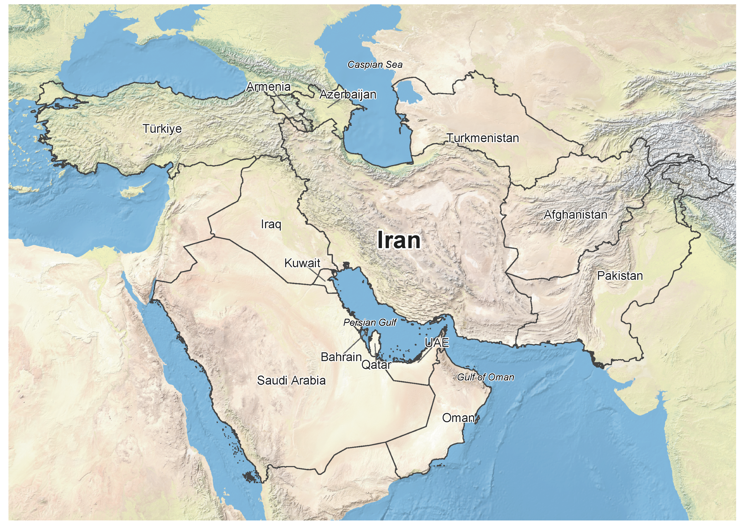
Figure 2.
Conceptual illustration of fractal-dimension estimation for Iran’s mainland boundary: (a) box-counting using boundary-intersecting boxes of side , and (b) the divider method using successive steps of length r. Insets enlarge representative boundary segments.
Figure 2.
Conceptual illustration of fractal-dimension estimation for Iran’s mainland boundary: (a) box-counting using boundary-intersecting boxes of side , and (b) the divider method using successive steps of length r. Insets enlarge representative boundary segments.
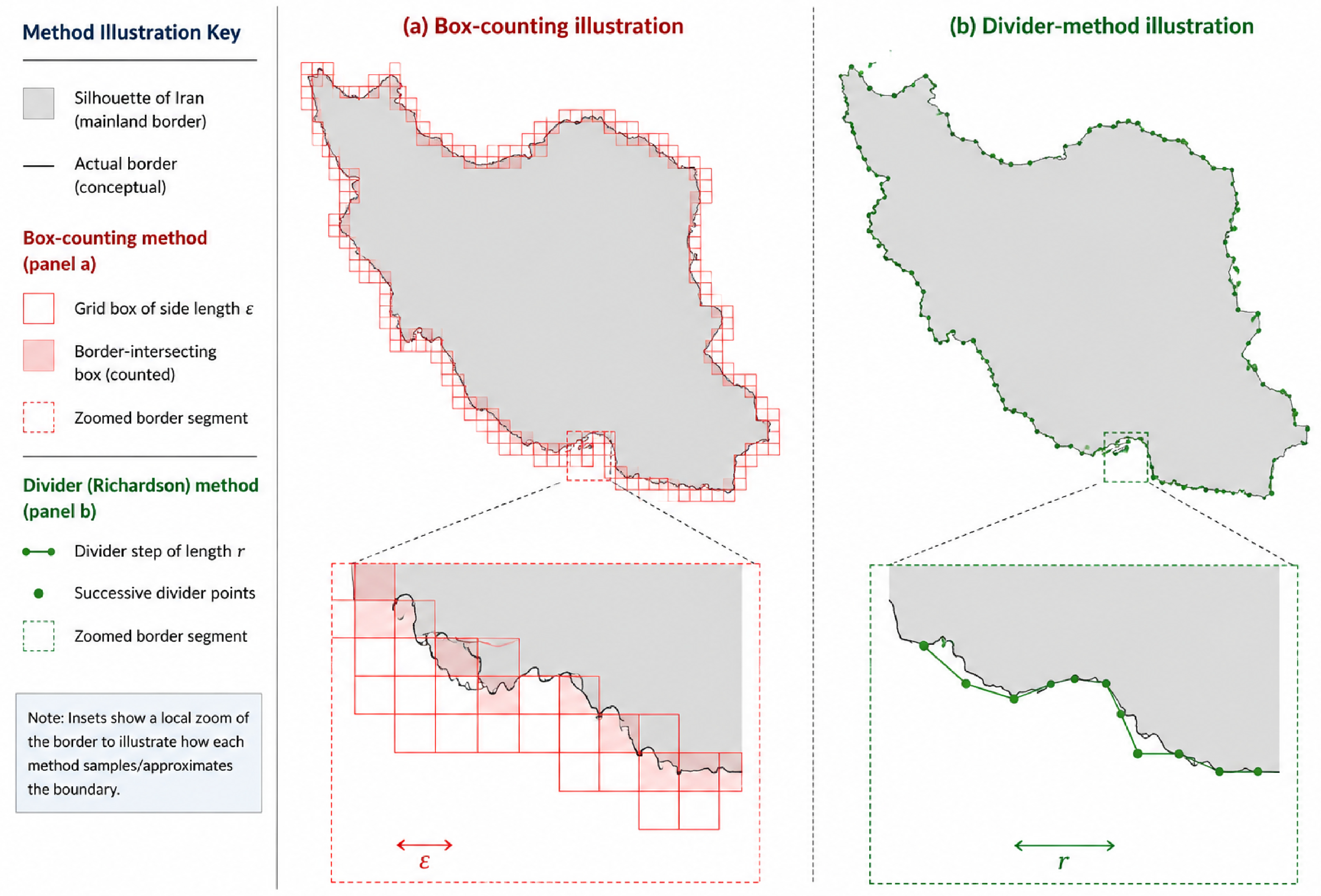
Figure 3.
West Asian comparison of box-counting and divider dimensions for modern Iran and 13 regional countries. The dashed line denotes , indicating cross-method agreement, while Iran is highlighted by a blue diamond.
Figure 3.
West Asian comparison of box-counting and divider dimensions for modern Iran and 13 regional countries. The dashed line denotes , indicating cross-method agreement, while Iran is highlighted by a blue diamond.
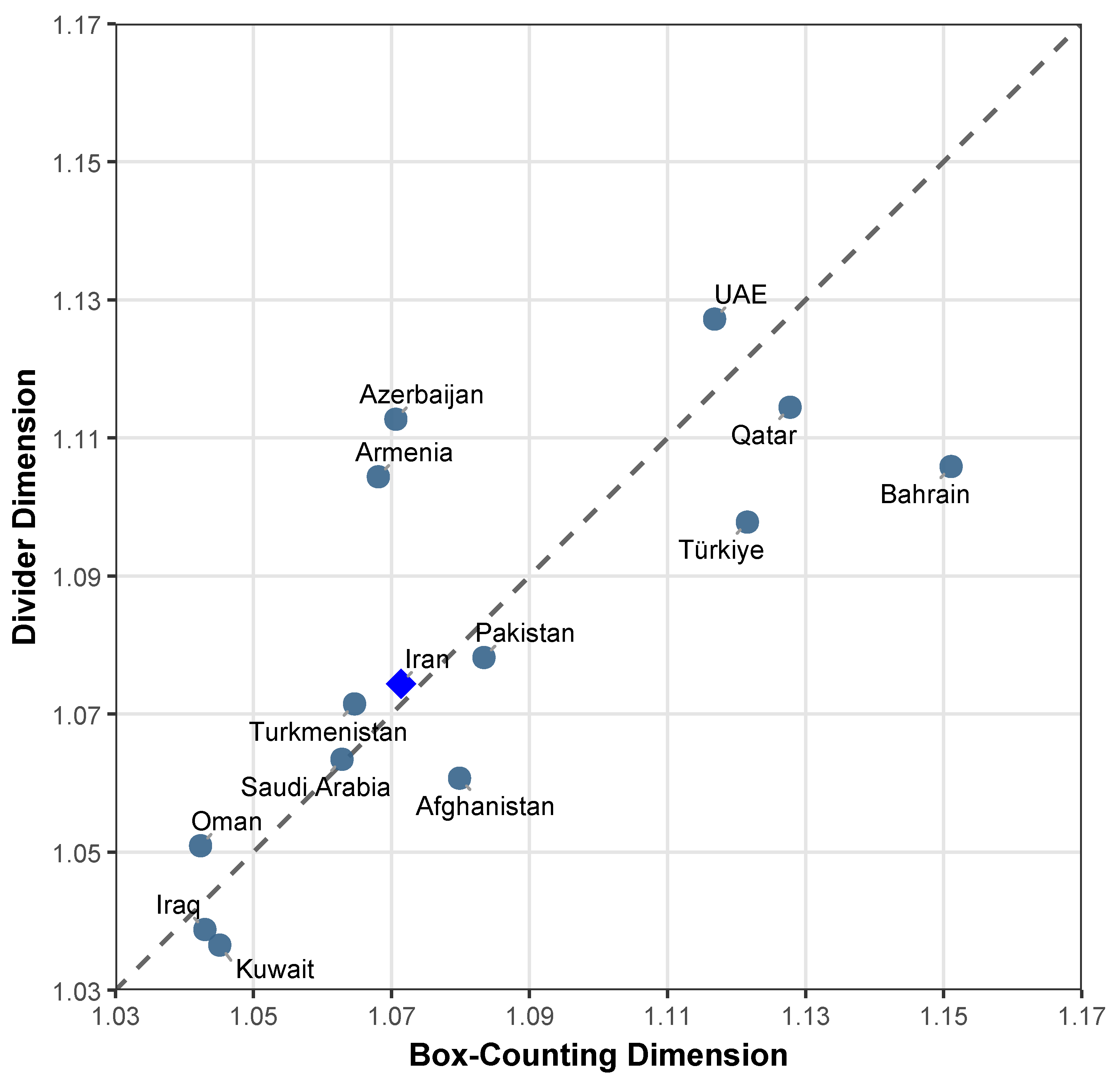
Figure 4.
Scaling regressions for Iran’s exterior border using (a) box-counting and (b) divider methods. Colored points denote selected scaling ranges, gray points excluded scales, and dashed lines the fitted regressions, yielding and .
Figure 4.
Scaling regressions for Iran’s exterior border using (a) box-counting and (b) divider methods. Colored points denote selected scaling ranges, gray points excluded scales, and dashed lines the fitted regressions, yielding and .
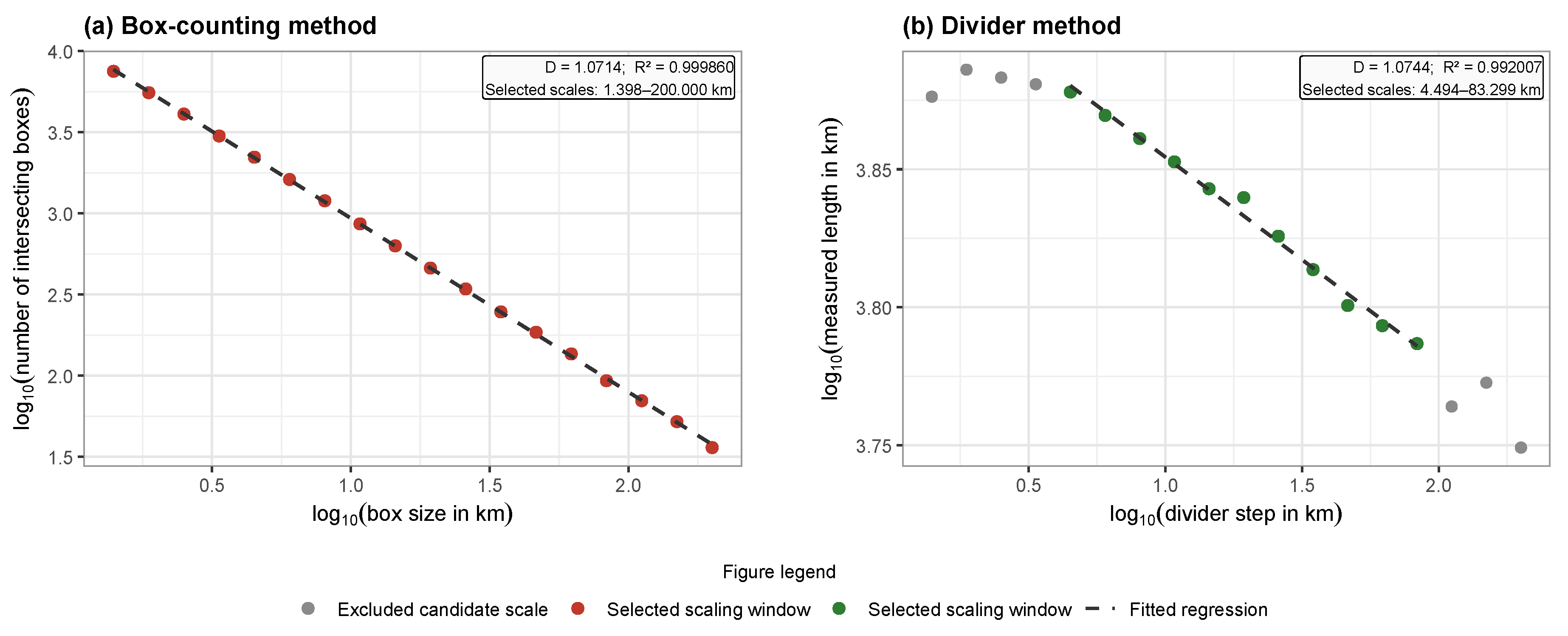
Figure 5.
Global comparison of published coastline fractal dimensions estimated by box-counting and divider methods. The dashed line denotes ; blue diamonds identify the Persian Gulf and Caspian Sea. Single-method studies are shown as faded equality-line projections with dotted guides.
Figure 5.
Global comparison of published coastline fractal dimensions estimated by box-counting and divider methods. The dashed line denotes ; blue diamonds identify the Persian Gulf and Caspian Sea. Single-method studies are shown as faded equality-line projections with dotted guides.
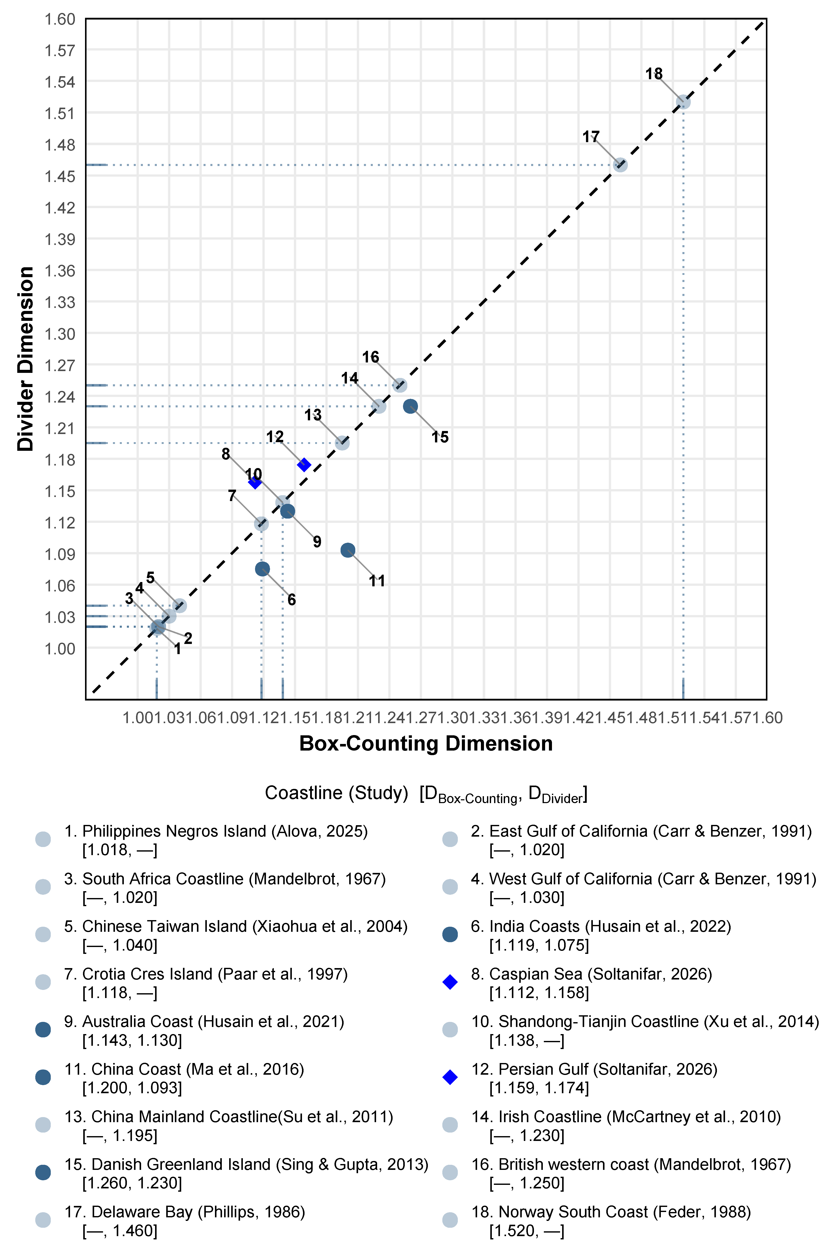
Disclaimer/Publisher’s Note: The statements, opinions and data contained in all publications are solely those of the individual author(s) and contributor(s) and not of MDPI and/or the editor(s). MDPI and/or the editor(s) disclaim responsibility for any injury to people or property resulting from any ideas, methods, instructions or products referred to in the content. |
© 2026 by the authors. Licensee MDPI, Basel, Switzerland. This article is an open access article distributed under the terms and conditions of the Creative Commons Attribution (CC BY) license (http://creativecommons.org/licenses/by/4.0/).
Copyright: This open access article is published under a Creative Commons CC BY 4.0 license, which permit the free download, distribution, and reuse, provided that the author and preprint are cited in any reuse.