

Submitted:
01 August 2026
Posted:
04 August 2026
You are already at the latest version
Abstract
Deep learning models often require a large number of parameters and computational resources, which can limit their deployment in resource-constrained or energy-sensitive environments. To address this challenge, we introduce the Separable Tensor Polynomial (STEP) layer, a framework that compresses deep learning architectures using low-rank tensorized polynomial expansions. STEP replaces dense layers and standard convolutional filters with structured, separable modules that maintain expressive power while drastically reducing parameter counts. The framework naturally supports 2D and 3D convolutional layers, tensorized activations, and other common network building blocks. We evaluated STEP extensively on classical high-dimensional function approximation, medical imaging benchmarks (MedMNIST, PneumoniaMNIST), Fashion-MNIST, and the Imagenette dataset. A single STEP layer is shown to replace multiple conventional dense or convolutional layers, achieving competitive or higher accuracy than deep architectures such as VGG16 [1] and ResNet50 [2] with parameter reductions of up to 99% in several experiments.By bridging approximation theory, tensor analysis, and modern deep learning, STEP offers a unified approach for building compact, expressive, and energy-efficient models. Its simple integration into existing networks and dramatic reductions in memory and computation make it particularly suitable for Green AI and edge deployment scenarios, enabling practical high-dimensional learning without relying on deep or over-parameterized architectures.
Keywords:
orthogonal polynomials
; tensor decomposition
; multivariable approximation
; explainable AI
; energy-efficient computation
1. Introduction
Deep neural networks (DNNs) are now one of the best tools for scientific computing, uncertainty quantification (UQ), and finding the numerical solution of partial differential equations (PDEs) [3,4]. They are very good at approximating high-dimensional nonlinear functions [5]. Their empirical success has been paralleled by a growing corpus of theoretical research that offers robust approximation assurances and elucidates how deep architectures can surmount the conventional curse of dimensionality that constrains classical numerical techniques. A significant area of research focuses on the expressive capacity of deep neural networks (DNNs) for parametric and countably-parametric partial differential equations (PDEs) [6,7]. In a groundbreaking study by Yarotsky et al., authors showed that deep ReLU networks can achieve dimension-independent approximation rates for generalized polynomial chaos (gPC) representations of holomorphic solution maps [8]. This proves that neural networks can effectively approximate complex models used in engineering and the physical sciences. These concepts were subsequently expanded to Bayesian inverse problems, such as Normalizing flow, wherein deep architectures yield dimension-independent approximation rates for posterior densities [9,10,11]
Figure 1.
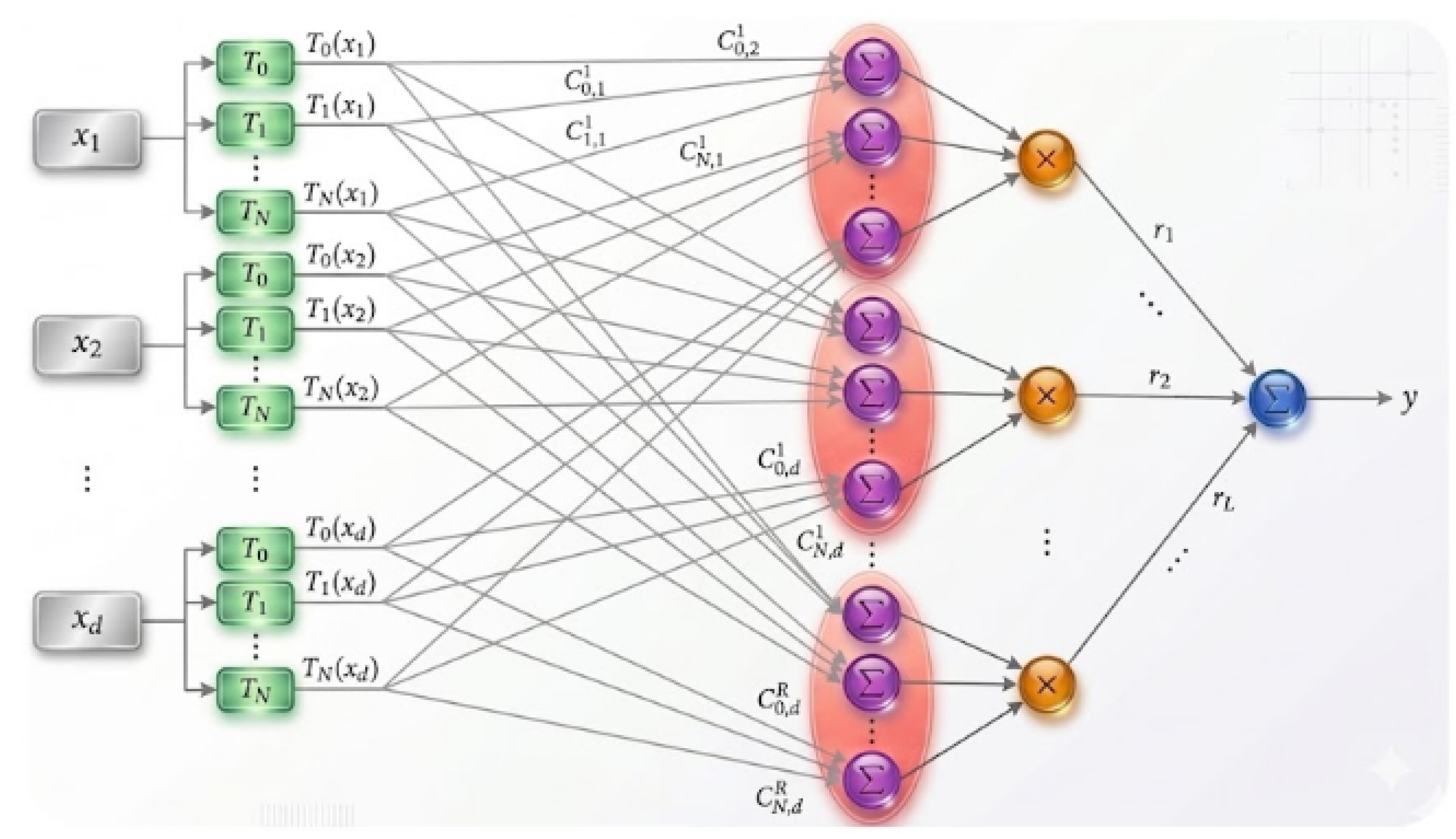
Schematic of the STEP architecture. Each component of the input is expanded in the Chebyshev basis . For each rank component , the layer forms one univariate polynomial per input variable and multiplies these polynomials across the d dimensions. The output is the sum of the R products, weighted by the scalars .
Figure 1.
Schematic of the STEP architecture. Each component of the input is expanded in the Chebyshev basis . For each rank component , the layer forms one univariate polynomial per input variable and multiplies these polynomials across the d dimensions. The output is the sum of the R products, weighted by the scalars .
From the perspective of approximation theory, it is now firmly established that depth fundamentally enhances expressive efficiency. Yarotsky [8] demonstrated that deep ReLU networks approximate smooth and continuous functions with near-optimal complexity, while the analyses in [12] established precise lower bounds and optimality results for deep and sparsely connected architectures. Later research showed that deep networks can match or beat the approximation rates of traditional affine representation systems like wavelets, curvelets, and shearlets [13,14]. This shows that they are good for structured function classes.
These advancements in approximation theory have significantly influenced the numerical resolution of high-dimensional partial differential equations (PDEs). A series of studies by Hutzenthaler, Jentzen, Grohs, and their associates [13,14], established that DNN-based solvers surmount the curse of dimensionality for semilinear Kolmogorov equations, Hamilton–Jacobi–Bellman equations, Black–Scholes PDEs, and nonlinear stochastic control problems. In these contexts, the quantity of network parameters necessary to attain a specified accuracy increases only polynomially with respect to the dimension and the inverse error tolerance, signifying a substantial enhancement over traditional discretization methods.
More theoretical work has been done, such as full training error analyses for stochastic gradient descent [15], space-time error estimates for deep PDE solvers [16], and the design of specialized architectures that take advantage of the structural properties of the problems at hand. Convolutional and tensorized networks [17,18,19] for parametric diffusion and transport equations [20] and links between high-dimensional quadrature strategies and neural approximation rates [21] are two examples. Polynomial-based spectral concepts have also impacted practical deep learning models; for example, [22] presented a Chebyshev-based convolutional neural network for lung cancer CT analysis, showcasing enhanced performance compared to conventional CNNs.
Even with these improvements, approximating functions in high dimensions remains challenging. Classical multivariate polynomial expansions require coefficients while fully connected neural layers require parameters (where N stands for the polynomial degree, d stands for data dimension and W stands for the network width). As a result, both methods become impractical in moderate to high dimensions. This drives the development of structured representations that keep their expressive power while significantly reducing the number of parameters. Related efforts have revisited the Kolmogorov–Arnold representation theorem, replacing fixed activations with learnable spline- or Chebyshev-parametrized edge functions [23,24], though these follow a different architectural design than the tensorized layer proposed here.
We propose a low-rank tensorized polynomial framework that yields explicit, scalable constructions compatible with modern deep architectures. Our method uses a simple, scalable architecture that fits well with modern deep learning design while dramatically reducing parameter complexity and still has strong theoretical guarantees offering a principled alternative to both dense neural layers and classical high-dimensional polynomial expansions. Table 1 shows a detailed comparison of representative orthogonal and structured convolutional layers highlighting the differences between the current methods and the proposed approach.
To deal with the computational and theoretical problems of current high-dimensional approximation methods, we present the Separable Tensor Polynomial (STEP) layer. This framework integrates low-rank tensor decomposition with Chebyshev spectral expansions to establish a Green AI [29] paradigm: attaining high-fidelity representations with significantly diminished depth, parameters, and energy consumption. The principal contributions of this study are encapsulated as follows:
- High-Efficiency "Green" Architecture: STEP uses a mode-separable structure that makes the number of parameters much simpler, going from the exponential of classical expansions to the linear . This lets STEP work as a "shallow-yet-deep" model, achieving accuracy that is competitive with deep networks while using up to fewer parameters. STEP captures global non-linear dependencies in a single layer by directly adding Chebyshev spectral representations to the neural activation path. This gets around the need for extreme depth and effectively reduces the "Curse of Dimensionality" in high-dimensional function approximation.
- Differentiable Tensor Interactions: We create a layer that can be differentiated natively and that does rank-separable interactions between spatial and spectral modes. This makes it possible to easily add STEP to modern architectures (like CNNs and dense networks) while keeping the theoretical rigor of low-rank tensor approximations. STEP offers verifiable convergence assurances that surpass the functionalities of conventional sparse grids and dense deep neural networks (DNNs). A comparative evaluation (see Table 1) shows that STEP is the only method that combines scalability, theoretical soundness, and compatibility with optimization based on gradients.
This work goes beyond the STEP as an architecture for shallow learning but rather to create a single mathematical framework for tensorized interactions that improves existing methods like sparse grids and polynomial expansions.
The remainder of this paper is organized as follows. In Section 2, we present the mathematical foundations of STEP, including its forward and backward passes as well as the spectral constructions. Section 3 focuses on theoretical evaluation with regards to complexity and error. Section 4 and Section 5 are where we formalize the experimental methodology and the empirical evaluation occurs respectively, focusing on shallow models, high-accuracy benchmarks, and energy efficiency. Finally, Section 6 concludes the paper with additional future work.
2. Proposed Method
The fully theory with all formal definitions and background required is presented here. In Appendix A we provide Table A1 which summarizes the notation used throughout the paper and in Appendix B, we present how the model parameters are learned.
2.1. Full Multivariate Chebyshev Expansion and Coefficient Tensor
Any function can be approximated by a truncated tensor-product Chebyshev expansion of maximum degree N:
We define the coefficient tensor of order d with mode size as
In subsequent subsections, we propose to approximate a high-dimensional function f by first computing its multivariate Chebyshev expansion and then applying a low-rank tensor decomposition.
2.2. Low-Rank Multivariate Approximation Using Chebyshev Tensor Decompositions
We propose to approximate the full coefficient tensor from (2) using a rank-R CP decomposition:
The resulting functional approximation of f is then given by:
where is the Chebyshev polynomial of degree i, is the range of variable , N is the same truncation order for each variable, are coefficients, is a scalar weight for component r, and R is the tensor rank. The total number of parameters reduces to , achieving significant compression when .
2.3. Tensor Formulation
We define the Chebyshev basis vector and their coefficient vector as the following, where from this point onwards we implicitly assume all inputs have been normalized to , absorbing the affine scaling from (4):
Then each inner sum becomes a dot product Thus (4) becomes
From the above, the full tensor product Chebyshev feature is defined as with their rank-1 coefficient tensor , then the approximation becomes
which is precisely the CANDECOMP/PARAFAC (CP) decomposition of a Chebyshev coefficient tensor.
2.4. Algorithm and Implementation Details
We describe the pseudocode in Algorithm 1 for the proposed method as follows:
| Algorithm 1 Low-Rank Functional Approximation via CP Decomposition |
|
2.5. STEP As Neural Network Layer
We propose a new layer defined by:
where is the expanded Chebyshev polynomial feature vector for dimension j, and are the learnable counterparts of the theoretical coefficient vectors in the earlier subsections, parameterizing the mode-j activation weight for rank r.
2.5.1. Forward/Backward Propagation
Given an input vector , the forward pass of the STEP layer proceeds as follows. First, each scalar input is expanded into its Chebyshev feature vector . For each rank component , we compute the separable product
where is the weight vector associated with input dimension j and rank r. The total pre-activation is obtained by summing over all rank components:
Finally, the layer output is produced by applying a non-linear activation function :
This formulation explicitly decouples the interactions across dimensions via the low-rank structure, yielding a parameter count that scales linearly with the input dimension d, the polynomial degree N, and the rank R, rather than exponentially.
We now discuss backward propagation. Let denote the derivative of the activation function. The gradient with respect to is:
2.6. STEP Embedding Layer
The STEP-Embedding mechanism regularizes the token representation space through a spectral bottleneck. The forward mapping is defined as:
where [30] denotes the standard token embedding lookup and is the fixed Chebyshev basis matrix. By forcing the embedding through an R-dimensional manifold , the architecture filters out high-frequency noise inherent in high-dimensional dense embeddings.
3. Theoretical Performance and Complexity
In this section we analyze the proposed method’s properties of convergence, error, and complexity. We also apply it to specific models, and try to justify its efficiency using the proposed method.
3.1. STEP Framework
3.1.1. Convergence Analysis
In Appendix C we present a hierarchical analysis of the approximation error, decomposing it into contributions from polynomial truncation and tensor rank reduction. Here we state the main Theorem which ensures convergence of the model,
Theorem 1
(Two-Stage Convergence). Let . For the approximation defined by the low-rank Chebyshev model,
Furthermore, if f is analytic, the convergence with respect to N is exponential.
3.1.2. Error Analysis
We now analyze the total approximation error of the low-rank tensor Chebyshev expansion by decomposing it into two distinct components: the spectral truncation error and the low-rank CP approximation error.
Theorem 2
(Error Decomposition). Let , let be its N-truncated tensor Chebyshev expansion, and let be the rank-R CP approximation. If f is analytic in a Bernstein ellipse of radius , and bounded by the best rank-R approximation of the coefficient tensor, then the total error is bounded by .
Proof.
By the triangle inequality:
□
Remark: If f has bounded mixed partial derivatives up to order s, or is analytic in a Bernstein ellipse of radius , then we have:
Furthermore, if the tensor rank error is bounded by the best rank-R approximation error of the coefficient tensor, then we have:
3.1.3. Complexity Analysis
Table 2 compares the computational complexity for function evaluation between the classical full tensor method and the proposed low-rank approach. The classical method exhibits exponential complexity of , whereas the proposed method reduces this to , which is linear in both dimension d and polynomial degree N. The complexity ratio,
demonstrates an exponential gain in favor of the low-rank approximation, particularly for high-dimensional problems. This reduction in complexity makes the proposed approach well-suited for applications where d is large and fast function evaluations are required.
3.2. STEP Neural Network Layer
It is noted that the STEP layer from (7) has a parameter count:
where denotes the length of the expanded feature vector. The layer performs a mapping , where the pre-activation is computed through two distinct stages:
- 1.
- Spectral Expansion: Given input , we first apply Min-Max normalization to map to the domain , followed by the Chebyshev lifting:
- 2.
- Low-Rank Projection: The spectral features are compressed through a rank-R bottleneck defined by learnable factors and :
This composition reduces the parameter count from in a standard dense layer to .
4. Experimental Methodology
We conduct a comprehensive study spanning classical high-dimensional function approximation and modern convolutional neural network architectures. The experiments are designed to highlight STEP’s ability to drastically reduce parameter count and computational cost while maintaining or improving accuracy relative to full-rank, conventional, and deep benchmark models.
For each benchmark function or network architecture, we perform the following systematic analysis:
- 1.
- Function or Model Definition: We formally define the target function or the CNN architecture under study. For functions, we outline their domain and classical full-tensor polynomial expansion. For CNNs, we specify the baseline kernel size, layer configuration, and dataset such as MNIST [31].
- 2.
- STEP Construction and Low-Rank Analysis: We construct the low-rank tensorized approximation or decomposed convolutional filters using CP decomposition or mode-wise separable factorization. The decay of CP weights () or singular modes is analyzed to justify the selected rank R.
- 3.
-
Comparative Performance Metrics:
- Accuracy Comparison: Quantitative evaluation of approximation errors for functions () and classification accuracy for CNNs. Comparisons include full-rank expansions, sparse grids, Tensor-Train decompositions, and baseline deep models.
- Efficiency Comparison: Metrics include parameter count, storage requirements, and computational cost (operations per evaluation, multiplications/additions per pixel or voxel). Tables summarize gains achieved through low-rank tensorization.
- 4.
- Summary of Findings: For each experiment, we highlight the minimum rank R required to achieve target accuracy, quantify compression and speedup factors, and discuss implications for shallow STEP networks, Green AI deployment, and high-dimensional learning efficiency.
This structured approach ensures that all experiments, from smooth function approximation to CNN compression and benchmark deep networks, are analyzed consistently. The results empirically confirm the theoretical advantages of STEP in reducing computational complexity while preserving or enhancing predictive accuracy.
5. Results
This section provides a rigorous empirical validation of the Separable Tensor Polynomial (STEP) framework. Additional results, namely the evolution of validation accuracy over training epochs together with model size and CPU inference latency for each experiment, are available in Appendix D, which highlights the stability of STEP over training.
5.1. STEP For Function Approximation
In this section, we provide a unified presentation of illustrative examples demonstrating the power of tensorized polynomial approximations using the STEP framework.
We use the following functions below and try to approximate them with STEP.
- 1.
- Function 1 (2D):, rank .
- 2.
- Function 2 (3D):, smooth radial function; classical vs STEP .
- 3.
- Function 3 (4D):, rank .
For each function, we include: definition, classical approximation, tensorized approximation construction, error comparison tables, and discussion.
From the above Table 3, we can see that across all examples, the STEP framework consistently demonstrates parameter efficiency as it dramatically reduces parameters compared to the full tensor approximations. Along with this is the increased precision as for both low and moderate dimensional functions, small errors can be achieved even if the rank R is small. We also note the advantages of scalability as higher dimensions require parameters without exponential growth and the ability to control accuracy through increasing the rank R which implies that the framework works for deep learning models.
5.2. STEP vs Traditional MLP
This section evaluates STEP model using the formulation discussed in Section 3.2 on two different datasets: a synthetic function dataset, and the Fashion-MNIST [32] dataset converted into a 1D representation. These datasets represent different levels of complexity, including nonlinear functional learning, structured mathematical patterns, and real-world image classification.
The workflow is shown in Figure 2 for clarity of the experiment. For a fair comparison, the traditional MLP and the STEP-based MLP are trained under identical experimental conditions in terms of epochs and dataset splits. While the traditional MLP relies on fully connected dense layers, the STEP model replaces the integration stage with a spectral tensorized projection that significantly reduces the number of parameters while maintaining competitive accuracy. We observe throughout the experiments here that (1) we can model high dimensional nonlinear interactions with a parameter count that scales linearly with dimension d and rank R, avoiding the exponential blow-up typical of full tensors, (2) gradients are explicitly defined, ensuring STEP integrates seamlessly with standard optimization routines, even in large-scale high-dimensional settings allowing for drop in replacements to standard models, (3) STEP embodies Green AI principles by substantially reducing memory and energy demands while maintaining strong predictive accuracy, making it highly suitable for resource-constrained and edge deployment scenarios.
5.2.1. Experiment 1: Function Dataset
The first experiment evaluates both models on a nonlinear synthetic function dataset defined as:
Purely from a function approximation perspective, we see that STEP better captures its shape due to higher validation accuracy and doesn’t fit to noise as much compared to the MLP in Table 4. This also hints that deep learning models easily overfit in terms of parameter size and STEP provides a concrete answer to parameter efficiency without either overfitting or underfitting.
5.2.2. Experiment 2: Fashion-MNIST (Converted to 1D)
In the second experiment, the models are evaluated on the Fashion-MNIST dataset after converting the images into a 1D representation.
Here, STEP demonstrates again its parameter efficiency in Table 5. It uses 5% of parameters of the MLP while having comparable validation accuracy. Due to the reduction in parameters, inference speed has increased slightly, in further experiments in the next section, we demonstrate the speedup is significant for larger models in the parameter sizes up to millions.
5.3. STEP vs. Traditional CNN
This section presents a controlled comparison between the (STEP) model and a traditional Convolutional Neural Network (CNN) using the MedMNIST [33], PneumoniaMNIST, and Imagenette [34] datasets. Models are trained under identical experimental conditions to ensure a fair and unbiased comparison in terms of accuracy, model complexity, and computational efficiency.
The main difference between the two models lies in the integration mechanism. While the traditional CNN relies on spatial flattening followed by dense fully connected layers, the STEP model replaces this stage with localized spectral projection using Chebyshev polynomial filters defined on the interval as shown in Figure 3.
5.3.1. Experiment 1: MedMNIST Dataset (Epoch 15)
The first experiment evaluates the performance of the STEP model compared with a traditional CNN on the MedMNIST dataset after 15 training epochs.
Running on the MedMNIST dataset, we see in Table 6 the potential for real-time applications with large models as we can have comparable accuracy while only using 10% of the parameters. In addition to this, latency is halved, further supporting the use of STEP in embedded devices due to reduced memory and latency.
5.3.2. Experiment 2: PneumoniaMNIST Dataset (Epoch 15)
To further evaluate the robustness of the STEP architecture, we compare it with traditional deep learning models on the PneumoniaMNIST dataset.
From Table 7, the STEP model is smaller by a wide margin than every baseline against which it is compared. This is especially prevalent in the case where we compare STEP against ResNet50, where STEP is over 550× smaller while achieving higher accuracy (0.8333 vs. 0.8077); it also slightly outperforms the Traditional CNN at less than a ninth of its size. The only case where accuracy is significantly lower is for the VGG16 model, but it should be noted that STEP is 346.7x smaller so there has to be a tradeoff between efficiency and performance to some degree.
5.3.3. Experiment 3: Imagenette Dataset (Epoch 10)
To evaluate scalability, we extend the comparison to the Imagenette dataset using models trained from scratch.
From the Table 8 above, STEP’s shallow tensorized architecture attains competitive accuracy relative to deeper and heavily parameterized models like VGG16 and ResNet50. Remarkably, STEP uses orders of magnitude fewer parameters (126k vs 24.1M for ResNet50) while maintaining superior validation accuracy (0.586 vs 0.308 at Epoch 10), demonstrating that depth and parameter count are not strictly necessary to achieve high performance when expressive spectral representations are employed.
5.3.4. Experiments 4 & 5: Hybrid VGG16-STEP and ResNet50-STEP on the Imagenette Dataset
This section evaluates the STEP layer integrated into VGG16 and ResNet50 architectures on the Imagenette dataset. The goal is to assess how spectral tensor expansion reduces model complexity while maintaining classification performance across different deep architectures.
Similar to the previous subsection, incorporating STEP layers maintains accuracy as shown in Table 9 as shown in the comparison between the Hybrid and Standard VGG16 while reducing the parameter size up to half. The comparison between Hybrid and Standard ResNet50 is in contrast as it shows extreme compression with only roughly 10% of the original parameters while performing competitively, it is noted that the latency is significantly reduced due to the parameter reduction.
5.4. STEP VS LLM Tokenizer Generations
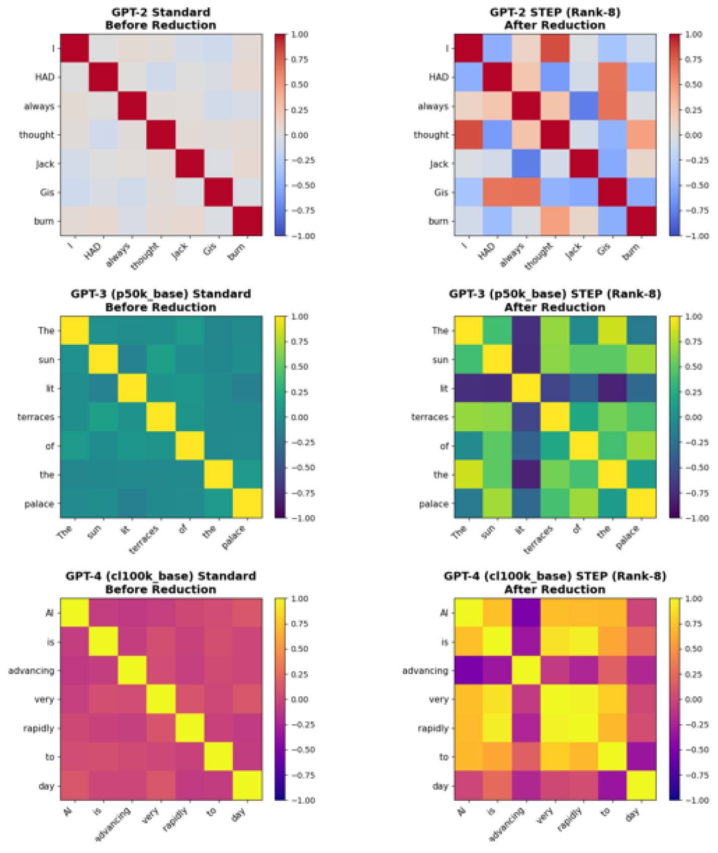
To evaluate the scalability and robustness of the STEP architecture, we benchmark the STEP-Embedding layer against standard dense embedding matrices across three sizes of Large Language Model tokenizers [35]: GPT-2 [36] size tokenizer (vocab size: 50,257), GPT-3 [37] p50k_base size tokenizer (vocab size: 50,281), and GPT-4 cl100k_base size tokenizer (vocab size: 100,277). The target embedding dimension was held constant at 256. We analyzed both parameter efficiency and geometric fidelity. This projection from (8) acts as a structural regularizer, preserving the semantic identity of tokens while achieving parameter reduction. As shown in the workflow of Figure 4, we set a low rank bottleneck for compression. Appendix E provides a graphical understanding of how the embedding space is affected.
The traditional embedding approach scales linearly with vocabulary size, resulting in severe parameter bloat. For the GPT-4 size tokenizer, the standard dense matrix requires over 25.6 million parameters just for the input layer. By routing the token identities through an 8-dimensional Chebyshev manifold, the STEP architecture achieved a massive reduction in memory footprint across all generations, consistently exceeding compression (see Table 10). A primary concern with extreme bottleneck compression is the loss of token identity (linear collapse). To test this, we performed a reverse-decoding proof using Nearest-Neighbor Euclidean Distance ( Norm) to map the outputted 256-dimensional continuous vectors back to the discrete vocabulary space. Across diverse grammatical structures and all model generations, the STEP Rank-8 layer achieved a string-match reconstruction rate as shown in Table 10. This empirically shows that the inner-manifold Mish activation [38] prevents structural amnesia and preserves absolute semantic identity.
6. Conclusions
This work introduced the Separable Tensor Polynomial (STEP) framework, a principled approach for low-rank tensorized polynomial expansions in both function approximation and deep learning. STEP overcomes the classical curse of dimensionality by employing structured tensor decompositions, reducing parameter growth from exponential to linear in the dimension () while maintaining high approximation fidelity. Further experiments on the Imagenette dataset confirmed that shallow STEP models achieve competitive validation accuracy relative to deeper architectures such as VGG16 and ResNet50, while using orders of magnitude fewer parameters (126k vs. 24.1M for ResNet50) and lower inference latency. Integrated directly into these architectures, STEP reduces parameter counts by up to 91.8% while preserving over 97% of classification accuracy. Notably, a single STEP layer consistently replaces multiple conventional dense or convolutional layers across experiments, with very few trainable parameters relative to traditional baselines, confirming that a shallow architecture need not sacrifice competitive performance. These results demonstrate that STEP provides a powerful mechanism for model compression, accelerated computation, and energy-efficient deployment, making it highly suitable for resource-constrained and Green AI scenarios. Future work will focus on extending STEP to larger datasets, exploring adaptive rank selection, integrating with pruning and quantization [39], and assessing its deployment efficiency in edge AI environments.
Appendix A. Summary of Notation

Table A1.
Comprehensive Notation and Parameter Definitions
| Symbol / Variable | Definition |
|---|---|
| Function Approximation & Dimensions | |
| Multivariate input vector | |
| d | Total number of variables (input dimensions) |
| j | Index identifying the variable/dimension () |
| True continuous multivariate function mapping | |
| Model approximation of the function using CP-Chebyshev | |
| R | Maximum tensor rank (number of CP components) |
| r | Index identifying the tensor rank component () |
| Scalar magnitude (weight) of the r-th rank component | |
| Chebyshev Polynomials & Tensor Decompositions | |
| ⊗ | Tensor (outer) product operator resulting in higher-order tensors from lower-order tensors. Example: |
| N | Maximum degree of the Chebyshev polynomials (truncation order) |
| i | Index identifying the polynomial degree () |
| The i-th Chebyshev polynomial of the first kind | |
| Theoretical range scaling constant for variable | |
| Chebyshev scalar coefficient corresponding to degree i, variable j, and component r | |
| Column vector of Chebyshev coefficients | |
| Column vector of evaluated Chebyshev basis | |
| Rank-1 coefficient tensor corresponding to the r-th component | |
| Full tensor product of Chebyshev features across all d dimensions | |
| The full (uncompressed) order-d coefficient tensor truncated at degree N | |
| Scalar element of the full coefficient tensor | |
| The rank-R CP approximated coefficient tensor | |
| Multi-index indicating the polynomial degrees across all d dimensions | |
| Data matrices & ALS Optimization | |
| M | Total number of data samples |
| k | Index identifying a specific data sample () |
| Chebyshev design matrix evaluating all M samples across degrees for variable j | |
| Intermediate 1D polynomial approximation for variable j, component r, sample k | |
| Product of evaluations in all dimensions except j for sample k, component r | |
| Diagonal weight matrix formed by elements across all M samples | |
| L | Mean-squared-error (MSE) loss between true values and approximations |
| Vector of observed outputs | |
| Convergence Theory | |
| Orthogonal product weight function over the domain | |
| Radius of the Bernstein polyellipse governing the exponential convergence rate | |
| s | Order of bounded mixed partial derivatives |
| STEP Activation Layer | |
| Mode-j activation weight vector for rank r | |
| Separable dot product for rank component r | |
| z | Total pre-activation sum |
| Non-linear activation function | |
| Derivative of the activation function | |
| y | Final output of the STEP layer |
Appendix B. Estimation of Parameters
Given M samples for , we construct the Chebyshev design matrix for each variable j, where its elements are defined by . We then define the intermediate variable , which allows the approximation to be expressed as a summation over rank-R terms: . We now define the estimation of parameters through the use of alternating least squares and backpropagation.
Appendix B.1. Alternating Least Squares
We aim to minimize the mean-squared-error loss between the true values and their approximations :
The optimization is performed via an alternating least-squares (ALS) scheme. At each step, we update the coefficient vector for a single variable j and rank index r while keeping all other coefficients fixed. To isolate its contribution, we define the intermediate quantity
which collects the product of all other terms in the rank-r component. The model approximation can then be rewritten linearly in the target coefficients as
Let be the vector of observed outputs and define the diagonal weight matrix for each r. Substituting the linearized form into the loss L yields a weighted least-squares problem for , with the solution
where is the Chebyshev design matrix for variable j defined previously. Iterating this update cyclically over all j and r constitutes a standard ALS algorithm for fitting the model.
Appendix B.2. Gradient-Based Optimization
The model is differentiable, and
applying the chain rule. This allows optimization via Adam, RMSprop, or L-BFGS.
Appendix C. Convergence Analysis
It is well-known that for continuous functions f on , then the Chebyshev series converges in [40].
Moreover, for analytic functions on a Bernstein ellipse, the truncation error decays exponentially [41].
and the multivariate tensor expansion satisfies the exponential bound
which still decays exponentially in N. The rank R controls the ability to represent non-separable interactions. If f has minimal tensor rank , then the approximation converges to f whenever .
Appendix C.1. Orthogonal Basis and Series Expansion
The Chebyshev tensor basis functions, defined for a multi-index as
form a complete orthogonal system in the weighted space with the product weight . Consequently, any function admits a unique expansion
which converges in the norm.
Appendix C.2. Spectral Convergence of Polynomial Truncation
Truncating the series to maximum degree N in each variable yields the approximation
This truncation is the orthogonal projection onto the subspace of polynomials of degree at most N, guaranteeing that as . The convergence rate depends on the smoothness of f:
- If f has s continuous derivatives, the error decays algebraically: .
- If f is analytic on a Bernstein polyellipse, the error decays exponentially: there exists such that .
Appendix C.3. Low-Rank Tensor Approximation
Let denote the coefficient tensor of . To circumvent the exponential growth of terms, we employ a rank-R CANDECOMP/PARAFAC (CP) approximation . A fundamental property of the CP format is that any finite tensor can be approximated arbitrarily well with sufficient rank, i.e.,
Since the norm of the corresponding function approximation is controlled by the Frobenius norm of the coefficient tensor, we have
Appendix C.4. Total Error Decomposition and Main Result
The total approximation error decomposes via the triangle inequality:
The first term vanishes as the polynomial degree N increases, and the second term vanishes as the tensor rank R increases. This leads to our main convergence guarantee in Theorem 1.
Appendix D. Training Curves and Efficiency Comparisons
Figure A1.
MedMNIST (Table 6): validation accuracy over epochs, model size, and CPU inference latency for STEP versus the traditional CNN.
Figure A1.
MedMNIST (Table 6): validation accuracy over epochs, model size, and CPU inference latency for STEP versus the traditional CNN.
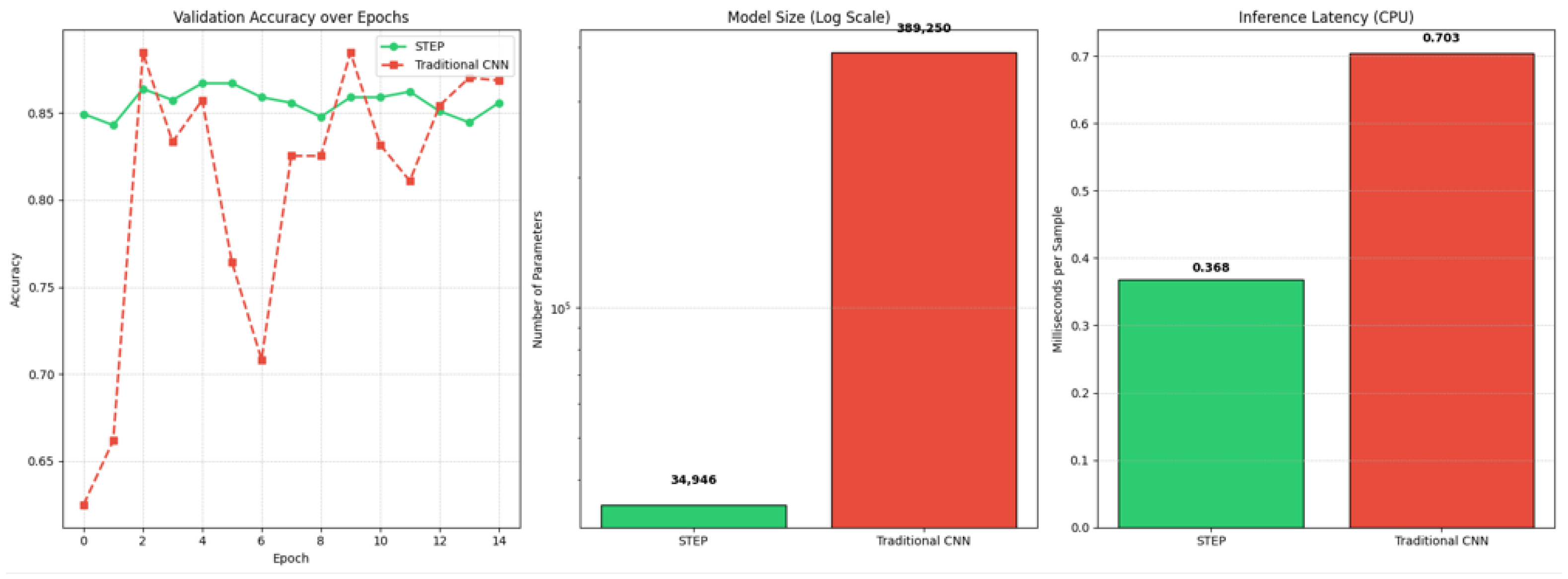
Figure A2.
PneumoniaMNIST (Table 7): validation accuracy over epochs, model size, and CPU inference latency for STEP versus the traditional CNN, VGG16, and ResNet50.
Figure A2.
PneumoniaMNIST (Table 7): validation accuracy over epochs, model size, and CPU inference latency for STEP versus the traditional CNN, VGG16, and ResNet50.
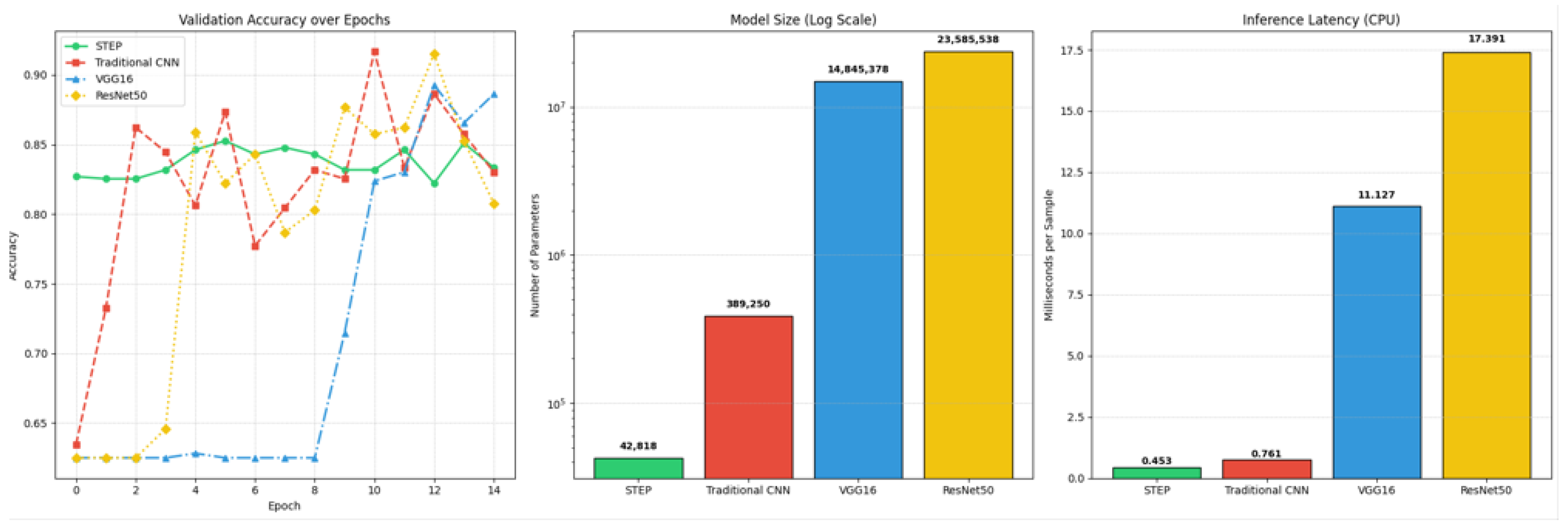
Figure A3.
Imagenette, all models trained from scratch (Table 8): validation accuracy over epochs, model size, and CPU inference latency. VGG16 fails to leave random-guess accuracy under this training budget.
Figure A3.
Imagenette, all models trained from scratch (Table 8): validation accuracy over epochs, model size, and CPU inference latency. VGG16 fails to leave random-guess accuracy under this training budget.
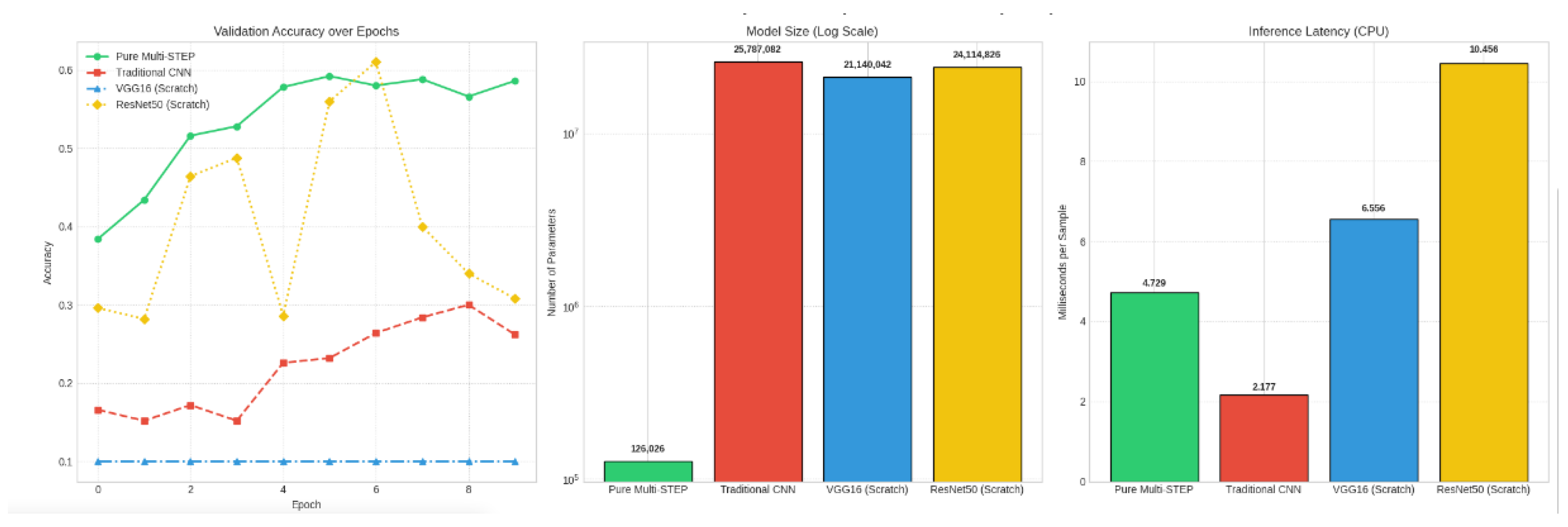
Figure A4.
Hybrid VGG16-STEP versus standard VGG16 on Imagenette with two-stage training (Table 9): validation accuracy over epochs, model size, and CPU inference latency. The dashed line marks the start of deep fine-tuning.
Figure A4.
Hybrid VGG16-STEP versus standard VGG16 on Imagenette with two-stage training (Table 9): validation accuracy over epochs, model size, and CPU inference latency. The dashed line marks the start of deep fine-tuning.
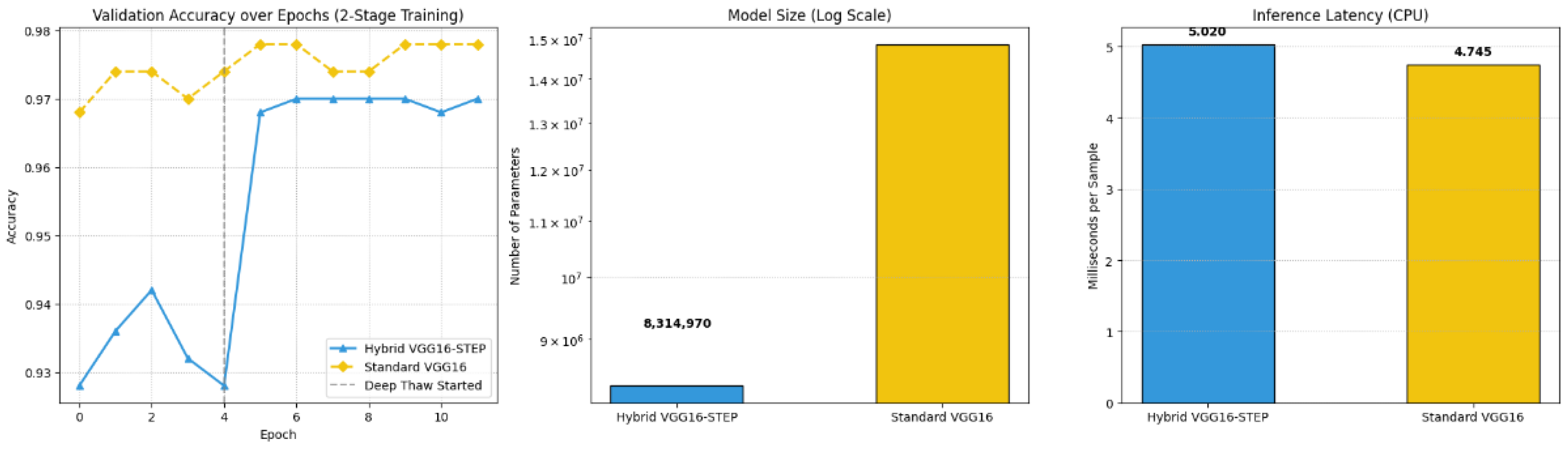
Figure A5.
Hybrid ResNet-STEP versus standard ResNet50 on Imagenette (Table 9): validation accuracy over epochs, model size, and CPU inference latency.
Figure A5.
Hybrid ResNet-STEP versus standard ResNet50 on Imagenette (Table 9): validation accuracy over epochs, model size, and CPU inference latency.
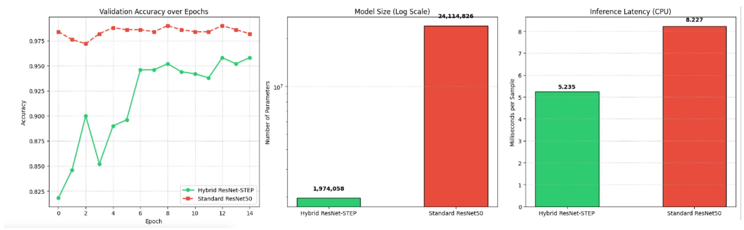
Figure A6.
Token Embedding Correlation Across LLM Generations (GPT-2 to GPT-4).
This appendix collects, for each classification experiment in Section 5, the evolution of validation accuracy over training epochs together with the model size (log scale) and the CPU inference latency per sample. Across all experiments, STEP shows stable accuracy from the earliest epochs, in contrast to the larger fluctuations of the dense baselines.
Appendix E. Step VS LLM Tokenizer Correlation Visualization
In here we show the effect of the correlation between some tokens in the embedding space demonstrating the effect of applying STEP to the space graphically. The standard matrices (left column) contain up to 25.6M parameters, allowing for spurious correlation noise between tokens. The STEP matrices (right column) achieve over 96% parameter reduction, retaining only essential spectral features while fully preserving decoding fidelity.
References
- Simonyan, K.; Zisserman, A. Very deep convolutional networks for large-scale image recognition. arXiv preprint arXiv:1409.1556 2014.
- He, K.; Zhang, X.; Ren, S.; Sun, J. Deep residual learning for image recognition. In Proceedings of the Proceedings of the IEEE conference on computer vision and pattern recognition, 2016, pp. 770–778.
- Schwab, C.; Zech, J. Deep learning in high dimension: Neural network expression rates for generalized polynomial chaos expansions in UQ. Analysis and Applications 2019, 17, 19–55. [CrossRef]
- Opschoor, J.A.; Petersen, P.C.; Schwab, C. Deep ReLU networks and high-order finite element methods. Analysis and Applications 2020, 18, 715–770. [CrossRef]
- Han, J.; Jentzen, A.; E, W. Solving high-dimensional partial differential equations using deep learning. Proceedings of the National Academy of Sciences 2018, 115, 8505–8510. [CrossRef]
- Kutyniok, G.; Petersen, P.; Raslan, M.; Schneider, R. A theoretical analysis of deep neural networks and parametric PDEs. Constructive Approximation 2022, 55, 73–125. [CrossRef]
- Petersen, P.; Voigtlaender, F. Optimal approximation of piecewise smooth functions using deep ReLU neural networks. Neural Networks 2018, 108, 296–330. [CrossRef]
- Yarotsky, D. Error bounds for approximations with deep ReLU networks. Neural networks 2017, 94, 103–114. [CrossRef]
- Cui, T.; Law, K.J.H.; Marzouk, Y.M. Dimension-Independent Likelihood-Informed Markov Chain Monte Carlo. Journal of Computational Physics 2016, 304, 109–137.
- Papamakarios, G.; Pavlakou, T.; Murray, I. Masked Autoregressive Flow for Density Estimation. In Proceedings of the Advances in Neural Information Processing Systems, 2017.
- Rezende, D.J.; Mohamed, S. Variational Inference with Normalizing Flows. In Proceedings of the Proceedings of the 32nd International Conference on Machine Learning, 2015.
- Yarotsky, D. Optimal approximation of continuous functions by very deep ReLU networks. In Proceedings of the Conference on learning theory. PMLR, 2018, pp. 639–649.
- Grohs, P.; Kutyniok, G.; Petersen, P.; Raslan, M.; Schneider, R. Deep Neural Network Approximation Theory. Journal of Machine Learning Research 2019, 19, 1–46.
- Grohs, P.; Hornung, F.; Jentzen, A.; Von Wurstemberger, P. A proof that artificial neural networks overcome the curse of dimensionality in the numerical approximation of Black–Scholes partial differential equations; Vol. 284, Memoirs of the American Mathematical Society, American Mathematical Society, 2023. [CrossRef]
- Robbins, H.; Monro, S. A Stochastic Approximation Method. The Annals of Mathematical Statistics 1951, 22, 400–407.
- Ghadimi, S.; Lan, G. Stochastic First- and Zeroth-Order Methods for Nonconvex Stochastic Programming. SIAM Journal on Optimization 2013, 23, 2341–2368. [CrossRef]
- Oseledets, I.V. Tensor-train decomposition. SIAM Journal on Scientific Computing 2011, 33, 2295–2317. [CrossRef]
- Novikov, A.; Podoprikhin, D.; Osokin, A.; Vetrov, D.P. Tensorizing neural networks. Advances in neural information processing systems 2015, 28.
- Lebedev, V.; Ganin, Y.; Rakhuba, M.; Oseledets, I.; Lempitsky, V. Speeding-up convolutional neural networks using fine-tuned cp-decomposition. arXiv preprint arXiv:1412.6553 2014.
- Kutyniok, G.; Petersen, P.; Raslan, M.; Schneider, R. A Theoretical Analysis of Deep Neural Networks and Parametric PDEs. Constructive Approximation 2019, 49, 1–53.
- Grohs, P.; Kutyniok, G.; Petersen, P. Deep Neural Networks for Approximation of Piecewise Smooth Functions. Analysis and Applications 2022.
- Bach, F. Breaking the Curse of Dimensionality with Convex Neural Networks. Journal of Machine Learning Research 2017, 18, 1–53.
- Liu, Z.; Wang, Y.; Vaidya, S.; Ruehle, F.; Halverson, J.; Soljacic, M.; Hou, T.; Tegmark, M. KAN: Kolmogorov–arnold networks. In Proceedings of the International conference on learning representations, 2025, Vol. 2025, pp. 70367–70413.
- SS, S.; AR, K.; KP, A.; et al. Chebyshev polynomial-based kolmogorov-arnold networks: An efficient architecture for nonlinear function approximation. arXiv preprint arXiv:2405.07200 2024.
- Novak, E.; Wozniakowski, H. Tractability of multivariate problems; EMS Press, 2008.
- Bungartz, H.J.; Griebel, M. Sparse grids. Acta numerica 2004, 13, 147–269.
- Gu, Y.; Ng, M.K. Deep Ritz Method for the Spectral Fractional Laplacian Equation Using the Caffarelli–Silvestre Extension. SIAM Journal on Scientific Computing 2022, 44, A2018–A2036. [CrossRef]
- Grasedyck, L.; Kressner, D.; Tobler, C. A literature survey of low-rank tensor approximation techniques. GAMM-Mitteilungen 2013, 36, 53–78. [CrossRef]
- Schwartz, R.; Dodge, J.; Smith, N.A.; Etzioni, O. Green ai. Communications of the ACM 2020, 63, 54–63.
- Vaswani, A.; Shazeer, N.; Parmar, N.; Uszkoreit, J.; Jones, L.; Gomez, A.N.; Kaiser, Ł.; Polosukhin, I. Attention is all you need. Advances in neural information processing systems 2017, 30.
- LeCun, Y.; Bottou, L.; Bengio, Y.; Haffner, P. Gradient-based learning applied to document recognition. Proceedings of the IEEE 1998, 86, 2278–2324. [CrossRef]
- Xiao, H.; Rasul, K.; Vollgraf, R. Fashion-mnist: a novel image dataset for benchmarking machine learning algorithms. arXiv preprint arXiv:1708.07747 2017.
- Yang, J.; Shi, R.; Wei, D.; Liu, Z.; Zhao, L.; Ke, B.; Pfister, H.; Ni, B. Medmnist v2-a large-scale lightweight benchmark for 2d and 3d biomedical image classification. Scientific data 2023, 10, 41. [CrossRef]
- Howard, J. Imagenette: A smaller subset of 10 easily classified classes from Imagenet, 2019.
- Sennrich, R.; Haddow, B.; Birch, A. Neural machine translation of rare words with subword units. In Proceedings of the Proceedings of the 54th annual meeting of the association for computational linguistics (volume 1: long papers), 2016, pp. 1715–1725.
- Radford, A.; Wu, J.; Child, R.; Luan, D.; Amodei, D.; Sutskever, I.; et al. Language models are unsupervised multitask learners. OpenAI blog 2019, 1, 9.
- Brown, T.; Mann, B.; Ryder, N.; Subbiah, M.; Kaplan, J.D.; Dhariwal, P.; Neelakantan, A.; Shyam, P.; Sastry, G.; Askell, A.; et al. Language models are few-shot learners. Advances in neural information processing systems 2020, 33, 1877–1901.
- Misra, D. Mish: A self regularized non-monotonic activation function. arXiv preprint arXiv:1908.08681 2019.
- Han, S.; Mao, H.; Dally, W.J. Deep compression: Compressing deep neural networks with pruning, trained quantization and huffman coding. arXiv preprint arXiv:1510.00149 2015.
- Boyd, J.P. Chebyshev and Fourier Spectral Methods, 2nd ed.; Dover Publications, 2001. See Chapter 2 for convergence properties.
- Trefethen, L.N. Approximation Theory and Approximation Practice; Society for Industrial and Applied Mathematics (SIAM): Philadelphia, 2013. See Chapter 8 for the theorem on exponential convergence.
Figure 2.
STEP Dense Layer workflow. Input is normalized and lifted into the Chebyshev basis via (Step 1). The features propagate through a rank-R bottleneck , reducing parameters to before bias addition and activation (Step 2).
Figure 2.
STEP Dense Layer workflow. Input is normalized and lifted into the Chebyshev basis via (Step 1). The features propagate through a rank-R bottleneck , reducing parameters to before bias addition and activation (Step 2).
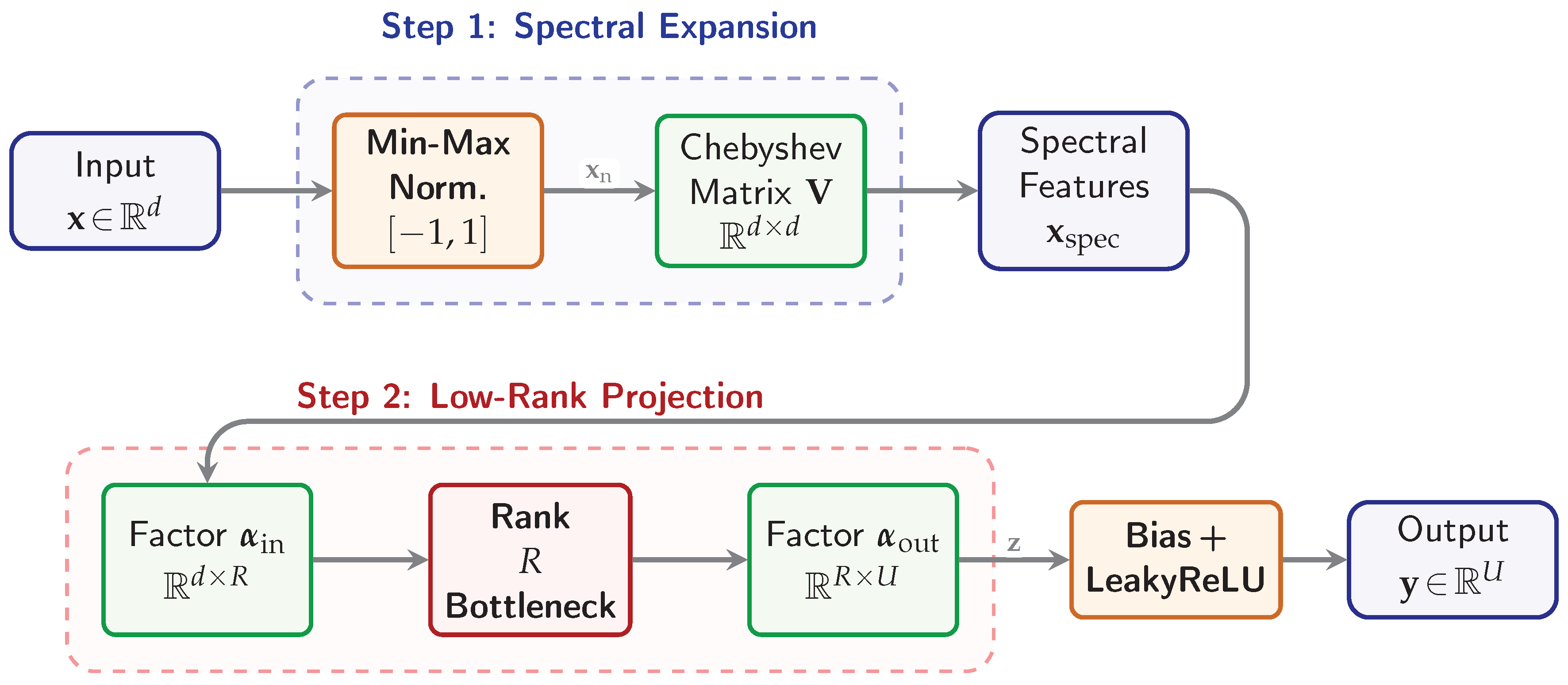
Figure 3.
STEP-3D workflow: Input volume is normalized and lifted via Chebyshev basis matrices , followed by a low-rank tensor projection through bottleneck factors .
Figure 3.
STEP-3D workflow: Input volume is normalized and lifted via Chebyshev basis matrices , followed by a low-rank tensor projection through bottleneck factors .
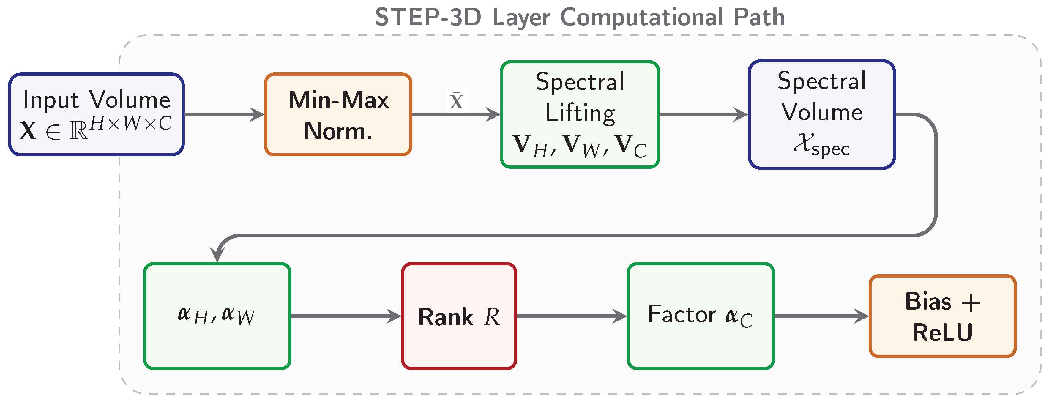
Figure 4.
Workflow of the STEP-Embedding layer. Token IDs are projected into an R-dimensional latent space, lifted via the Chebyshev basis , and processed through a non-linear rank-R bottleneck before the final expansion to .
Figure 4.
Workflow of the STEP-Embedding layer. Token IDs are projected into an R-dimensional latent space, lifted via the Chebyshev basis , and processed through a non-linear rank-R bottleneck before the final expansion to .

Table 1.
Comparison of methods for high-dimensional approximation. A check mark (✓) means that a property is fully supported or satisfied, a cross mark (×) means that it is not supported, and an approximate symbol (≈) means that it is partially or emulated supported. Here N stands for the polynomial degree in each dimension, d stands for the problem dimension, W and L stand for the network width and depth, and R stands for the tensor rank.
Table 1.
Comparison of methods for high-dimensional approximation. A check mark (✓) means that a property is fully supported or satisfied, a cross mark (×) means that it is not supported, and an approximate symbol (≈) means that it is partially or emulated supported. Here N stands for the polynomial degree in each dimension, d stands for the problem dimension, W and L stand for the network width and depth, and R stands for the tensor rank.
| Method | Scale | Curse | Theory | Tens. | NN |
|---|---|---|---|---|---|
| Poly. Exp. [25] | ✓ | ✓ | × | × | |
| Sparse Grid [26] | ≈ | ✓ | × | ≈ | |
| Dense DNN [27] | ≈ | × | × | ✓ | |
| Tensor Dec. [17,28] | × | ✓ | ✓ | × | |
| Ours (STEP) | × | ✓ | ✓ | ✓ |
Table 2.
Complexity Comparison (Function Evaluation).
| Method | Complexity (Parameters: ) |
|---|---|
| Classical Full Tensor | |
| Proposed Low-Rank Method |
Table 3.
Comparison of Classical vs STEP Approximations for Examples 1, 2, and 3.
| Function | Dim (d) | Degree (N) | Rank (R) | Classical Error | STEP Error |
|---|---|---|---|---|---|
| 1 | 2 | 10 | 2 | ||
| 1 | 2 | 10 | 4 | ||
| 2 | 3 | 10 | 3 | ||
| 2 | 3 | 15 | 4 | ||
| 3 | 4 | 10 | 2 |
Table 4.
Performance Comparison Between Traditional MLP and STEP Model on the Function Dataset (Epoch = 15).
Table 4.
Performance Comparison Between Traditional MLP and STEP Model on the Function Dataset (Epoch = 15).
| Metric | Traditional MLP | STEP | Advantage |
|---|---|---|---|
| Training Epochs | 15 | 15 | - |
| Final Val Accuracy | 0.7925 | 0.8417 | Higher Accuracy |
| Total Parameters | 149,505 | 1,316 | 99.1% Reduction |
| Inference Time | 0.0080 ms | 0.0126 ms | 1.6× Slower |
Table 5.
Performance Comparison Between Traditional MLP and STEP Model on Fashion-MNIST (1D Representation, Epoch = 11).
Table 5.
Performance Comparison Between Traditional MLP and STEP Model on Fashion-MNIST (1D Representation, Epoch = 11).
| Metric | Traditional MLP | STEP | Advantage |
|---|---|---|---|
| Training Epochs | 11 | 11 | - |
| Final Val Accuracy | 0.8771 | 0.8724 | Comparable |
| Total Parameters | 535,818 | 16,522 | 96.9% Reduction |
| Inference Time | 0.1297 ms | 0.1145 ms | 1.1× Faster |
Table 6.
Performance Comparison Between STEP and Traditional CNN (MedMNIST, Epoch 15).
| Model | Total Parameters | Accuracy | F1-score | Latency (ms) | Advantage |
|---|---|---|---|---|---|
| STEP | 34,946 | 0.8558 | 0.8493 | 0.3681 | 91.02% reduction |
| Traditional CNN | 389,250 | 0.8686 | 0.8614 | 0.7034 | Baseline |
Table 7.
Performance Comparison Between STEP and Benchmark Models (PneumoniaMNIST, Epoch 15).
| Model | Total Parameters | Accuracy | F1-score | Latency (ms) | Advantage |
|---|---|---|---|---|---|
| STEP | 42,818 | 0.8333 | 0.8225 | 0.4527 | Proposed Model |
| Traditional CNN | 389,250 | 0.8301 | 0.8167 | 0.7613 | STEP is 9.1x smaller |
| VGG16 | 14,845,378 | 0.8862 | 0.8824 | 11.1265 | STEP is 346.7x smaller |
| ResNet50 | 23,585,538 | 0.8077 | 0.7879 | 17.3907 | STEP is 550.8x smaller |
Table 8.
Performance Comparison Between STEP and Benchmark Models (Imagenette, Epoch 10).
| Model | Total Parameters | Accuracy | F1-score | Latency (ms) | Advantage vs STEP |
|---|---|---|---|---|---|
| STEP | 126,026 | 0.586 | 0.5852 | 4.7291 | Proposed Model |
| Traditional CNN | 25,787,082 | 0.262 | 0.2015 | 2.1768 | 99.51% reduction |
| VGG16 (Scratch) | 21,140,042 | 0.100 | 0.0182 | 6.5558 | 99.40% reduction |
| ResNet50 (Scratch) | 24,114,826 | 0.308 | 0.3047 | 10.4556 | 99.48% reduction |
Table 9.
Performance Comparison of Hybrid STEP Models vs Standard Deep Models on Imagenette Dataset.
Table 9.
Performance Comparison of Hybrid STEP Models vs Standard Deep Models on Imagenette Dataset.
| Model | Params | Acc | F1 | Latency (ms) | Advantage |
|---|---|---|---|---|---|
| Hybrid VGG16-STEP | 8.31M | 0.970 | 0.970 | 5.02 | Proposed Model |
| Standard VGG16 | 14.85M | 0.978 | 0.978 | 4.75 | 44.0% reduction |
| Hybrid ResNet-STEP | 1.97M | 0.958 | 0.958 | 5.23 | Proposed Model |
| Standard ResNet50 | 24.11M | 0.982 | 0.982 | 8.23 | 91.8% reduction |
Table 10.
Parameter Compression and Decoding Fidelity Across LLM Generations (Target Dim: 256). The STEP-Embedding layer maintains 100% decoding reconstruction while drastically reducing the parameter footprint.
Table 10.
Parameter Compression and Decoding Fidelity Across LLM Generations (Target Dim: 256). The STEP-Embedding layer maintains 100% decoding reconstruction while drastically reducing the parameter footprint.
| Model (Vocab Size) | Standard Params | STEP Params | Reduction | Decoding Fidelity |
|---|---|---|---|---|
| GPT-2 (50,257) | 12,865,792 | 404,424 | 96.86% | 100% |
| GPT-3 p50k_base (50,281) | 12,871,936 | 404,616 | 96.86% | 100% |
| GPT-4 cl100k_base (100,277) | 25,670,912 | 804,584 | 96.87% | 100% |
Disclaimer/Publisher’s Note: The statements, opinions and data contained in all publications are solely those of the individual author(s) and contributor(s) and not of MDPI and/or the editor(s). MDPI and/or the editor(s) disclaim responsibility for any injury to people or property resulting from any ideas, methods, instructions or products referred to in the content. |
© 2026 by the authors. Licensee MDPI, Basel, Switzerland. This article is an open access article distributed under the terms and conditions of the Creative Commons Attribution (CC BY) license (http://creativecommons.org/licenses/by/4.0/).
Copyright: This open access article is published under a Creative Commons CC BY 4.0 license, which permit the free download, distribution, and reuse, provided that the author and preprint are cited in any reuse.