

Submitted:
31 July 2026
Posted:
03 August 2026
You are already at the latest version
Abstract
Free-wake vortex-ring models are the simplest way of describing a uniformly loaded actuator disc consistently with the Euler equations, i.e. including the radial velocity that accompanies slipstream contraction or expansion. This paper examines the numerical behaviour of this model class using an independent open-source FORTRAN 90/95 implementation and a 1:1 Python replica, for the propeller case (cT = 1) and the Betz case (cT = -8/9). Three results are reported. First, the two convergence measures in common use—the residual of the wake (sheet) equations and the deviation of the power coefficient cP from momentum theory—are shown not to be equivalent: the latter has a discretisation floor and is not monotone, so it is unsuitable as a stopping criterion, and accuracy figures obtained with it are sometimes misleading. Second, the discrete Kelvin–Helmholtz saw-tooth mode is stabilised by a damping factor proportional to √z, which reaches the residual floor within a few hundred instead of 104 iterations; the remaining cP fluctuation band reflects the unresolved disc-edge region and is removed by node collocation with a spacing-proportional vortex kernel, which converges to a unique fixed point with machine-level residuals and \( c_P-(-16/27)=+4.7\times10^{-5} \). Third, the converged solutions show a bounded edge strength with fitted exponent \( a=0.00\pm0.04 \) in \( \gamma\propto s^{a} \), differing from both the \( s^{-1/2} \) spiral and the constant-\( \gamma \) proposals in the literature; we explain why single-valued, regularised sheet discretisations cannot decide this question.
Keywords:
actuator disc
; vortex ring model
; free wake
; potential flow
; momentum theory
; Betz limit
; slipstream
; edge singularity
; convergence
; Richardson extrapolation
; wind turbine aerodynamics
1. Introduction
Rotors, and wind-turbine rotors in particular, have been modelled by an axisymmetric actuator disc (AD) for more than 150 years [1,2]. In its classical form the model is evaluated by an integral momentum balance in which only the axial velocity component appears [3]. It is easily shown, however, that such a description is not consistent with the differential equations of inviscid flow, Euler’s equations,
because the radial velocity component that necessarily accompanies a contracting or expanding slipstream is discarded. Among the ways of restoring consistency without solving (1)–(2) numerically, vortex-ring (free-wake) methods [4,5] are arguably the simplest: the wake boundary is represented by a free vortex sheet whose position and strength are obtained from two physical conditions, and the velocity field follows from the Biot–Savart law in closed (elliptic-integral) form.
Starting from ye’s 1990 paper [6], this approach was developed further and applied by van Kuik and Lignarolo [7] and by Bontempo and Manna [8,9]; Conway [10] generalised the underlying analytical framework to non-uniform heavy loading. Despite this long history, three questions of practical relevance for anybody implementing such a model have, to the best of the author’s knowledge, not been answered in the open literature:
- 1.
- What do the usual convergence measures actually measure? Free-wake AD codes are commonly stopped either on a residual of the wake (sheet) equations or on the deviation of the computed power coefficient from its momentum-theory value. Are these two criteria equivalent, and does either of them certify a converged solution?
- 2.
- Is the free-wake fixed-point iteration stable, and at what price? A cylindrical vortex sheet is Kelvin–Helmholtz (KH) unstable, so any explicit update of the sheet position must be damped. Which damping keeps the scheme stable without corrupting the solution near the disc edge?
- 3.
The present paper answers these questions with the help of an independent, open-source FORTRAN 90/95 [13] implementation of the vortex-ring/vortex-cylinder model for a uniformly (constantly) loaded actuator disc, together with a 1:1 Python replica of the same algorithm that allows systematic parameter studies. The main findings are:
- The sheet residual and the momentum-theory deviation are not equivalent (Section 3). The latter possesses a discretisation floor and is not even monotone during the iteration; using it as a stopping criterion can flatter the apparent accuracy by more than an order of magnitude.
- The KH saw-tooth mode is controlled by a damping factor , which is stable for all ring numbers tested and equilibrates the edge region about two orders of magnitude faster than the damping used previously (Section 3.2).
- With midpoint collocation, retains a small residual fluctuation band that shrinks with the discretisation but not with the number of iterations; it is a property of the unresolved edge region, not an iteration deficiency (Section 3.3). Replacing midpoint collocation by node collocation with a spacing-proportional vortex kernel (Section 2.4) removes the band entirely and yields a unique fixed point with machine-level residuals.
- The converged solutions of this model class show a bounded edge strength, with a fitted exponent in — different from both proposals cited above. We show why a single-valued, midpoint- or kernel-regularised sheet discretisation is structurally unable to represent a rolled-up spiral, and why this does not affect the computed (Section 5).
The code, its Python replica, the configuration files of all cases discussed here and the GNUPLOT/Python post-processing scripts are available at https://github.com/Schaffarczyk/RingsCylinderActuatorDisk/.
2. Model and Numerical Method
2.1. Model Description
Axisymmetric coordinates are used with the velocity , non-dimensionalised with the undisturbed wind speed, , and with the disc radius, so that the disc occupies , . Its edge may carry a singularity, i.e. a point at which is not defined; this is the subject of Section 5.
The wake boundary is modelled by a piecewise linear vortex sheet which starts at and ends at , where a semi-infinite vortex cylinder (SIVC) with tangential vorticity is appended. For , N vortex rings of strength are placed with non-uniform (cosine-clustered) spacing at positions ,
so that the resolution is highest at the disc edge, where the solution varies most rapidly. This part of the approach is identical to that of [8,9].
The single physical parameter of the model is the thrust coefficient , with for the propeller case (induced velocities ) and for the turbine case; momentum theory is valid for . Several exact relations follow from momentum theory and are used below both as initial conditions and as reference values. The asymptotic radial extension of the slipstream is
giving for and for (the Betz case). The value of the total (i.e. inflow included) stream function on the slipstream far downstream is
i.e. for and for . (If only the induced part of the stream function is used, the corresponding value is ; the code works with the total stream function, Equation (6).) The model parameters are summarised in Table 1.
2.2. Induced Velocities
An accurate evaluation of the induced axial and radial velocities is the key to any arbitrarily accurate — that is, successful — implementation. The computation is split into three parts:
- 1.
- the velocities induced by the remaining vortex rings on the ring under consideration, ;
- 2.
- the self-induced velocity of the ring under consideration. Bontempo’s expressions [9] (Equations (6) and (7) therein) are used, which, remarkably, do not contain any core parameter:with the local slope of the sheet at ring m, its radial position and the distance between the two neighbouring rings. For the self-induction of vortex rings in general see, e.g., [15];
- 3.
- the velocities induced by the semi-infinite vortex cylinder at , for which the closed-form expressions of [4] (chapter 36) are used.
To avoid singular velocities on the sheet itself, all velocities are evaluated at the arithmetic midpoints of two neighbouring (singularity-carrying) sheet points. No artificial vortex core is introduced. This midpoint collocation is the classical choice; Section 2.4 discusses a structurally different alternative.
As an independent check against implementation errors, three different sets of equations for the induced velocities can be selected at run time: (i) Equations (1)–(7) of [8,9], (ii) Equation (D1) of [5], and (iii) the expressions of chapters 33 and 36 of [4]. All three agree to the accuracy of the elliptic-integral evaluation. For consistency of nomenclature, the formulation of Branlard [4] is used throughout. The complete and incomplete elliptic integrals (chapter C.4 of [4]) are evaluated with the open-source routine RFL of Carlson and Notis [16]; the implementation was verified against Mathematica to 10 significant digits.
The accuracy of the induced velocities was verified separately for the ring part () and for the cylinder part (), and against the data of van Kuik [14].
2.3. Free-Wake (Slipstream) Iteration
The shape of the slipstream is determined by the induced velocities and vice versa, through two conditions [5,8,9]:
- the sheet must be force free, implemented as with ;
- the sheet must be aligned with the flow, implemented as , Equation (6).
An initial guess for the slipstream shape reduces the number of iterations. Three options are implemented: a cylinder of radius ; the prescribed exponential shape
and a prescribed algebraic shape deduced from the axial velocity on the axis of a vortex cylinder, attributed by van Kuik [5] to Snel and Schepers,
In Equation (9), is given by Equation (5) while the decay parameter a (not to be confused with the axial induction factor) has to be estimated, . Figure 1 shows a two-parameter fit of the slipstream data of van Kuik [14], who normalises with ; the fit gives , (as it should) and .
Several update schemes for the sheet position have been implemented, selected by the parameter iter-sc:
Schemes 7 and 8 are the recommended ones; among the older schemes, No. 3 was preferred. All schemes may be under-relaxed, with for scheme 1, for scheme 2, for scheme 3 and for schemes 7 and 8, where acts as the prefactor of .
The iteration is terminated when (i) the number of iterations exceeds maxiter, (ii) the sheet residual satisfies , or (iii) (schemes 7 and 8) has stopped moving, over the last 100 iterations (Cauchy criterion). In earlier versions of the code the iteration was stopped when fell below a prescribed tolerance. As shown in Section 3, is not a valid iteration criterion.
2.4. Node Collocation with a Spacing-Proportional Vortex Kernel
The analysis of Section 3 and Section 5 identifies a structural conflict of the midpoint-collocation scheme: stability requires a position-dependent damping, the edge region remains under-determined, and retains a fluctuation band. A fourth version of the code therefore changes the discretisation itself, following van Kuik and Lignarolo [7] (Appendices A and B):
- 1.
- N vortex rings with circulations are collocated at the nodes ; ring 1 is pinned at the disc edge and exempted from the boundary conditions, in line with the discussion of the leading edge in [7] (Section 4.3 therein).
- 2.
- A vortex kernel regularises all evaluations at distances using smoothed (Marshall-type) expressions. Deviating from the fixed of [7], the kernel radius is taken proportional to the local spacing, with , which matches the analytic contribution of the local sheet strip. A fixed biases by as soon as , i.e. as soon as the spacing varies appreciably along the sheet, as it does with the clustering of Equations (3)–(4).
- 3.
-
The update is single-phase with uniform damping ,The kernel removes the saw-tooth mode (Section 3.2), so no z-dependent damping is needed. The normal-velocity (“fine-tuning”) phase of [7] (Appendix B.3) was tested and found to be neither stable nor necessary in this implementation: after the -phase, at the edge and on the sheet; it is retained only as a diagnostic (see Section 5.4).
2.5. Implementation Notes
The code is written in FORTRAN 90/95 [13] and deliberately kept simple: a minimal set of language features is used and no algorithmic “tricks” are applied, so that the source remains readable and maintainable. It consists of three files only: mem.f (global variables), VortexCode.f (the slipstream iteration loop) and SubA.f (the function library, including the elliptic integrals). Compilation uses GNU Fortran [17] with the mandatory options -fno-automatic (local variables in subroutines and functions) and -fdefault-real-8 (64-bit reals, –16 decimal digits). The latter must be applied to all source files including mem.f; otherwise the global arrays of the module remain 32-bit while the rest of the code works in double precision — an error that is easily overlooked and that limits the attainable residual to .
The power coefficient is obtained from the axial velocity at the disc following Equations (15)–(20) of [9]. The radial integration of from to uses Simpson’s rule; since this is second-order accurate, at least points are required for an accuracy of , and 3000 points are used throughout. As expected for a scheme in which every ring interacts with every other ring, the CPU time scales as (Figure 2).
All results reported below were, in addition, reproduced with a 1:1 Python replica of the code (numpy/scipy, identical Carlson elliptic integrals), which made the systematic parameter studies of Section 3 (, up to iterations) practicable.
3. Convergence Measures, Stability and the Power Coefficient
A numerical scheme deserves to be called meaningful only if it satisfies the elementary requirement
Whether a given free-wake code satisfies Equation (13) depends on which quantity “the result” refers to. This section shows that the two quantities commonly monitored behave very differently in this respect.
3.1. What the Two Convergence Measures Measure
The code monitors
These measure two fundamentally different things. is the residual of the discrete system: it can, in principle, be driven to zero by iteration alone. is the distance between the discrete solution and the continuum momentum-theory limit. Even at the exact discrete fixed point (), retains a discretisation floor made up of (i) a contribution from the ring discretisation (Table 2), (ii) a truncation error from the finite , and (iii) the contribution of the disc-edge region, which the panels cannot resolve (Section 5). Consequently neither implies nor can imply .
Three further mechanisms decouple the two measures:
- 1.
- The -weighting makes blind at the disc edge. With the cosine clustering of Equations (3)–(4), at the first ring — precisely where is largest (edge singularity) and where is most sensitive, because the weight of the power integration concentrates near . The code therefore also reports the unweighted .
- 2.
- A damping factor freezes the edge. The relaxation factor of scheme 3 vanishes at the disc, so the equilibration time of the first ring is iterations for , : reaches its floor after iterations while keeps creeping for thousands of iterations. A reference run over iterations never reached a fixed point; wandered by around at .
- 3.
- is not monotone. During this creep crosses . Values as small as occur at these zero crossings without indicating convergence at all.
Item 3 has a direct practical consequence: accuracy tables obtained by stopping the iteration on — such as Table 2, which is representative of what is found in the literature — must be read with care, since they may report the position of a zero crossing rather than a converged result.
Two implementation errors were found and corrected in the course of this analysis and are reported here because they are easy to reproduce in any comparable code: the segment length entering Equation (14) was taken from a stale variable, which made about 50 times too large, and the under-relaxation factor was applied twice, giving an effective relaxation .
3.2. Stability: The Saw-Tooth (Kelvin–Helmholtz) Mode
A cylindrical vortex sheet is KH unstable; the discrete manifestation is a saw-tooth mode on the grid scale. Systematic tests with the Python replica () gave the following picture:
- undamped Newton steps, Equation (11) with : the saw-tooth amplitude grows from to and diverges;
- constant damping: marginally stable at for and unstable for larger ; the threshold decreases with N;
- (scheme 3): stable, but the edge is frozen (see Section 3.1);
- (scheme 7): stable for and , with an edge equilibration about 100 times faster than scheme 3.
Purely local alternatives — per-station Newton iterations with a geometry-consistent finite-difference Jacobian, Gauss–Seidel sweeps, and naive streamline tracing — were also tested. They either diverge or converge to a shifted fixed point: the ring-to-ring coupling near the edge is too strong for any purely local update. This is a genuine property of the problem, not of a particular implementation, and explains why free-wake AD codes need global (or strongly damped) updates.
3.3. The Band and Its Reduction by Richardson Extrapolation
With scheme 7, drops to within iterations (, ) and then oscillates slowly around ; with the Anderson-accelerated scheme 8, reaches its floor three to four times faster still. The remaining oscillation band of , for , , is not an iteration deficiency: at the discrete equations leave the unresolved edge region — and with it — undetermined within this band. Different (all stable) update schemes converge to slightly different pseudo-solutions inside the same band. The band shrinks with increasing N and , but not with more iterations.
The code therefore reports, in addition to the last iterate, an exponentially weighted moving average of (time constant iterations) and the fluctuation band over the last 100 iterations. We recommend quoting as “average ± band” and reducing the band by an N-study with Richardson extrapolation.
Table 3 and Figure 3 show such a study for the Betz case (, exact momentum-theory value ) computed with scheme 7 at and 1100–1200 iterations per run. All extrapolation variants land at , i.e. within of . The observed convergence order is — edge-dominated, and clearly not the smooth of the ring discretisation away from the edge. The recommended citation for this protocol is .
A complementary study at fixed with , 100 and 200 gave the perhaps counter-intuitive result that a larger degrades the result: the bands grow from to and , and the means move away from . The reason is that at fixed N all cell sizes scale — the first (edge) cell even — so the loss of resolution outweighs the smaller truncation error of the cylinder, which is already subdominant at . The practical rule is therefore: use and invest the available effort in N; a double extrapolation in is unnecessary.
3.4. Node Collocation: A Unique Fixed Point
The node-collocation discretisation of Section 2.4 changes this picture qualitatively. Table 4 lists the converged results for the Betz case: the residual reaches machine level (), there is no band and no drift, i.e. the iteration converges to a unique fixed point. The error in saturates between and : the fixed points converge (Aitken limit) to , leaving an N-independent model bias of with respect to momentum theory, while the pre-saturation discretisation error decays with an observed order (Figure 4). Already at the error is , i.e. better than the midpoint scheme at .
Separating the origin of the remaining bias — truncation of the vortex tube at versus the kernel model at the tube junction and at the edge — requires runs with ; at fixed N, enlarging degrades the result because all cells coarsen, the same resolution/truncation confounding as in the -study above. In contrast to midpoint collocation, the remaining error is a smooth, pure discretisation error without band or drift, so that Richardson extrapolation is clean (Figure 4). The edge singularity itself remains kernel-smoothed; resolving the conjectured zone (Section 5) would still require an analytic edge cell or a multivalued sheet parametrisation.
4. Results for the Two Reference Cases
4.1. Propeller,
The propeller case with is only moderately non-linear: the slipstream contracts to , i.e. to about 0.93 of the disc radius, and , to be compared with the linear approximation of [18] (Equation (9.107) therein). Figure 5, Figure 6 and Figure 7 compare the computed axial velocity and vortex strength along the slipstream, and the streamline pattern, with the data of van Kuik [14]. The agreement is good over the whole range except for the immediate vicinity of the disc edge, , where the two codes deviate — exactly the region discussed in Section 5. The computed edge streamline coincides with from Equation (6), which is an independent check of the converged solution.
4.2. Betz Turbine,
For the Betz case the slipstream expands to and . Figure 8, Figure 9, Figure 10 and Figure 11 show the axial and radial induced velocities, the vortex strength and the streamline pattern. Both and tend to finite values as in these regularised solutions — a point taken up in Section 5. The converged power coefficient is (Section 3.3) with midpoint collocation and with node collocation at (Section 3.4), against the momentum-theory value .
5. The Disc-Edge Singularity
Along a force-free vortex sheet, is constant. Van Kuik [5,11] proposes that at the disc edge the wake boundary rolls up into a self-similar (Prandtl/Kaden-type) spiral whose unrolled strength diverges as
with s the arc length measured from the edge. Is Equation (16) an established result or a hypothesis? A review of the literature together with the numerical evidence of the present model gives the following picture.
5.1. What Is Established
(a) The linear (frozen-wake) model is singular at the rim. For a semi-infinite vortex cylinder of constant strength, the induced velocity field is singular at the rim: diverges logarithmically and . This is analytic — it is visible in the very Branlard expressions [4] used in this code — and Chattot [12] derives from the Biot–Savart law that the linearised slip line behaves as near the edge.
(b) The non-linear force-free problem is singular at the leading edge of the sheet. All potential-flow computations that let adjust to the force-free condition find the sheet strength growing (resolution-limited) towards the leading edge. Van Kuik [19] states that “in all flow cases the distributions have a singularity at the leading edge”, with a load-dependent strength; see also [7]. The qualitative statement “the disc edge is singular” is therefore established.
5.2. The Spiral: Strongly Supported, Not Proven
The analytical basis of Equation (16) is the local non-linear analysis of Schmidt and Sparenberg [20] for a large constant normal load. Van Kuik revisited the edge in [11] and constructed the flow induced by, and a steady solution for, Prandtl’s self-similar vortex-sheet spirals [21,22]. Equation (16) is exactly the Kaden roll-up law, which is rigorously established for the unsteady two-dimensional similarity problem (see, e.g., [15]). Independent support comes from Spalart [23], who concludes — explicitly labelling it a conjecture — that “the cross-section of the vortex sheet probably begins with a spiral”, supported by a viscous numerical solution. In contrast, Chattot [12] obtains, from a linearised analysis with a prescribed constant sheet strength, logarithmic velocity singularities and a bounded ; the disagreement is traceable to that assumption, since it is precisely the force-free coupling that drives where . No free-wake computation has resolved the spiral, and no experiment resolves the exponent. Thus the existence of the singularity is established, whereas the specific form (16) is a well-founded, independently supported, but unproven hypothesis.
5.3. Numerical Evidence from the Present Model
The converged solutions of the present model show a bounded edge strength. A log–log fit over the first rings of converged double-precision solutions (scheme 7) gives the exponents of Table 5: over two decades in s, with and, at matched s, N-independent values. This is consistent with the logarithmic decrease seen in Figure 10.
This result does not contradict the spiral picture. A discretisation of the present class is structurally unable to represent it, for three independent reasons:
- 1.
- the single-valued parametrisation of the sheet excludes any multivalued (rolled-up) geometry;
- 2.
- the self-induction term, Equations (7)–(8) (or the vortex kernel of Section 2.4), regularises the Biot–Savart kernel at the panel scale ;
- 3.
- the force-free update evaluated with this regularised velocity keeps bounded, because cannot reach zero.
The code therefore converges to the regularised solution of the no-roll-up problem, which is why the present findings differ from van Kuik’s and from Chattot’s constant- picture. Practically, the singularity is integrable (), so converges unaffected; its footprint in the computation is the saturation of at the first ring(s) and the band of Section 3.3. Any attempt to settle the exponent numerically will require either an analytic edge element or a multivalued sheet parametrisation — neither of which is contained in any of the free-wake AD codes known to the author.
5.4. A Note on the “Fine-Tuning” of van Kuik and Lignarolo
The convergence scheme of [7] (Appendix B.3) switches, after convergence of the -condition with damping 0.05, to the condition , applied as with (“fine tuning”). Transferring this second phase to a midpoint-collocation code fails structurally: after -convergence, at the first rings is — 0.9 at the first ring — which is a discretisation artefact of midpoint collocation and not a usable residual; stepping on it destroys the solution for either sign of the update. In the node-collocation discretisation of Section 2.4 the artefact disappears ( at the edge), but the -phase is then unnecessary, because the -iteration already converges to machine accuracy. It is worth noting that even in [7] the fine-tuning does not resolve the edge: a 40% violation of is reported at the first ring, and the authors conclude that the boundary conditions hold for a vortex sheet but not for its leading edge.
6. Discussion
Six model and discretisation parameters were found to influence the accuracy of the computed solution: (i) the number of rings N; (ii) the axial location of the semi-infinite cylinder; (iii) the number of integration points at the disc; (iv) the model used for the self-induction; (v) the initial and converged shape of the slipstream; and (vi) the number and distribution of vortex rings close to the disc edge. This confirms van Kuik’s finding [5] that these parameters are interrelated rather than independent. Nevertheless, increasing N always increases the accuracy, whereas increasing at fixed N does not (Section 3.3).
The results suggest the following practical recommendations for free-wake actuator-disc computations:
- 1.
- Do not stop the iteration on the momentum-theory deviation. Use the sheet residual, monitor the unweighted in addition to the -weighted mean, and treat as a verification quantity, never as a convergence criterion.
- 2.
- Quote as “average ± band” when using midpoint collocation, and reduce the band by an N-study with Richardson extrapolation rather than by more iterations.
- 3.
- Use and invest the remaining computational effort in N.
- 4.
- Prefer node collocation with a spacing-proportional kernel if a unique fixed point is required, e.g. for gradient-based optimisation or for embedding the model in a larger solver. A kernel radius proportional to the local spacing is essential on clustered grids.
- 5.
- Do not expect the edge exponent from this class of model. A bounded at the edge is a property of the regularisation, not a physical result.
Returning to Equation (13): for the sheet residual, the improved iteration demonstrably satisfies the requirement, and node collocation does so with machine-level residuals. For the requirement can hold only in the combined limit (iterations , , ), because at fixed discretisation has a floor that no iteration can undercut. This distinction is elementary, but it is not usually made explicit in the actuator-disc literature, where agreement with momentum theory to a given number of digits is often presented as evidence of numerical convergence.
The limitations of the present work should be stated clearly. The model is restricted to a uniformly loaded, axisymmetric, steady, inviscid disc without swirl; the generalisation to non-uniform loading exists analytically [10] but has not been implemented here. The remaining model bias of the node-collocation scheme ( in ) has not been decomposed into its tube-truncation and kernel contributions, which would require runs with . Finally, neither discretisation resolves the edge region itself, so the results of Section 5 bound what such models can say about the singularity rather than settling the question.
7. Conclusions
An independent, open-source FORTRAN 90/95 implementation of the vortex-ring/vortex-cylinder model for a uniformly loaded actuator disc, together with a 1:1 Python replica, was used to examine the numerical behaviour of this model class for the propeller case and the Betz case . The conclusions are:
- 1.
- The sheet residual and the momentum-theory deviation measure different things. can be driven below while stagnates at a discretisation floor; is not monotone and is therefore unsuitable as a stopping criterion.
- 2.
- A damping factor (optionally with Anderson acceleration) stabilises the Kelvin–Helmholtz saw-tooth mode and reaches the residual floor within a few hundred iterations, where the previously used damping required iterations or never settled.
- 3.
- With midpoint collocation, retains a fluctuation band ( at , ) that reflects the under-determined edge region. An N-study with Richardson extrapolation gives for the Betz case, i.e. within of .
- 4.
- Node collocation with a spacing-proportional vortex kernel and a pinned first ring converges with uniform damping to a unique fixed point (residuals , no band, no drift) and reaches , a residual model bias that is independent of N.
- 5.
- The converged solutions exhibit a bounded edge strength with fitted exponent , differing from both the spiral and the constant- picture. This is the expected behaviour of a single-valued, regularised sheet discretisation and does not decide between the two proposals; the existence of the edge singularity is established, its specific form remains an open question.
Future work should address the decomposition of the remaining model bias, the extension to non-uniformly loaded discs, and — for the edge question — an analytic or multivalued edge element capable of representing a rolled-up sheet.
Author Contributions
The author confirms sole responsibility for conceptualisation, methodology, software, validation, formal analysis, investigation, writing—original draft preparation and writing—review and editing.
Funding
This research received no external funding.
Data Availability Statement
The FORTRAN source code, its Python replica, the configuration files of all cases discussed in this paper and the post-processing scripts are openly available at https://github.com/Schaffarczyk/RingsCylinderActuatorDisk/. The reference data of [14] are available from their author.
Acknowledgments
The author would like to thank Gijs van Kuik for providing his reference data ( and ) and Emmanuel Branlard for helpful discussions.
Conflicts of Interest
The author declares no conflicts of interest.
Abbreviations
| AD | actuator disc |
| EWMA | exponentially weighted moving average |
| KH | Kelvin–Helmholtz |
| SIVC | semi-infinite vortex cylinder |
References
- van Kuik, G.; Sørensen, J.; Okulov, V. Rotor theories by Professor Joukowsky: Momentum theories. Prog. Aerosp. Sci. 2015, 73, 1–18. [Google Scholar] [CrossRef]
- Schaffarczyk, A. Introduction to Wind Turbine Aerodynamics, 3rd ed.; Springer: Berlin/Heidelberg, Germany, 2024. [Google Scholar]
- Sørensen, J. General Momentum Theory for Horizontal Axis Wind Turbines; Springer International Publishing: Cham, Switzerland, 2016. [Google Scholar]
- Branlard, E. Wind Turbine Aerodynamics and Vorticity-Based Methods; Springer: Cham, Switzerland, 2017. [Google Scholar]
- van Kuik, G. The Fluid Dynamic Basis for Actuator Disc and Rotor Theories, revised 2nd ed.; IOS Press: Amsterdam, The Netherlands, 2022. [Google Scholar]
- ye, S. A simple vortex model. In Proceedings of the Proceedings of the 3rd IEA Symposium on the Aerodynamics of Wind Turbines (IEA Annex XI), Harwell, ETSU, UK, 1990. [Google Scholar]
- van Kuik, G.; Lignarolo, L. Potential flow solutions for energy extracting actuator disc flows. Wind Energy 2016, 19, 1391–1406. [Google Scholar] [CrossRef]
- Bontempo, R.; Manna, M. A ring-vortex free-wake model for uniformly loaded propellers. Part I—Model description. In Proceedings of the Proceedings of the 73rd Conference of the Italian Thermal Machines Engineering Association (ATI 2018), Pisa, Italy, 12–14 September 2018, 2018; Energy Procedia; Vol. 148. [Google Scholar]
- Bontempo, R.; Manna, M. A ring-vortex free-wake model for uniformly loaded propellers. Part II—Solution procedure and analysis of the results. In Proceedings of the Proceedings of the 73rd Conference of the Italian Thermal Machines Engineering Association (ATI 2018), Pisa, Italy, 12–14 September 2018; Energy Procedia; 2018, p. Vol. 148. [Google Scholar]
- Conway, J. Exact actuator disk solutions for non-uniform heavy loading and slipstream contraction. J. Fluid Mech. 1998, 365, 235–267. [Google Scholar] [CrossRef]
- van Kuik, G. The edge singularity of an actuator disc with a constant normal load. In Proceedings of the Proceedings of the 22nd ASME Wind Energy Symposium, Reno, NV, USA, 6–9 January 2003; 2003, p. number AIAA-2003-0356. [Google Scholar] [CrossRef]
- Chattot, J.J. On the edge singularity of the actuator disk model. J. Sol. Energy Eng. 2021, 143, 014502. [Google Scholar] [CrossRef]
- Chapman, S. Fortran 90/95 for Scientists and Engineers, 2nd ed.; McGraw-Hill: New Delhi, India, 2013. [Google Scholar]
- van Kuik, G. Reference data for the uniformly loaded actuator disc, cT=1 and cT=-8/9. Private communication, 2021. [Google Scholar]
- Saffman, P. Vortex Dynamics; Cambridge University Press: Cambridge, UK, 1992. [Google Scholar]
- Carlson, B.; Notis, E. Algorithm 577: Algorithms for incomplete elliptic integrals. ACM Trans. Math. Softw. 1981, 7, 398–403. [Google Scholar] [CrossRef]
- The GCC Team. The GNU Fortran Compiler. Available online: https://gcc.gnu.org/fortran/ (accessed on 27 July 2026).
- Breslin, J.; Andersen, P. Hydrodynamics of Ship Propellers; Cambridge University Press: Cambridge, UK, 1994. [Google Scholar]
- van Kuik, G. On the velocity at wind turbine and propeller actuator discs. Wind Energy Sci. 2020, 5, 855–865. [Google Scholar] [CrossRef]
- Schmidt, G.; Sparenberg, J. On the edge singularity of an actuator disk with large constant normal load. J. Ship Res. 1977, 21, 125–131. [Google Scholar] [CrossRef]
- van Kuik, G. The flow induced by Prandtl’s self-similar vortex sheet spirals at infinite distance from the spiral kernel. Eur. J. Mech. B/Fluids 2004, 23, 607–616. [Google Scholar] [CrossRef]
- van Kuik, G. A steady solution for Prandtl’s self-similar vortex sheet spirals. Eur. J. Mech. B/Fluids 2009, 28, 296–298. [Google Scholar] [CrossRef]
- Spalart, P. On the simple actuator disk. J. Fluid Mech. 2003, 494, 399–405. [Google Scholar] [CrossRef]
Figure 1.
Two-parameter fit of the slipstream of van Kuik [14] according to with and . Abscissa: axial coordinate z (logarithmic); ordinate: slipstream radius r.
Figure 1.
Two-parameter fit of the slipstream of van Kuik [14] according to with and . Abscissa: axial coordinate z (logarithmic); ordinate: slipstream radius r.
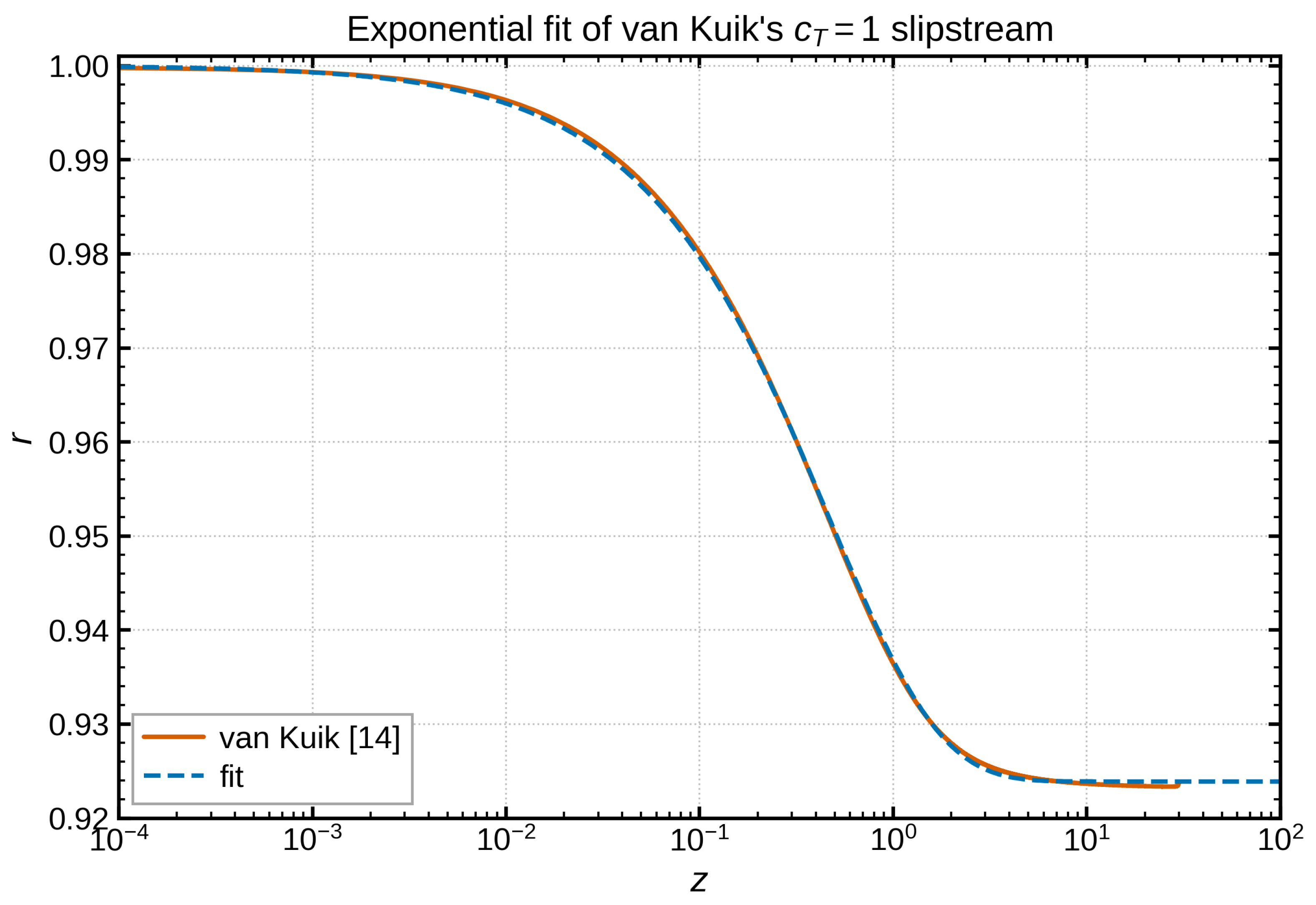
Figure 2.
Elapsed CPU time for 10 slipstream iterations as a function of the number of rings N (double logarithmic; symbols: measurement, line: fit). Hardware: Intel i3-4160 at 3.6 GHz; operating system: openSUSE Leap 42.3 Linux, kernel 4.12.14-lp151.28.44-default.
Figure 2.
Elapsed CPU time for 10 slipstream iterations as a function of the number of rings N (double logarithmic; symbols: measurement, line: fit). Hardware: Intel i3-4160 at 3.6 GHz; operating system: openSUSE Leap 42.3 Linux, kernel 4.12.14-lp151.28.44-default.
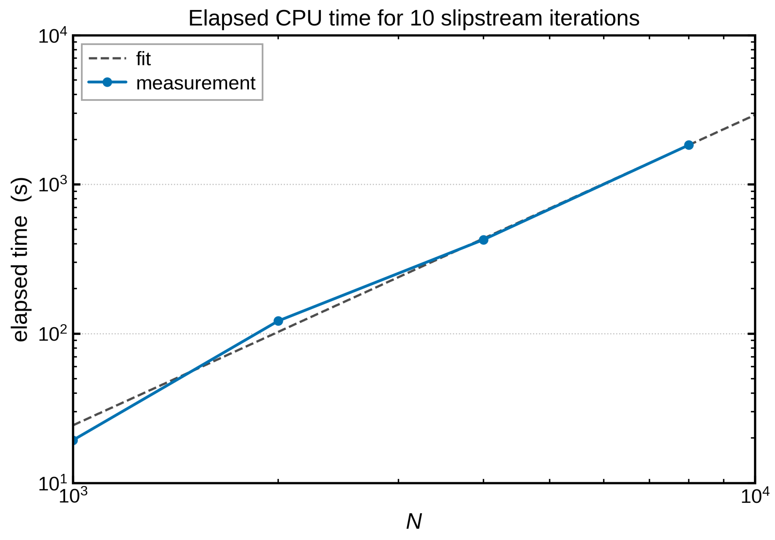
Figure 3.
Betz case, , midpoint collocation, scheme 7. (Left) Richardson extrapolation of over with the fluctuation bands as error bars; the extrapolated value is . (Right) Evolution of during the iteration for , 2000 and 4000; the dashed line is .
Figure 3.
Betz case, , midpoint collocation, scheme 7. (Left) Richardson extrapolation of over with the fluctuation bands as error bars; the extrapolated value is . (Right) Evolution of during the iteration for , 2000 and 4000; the dashed line is .
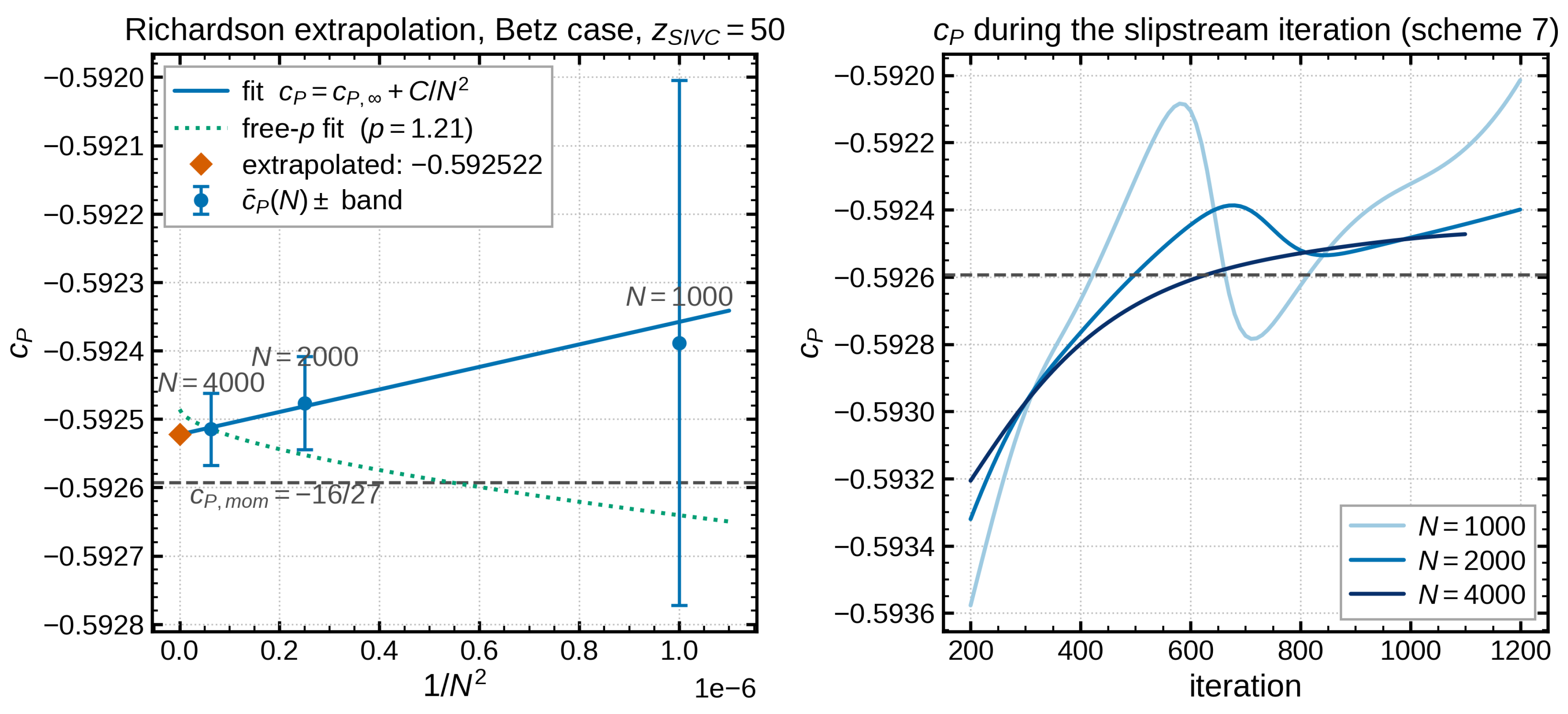
Figure 4.
Node collocation, N-study for the Betz case. (Left) Error scaling of the converged fixed points: circles, distance to ; squares, distance to the model limit . (Right) over together with the model limit and .
Figure 4.
Node collocation, N-study for the Betz case. (Left) Error scaling of the converged fixed points: circles, distance to ; squares, distance to the model limit . (Right) over together with the model limit and .
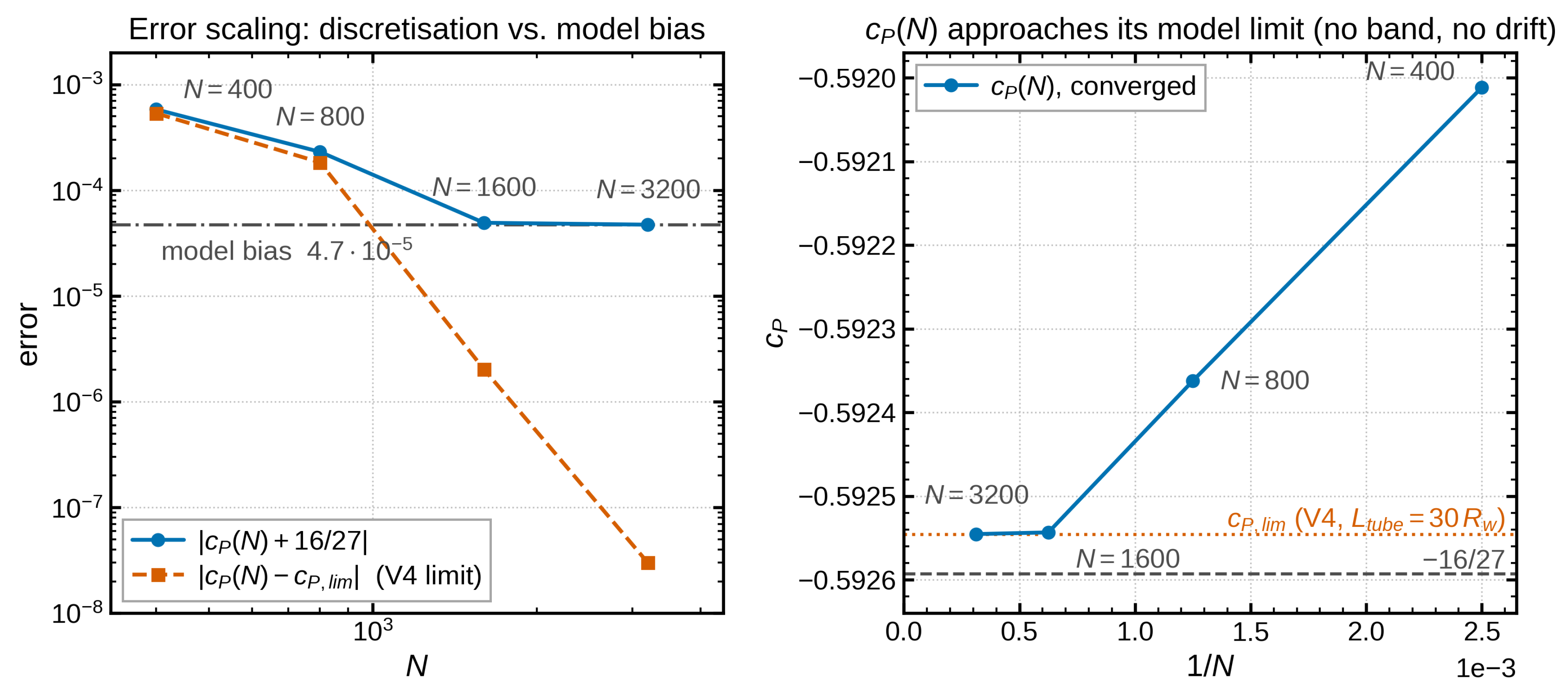
Figure 5.
Axial distribution of the induced axial velocity on the slipstream, : present code (red), data of van Kuik [14] (green), asymptotic value (black).
Figure 5.
Axial distribution of the induced axial velocity on the slipstream, : present code (red), data of van Kuik [14] (green), asymptotic value (black).
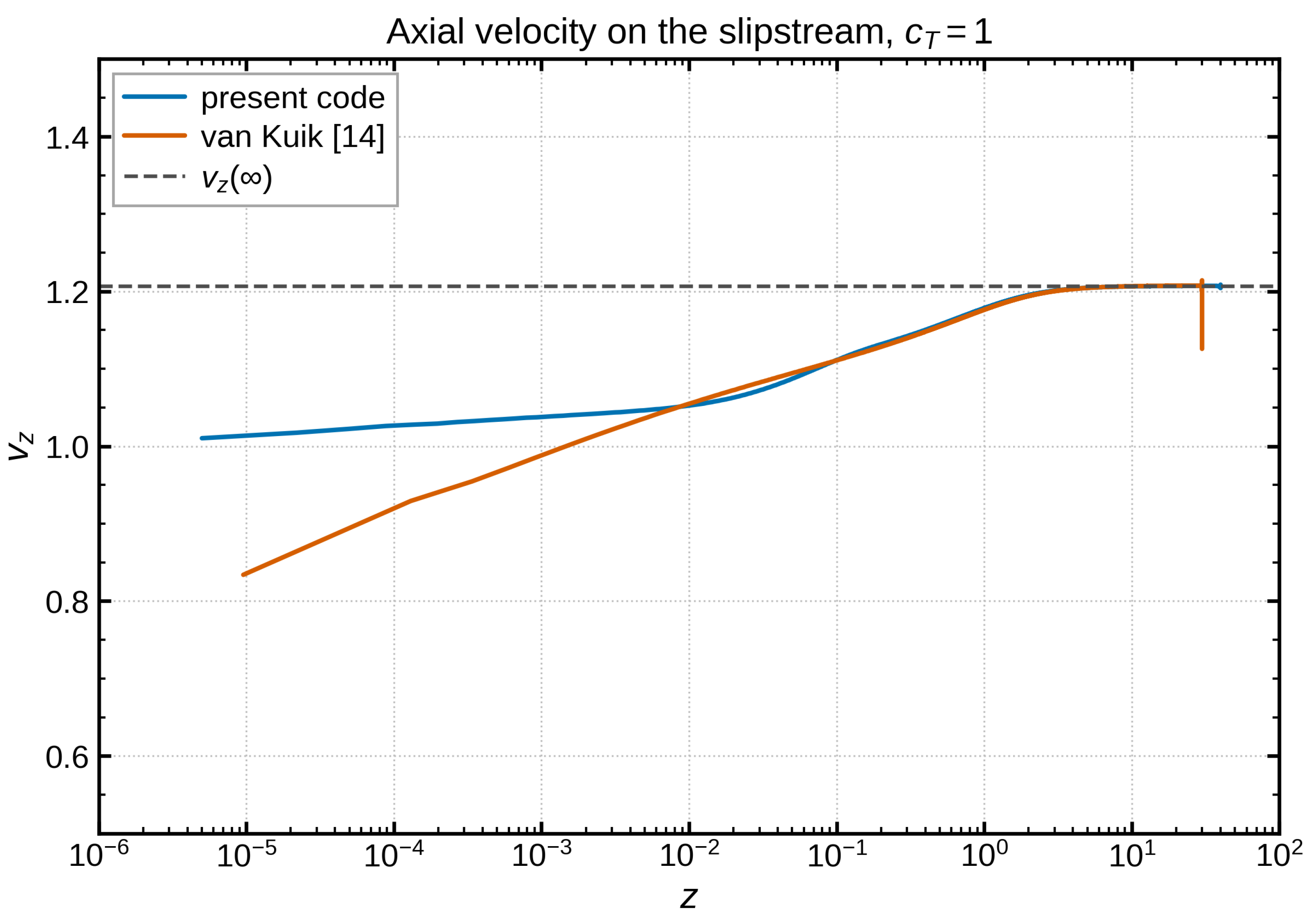
Figure 6.
Axial distribution of the vortex strength on the slipstream, : present code, data of van Kuik [14] and the momentum-theory value .
Figure 6.
Axial distribution of the vortex strength on the slipstream, : present code, data of van Kuik [14] and the momentum-theory value .
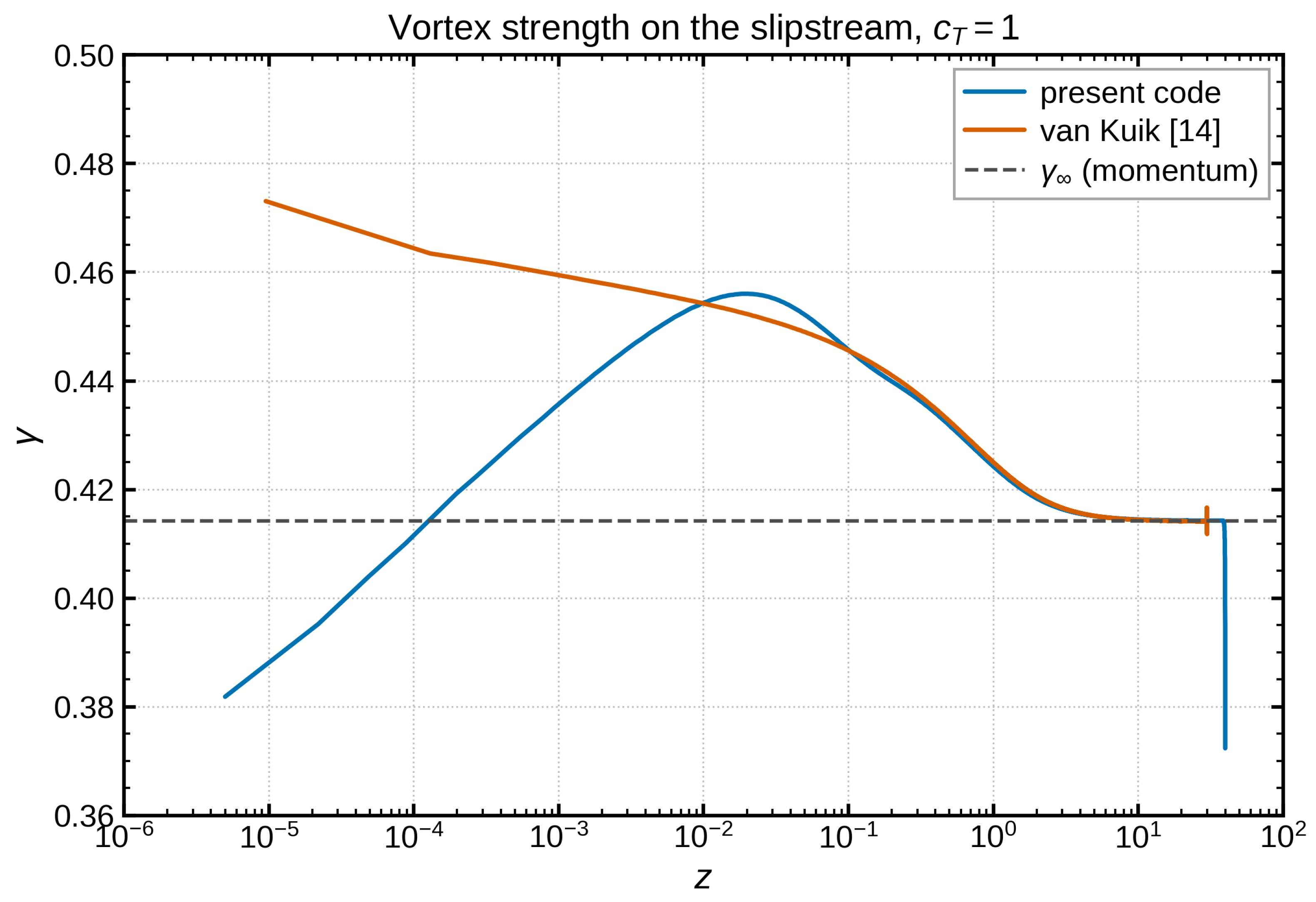
Figure 7.
Computed streamlines (lines of ) for ; the wake boundary is drawn in red. The edge streamline coincides with .
Figure 7.
Computed streamlines (lines of ) for ; the wake boundary is drawn in red. The edge streamline coincides with .
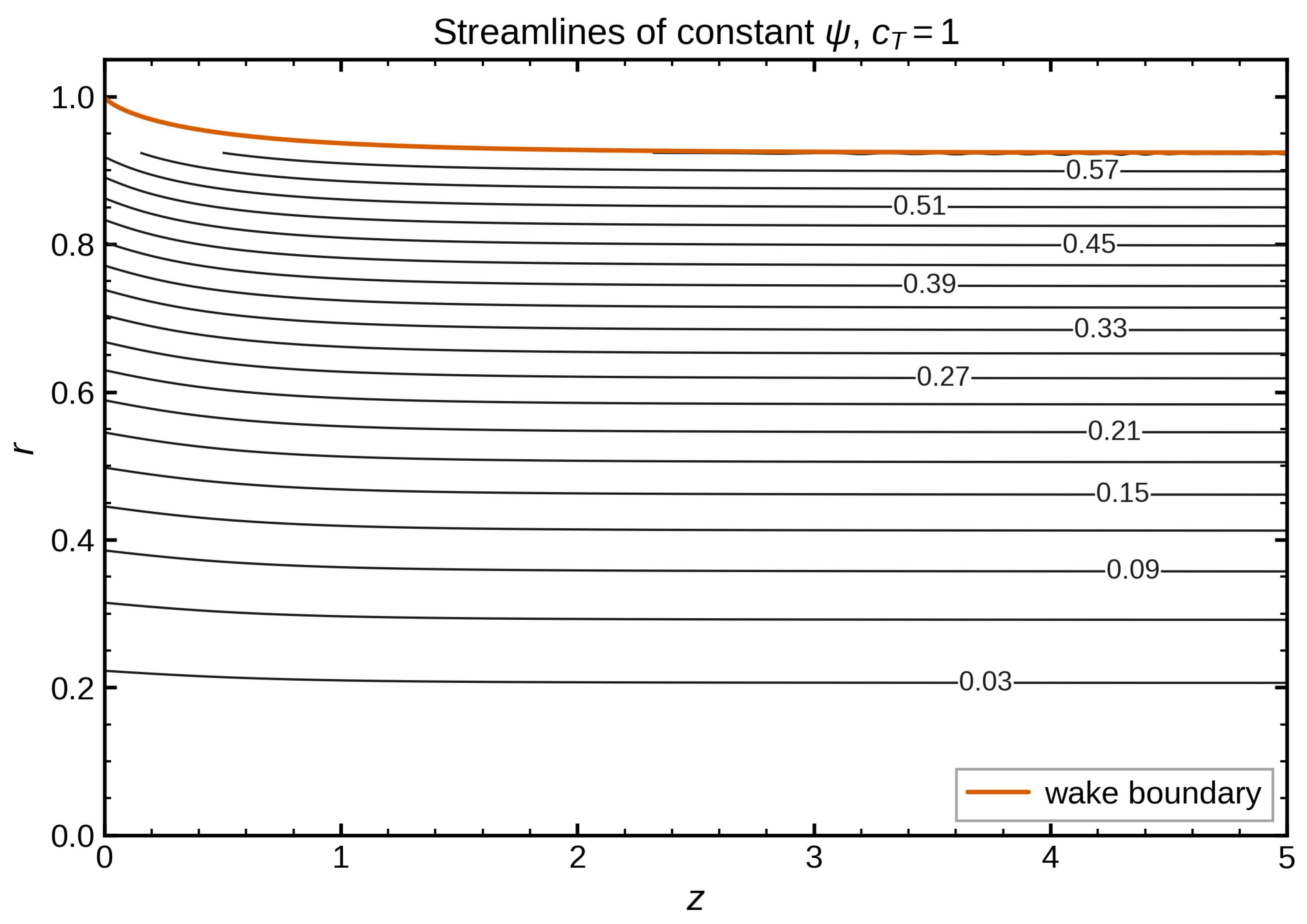
Figure 8.
Axial distribution of the induced axial velocity on the slipstream, Betz case ().
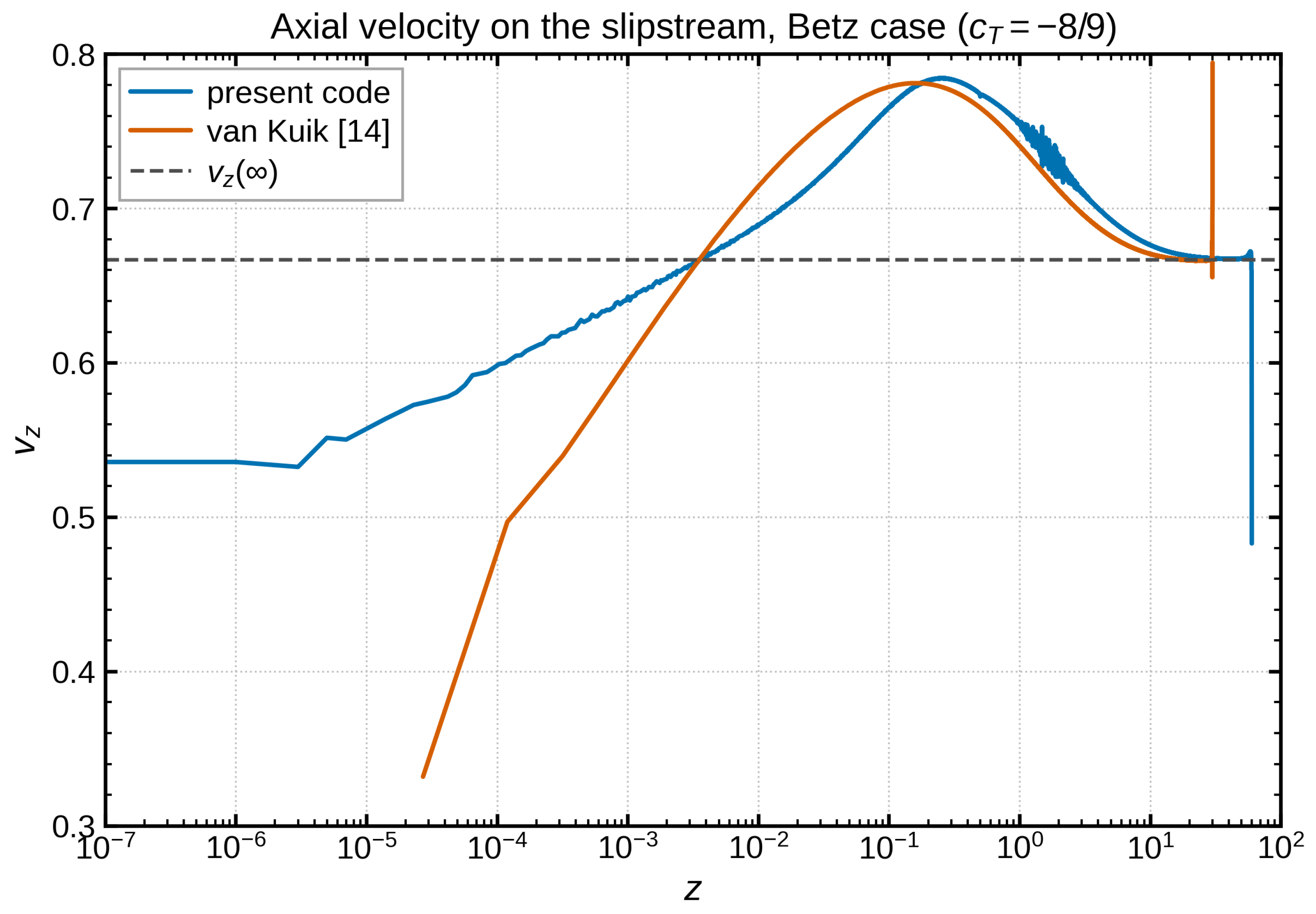
Figure 9.
Axial distribution of the induced radial velocity on the slipstream, Betz case.
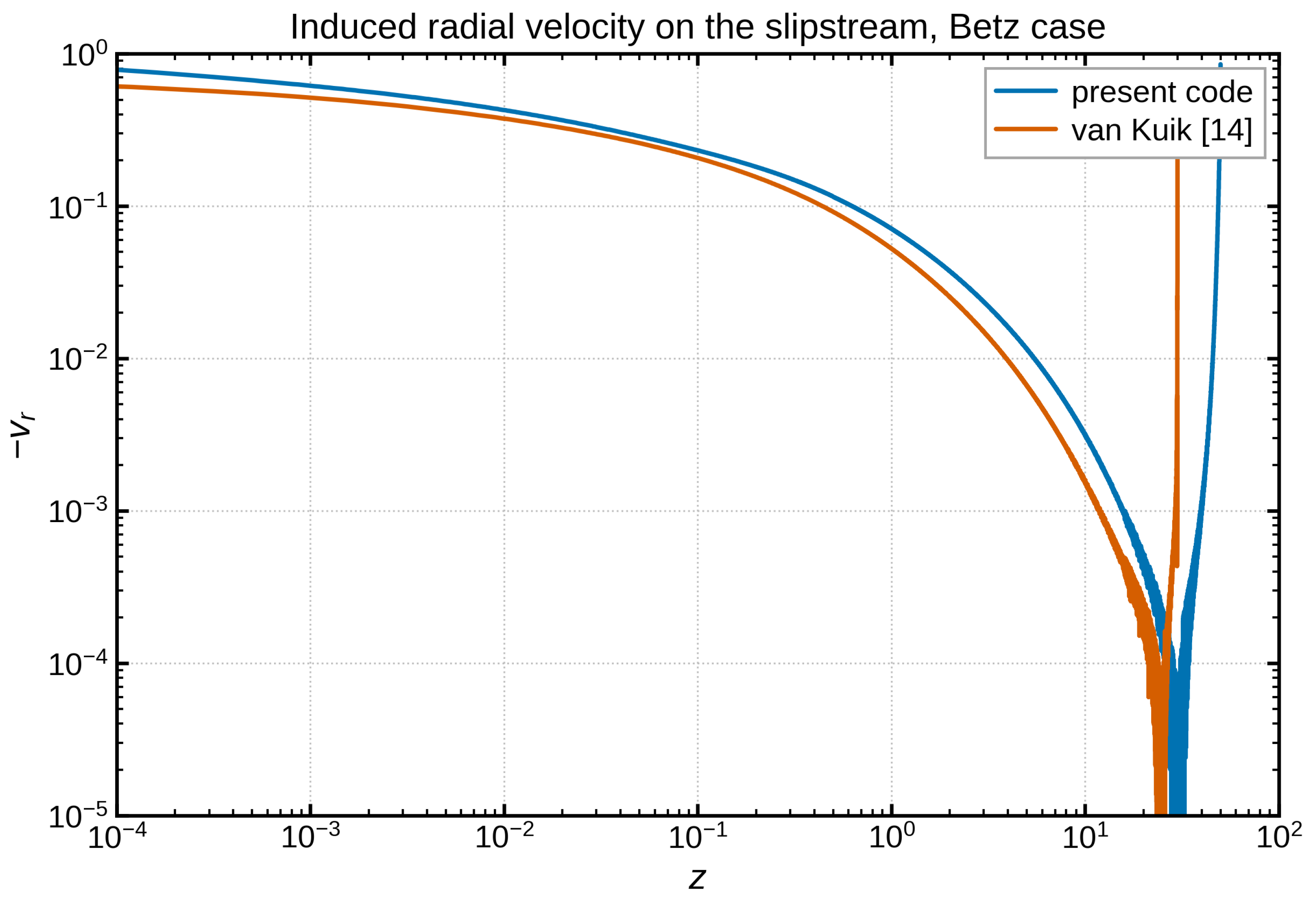
Figure 10.
Axial distribution of the vortex strength on the slipstream, Betz case. Note the logarithmic decrease towards the disc edge (small z), which corresponds to the fitted exponent of Table 5.
Figure 10.
Axial distribution of the vortex strength on the slipstream, Betz case. Note the logarithmic decrease towards the disc edge (small z), which corresponds to the fitted exponent of Table 5.
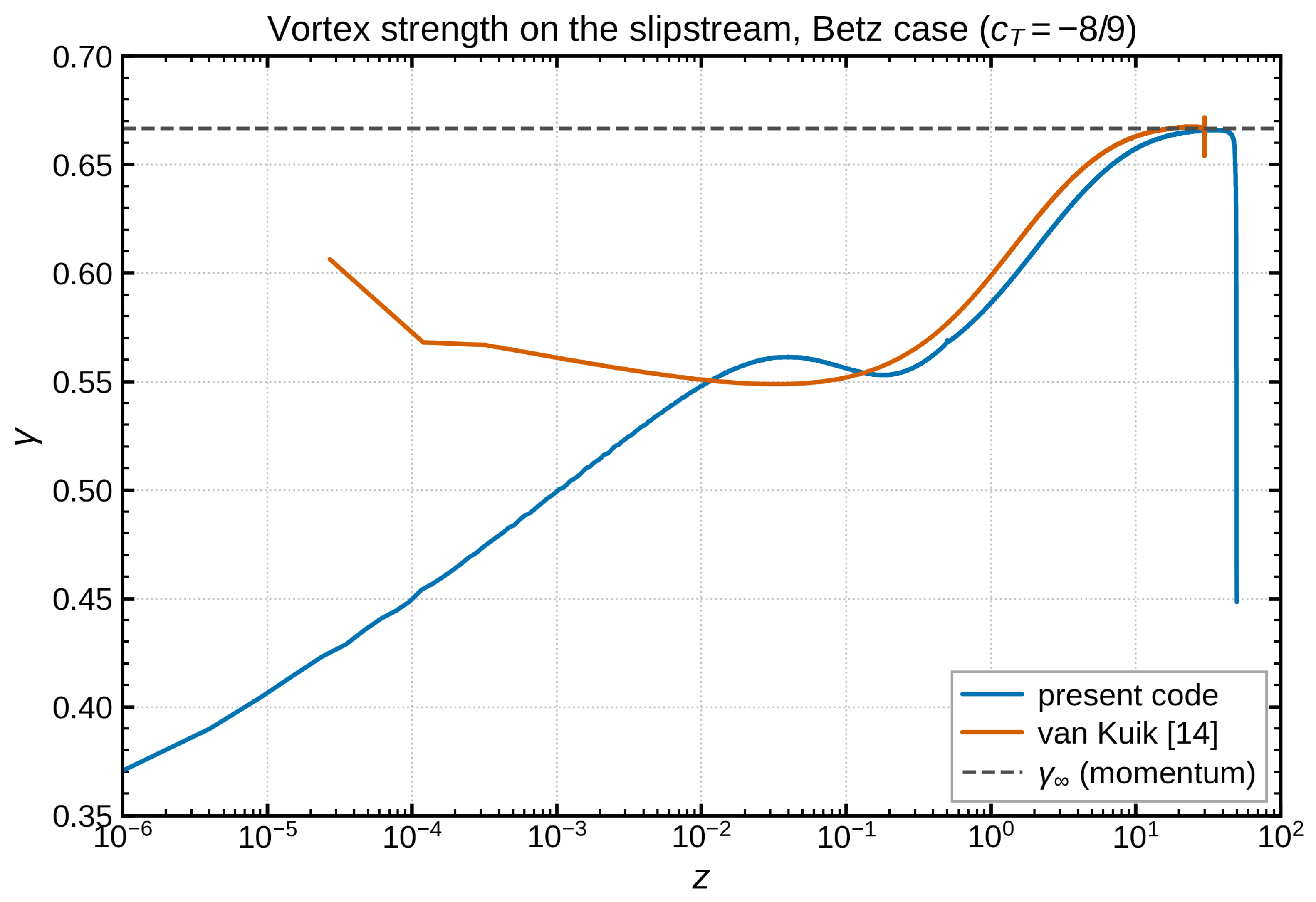
Figure 11.
Computed streamlines for the Betz case, ; red: slipstream, .
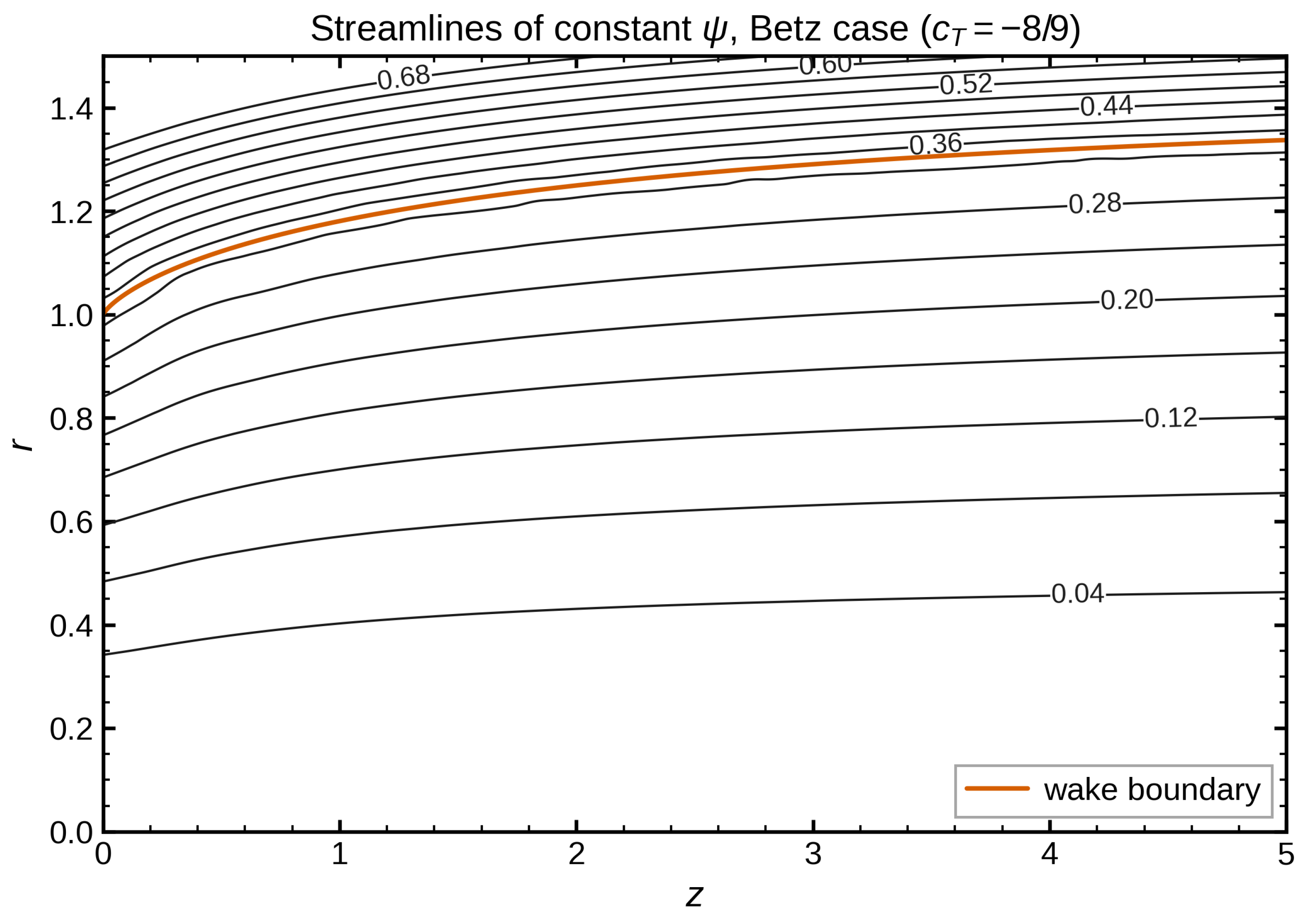

Table 1.
Major and minor parameters of the model. The names are those of the configuration file inpa.dat of the code.
Table 1.
Major and minor parameters of the model. The names are those of the configuration file inpa.dat of the code.
| Name | Meaning |
|---|---|
| major | |
| thrust coefficient | |
| restart | LOGICAL; if .true. the code restarts from an existing sls.DAT |
| N | number of vortex rings |
| ZSIVC | axial location of the semi-infinite vortex cylinder |
| minor | |
| selfind | (0,1), self-induction off/on |
| update | (0,1), default , debugging only |
| maxiter | maximum number of slipstream iterations ( used) |
| under | under-relaxation parameter, see Section 2.3 |
| epsSL | stop tolerance for the sheet residual |
| wakety | initial wake shape: 1 = exponential, Equation (9); 2 = fit of the data of [14]; 3 = algebraic, Equation (10) |
| wake-a | decay parameter a for wakety |
| iter-sc | update scheme: 3 = -condition; 7 = with -damping; 8 = 7 + Anderson acceleration; V4 = node collocation, Section 2.4 |
Table 2.
Error in as a function of the number of rings, obtained with the midpoint scheme and the iteration stopped at (). See Section 3.1 for a detailed discussion.
Table 2.
Error in as a function of the number of rings, obtained with the midpoint scheme and the iteration stopped at (). See Section 3.1 for a detailed discussion.
| Number of Rings N | Error in |
|---|---|
| 4000 | |
| 8000 | |
| 16000 |
Table 3.
N-study for the Betz case, , midpoint collocation with scheme 7. is the exponentially weighted moving average, the band is over the last 100 iterations.
Table 3.
N-study for the Betz case, , midpoint collocation with scheme 7. is the exponentially weighted moving average, the band is over the last 100 iterations.
| N | Band ± | ||
|---|---|---|---|
| 1000 | |||
| 2000 | |||
| 4000 |
Table 4.
Node collocation with a spacing-proportional kernel (Section 2.4), Betz case: the iteration converges to a unique fixed point — residuals at machine level, no band, no drift.
Table 4.
Node collocation with a spacing-proportional kernel (Section 2.4), Betz case: the iteration converges to a unique fixed point — residuals at machine level, no band, no drift.
| N | |||
|---|---|---|---|
| 400 | |||
| 800 | |||
| 1600 | |||
| 3200 |
Table 5.
Fitted edge exponents a of (Betz case, , scheme 7, converged solutions).
| Fit Window (Rings) | s-Range | a () | a () |
|---|---|---|---|
| 2–20 | |||
| 3–40 | |||
| 5–80 |
Disclaimer/Publisher’s Note: The statements, opinions and data contained in all publications are solely those of the individual author(s) and contributor(s) and not of MDPI and/or the editor(s). MDPI and/or the editor(s) disclaim responsibility for any injury to people or property resulting from any ideas, methods, instructions or products referred to in the content. |
© 2026 by the authors. Licensee MDPI, Basel, Switzerland. This article is an open access article distributed under the terms and conditions of the Creative Commons Attribution (CC BY) license (http://creativecommons.org/licenses/by/4.0/).
Copyright: This open access article is published under a Creative Commons CC BY 4.0 license, which permit the free download, distribution, and reuse, provided that the author and preprint are cited in any reuse.


