

Submitted:
03 August 2026
Posted:
03 August 2026
You are already at the latest version
Abstract
Subauroral geospace is a dynamic region. Its various features include Subauroral Polarization Streams (SAPS), hot and cold zones, and storm enhanced densities (SED). Previous studies covered the nightside leaving the dayside largely unexplored and poorly understood. This study investigates the dayside’s prenoon and midday sectors based on multi-satellite multipoint observations. As shown, dayside SAPS development was set off by solar-wind flow pressure increases compressing the dayside magnetosphere in the equatorial plane and triggering earthward-directed hot plasma surges or particle injections both in the Alfvenic solar wind and in the solar-wind-exposed dayside magnetosphere. In the inner magnetosphere, SAPS developed in a voltage generator and appeared sometimes within the hot zone where field-aligned temperature anisotropy (T‖ > T) generated electromagnetic whistler-mode chorus waves that implicitly participated in the plasma heating and sometimes within the cold zone where the isotropic ion temperature (Ti‖ ≈ Ti) minimized and electron temperature anisotropy (Te‖ > Te) generated whistler-mode hiss waves. In the ionosphere, the prenoon/midday SAPS mapped down to the noontime SED plume base depicted by the Total Electron Content maps. SAPS development was unfolding in a prenoon eastward auroral electrojet (AEJ) scenario on the dawnside or in a midday westward AEJ scenario on the duskside.
Keywords:
solar-wind dynamic pressure
; solar-wind Alfven waves
; SAPS
; hot zone
; cold zone
1. Introduction
Subauroral Polarization Streams (SAPS) are magnetosphere-ionosphere (M-I) conjugate and are the key features of the highly dynamic subauroral geospace. SAPS-related plasma turbulence, electromagnetic wave structures, and ring current ion and radiation belt electron precipitations lead to severe subauroral space weather events degrading trans-ionospheric radio signals and therefore disrupting space-based communications and navigation systems [1,2]. In the duskside ionosphere, the SAPS channel appears as a broader (2°–5°) and less intense (1000–2000 m/s) zonal plasma flow [3] driven by the underlying poleward electric (E) field that drives the plasma westward via electrodynamic E × B drifts that streams sunward along the dusk convection cell, in concert with the underlying two-cell polar convection driven by the dawn-to-dusk convection E field [4].
SAPS development on a short time scale is explained by the novel fast-time theory [5,6] derived from non-linear mechanisms and based on extensive observational evidence. Unfolding in an inner-magnetosphere voltage generator (VGM) setting, the development of outward SAPS E field in the dusk magnetic local time (MLT) sector is an essential part of the substorm current wedge 2 loop (SCW2L) system made up of large-scale Region 1 (R1) and R2 field-aligned currents (FACs). While the M-I conjugate earthward—lower-latitude R2 currents on the duskside/dawnside are downward/upward (↓/↑) directed, the M-I conjugate tailward—higher-latitude R1 currents on the duskside/dawnside are ↑/↓ directed [7,8]. In the inner magnetosphere and at the leading duskward edge of SCW, the SCW2L system demands the closure of oppositely directed ↑R1-↓R2 FACs. This is facilitated by the outward SAPS E field via meridional partial ring currents. After mapping down to the duskside ionosphere, the resultant poleward SAPS E field facilitates the closure of↑R1 currents with ↓R2 currents (flowing into the subauroral ionosphere) via poleward directed Pedersen currents. Such duskside current closure occurs at the leading edge of westward traveling surge (WTS) [8,9,10] developed at the leading duskward (or westward) edge of the auroral bulge [5,6].
Based on the novel fast-time SAPS development theory [5,6], we demonstrated and explained first [11] the development of eastward SAPS flow on the dawnside, at the dawnward (or eastward) edge of the azimuthal spreading auroral bulge [12]. More recently, we [13] demonstrated and explained the M-I conjugate SAPS phenomenon both (1) on the duskside based on the fast-time duskside SAPS development theory [5,6] and (2) on the dawnside by translating the fast-time duskside SAPS theory to the dawnside. Our M-I conjugate dawnside SAPS observations show the inner-magnetosphere inward SAPS E field in a VGM setting and its field-line mapping down to the dawnside topside ionosphere as an equatorward SAPS E field driving the plasma eastward streaming sunward along the dawn convection cell, in concert with the underlying two-cell polar convection [13].
Since the above-described past and present SAPS investigations are focused on the dusk and dawn MLT sectors on the nightside (from 18 MLT through magnetic midnight to 6 MLT), these studies do not cover the dayside (from dawn through midday to dusk). Consequently, dayside M-I conjugate SAPS investigations focusing on the prenoon and midday MLT hours are still rare and create a knowledge gap in our understanding. In order to contribute to filling this knowledge gap and to increase our understanding of midday subauroral geospace, we conducted for the first time a detailed investigation on the prenoon and midday SAPS phenomenon.
Our main aim is to investigate inner-magnetosphere SAPS E field development and plasma environment. We focus on their characteristic features (listed below as a–c), on the 10–12 MLT sector, and on the dayside magnetic equatorial plane. These characteristic features include (a) storm enhanced densities (SED) [14] transported to the noontime cusp by the poleward SAPS E field from the dusk sector and then into the polar region by the dawn-to-dusk convection E field [15,16,17], (b) hot and cold zones appearing as localized ion temperature increases and decreases near the inner-magnetosphere plasmapause [18], and (c) electromagnetic whistler-mode waves propagating through the magnetized plasma near the equatorial plane along the magnetic field lines [19].
Significantly, we investigate prenoon (~10 MLT) and midday (11.5–12.0 MLT) SAPS E field development both (1) near the magnetic equatorial plane and (2) in a magnetosphere voltage generator (VGM) setting based on the novel fast-time duskside SAPS development theory [5,6]. Scientifically correctly, we apply the duskside SAPS theory to the midday outward SAPS E field observed on the duskside and translate the duskside SAPS theory to the dawnside, where the prenoon inward SAPS E field was observed. For triggering SAPS development in the prenoon and midday sectors, we consider the increased solar-wind dynamic pressure (Pdyn) compressing the dayside magnetosphere in the equatorial plane. This is where whistler-mode chorus waves are generated in the inner magnetosphere [20,21] and whistler-mode hiss waves are produced in the plasmasphere [22]. Furthermore, such solar-wind Pdyn increases drive intense inner-M—I interactions [23,24] via the intensifications of auroral electrojets (AEJ) and R1 FACs [25]. These intense interactions are favorable for the generation of R2 currents [26] that are essential to inner-magnetosphere SAPS E field development on the duskside [5,6] and in the prenoon and midday sectors as documented in this study.
2. Materials and Methods
In this study, we present various inner-magnetosphere prenoon/midday SAPS scenarios, depicting the inward/outward SAPS E field and associated phenomena, observed by the Time History of Events and Macroscale Interactions during Substorms (THEMIS) [27] mission’s three Earth orbiting satellites (TH-A, TH-D, and TH-E). We used prenoon and midday measurements taken during 2012, when these THEMIS satellites completed their Dawn Science Phase and their highly elliptical orbits reached ~12 RE on the dawnside. To investigate the inner-magnetosphere SAPS E field, we used E field components (EX, EZ; mV/m) measured in Geocentric Solar Magnetospheric (GSM) coordinates by the Electric Field Instrument (EFI) suite [28]. To investigate the inner-magnetosphere SAPS E field’s plasma environment, we used measurements provided by the Elastic Analyzer (ESA) suite [29,30] such as spacecraft (SC) potential (SC Pot; V), hot ion density (Ni; cm−3) and hot electron density (Ne; cm−3), electron flux measured between 2.97 keV and 6.86 keV energy levels, and ion temperature (Ti) measurements made parallel (‖, Ti‖; keV) and perpendicular (⊥, Ti⊥; keV) to the ambient magnetic field. From the On-board Moment (MOM) suite, we used electron temperature (Te) (Te‖; Te⊥; keV) and velocity (Ve||; km/s) measurements. From the Ground-Calculated Particle Moments (GMOM) suite, containing combined data from the suites of ESA and Solid State Telescope (SST) [27], we used pressure tensor measurements taken in the XX direction for ions (PiXX; keV/cm−3) and electrons (PeXX; keV/cm−3). Finally, the Search-Coil Magnetometer (SCM) [31] suite measured the fluctuations of B field components (BX, BY, BZ; nT) in the 0.1 Hz–4.0 kHz range in GSM coordinates for observing whistler-mode chorus and hiss waves.
For obtaining magnetosphere observations of dayside earthward directed plasma injections and plasma surges occurring during the prenoon and midday SAPS events, we used various data types provided by the GEOTAIL satellite orbiting the Earth with a 30 RE apogee and 9 RE perigee [32]. These data types include ion differential intensity measured at 67–1361 keV energy levels by the Energetic Particles and Ion Composition (EPIC) suite [33], ion bulk flow velocity components (ViX, ViY, ViZ; km/s) measured in solar wind in Geocentric Solar Ecliptic (GSE) coordinates by the Comprehensive Plasma Instrument/Solar Wind Analyzer (CPI/SWA) suite [34], hot plasma pressure measurements recorded by the CPI suite [34], and magnetic B field components (BX, BY, BZ; nT) measured by the Magnetic Field Instrument (MGF) suite [35] in GSM coordinates.
For investigating topside-ionosphere midday SAPS flows, we used Defense Meteorological Satellite Program (DMSP) data. Polar orbiting DMSP satellites circle the Earth at ~840 km altitude in the topside ionosphere (orbital period of ~101 min; inclination angle ~98.7°) and carry various instruments [36]. From spacecraft F16, we utilized electron density (Ne; 1/cm3) data provided by the Langmuir Probe (LP), electron and ion temperature (Te, Ti; K) data from the Retarding Potential Analyzer (RPA), cross-track horizontal (HOR; sunward-antisunward) and vertical (VER; upward-downward) ion drifts (VHOR, VVER; m/s) from the Ion Drift Meter (IDM), and magnetic vertical (Z; upward-downward) deflection component (δBZ; nT) derived from the Special Sensor Magnetometer (SSM) data [37]. Based on previous studies [38,39], we computed the vertical component of Poynting flux (S‖; mW/m2) in spacecraft-centered coordinate system, where X is upward-downward, Y is forward-backward, and Z is eastward-westward. We used the equation of S‖ = 1/μ0((VXBZ − VZBX)dBZ − (−VXBY)dBY), where μ0 is the permeability in vacuum (4π × 10−7 H/m). Here, the values of S‖ < 0 represent downward or earthward directed Poynting flux deposited into the coupled ionosphere-thermosphere (I-T) system. But for our presentation in this study, we plotted the earthward directed S|| data as positive values.
For investigating the prenoon/midday SAPS flows’ auroral and subauroral electrojet environments, we utilized the vector plots of magnetic perturbations measured in the horizontal direction. These imageries are provided by the Active Magnetosphere and Planetary Electrodynamics Response Experiments (AMPERE) [40,41].
Orbit data provided by THEMIS, GEOTAIL, and DMSP include orbit parameters in GSM coordinates, magnetic local time (MLT; Hr), L shell (RE), satellite footprints in geographic [longitude (GLON), ° E; latitude (GLAT), ° N] coordinates, geomagnetic latitude (MLAT; ° N), and solar local time (LT; Hr).
For monitoring the prevailing northern-hemisphere total electron content (TEC) variations, we used vertical TEC data computed in TEC units (TECU; 1 TECU = 1016 e−/m2) for the mean ionospheric height of 350 km. These TEC data are published by the Madrigal database as automatically processed values derived from the raw satellite data provided by the worldwide ground-based Global Navigation Satellite System (GNSS) receiver network and then averaged over 5 min (in UT) and binned in 1° latitude by 1° longitude (geographic) cells [42].
For investigating the underlying solar wind conditions, we used time-shifted Advance Composition Explorer (ACE) [43] satellite measurements collected on the dayside in solar wind. Published by the OMNI database, these ACE data are shifted in time to the nose of the bow shock [44] and include solar-wind velocity components (VX, VY, VZ; km/s) and Interplanetary Magnetic Field (IMF) components (BX, BY, BZ; nT) measured in GSE coordinates, total B field (BT; nT), solar-wind dynamic pressure (Pdyn; nPa) and Interplanetary Electric Field (IEF) EY (mV/m) component in GSM coordinate. Based on recent work [45], we computed the IEF field-line parallel (‖) component (IEF E‖; mV/m) in GSM coordinate as E‖ ≈ EYBY/((BY)2 + (BZ)2)−2.
For investigating the underlying geomagnetic conditions, we used the geomagnetic indices of SYM-H (nT) and ASY-H (nT) for observing the magnitudes of ring current and partial ring current variations, Kp for observing the intensity of geomagnetic activity, and AE (nT) for observing the strength of auroral activity, and polar cap north (PCN; mV/m) for observing the intensity of northern-hemisphere polar convection over the northern magnetic pole [46] driven by the merging E field (Em) [47]. For specifying substorm onset times, we utilized substorm list [48,49] published by SuperMAG.
3. Results
3.1. Dawnside and Duskside SAPS Scenarios
Focusing on the magnetic equatorial plane’s prenoon and midday MLT sectors, Figure 1 illustrates two sets of schematic diagrams depicting the M-I conjugate SAPS phenomenon in these MLT sectors. While the dawnside scenario is shown in Figure 1a (see also Figure 7a–c), the duskside scenario is shown in Figure 1b (see also Figure 8a).
Overall, the dayside inner-magnetosphere hot plasmasheet plasma is illustrated with hot ion (in magenta) and hot electron (in light blue) measurements made by THEMIS. In the magnetic equatorial plane, the inner-magnetosphere net SAPS E field is located near the inner-magnetosphere plasmapause (PP; dotted line in cyan).
Figure 1a shows the inner-magnetosphere inward (or earthward) prenoon SAPS E field (inward arrow in light blue), which developed on the dawnside. By mapping down to the northern-hemisphere subauroral ionosphere, near the PP, the resultant equatorward SAPS E field (equatorward arrow in light blue) drives the plasma eastward (via electrodynamic E × B drift) in the dawnside SAPS flow channel.
Figure 1b illustrates the inner-magnetosphere outward (or sunward) near midday SAPS E field (outward arrow in dark blue), which developed on the duskside. By mapping down to the northern-hemisphere subauroral ionosphere, near the PP, the resultant poleward SAPS E field (poleward arrow in dark blue) drives the plasma westward (via electrodynamic E × B drift) in the duskside SAPS flow channel.
Figure 1a,b shows that these inner-magnetosphere SAPS E fields develop in their respective magnetosphere voltage generator (VGM) settings. Charge separation forms between the hot positive plasmasheet ions (+; in light magenta) and hot negative plasmasheet electrons (−; in lighter blue) created by steep plasma density or plasma pressure gradients [6]. Accordingly, as shown in Figure 1a with dawnside plasma pressure measurements of the dawnside SAPS scenario, the hot electron pressure drop is located earthward while the hot ion pressure drop is situated sunward. Oppositely, as Figure 1b illustrates the duskside midday SAPS scenario with hot plasma density measurements, the hot ion density gradient is located earthward while the hot electron density gradient is situated sunward.
3.2. THEMIS and GEOTAIL Orbit Configurations
Our observational results illustrate four inner-magnetosphere SAPS events: one prenoon (~10 MLT) SAPS event on 22 March 2012 (Event-1) and three midday (11.5–12.0 MLT) SAPS events on 20 and 22 February and 3 March 2012 (Events 2–4).
In Figure 2, we show four sets of X versus Z and X versus Y orbit plots illustrating the orbit sections of interest completed by THEMIS close to Earth and by GEOTAIL away from Earth in these four SAPS events. During their respective travel times, the three THEMIS satellites (TH-A in orange, TH-D in red, and TH-E in light green) were traveling earthward on the dayside and close to the magnetic equatorial plane, sometimes just below (see Figure 2a) and sometimes just above (see Figure 2b-e) the magnetic equator. During the time-periods of interest, the three THEMIS satellites observed the solar-wind-exposed inner magnetosphere. GEOTAIL (marked in blue) was traveling on the dayside and thus was able to observe the solar-wind-exposed magnetosphere during the time-periods under study.
3.3. Underlying Conditions
3.3.1. Underlying Interplanetary and Geomagnetic Conditions
With four sets of line plots, Figure 3a–d illustrate the underlying solar and geophysical conditions of the four SAPS events investigated. Each line-plot set covers the SAPS event’s larger time-period including the entire previous day and the actual event day up to 16 UT. These line plots illustrate the SW, IMF and IEF variations with the ACE-measured variables of IMF BT, SW-IMF components (VX-BX; VY-BY; VZ-BZ), IEF dawn-dusk EY and north-south E|| components, and solar-wind dynamic pressure (Pdyn). Meanwhile, the underlying geomagnetic conditions are depicted by the geomagnetic indices of SYM-H and ASY-H, Kp and PCN, and AE. In each line-plot set, we marked the SAPS event observed by THEMIS (shaded interval in yellow) and its larger time-period extending from 21.0 UT through 24 UT to 5.0 UT (shaded interval in light green). Because of the close similarities shown by the four line-plot sets, we describe first the similar features and then highlight the event-specific features.
In each line-plot set, the IMF BT line plot shows an overall increase during this larger 21.0-5.0 UT time-period (shaded interval in light green). As illustrated with the closely correlated variations of the respective SW drift velocity and IMF B field components (VX-BX; VY-BY; VZ-BZ), the solar wind was highly Alfvenic [50] during the entire time-period covered. Importantly, during the SAPS event (shaded interval in yellow), the IMF BT and IEF EY and E|| components along with the solar-wind Pdyn simultaneously increased. These important signatures imply (i) the dayside magnetosphere’s solar-wind compression [23] by the increased solar-wind Pdyn, and (ii) the compression-related overall strengthening of IMF [51,52,53] by the increased IMF BT, (iii) the compression-related zonal solar convection increase [54] by the increased IEF EY, and (iv) the increased-convection-related field-aligned solar plasma acceleration [45] by the increased IEF E|| creating field-aligned temperature anisotropy (T‖ > T⊥) and intensifying chorus waves [55]. Characteristic to SAPS Event-1, the localized BT minimum (shaded interval in yellow in Figure 3a) implies favorable conditions created for whistler-mode chorus wave generation [56].
As shown by the geomagnetic indices, the underlying geographic conditions remained mostly quiet (Kp < 3 and AE < 400 nT) during these SAPS events except the second event that occurred at the end of the recovery phase of a weak (SYM-Hmin ≈ −80 nT) geomagnetic storm (see Figure 3b). Overall, ASY-H increased implying intensifying partial ring currents [57] and PCN peaked implying strengthening polar convections [46].
3.3.2. Underlying Alfvenic Solar Wind Conditions
Figure 4a shows four line-plot sets constructed with the GEOTAIL-measured variables of hot-ion-drift—magnetic-field components (VX-BX; VY-BY; VZ-BZ) covering the respected SAPS events’ larger time-periods (21.0-5.0 UT; shaded interval in light green). In each set, we marked the THEMIS-observed SAPS event (shaded interval in yellow). These time-series depict close correlations between the respective hot ion velocity and B field components measured in solar wind and thus provide observational evidence of the solar-wind-exposed dayside magnetosphere’s Alfvenic nature. During each SAPS event (shaded interval in yellow), there was a temporary ion-drift—B-field component increase. Notably, the ion drift increase was part of a series of earthward directed hot ion drift surges, which occurred when the solar-wind dynamic pressure (Pdyn) increased in the Alfvenic solar wind (observed by ACE and shown in Figure 3).
Figure 4b–d illustrate two sets of velocity versus B field scatter plots constructed based on a previously established methodology [58] with GEOTAIL and ACE data respectively. These scatter plots show the strong positive linear correlations, which are typical to Alfven waves [58], between the hot ion drift and magnetic B field components observed by GEOTAIL in the solar-wind-exposed dayside magnetosphere (shown in Figure 4b) and between the SW velocity and IMF B field components observed by ACE within the solar wind (shown in Figure 4c). While the scatter plots’ respective linear correlations indicate the Alfvenic nature of solar-wind-exposed dayside magnetosphere (observed by GEOTAIL) and solar wind (observed by ACE), their respective positive gradients imply earthward propagating Alfven waves [58]. We note here the scattered nature of 21–22 February 2012 GEOTAIL scatter plots because of the incomplete data coverage.
3.3.3. Underlying Dayside Magnetosphere Conditions
Figure 5 shows four sets of plots constructed with GEOTAIL data in order to further illustrate the underlying dayside conditions prevailing in the solar-wind-exposed magnetosphere. Each line-plot set covers the larger time-period of 21.0-5.0 UT (shaded interval in light green) of the four SAPS events (shaded interval in yellow). Commonly, these line-plot sets are constructed with the GEOTAIL-measured differential ion intensity covering the 67.3–538.8 keV range (see top panel) and hot ion velocity (see bottom panel).
Figure 5a,d show a series of earthward directed hot differential ion intensity increases (in the top panels) driven by the increased hot ion drift surges (in the bottom panels) propagating earthward. We note again that these earthward directed increases and surges were highly Alfvenic (observed by GEOTAIL; see Figure 4a–b). THEMIS observed the daytime SAPS event during one of the hot ion drift surges and when the solar-wind dynamic pressure peaked (observed by ACE). This is further illustrated in Figure 5d with the GEOTAIL-measured hot ion bulk flow speed (middle panel) and ACE-measured solar-wind Pdyn plot (bottom panel) depicting a series of simultaneous undulations. The strong similarity between the GEOTAIL and ACE line plots provides further verification and observational evidence of the ACE-observed solar-wind dynamic plasma pressure (Pdyn) undulations driving the GEOTAIL-observed earthward-directed hot ion surges. These imply that the dayside magnetosphere’s solar-wind compression enhanced the dayside plasma convection [54] that is also evidenced by the increased IEF EY and E|| components (shown in Figure 3).
In Figure 5b,c, the GEOTAIL differential ion intensity plots show a series of earthward-directed hot ion injections observed on the dayside. These dispersionless hot ion injections’ signatures appear at all the intensity levels covered [59] and are depicted in Figure 5b by the simultaneously increased differential ion intensities and in Figure 5c by two sets of particle injections. These dispersionless particle injections were driven by the underlying earthward-directed hot ion flow surges shown in the bottom panel. In Figure 5c, we show also the hot plasma pressure (in the bottom panel) showing a large increase just before the second injection. Thus, these earthward-directed hot ion injections’ solar-wind drivers were the increased solar-wind dynamic pressure pulses [54,60], as shown by the Pdyn line plot within the shaded interval (in light green) in Figure 3. All these observations of Figure 5b,c provide evidence of the earthward-directed particle injections occurring on the dayside and near the magnetic equatorial plane [59] before and during their respected midday SAPS events were observed THEMIS. Furthermore, in the solar-wind-exposed dayside plasmasheet, THEMIS observed the signatures of earthward-directed hot electron injections that are depicted by the THEMIS-measured differential electron fluxes (shown in Figure 8a,b).
Notably, in each SAPS event, the dayside earthward-directed hot plasma surges/particle injections resulted in charge separation at the midday plasmapause (as shown in Figure 8a; see details below) and resulted in dayside SAPS development in a magnetosphere voltage generator (VGM) setting.
3.3.4. Underlying Ionospheric TEC Conditions
Figure 6a–d show the northern-hemisphere map and polar plot sets constructed with GNSS TEC data for their respective four SAPS events. Each map covers the one-hour time-period, during which the SAPS event was observed by THEMIS. With the maximum TEC values of ≥25 TECU (in dark red), each TEC map shows the SED plume base where the prenoon or midday SAPS mapped down (dot symbols in colors) to ~120° E geographic longitude and ~65° N geographic latitude. For better visibility, we circled (in white) the mapped-down prenoon SAPS location. In the LT versus GLAT polar TEC plot, the high TEC values of >18 TECU (in shades of red) show (i) the SED plume base covering a larger region of local noon (12 LT), where the prenoon or midday SAPS and (ii) the convection of SED plume into the polar region at ~14–15 LT.
3.4. SAPS Events: SAPS E Fields and Their Plasma Environment Observed by THEMIS
3.4.1. SAPS Event-1: Prenoon Inward SAPS on 22 March 2012
Figure 7a–c covers the time-periods of interest on 22 March 2012, when the inner-magnetosphere prenoon SAPS channel was observed by the three THEMIS satellites on the dayside and dawnside, and near the magnetic equatorial plane (as shown by the orbit plots in Figure 2a). These line-plot sets are arranged in increasing UT SAPS detection order and are plotted in the earthward direction (from left to right). These plots depict at ~10 MLT, the prenoon SAPS observed by TH-D just before 1.5 UT (in Figure 7a), by TH-E at ~1.5 UT (in Figure 7b), and by TH-A soon after 1.5 UT (in Figure 7c).
Figure 7.
Constructed for Event-1, the line-plot sets depict (a–c) the inner-magnetosphere SAPS channel and its plasma environment and (d) the whistler-mode waves developed.
Figure 7.
Constructed for Event-1, the line-plot sets depict (a–c) the inner-magnetosphere SAPS channel and its plasma environment and (d) the whistler-mode waves developed.
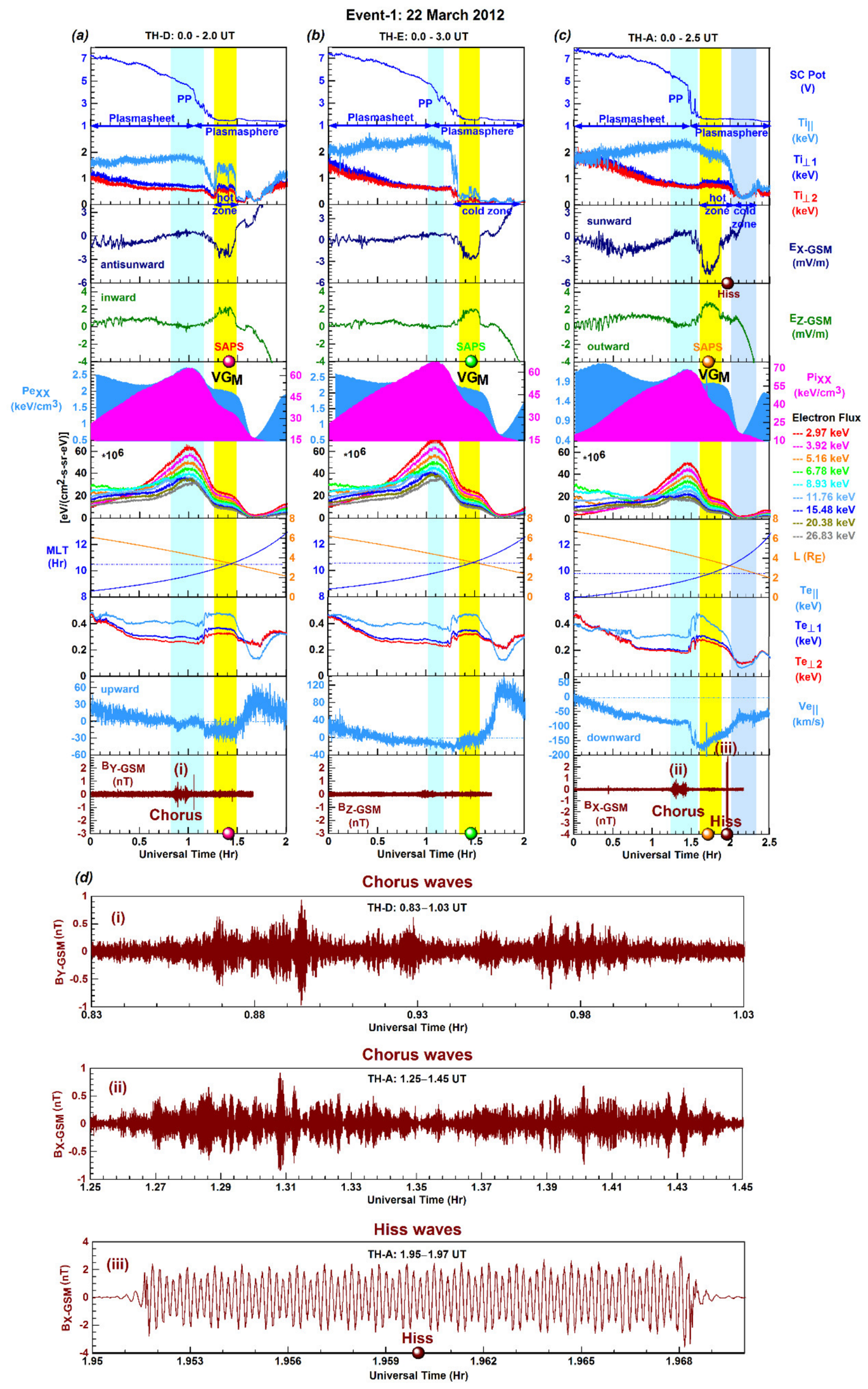
Each line-plot set is constructed with the data of spacecraft potential (SC Pot), ion temperature measured parallel (‖) and perpendicular (⊥) to the magnetic field lines (Ti||, Ti⊥1, Ti⊥12), E field components (EX, EZ), ion and electron pressure (PiXX, PeXX), electron flux measured in the 2.37–26.83 keV range, orbit parameters (L shell, MLT), electron temperature (Te‖, Te⊥1, Te⊥12), field-aligned electron velocity (Ve‖) component, and B field component (BX, BY, BZ). In each line-plot set, we marked the inner-magnetosphere plasmapause (PP) –based on the SC Pot plot– separating the sunward located plasmasheet from the earthward located plasmasphere, and the dayside SAPS E field’s antisunward EX and inward (or earthward) EZ components (dot symbols in color; shaded interval in yellow).
As shown in Figure 7a-c, the inner-magnetosphere PP appeared to be shallow in the thirst two prenoon SAPS events observed by TH-D and TH-E and looked steep in the third prenoon SAPS event observed by TH-A. In each SAPS channel, the antisunward and inward SAPS E field components appeared well-formed and quite small, ~3 mV/m in magnitude, and were observed within the underlying charge separation (depicted by the hot ion and hot electron pressure plots) where the magnetosphere voltage generator (marked as VGM) developed [6].
By translating the duskside SAPS generation processes [6] to the dawnside, we show that the dawnside charge separation formed within the plasmasphere and was created by the hot electron pressure drop at the SAPS channel’s earthward edge and by the hot ion pressure peaking at the PP and dropping across the SAPS channel. Possibly because of the occurrence of weak solar-wind Pdyn increase [59] under the prevailing quiet conditions, the signatures of dayside earthward-directed particle injections did not appear. The absence of earthward-directed particle injections is also clearly shown by the differential ion intensity measured by GEOTAIL (shown in Figure 5a covering the 67.3–538.8 keV energy range) and by the electron flux measured in the 2.97–26.83 keV range by THEMIS (shown in Figure 7a–c). Thus, the absence of dayside earthward-directed particle injections implies that the solar-wind compression of dayside magnetosphere caused only an enhanced plasma convection event [54]. However, due to the compression of dayside magnetosphere by the weakly increased solar-wind Pdyn, the THEMIS-observed electron flux peaked primarily at the PP (see Figure 7a–c) because of the consequential adiabatic enhancement of plasmasheet particles [61]. But this weakly increased solar-wind Pdyn (see Figure 5a) still triggered the necessary conditions for the development of field-aligned temperature anisotropy (T|| > T⊥) via the compression of IMF.
Commonly, the plots of Ti‖ > Ti⊥ and Te‖ > Te⊥ demonstrate field-aligned temperature anisotropy (T‖ > T⊥) generated by the dominating field-aligned energy transport in the plasma [62,63] leading to the generations of whistler-mode waves (observed by THEMIS; see details below) and their related instabilities. These instabilities are key reservoirs of free energy and thus provide efficient bulk plasma heating in a collisionless plasma environment [64,65] that fueled the hot zone. Supporting observations are provided by the Ti‖ > Ti⊥ plots depicting the hot zone as locally increased field-aligned anisotropic Ti within the SAPS channel and the cold zone as locally decreased field-aligned anisotropic Ti. Thus, in the prenoon MLT sector, the inward SAPS E field was observed within the hot zone by TH-D and TH-A, and within the cold zone by TH-E.
Within each SAPS channel, the field-aligned Te anisotropy (Te‖ > Te⊥) peaked and the field-aligned electron drift component (Ve‖; in light blue) became enhanced in the downward direction, as the increased southward IEF E‖ component (< 0; shown in Figure 3a) enhanced the vertical field-aligned electron drift [45]. Thus, the increased field-aligned electron temperature anisotropy (Te‖ > Te⊥) triggered the intensification of whistler-mode chorus waves (shaded interval in cyan) near the PP and in the region of enhanced electron fluxes [66,67,68,69]. These whistler-mode chorus waves are depicted by the plots of BY (marked as (i) in Figure 7a and were observed by TH-D) and of BX (marked as (ii) in Figure 7c and were observed by TH-A). After the third prenoon SAPS detection, TH-A observed whistler-mode plasmaspheric hiss waves (marked as (iii) in Figure 7c) on the earthward side of the PP, between the hot zone and cold zone (see more details below). According to the orbit data, in each prenoon SAPS event, the inward SAPS E field was observed by THEMIS at ~10 MLT and ~4 RE.
Figure 7d shows the expanded narrow UT intervals of these above-mentioned whistler-mode waves. In more detail, we can view the discrete and coherent chorus waves (marked as i and ii) and the broad, structureless and incoherent plasmaspheric hiss waves (marked as iii) observed at ~10 MLT by THEMIS. These chorus waves (i–ii) are depicted by a series of repeating chorus wave elements appearing without any gap between any two adjacent wave elements. These chorus waves’ characteristic signatures include their wave amplitude (≤±1 nT) propagating at group velocity and their wave phase propagating at phase velocity [70]. Meanwhile, the larger amplitude (≤±2.5 nT) hiss waves (marked as iii) depict their characteristic constant frequencies and constant amplitudes [69,71].
3.4.2. SAPS Events-2–3: Midday Outward SAPS on 20 and 22 February 2012
Figure 8a,b illustrate the substorm-time midday SAPS events, observed on 20 and 22 February 2012 by TH-A at ~12 MLT on the duskside, with their respected line-plot sets. Due to the absence of SCM B field measurements, because of the data gap, electromagnetic waves could not be investigated.
Figure 8.
The line-plot sets depict the inner-magnetosphere SAPS channel and its plasma environment (a–c) and (d) the whistler-mode waves developed in (a) Event-2 and (b) Event-3.
Figure 8.
The line-plot sets depict the inner-magnetosphere SAPS channel and its plasma environment (a–c) and (d) the whistler-mode waves developed in (a) Event-2 and (b) Event-3.
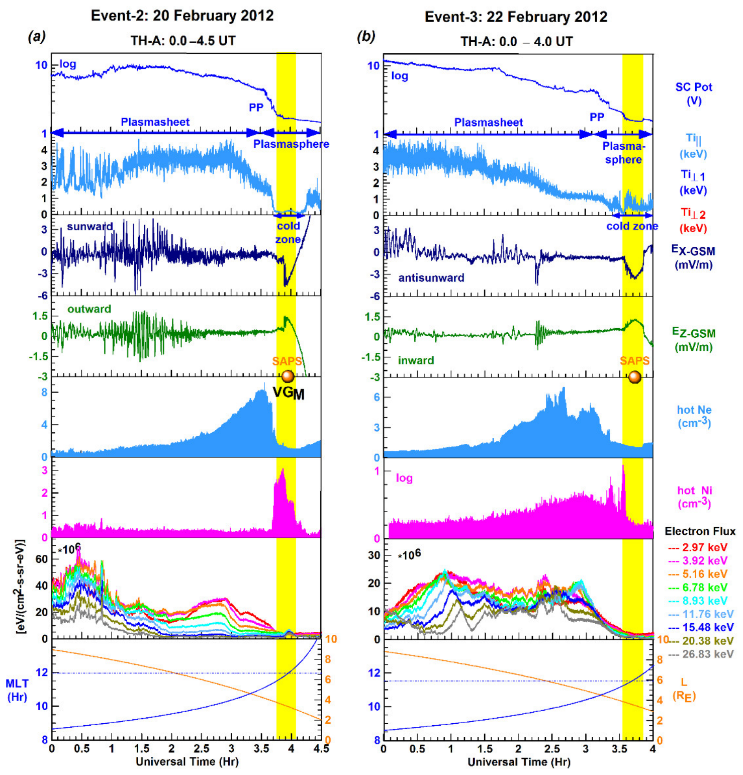
In Figure 8, both line-plot sets show the moderately steep midday plasmapause (PP) and the cold zone appearing in the isotropic (Ti‖ ≈ Ti⊥) ion temperature. Within the cold zone, TH-A observed the small but well-formed antisunward (-) SAPS EX (−4.5 mV/m and −3.5 mV/m) and outward SAPS EZ (1.5 mV/m) components dot symbol in orange; shaded interval in yellow). According to the duskside SAPS generation theory [5,6], the charge separation was created by the hot sunward located electron density drop and by the earthward located hot ion density drop. These small but well-formed near-midday SAPS EX and EZ components appeared within the charge separation in a magnetosphere voltage generator (VGM) setting in Event-2 but were observed at the charge separation’s earthward edge in Event-3 when underlying VGM setting was still evolving and therefore is not marked. Depicted by both hot electron flux line plots, the signatures of earthward-directed dayside hot electron injections are well visible within the 8–9 MLT sector of the plasmasheet. According to the orbit data, TH-A observed these two midday SAPS events at ~11.5 MLT and ~3.5 RE.
3.5. M-I Conjugate Substorm-Time SAPS Phenomena Observed on 3 Marh 2012
3.5.1. SAPS Events-4: Midday Outward SAPS Observed by THEMIS
Figure 9a–c illustrate the three midday SAPS channels (dot symbols in colors; shaded interval in yellow) observed by THEMIS on 3 March 2012 in Event-4. Arranged in increasing SAPS UT detection order, the midday SAPS channel was observed just after 2.5 UT by TH-E and TH-D and soon after 3.0 UT by TH-A.
Due to the increased plasma convection (indicated by the increased IEF; see details below), the plasmapause (PP) –that is a corotation-convection boundary [72]—appeared to be steep and sharp. Furthermore, the ion temperature was field-aligned anisotropic (Ti‖ > Ti⊥) within the plasmasheet due to the temporarily increased convection evidenced by the duskward IEF EY (up to ~2 mV/m; see Figure 3d) and southward IEF E‖ (up to ~1.5 mV/m; see Figure 3d). Near and on the earthward side of the PP (i.e., in the plasmasphere), the ion temperature was low and isotropic (Ti‖ ≈ Ti⊥). Thus, THEMIS observed the midday SAPS in the cold zone. There, the antisunward and outward SAPS E field components were small in magnitude (EX ≈ −3 mV/m; EZ ≈ 2 mV/m) but well formed. Oppositely to the Ti plots, the electron temperature was field-perpendicular anisotropic (Te⊥ > Te‖) and locally increased within the isotropic Ti regime of the cold zone.
Although the charge separation appears clearly in each midday SAPS channel, only the TH-E-observed midday SAPS channel shows the SAPS EX and EZ field components appearing within the charge separation and in a magnetosphere voltage generator (VGM) setting. Possibly, the following two SAPS channels were still in progress. By applying the duskside SAPS development theory [5,6], we show with Figure 9a that the charge separation was created by the hot electron density drop close to the sunward edge of the PP and by the hot ion density drop across the midday SAPS channel. Within the charge separation, the magnetosphere voltage generator (VGM) developed. Since Figure 9b,c show charge separation development still in progress, their respective VGM settings were not fully developed and therefore we did not mark them.
In each midday SAPS channel, the hot electron flux measurements depict the signatures of earthward-directed hot electron surges observed by THEMIS within the plasmasheet. These provide further observational evidence that the charge separation was triggered by the earthward-directed hot plasma surges traveling from the solar-wind-exposed dayside magnetosphere (observed by GEOTAIL; see Figure 5d) and reaching the plasmasheet (observed by THEMIS). According to the orbit data, THEMIS observed these three midday SAPS events between 11.5 and 12 MLT and ~3.5 RE.
In the last TH-A-observed midday SAPS channel, Ve|| decreased within the plasmasphere and whistler-mode hiss waves (marked as (i)) were detected within the isotropic (Ti|| ≈ T⊥) cold zone. Figure 9d shows the expanded narrow UT interval of the above-mentioned whistler-mode hiss waves (marked as i). In this way, we can illustrate the broad, structureless and incoherent plasmaspheric hiss waves observed at ~11.5 MLT by TH-A.
3.5.2. Postnoon (13 LT) Topside-Ionosphere SAPS Event Observed by DMSP
Figure 10 and Figure 11 show the M-I conjugate midday SAPS phenomenon’s ionospheric component observed by DMSP F16 in the topside ionosphere soon after the inner-magnetosphere THEMIS observations (shown in Figure 10) and later on (shown in Figure 11) on 3 March 2012.
In Figure 10a, the northern-hemisphere geographic map depicts the footprints of these three THEMIS satellites taken during the midday SAPS Event-4 on 3 March 2012 along with the mapped-down SAPS E field locations (dot symbols in colors) in the Asian sector and the DMSP F16-03 ascending and descending passes (in cyan). Then, F16 observed the SAPS flow channel (symbol dot in cyan) and FC-0 (square symbol in cyan) near Alaska soon after local midday and the polar cap plasma increases (one is indicated as diamond symbol in cyan) in the Asian sector before midday. We note here that FC-0 specifies the flow channel of return convection flow of the polar convection pattern based on previously established classification [73].
In Figure 10b, the northern-hemisphere TEC map was constructed with GNSS TEC data covering the 3–4 UT time-period. Then, the third midday inner-magnetosphere SAPS channel was observed at 3.15 UT (by TH-A) and the midday topside-ionosphere SAPS flow was observed shortly after, at 3.43 UT (by F16). Although these 3.15 UT and 3.43 UT values indicate a close M-I correlation, the M-I conjugate SAPS locations plotted (dot symbols in colors) illustrate that all these midday SAPS detections mapped down to different regions of the SED plume base. While the three inner-magnetosphere SAPS E fields (observed by THEMIS) mapped down to ~60° N in the (120–140)° E sector, the topside-ionosphere SAPS flow channel was observed by F16 at higher latitude (~71° N) and longitude (~180° E). Thus, the THEMIS-observed SAPS E fields drove at lower latitudes (~60° N) the SED plume plasma sunward. Meanwhile, the F16-observed SAPS flow convected the SED plume plasma at higher latitudes (~71° N) towards the polar cap region, where F16 observed polar plasma density increases (one is indicated as diamond symbol in cyan). Further illustration is provided by the polar TEC plot depicting the SED plume plasma near the polar cap entry, where the polar plasma density increases were observed (one is indicated as diamond symbol in cyan) and the SAPS locations (dot symbols in colors) at the SED plume base in the midday (in LT) sector but at different latitudes.
In Figure 10c, the line-plot sets illustrate the F16-measured variables of electron density (Ne), electron and ion temperature (Te and Ti), cross-track drift components (VHOR and VVER), magnetic deflection component (δBZ), and Poynting flux (S||). Here, we marked the postnoon and prenoon auroral zones along with the polar cap region. Progressing from top to bottom, the Ne plot depicts the SED feature in the postnoon (MLT, LT) sector and the polar plasma density increases (shaded interval in light magenta) that were convected antisunward by the underlying antisunward (-) polar convection (VHOR ≈ −800 m/s). According to the temperature variation, Te peaked (at ~6000 K) within FC-0 (shaded interval in cyan) where the polar convection return flow maximized (at VHOR ≈ 1500 m/s) within the postnoon auroral zone. But Te remained low (~3000 K) in the weak SAPS channel (VHOR ≈ 800 m/s; shaded interval in yellow) that was possibly quite newly formed and appeared just poleward of the SED feature and with no underlying plasma density trough in a voltage generator setting (see details below). However, Te increased (up to ~5000 K) in the polar cap, where the antisunward (-) convection was strong (VHOR ≈ −800 m/s) and where the upward drift maximized (at VVER ≈ 800 m/s). Implying a voltage generator setting [74,75], the ionosphere poleward SAPS E field was created by the mapping down of inner-magnetosphere outward SAPS E field. This is further illustrated with the δBZ line plot that depicts the flow of weak ↓R2 current (δBZ ≈ 80 nT) into the newly-formed SAPS channel, where the earthward energy deposition was minimal (S|| ≈ 2 mW/m2), and the connection of significantly stronger ↓R2-↑R1 currents (δBZ ≈ 160 nT) by the poleward-directed Pedersen current in the return flow channel (FC-0) receiving ~7 mW/m2 earthward energy deposition from the magnetosphere. According to the orbit data, F16 observed the weak SAPS flow soon after midday (12.85 LT), the strong return flow at almost midday (12.27 LT), and the polar cap plasma density increases before midday (10.98 LT).
3.5.3. Prenoon (11 LT) Topside-Ionosphere SAPS Event Observed by DMSP
Figure 11 was constructed the same way as Figure 10 and illustrates how the newly formed midday SAPS flow in the topside ionosphere’s postnoon sector (shown in Figure 10c) became further evolved later on in the prenoon (11 LT) sector (shown in Figure 11c).
In Figure 11a, the northern-hemisphere map shows that F16 observed this prenoon SAPS flow channel (dot symbol in cyan) together with FC-0 (square symbol in cyan) and polar plasma density increase (diamond symbol in cyan) along the next ascending pass (F16-04) in the Asian sector at higher geographic latitudes. According to the TEC map of Figure 11b, both flow channels (SAPS and FC-0; circled in white) were in a low TEC region (6–11 TECU; shades of green) near the SED plume’s northern edge (11–15 UT; shades of orange). As the SED plume progressed towards the polar cap region, F16 observed the plasma density increase (diamond symbol in cyan; circled in white) in the polar cap. Further illustration is provided by the polar TEC plot depicting the prenoon SAPS at ~11 LT and FC-0 near the SED plume entering the polar cap, and the polar plasma density increase within the polar cap.
Figure 11c shows a set of line plots constructed as Figure 10c. As shown, this more evolved and well-formed prenoon (~11 LT) SAPS flow (VHOR ≈ 900 m/s) appeared within a well-formed plasma density trough (T; shaded interval in yellow) where Te increased up to ~4500 K. Meanwhile, the auroral return flow (FC-0; shaded interval in cyan) also appeared stronger (VHOR ≈ 1900 m/s) than earlier (VHOR ≈ 1500 m/s shown in Figure 10c) and within the low density postnoon (in MLT) auroral zone, where the upward drift peaked (VVER ≈ 700 m/s) and Te maximized at ~6000 K. As indicated by the polar plasma density increases (shaded interval in light magenta), F16 observed the edge of SED plume plasma that was driven into the polar cap region by the strong underlying antisunward (-) polar convection (VHOR ≈ −900 m/s). The flow of weak ↓R2 (δBZ ≈ 120 nT) into the SAPS channel implies that currents started flowing in the voltage generator, while the stronger ↓R2 and ↑R1 currents (δBZ ≈ 280 nT) connected via the poleward-directed Pedersen current in the return flow channel (FC-0). Illustrated by the S‖ plot, both the SAPS channel and the polar cap region received minimal earthward energy (S‖ ≈ 3 mW/m2) while earthward energy deposition maximized (at S‖ ≈ 15 mW/m2) within the auroral return flow (FC-0). According to the orbit data, F16 observed this better developed SAPS flow before midday (10.88 LT), the strong return flow earlier (10.25 LT), and the polar plasma density increase in the local morning sector (8.09 LT).
4. Discussion
4.1. Inner-Magnetosphere SAPS Channel Development in the Midday and Prenoon Sectors
We investigated the development of inner-magnetosphere SAPS channel on the dayside, near the magnetic equatorial plane, and close to magnetic noon on the duskside (at ~12 MLT) and on the dawnside (~10 MLT), where these SAPS channels were observed by THEMIS in their respective magnetosphere voltage generator (VGM) settings. Although the SAPS E field components appeared well formed, they were quite small in magnitude (~2–3 mV/m). Furthermore, their underlying dayside geophysical mechanisms were very different from their nightside counterparts driven by nighttime magnetotail-reconnection-related processes. We found that on the dayside and in the magnetic prenoon and midday sectors, where the solar wind was highly Alfvenic, the unfolding solar-wind dynamic pressure increases (Pdym shown in Figure 3a–d and Figure 5a–d) drove sometimes daytime earthward-directed hot plasma surges (see Figure 5a,c) and sometimes daytime earthward-directed hot particle injections (see Figure 5b,c). Both the hot plasma surges and the hot particle injections led to charge separation in a VGM setting and thus, were able to onset daytime SAPS development on the dayside (see Figure 1).
In order to explain how the dayside solar-wind dynamic pressure increase set off SAPS development on the dayside, first, we briefly describe the fast-time duskside SAPS development’s relevant features and then translate the main duskside driver mechanisms to the prenoon and midday sectors.
According to the fast-time duskside SAPS development theory [5,6]), magnetotail-reconnection-related earthward-directed hot particle injections initiate duskside SAPS development that is an integral part of the SCW2L system [75] since the SCW2L system demands the closure of oppositely directed ↑R1–↓R2 FACs at the leading duskward (or westward) edge of the SCW. Such current closure occurs near the inner-magnetosphere plasmapause via meridional partial ring currents and requires an outward E field that is provided by the inner-magnetosphere outward SAPS E field. Mapped down to the duskside ionosphere, the SCW appears as an auroral bulge, and its leading westward (or duskward) edge propagates westward (or duskward). This phenomenon is known as the westward traveling surge (WTS) [8,9,10]. Furthermore, the westward (or duskward) propagating auroral bulge/WTS is associated with an enhanced auroral westward electrojet (WEJ) that is dominated by ↑R1 currents in its active westward (or duskward) propagating region (see Figure 9 in [8]). Thus, current closure in the ionosphere SAPS channel occurs at the enhanced WEJ’s leading westward (or duskward) edge, where the enhanced ↑R1 FACs associated with the auroral WEJ connect with the weaker subauroral-EEJ-associated ↓R2 FACs flown into the subauroral region (see Figure 2 in [76]).
Based on the above-described M-I conjugate duskside SAPS development on the nightside, we invoke the important roles of solar wind dynamic pressure (Pdyn) increases and dayside auroral electrojets (AEJs) in the M-I conjugate daytime (prenoon/midday) SAPS channel’s development. Based on recent statistical investigations [77], dayside AEJs directly respond to solar-wind dynamic pressure increases as prenoon eastward electrojet (EEJ) increases on the dawnside and midday/postnoon WEJ increases on the duskside. Meanwhile, the reversal of dayside AEJ occurs at magnetic midday (see Figure 11 in [77]). We put forward here that possibly such dayside solar-wind Pdyn and dayside AEJ increases triggered the development of dayside M-I conjugate SAPS under study: in a prenoon EEJ scenario on the dawnside and in a midday WEJ scenario on the duskside. For further supporting our dayside explanations, we provide additional observational evidence with AMPERE δBFIT vector polar plots showing a midday/postnoon WEJ scenario in Figure 12 and a prenoon scenario in Figure 13.
Figure 12 is constructed for the 20 February 2012 midday SAPS Event-2 (see also Figure 8a), observed by TH-A, and illustrates the MLT versus GLAT vector polar map of δBFIT generated for 4 UT when TH-A observed the outward SAPS E field at midday. We marked the mapped-down SAPS channel location as dot symbol in orange. Located in the postnoon 12–14 MLT sector on the duskside, we marked the stronger clockwise auroral WEJ (in red) propagating toward magnetic noon and the weaker anticlockwise EEJ (in blue) appearing at subauroral latitudes. Shown by the large-scale FACs marked with the vertical arrows, the meridional current closer took place at the duskside WEJ’s leading noontime edge between the ↑R1 currents (in red) associated with the stronger midday/postnoon WEJ and ↓R2 currents (in blue) flown into the midday/postnoon subauroral region and associated with the weaker midday/postnoon EEJ. We also note that this vector map shows quite clearly the reversal of dayside AEJ at magnetic midday first reported [77] from a duskside clockwise WEJ to a dawnside anticlockwise EEJ.
Figure 13 is constructed for the 22 March 2012 prenoon SAPS Event-1 (see also Figure 7a–c) and shows the MLT versus GLAT polar δBFIT vector map that was generated for 2 UT. Then, TH-A observed the dawnside inner-magnetosphere SAPS channel that mapped down to the prenoon sector (marked as dot symbol in orange). We marked on the dawnside the stronger anticlockwise auroral EEJ (in red) dominated by stronger ↓R1 currents and propagating toward magnetic noon and the weaker clockwise WEJ (in blue) dominated by weaker ↑R2 currents and appearing at subauroral latitudes. Illustrated by the large-scale FACs marked with the vertical arrows, the meridional current closer took place at the dawnside EEJ’s leading prenoon edge between the weaker ↑R2 currents (in blue) extending into the subauroral region and associated with the weaker prenoon EEJ and the stronger ↓R1 currents (in red) associated with the stronger prenoon auroral WEJ.
4.2. Dayside Hot Zone and Cold Zone
A significant finding of this study is the development of inner-magnetosphere daytime SAPS channel sometimes within the hot zone and sometimes within the cold zone. Recent studies highlighted first the strong association of nighttime inner-magnetosphere hot zone and nighttime inner-magnetosphere outward SAPS/SAID E field near the plasmapause [1]. Previous studies explained nighttime plasmaspheric heating in the region of nighttime plasmapause with electromagnetic ion cyclotron (EMIC) waves [78]) and fast magnetosonic (MS) waves [79] generated in the ring current core region and also with lower hybrid waves [80,81] generated near the ring current inner (earthward) edge. However, the hot zone’s sharp boundary near the plasmapause favors the EMIC-wave-generation scenario created by the interaction of earthward travelling hot ring current ions (from the nightside reconnection region while crossing perpendicularly the vertical magnetic field lines) and cold electrons near the plasmapause. Therefore, the nightside plasma temperature is field-perpendicular anisotropic (T⊥ > T‖) because of the transport of energy stored in the earthward traveling hot ions [78,82,83]. When the field-perpendicular ion anisotropy (Ti⊥ > Ti‖) is strong enough, EMIC waves develop via ion cyclotron resonant instability that requires such (Ti⊥ > Ti‖) ion temperature anisotropy [84,85] and can lead to bulk plasma heating via wave-particle interaction fueling the hot zone [18].
Opposite to the above-described hot-zone-related nighttime EMIC wave scenario, our daytime hot-zone related whistler-mode scenarios demonstrate (in Figure 7) that the compression of dayside magnetosphere by dayside solar-wind dynamic pressure pulses created field-aligned Ti (Ti‖ > Ti⊥) and Te (Te‖ > Te⊥) anisotropy via field-aligned plasma acceleration [45]. Such field-aligned acceleration was provided by the increased IEF E‖ component convecting the dayside plasma along the magnetic field lines. These observations are in agreement with recent studies [69,86] reporting that the sudden intensifications of solar wind dynamic pressure triggers (i) the development of new or (ii) the intensity increase of already existing whistler-mode chorus waves via the sudden compression of the dayside magnetosphere. Recently, it was suggested [86] that the source of free energy for chorus wave generation is provided by the anisotropy developed in the electron population. We show in this study that when the electron (Te‖ > Te⊥) anisotropy was strong enough, whistler-mode chorus waves (see Figure 7d) became generated. According to more recent studies [87,88], whistler-mode chorus waves can implicitly participate in heating processes. We speculate that whistler-mode chorus waves led to bulk plasma heating via wave-particle interaction fueling the plasmaspheric hot zone characterized by field-aligned Ti (Ti‖ > Ti⊥) anisotropy on the dayside. Under magnetically quiet conditions, THEMIS observed these hot-zone-related whistler-mode scenarios (shown in Figure 7a–c) near the magnetic equatorial plane within the inner magnetosphere and near the midday plasmapause. This is where chorus waves are generated [84,89], regardless of the underlying geomagnetic activity, particularly at magnetic noon [86,90,91].
Our cold-zone scenarios show in Figure 7, Figure 8 and Figure 9 that the cold zone was created sometimes by the minimized isotropic Ti (Ti⊥ ≈ Ti‖) that was sometimes accompanied by field-perpendicular (Te⊥ > Te||) anisotropic Te (see Figure 9c). The cold-zone-related Ti and Te regimes were observed earthward of the hot zone (see Figure 7a-c) or near the plasmapause in the hot zone’s absence (see Figure 7a,b and Figure 8a–c). But sometimes, in the cold zone, the minimized isotropic Ti (Ti⊥ ≈ Ti‖) was accompanied by maximized field-perpendicular anisotropic Te (Te⊥ > Te‖) near the plasmapause (see Figure 9a–c). Sometimes within the cold zone, where the underlying Te anisotropy was field-perpendicular (Te⊥ > Te‖; see Figure 9a–c), whistler-mode hiss waves were also observed by THEMIS (see Figure 9c-d). These hiss waves were possibly generated by the whistler-mode chorus waves that propagated from their original inner magnetosphere locations (where THEMIS observed the chorus waves) to the plasmapause and then evolved into hiss waves [92,93].
4.3. Dayside SED Plume
In the absence of cold plasma density THEMIS measurements, we used SC Potential line plots that do not show the inner-magnetosphere SED plume, which develops near the inner-magnetosphere plasmapause where the combination of convection E field and SAPS E field strips away the outer layer of the plasmaspheric plasma creating SED plume also called erosion plume [94]. But all the northern-hemisphere TEC maps constructed show (see Figure 6) that the THEMIS-observed daytime SAPS E field mapped down to the midday SED plume base. There, sunward SAPS flow drove the SED plume plasma sunward, toward the polar cap’s entry region. This was further illustrated with loosely correlated M-I conjugate THEMIS-DMSP observations. DMSP F16 observed near local midday (i) the strong sunward auroral return flow (specified as FC-0) [73] implying the strong polar convection and (ii) the polar cap plasma density increases at the polar cap’s entry region along with their underlying increased polar convection (see Figure 10). In this strong polar convection environment, DMSP F16 observed both the SED feature and the nearby newly formed and weak sunward SAPS flow. Later on (see Figure 11), DMSP F16 observed a similar scenario depicting a stronger and old (i.e., previously developed) sunward SAPS flow at higher latitude.
5. Conclusions
In this study, we investigated the inner-magnetosphere SAPS channel’s development and plasma environment near the magnetic equatorial plane and close to magnetic midday in order to get a better understanding of the midday subauroral geospace. From the observational evidence provided, we documented the following significant findings:
-
The daytime inner-magnetosphere SAPS E field was observed by THEMIS sometimes:
- -
- within the hot zone characterized by field-aligned temperature anisotropy (T‖ > T⊥) and fueled implicitly by whistler-mode chorus waves developed because of the increased field-aligned IEF E‖ field,
- -
- within the cold zone characterized by ion temperature isotropy (Ti‖ ≈ Ti⊥).
- Dayside fast-time SAPS development, unfolding under Alfvenic solar wind conditions in the inner magnetosphere, was set off by solar-wind dynamic pressure increases that drove daytime earthward-directed hot plasma surges and/or particle injections leading to charge separation in the prenoon sector on the dawnside or in the midday sector on the duskside.
- The inner-magnetosphere midday/prenoon SAPS channel was observed within the duskside/dawnside charge separation and in a magnetosphere voltage generator (VGM) setting, similarly to the nighttime duskside or dawnside counterpart.
- The inner-magnetosphere daytime SAPS channel mapped down from the magnetic equatorial plane to the noontime SED plume base in the ionosphere.
- In the ionosphere, SAPS development unfolded in an EEJ scenario in the dawnside’s prenoon sector or in a WEJ scenario in the duskside’s postnoon sector.
Finally, from the above-listed significant findings we conclude for the daytime SAPS events investigated that (1) the development of M-I conjugate daytime SAPS channel (i) was set off by the increased solar-wind dynamic pressure compressing the dayside magnetosphere and (ii) could be explained by invoking the nightside fast-time SAPS development theory and by translating the nighttime SAPS generation mechanisms to the dayside (prenoon and noon sectors), and (2) the hot zone’s dayside development was due to the whistler-mode chorus waves that implicitly participated in the underlying heating processes. In order to specify the possible underlying heating processes, further detailed studies and investigations are required.
Author Contributions
Conceptualization, I.H.; methodology, I.H.; software, I.H. and B.L.; validation, I.H. and B.L.; formal analysis, I.H.; investigation, I.H.; resources, B.L.; data curation, I.H.; writing—original draft preparation, I.H.; writing—review and editing, B.L. and I.H.; visualization, I.H.; supervision, B.L.; project administration, B.L.; funding acquisition, B.L. All authors have read and agreed to the published version of the manuscript.
Funding
This research was funded by the United States Office of Naval Research, grant number N62909-23-1-2057.
Data Availability Statement
THEMIS, GEOTAIL and OMNI data sets can be accessed online through https://cdaweb.gsfc.nasa.gov/cdaweb/istp_public/ (last accessed on 8 July 2026), DMSP and TEC data set can be accessed online through http://cedar.openmadrigal.org (last accessed on 8 July 2026) AMPERE imagery can be accessed online through, https://ampere.jhuapl.edu/browse-sandbox/ (last accessed on 8 July 2026) SuperMAG provided various types of substorm lists can be accessed online from the SuperMAG substorm lists through, https://supermag.jhuapl.edu/substorms/ (last accessed on 8 July 2026).
Acknowledgments
We gratefully acknowledge the CEDAR Archival Madrigal Database for the DMSP and GNSS TEC data and the NASA Coordinated Data Analysis Web (CDAWeb) for the THEMIS, GEOTAIL and OMNI datasets. We also gratefully acknowledge the PC index that is derived in partnership between the Arctic and Antarctic Research Institute (AARI, Russian Federation) and the National Space Institute, Technical University of Denmark (DTU, Denmark) and the World Data Center for Geomagnetism at Kyoto (http://wdc.kugi.kyoto-u.ac.jp/wdc/Sec3.html) for providing the AE, AL and Kp indices. We also gratefully acknowledge the AMPERE images and thank the AMPERE team and the AMPERE Science Data Center for providing data/imagery products derived from the Iridium Communications constellation, enabled by support from the National Science Foundation.
Conflicts of Interest
The authors declare no conflicts of interest.
Abbreviations
The following abbreviations are used in this manuscript:
| ACE | Advance Composition Explorer |
| AMPERE | Active Magnetosphere and Planetary Electrodynamics Response Experiment |
| AEJ | Auroral Electrojet |
| DMSP | Defense Meteorological Satellite Program |
| EEJ | Eastward Electrojet |
| E field | Electric field |
| EMIC | Electromagnetic Ion Cyclotron |
| FACs | Field-Aligned Currents |
| FC | Flow Channel |
| GLAT | Geographic Latitude |
| GNSS | Global Navigation Satellite System |
| GSM | Geocentric Solar Magnetospheric |
| IEF | Interplanetary Electric Field |
| IMF | Interplanetary Magnetic Field |
| LT | Local Time |
| M-I | Magnetosphere-Ionosphere |
| MLAT | Magnetic Latitude |
| MLT | Magnetic Local Time |
| MS | Magnetosonic |
| R1 | Region 1 |
| R2 | Region 2 |
| SAPS | Sub-Auroral Polarization Streams |
| SCW | Substorm Current Wedge |
| SCW2L | Substorm Current Wedge 2 Loop |
| SED | Storm Enhanced Densities |
| TEC | Total Electron Content |
| TECU | Total Electron Content Unit |
| THEMIS | Time History of Events and Macroscale Interactions during Substorms |
| TH-A | THEMIS-A |
| TH-D | THEMIS-D |
| TH-E | THEMIS-E |
| UT | Universal Time |
| VGM | Magnetosphere Voltage Generator |
| WEJ | Westward Electrojet |
| WTS | Westward Traveling Surge |
References
- Mishin, E.; Streltsov, A. Mesoscale and Small-Scale Structure of the Subauroral Geospace. In Ionosphere Dynamics and Applications; Huang, C., Lu, G., Eds.; Geophysical Monograph Series; Space Physics and Aeronomy Collection Volume 3; American Geophysical Union: Washington DC, USA, 2021; pp. 135–154. [Google Scholar] [CrossRef]
- Mishin, E.V.; Streltsov, A.V. Multiscale Electrodynamics of Subauroral Flows and Arcs: A Major Paradigm Shift. Space Sci. Rev. 2026, 222, 1–89. [Google Scholar] [CrossRef]
- Foster, J.C.; Burke, W.J. SAPS: A new categorization for sub-auroral electric fields. Eos Trans. Am. Geophys. Union 2002, 83, 393–394. [Google Scholar] [CrossRef]
- Dungey, J.W. Effects of electromagnetic perturbations on particles trapped in the radiation belts. Space Sci. Rev. 1965, 4, 199–222. [Google Scholar] [CrossRef]
- Mishin, E. SAPS onset timing during substorms and the westward traveling surge. Geophys. Res. Lett. 2016, 43, 6687–6693. [Google Scholar] [CrossRef]
- Mishin, E.; Nishimura, Y.; Foster, J. SAPS/SAID revisited: A causal relation to the substorm current wedge. J. Geophys. Res. Space Phys. 2017, 122, 8516–8535. [Google Scholar] [CrossRef]
- Sergeev, V.A.; Nikolaev, A.V.; Tsyganenko, N.A.; Angelopoulos, V.; Runov, A.V.; Singer, H.J.; Yang, J. Testing a two-loop pattern of the substorm current wedge (SCW2L). J. Geophys. Res. 2014, 119, 947–963. [Google Scholar] [CrossRef]
- Kepko, L.; McPherron, R.; Amm, L.O.; Apatenkov, S.; Baumjohann, W.; Birn, J.; Lester, M.; Nakamura, R.; Pulkkinen, T.I.; Sergeev, V. Substorm Current Wedge Revisited. Space Sci. Rev. 2015, 190, 1–46. [Google Scholar] [CrossRef]
- Wei, D.; Zhang, F.; Yang, J.; Wang, W.; Sun, W.; Cui, J.; Angelopoulos, V. A magnetospheric driver of westward traveling surge: Plasmasheet bubble. Geophys. Res. Lett. 2021, 48, e2021GL095539. [Google Scholar] [CrossRef]
- Wei, D.; Yang, J.; Liu, C.; Zhang, F.; Wang, W.; Sun, W. Successive westward traveling surges driven by sequential plasma-sheet bubble injections. Geophys. Res. Lett. 2022, 49, e2022GL100774. [Google Scholar] [CrossRef]
- Horvath, I.; Lovell, B.C. Investigating the coupled magnetosphere-ionosphere-thermosphere (M-I-T) system’s responses to the 20 November 2003 superstorm. J. Geophys. Res. Space Phys. 2021, 126, e2021JA029215. [Google Scholar] [CrossRef]
- Lyons, L.R.; Lee, D.-Y.; Wang, C.-P.; Mende, S.B. Global auroral responses to abrupt solar wind changes: Dynamic pressure, substorm, and null events. J. Geophys. Res. 2005, 110, A08208. [Google Scholar] [CrossRef]
- Horvath, I.; Lovell, B.C. Multi-point satellites observed dawnside Subauroral Polarization Streams (SAPS) developed on a short timescale under weak-storm and non-storm substorm conditions. J. Geophys. Res. Space Phys. 2025, 130, e2025JA033755. [Google Scholar] [CrossRef]
- Foster, J.C. Storm time plasma transport at middle and high latitudes. J. Geophys. Res. 1993, 98(A2), 1675–1689. [Google Scholar] [CrossRef]
- Foster, J.C.; Coster, A.J.; Erickson, P.J.; Rich, F.J.; Sandel, B.R. Stormtime observations of the flux of plasmaspheric ions to the dayside cusp/magnetopause. Geophys. Res. Lett. 2004, 31, L08809. [Google Scholar] [CrossRef]
- Foster, J.C.; Coster, A.J.; Erickson, P.J.; Holt, J.M.; Lind, F.D.; Rideout, W.; et al. Multiradar observations of the polar tongue of ionization. J. Geophys. Res. 2005, 110, A09S31. [Google Scholar] [CrossRef]
- Foster, J.C.; Zou, S.; Heelis, R.A.; Erickson, P.J. Ionospheric storm enhanced density plumes. In Space Physics and Aeronomy Collection Volume 3: Lonosphere Dynamics and Applications, 1st ed.; Huang, C.S., Lu, G., Eds.; American Geophysical Union: Washington DC, USA, 2021; pp. 117–126. [Google Scholar] [CrossRef]
- Gringauz, K.I.; Bezrukikh, V.V. Asymmetry of the Earth’s plasmasphere in the direction noon-midnight from Prognoz and Prognoz-2 data. J. Atmos. Terr. Phys. 1976, 38, 1071–1076. [Google Scholar] [CrossRef]
- Tsurutani, B.T.; Smith, E.J. Postmidnight chorus: A substorm phenomenon. J. Geophys. Res. 1974, 79, 118–127. [Google Scholar] [CrossRef]
- Li, W.; Bortnik, J.; Thorne, R.M.; Angelopoulos, V. Global distribution of wave amplitudes and wave normal angles of chorus waves using themis wave observations. J. Geophys. Res. 2011, 116, A12205. [Google Scholar] [CrossRef]
- Li, W.; Thorne, R.M.; Bortnik, J.; Reeves, G.D.; Kletzing, C.A.; Kurth, W.S.; et al. An unusual enhancement of low-frequency plasmaspheric hiss in the outer plasmasphere associated with substorm-injected electrons. Geophys. Res. Lett. 2013, 40, 3798–3803. [Google Scholar] [CrossRef]
- Tsurutani, B.; Falkowski, B.; Pickett, J.; Verkhoglyadova, O.; Santolík, O.; Lakhina, G. Extremely intense ELF magnetosonic waves: A survey of polar observations. J. Geophys. Res. Space Phys. 2014, 119, 964–977. [Google Scholar] [CrossRef]
- Boudouridis, A.; Lyons, L.; Zesta, E.; Weygand, J.; Ribeiro, A.; Ruohoniemi, J. Statistical study of the effect of solar wind dynamic pressure fronts on the dayside and nightside ionospheric convection. J. Geophys. Res. Space Phys. 2011, 116, A10233. [Google Scholar] [CrossRef]
- Yu, J.; Li, L.Y.; Cao, J.B.; Reeves, G.D.; Baker, D.N.; Spence, H. The influences of solar wind pressure and interplanetary magnetic field on global magnetic field and outer radiation belt electrons. Geophys. Res. Lett. 2016, 43, 7319–7327. [Google Scholar] [CrossRef]
- Wang, H.; Lühr, H. Effects of solar illumination and substorms on auroral electrojets based on CHAMP observations. J. Geophys. Res. Space Phys. 2021, 126, e2020JA028905. [Google Scholar] [CrossRef]
- Nakano, S.; Ueno, G.; Ohtani, S.; Higuchi, T. Impact of the solar wind dynamic pressure on the Region 2 field-aligned currents. J. Geophys. Res. 2009, 114, A02221. [Google Scholar] [CrossRef]
- Sibeck, D.G.; Angelopoulos, V. THEMIS science objectives and mission phases. Space Sci. Rev. 2008, 141, 35–59. [Google Scholar] [CrossRef]
- Bonnell, J.; Mozer, F.S.; Delory, G.T.; Hull, A.J.; Ergun, R.E.; Cully, C.M.; Angelopoulos, V.; Harvey, P.R. The Electric Field Instrument (EFI) for THEMIS. Space Sci. Rev. 2008, 141, 303–341. [Google Scholar] [CrossRef]
- McFadden, J.P.; Carlson, C.W.; Larson, D.; et al. The THEMIS ESA Plasma Instrument and In-flight Calibration. Space Sci. Rev. 2008, 141, 277–302. [Google Scholar] [CrossRef]
- McFadden, J.P.; Carlson, C.W.; Larson, D.; et al. THEMIS ESA First Science Results and Performance Issues. Space Sci. Rev. 2008, 141, 477–508. [Google Scholar] [CrossRef]
- Roux, A.; Le Contel, O.; Coillot, C.; et al. The Search Coil Magnetometer for THEMIS. Space Sci. Rev. 2008, 141, 265–275. [Google Scholar] [CrossRef]
- Nishida, A. The geotail mission. Geophys. Res. Lett. 1999, 421, 2871–2873. [Google Scholar] [CrossRef]
- Williams, D.J.; McEntire, R.W.; Schlemm, I.I.; Liu, A.T.Y.; Gloeckler, G.; Christon, S.P.; Gliem, F. Geotail energetic particles and ion composition instrument. J. Geomagn. Geoelectr. 1994, 46, 39–57. [Google Scholar] [CrossRef]
- Frank, L.A.; Ackerson, K.L.; Paterson, W.R.; Lee, J.A.; English, M.R.; Pickett, G.L. The comprehensive plasma instrumentation (CPI) for the Geotail spacecraft. J. Geomagn. Geoelectr. 1994, 46, 23–37. [Google Scholar] [CrossRef]
- Kokubun, S.; Yamamoto, T.; Acuna, M.H.; Hayashi, K.; Shiokawa, K.; Kawano, H. The GEOTAIL Magnetic Field Experiment. J. Geomagn. Geoelectr. 1994, 46, 7–21. [Google Scholar] [CrossRef]
- Rich, F.J.; Hairston, M. Large-scale convection patterns observed by DMSP. J. Geophys. Res. 1994, 99, 3827–3844. [Google Scholar] [CrossRef]
- Rich, F.J.; Bono, J.M.; Burke, W.J.; Gentile, L.C. A space-based proxy for the Dst index. J. Geophys. Res. Space Phys. 2007, 112, A05211. [Google Scholar] [CrossRef]
- Huang, C.Y.; Burke, W.J. Transient sheets of field-aligned current observed by DMSP during the main phase of a magnetic superstorm. J. Geophys. Res. 2004, 109, A06303. [Google Scholar] [CrossRef]
- Huang, C.Y.; Su, Y.; Sutton, E.K.; Weimer, D.R.; Davidson, R.L. Energy coupling during the August 2011 magnetic storm. J. Geophys. Res. Space Phys. 2014, 119, 1219–1232. [Google Scholar] [CrossRef]
- Anderson, B.J.; Korth, H.; Waters, C.L.; Green, D.L.; Merkin, V.G.; Barnes, R.J.; Dyrud, L.P. Development of large-scale birkeland currents determined from the active magnetosphere and planetary electrodynamics response experiment. Geophys. Res. Lett. 2014, 41, 3017–3025. [Google Scholar] [CrossRef]
- Anderson, B.J.; Angappan, R.; Barik, A.; Vines, S.K.; Stanley, S.; Bernasconi, P.N.; et al. Iridium communications satellite constellation data for study of Earth’s magnetic field. Geochem. Geophys. Geosystems 2021, 22, e2020GC009515. [Google Scholar] [CrossRef]
- Rideout, W.; Coster, A. Automated GPS processing for global total electron content data. GPS Solut. 2006, 10, 219–228. [Google Scholar] [CrossRef]
- Chiu, M.; Von-Mehlem, U.; Willey, C.; et al. ACE Spacecraft. Space Sci. Rev. 1998, 86, 257–284. [Google Scholar] [CrossRef]
- King, J.; Papitashvili, N. Solar wind spatial scales in and comparisons of hourly wind and ace plasma and magnetic field data. J. Geophys. Res. 2005, 110, A02104. [Google Scholar] [CrossRef]
- Yushkov, E.; Petrukovich, A.; Artemyev, A.; Nakamura, R. Relationship between electron field-aligned anisotropy and dawn-dusk magnetic field: Nine years of Cluster observations in the Earth magnetotail. J. Geophys. Res. Space Phys. 2017, 122, 9294–9305. [Google Scholar] [CrossRef]
- Stauning, P. The polar cap index: A critical review of methods and a new approach. J. Geophys. Res. Space Phys. 2013, 118, 5021–5038. [Google Scholar] [CrossRef]
- Kan, J.R.; Lee, L.C. Energy coupling function and solar wind–magnetosphere dynamo. Geophys. Res. Lett. 1979, 6, 577–580. [Google Scholar] [CrossRef]
- Forsyth, C.; Rae, I.J.; Coxon, J.C.; Freeman, M.P.; Jackman, C.M.; Gjerloev, J.; Fazakerley, A.N. A new technique for determining substorm onsets and phases from indices of the Electrojet (SOPHIE). J. Geophys. Res. Space Phys. 2015, 120, 10592–10606. [Google Scholar] [CrossRef]
- Newell, P.T.; Gjerloev, J.W. Evaluation of SuperMAG auroral electrojet indices as indicators of substorms and auroral power. J. Geophys. Res. 2011, 116, A12211. [Google Scholar] [CrossRef]
- Prikryl, P.; MacDougall, J.W.; Grant, I.F.; Steele, D.P.; Sofko, G.J.; Greenwald, R.A. Observations of polar patches generated by solar wind Alfvén wave coupling to the dayside Magnetosphere. Ann. Geophys. 1999, 17, 463–489. [Google Scholar] [CrossRef]
- Wang, C.; Liu, J.B.; Huang, Z.H.; Richardson, J.D. Response of the magnetic field in the geosynchronous orbit to solar wind dynamic pressure pulses. J. Geophys. Res. 2007, 112, A12210. [Google Scholar] [CrossRef]
- Li, L.Y.; Cao, J.B.; Yang, J.Y.; Dong, Y.X. Joint responses of geosynchronous magnetic field and relativistic electrons to external changes in solar wind dynamic pressure and interplanetary magnetic field. J. Geophys. Res. Space Phys. 2013, 118, 1472–1482. [Google Scholar] [CrossRef]
- Yu, J.; Li, L.Y.; Cao, J.B.; Reeves, G.D.; Baker, D.N.; Spence, H. The influences of solar wind pressure and interplanetary magnetic field on global magnetic field and outer radiation belt electrons. Geophys. Res. Lett. 2016, 43, 7319–7327. [Google Scholar] [CrossRef]
- Cerisier, J.-C.; Marchaudon, A.; Bosqued, J.-M.; McWilliams, K.; Frey, H.U.; Bouhram, M.; et al. Ionospheric signatures of plasma injections in the cusp triggered by solar wind pressure pulses. J. Geophys. Res. 2005, 110, A08204. [Google Scholar] [CrossRef]
- Fu, H.S.; Cao, J.B.; Cully, C.M.; Khotyaintsev, Y.V.; Vaivads, A.; Angelopoulos, V.; et al. Whistler-mode waves inside flux pileup region: Structured or unstructured? J. Geophys. Res. Space Phys. 2014, 119, 9089–9100. [Google Scholar] [CrossRef]
- Tsurutani, B.T.; Verkhoglyadova, O.P.; Lakhina, G.S.; Yagitani, S. Properties of dayside outer zone chorus during HILDCAA events: Loss of energetic electrons. J. Geophys. Res. 2009, 114, A03207. [Google Scholar] [CrossRef]
- Kalegaev, V.V.; Bakhmina, K.Y.; Alexeev, I.I.; et al. Ring current asymmetry during a magnetic storm. Geomagn. Aeron. 2008, 48, 747–758. [Google Scholar] [CrossRef]
- Prikryl, P.; Muldrew, D.B.; Sofko, G.J.; Ruohoniemi, J.M. Solar wind Alfvén waves: A source of pulsed ionospheric convection and atmospheric gravity waves. Ann. Geophys. 2005, 23, 401–417. [Google Scholar] [CrossRef]
- Lee, D.-Y.; Lyons, L.; Reeves, G. Comparison of geosynchronous energetic particle flux responses to solar wind dynamic pressure enhancements and substorms. J. Geophys. Res. 2005, 110, A09213. [Google Scholar] [CrossRef]
- Bosqued, J.; Escoubet, C.; Frey, H.; Dunlop, M.; Berchem, J.; Marchaudon, A.; et al. Multipoint observations of transient reconnection signatures in the cusp precipitation: A cluster-image detailed case study. J. Geophys. Res. Space Phys. 2005, 110. [Google Scholar] [CrossRef]
- Blum, L.W.; Koval, A.; Richardson, I.G.; Wilson, L.B.; Malaspina, D.; Greeley, A.; Jaynes, A.N. Prompt response of the dayside magnetosphere to discrete structures within the sheath region of a coronal mass ejection. Geophys. Res. Lett. 2021, 48, e92700. [Google Scholar] [CrossRef] [PubMed]
- Maruca, B.A.; Chasapis, A.; Gary, S.P.; Bandyopadhyay, R.; Chhiber, R.; Parashar, T.N.; et al. MMS observations of beta-dependent constraints on ion temperature anisotropy in Earth’s magnetosheath. Astrophys. J. 2018, 866, 25. [Google Scholar] [CrossRef]
- DeWeese, H.; Maruca, B.A.; Qudsi, R.A.; Chasapis, A.; Pultrone, M.; Johnson, E.; et al. Alpha particle temperature anisotropy in Earth’s magnetosheath. Astrophys. J. 2022, 941, 12. [Google Scholar] [CrossRef]
- Gary, S.P. Theory of Space Plasma Microinstabilities; Cambridge University Press: Cambridge, UK, 1993. [Google Scholar] [CrossRef]
- Zhang, J.; Han, D.; Wang, Z. Nongyrotropic Pressure Regulation on Ion Temperature Anisotropy Instabilities. Astrophys. J. 2026, 1000, 120. [Google Scholar] [CrossRef]
- Anderson, R.R.; Maeda, K. VLF emissions associated with enhanced magnetospheric electrons. J. Geophys. Res. 1977, 82, 135–146. [Google Scholar] [CrossRef]
- Meredith, N.P.; Horne, R.B.; Summers, D.; Thorne, R.M.; Iles, R.H.A.; Heynderickx, D.; Anderson, R.R. Evidence for acceleration of outer zone electrons to relativistic energies by whistler mode chorus. Ann. Geophys. 2002, 20, 967–979. [Google Scholar] [CrossRef]
- Miyoshi, Y.; Morioka, A.; Kataoka, R.; Kasahara, Y.; Mukai, T. Evolution of the outer radiation belt during the November 1993 storms driven by corotating interaction regions. J. Geophys. Res. 2007, 112, A05210. [Google Scholar] [CrossRef]
- Fu, H.; Cao, J.; Mozer, F.; Lu, H.; Yang, B. Chorus intensification in response to interplanetary shock. J. Geophys. Res. 2012, 117, A01203. [Google Scholar] [CrossRef]
- Gan, L.; Li, W.; Ma, Q.; Albert, J.; Artemyev, A.; Bortnik, J. Nonlinear interactions between radiation belt electrons and chorus waves: Dependence on wave amplitude modulation. Geophys. Res. Lett. 2020, 47, e2019GL085987. [Google Scholar] [CrossRef]
- Thorne, R.M.; Smith, E.J.; Burton, R.K.; Holzer, R.E. Plasmaspheric hiss. J. Geophys. Res. 1973, 78, 1581–1596. [Google Scholar] [CrossRef]
- Carpenter, D.L.; Lemaire, J. The Plasmasphere Boundary Layer. Ann. Geophys. 2004, 22, 4291–4298. [Google Scholar] [CrossRef]
- Sandholt, P.E.; Farrugia, C.J. Plasma flow channels at the dawn/dusk polar cap boundaries: Momentum transfer on old open field lines and the roles of IMF By and conductivity gradients. Ann. Geophys. 2009, 27, 1527–1554. [Google Scholar] [CrossRef]
- Mishin, E.V. Interaction of substorm injections with the subauroral geospace: 1. Multispacecraft observations of SAID. J. Geophys. Res. Space Phys. 2013, 118, 5782–5796. [Google Scholar] [CrossRef]
- Mishin, E.V. The evolving paradigm of the subauroral geospace. Front. Astron. Space Sci. 2023, 10, 1118758. [Google Scholar] [CrossRef]
- Mishin, E.; Mishin, V. Prompt response of SAPS to stormtime substorms. J. Atmos. Sol.-Terr. Phys. 2007, 69, 1233–1240. [Google Scholar] [CrossRef]
- Zhong, Y.; Wang, H.; Zhang, K.; Xia, H.; Qian, C. Local time response of auroral electrojet during magnetically disturbed periods: DMSP and CHAMP coordinated observations. J. Geophys. Res. Space Phys. 2022, 127, e2022JA030624. [Google Scholar] [CrossRef]
- Cornwall, J.M.; Coroniti, F.V.; Thorne, R.M. Unified theory of SAR arc formation at the plasmapause. J. Geophys. Res. 1971, 76, 4428–4445. [Google Scholar] [CrossRef]
- Horne, R.B.; Wheeler, G.V.; Alleyne, H.S.C.K. Proton and electron heating by radially propagating fast magnetosonic waves. J. Geophys. Res. 2000, 105, 27597–27610. [Google Scholar] [CrossRef]
- LaBelle, J.; Treumann, R.A. Current-driven lower hybrid waves at the inner edge of the ring current. J. Geophys. Res. 1988, 93, 2591–2598. [Google Scholar] [CrossRef]
- Mishin, E.; Burke, W. Storm time coupling of the ring current, plasmasphere, and topside ionosphere: Electromagnetic and plasma disturbances. J. Geophys. Res. 2005, 110, A07209. [Google Scholar] [CrossRef]
- Vasyliunas, V.M. Theoretical models of magnetic field line merging. Rev. Geophys. 1975, 13, 303–336. [Google Scholar] [CrossRef]
- Blum, L.W.; Halford, A.; Millan, R.; Bonnell, J.W.; Goldstein, J.; Usanova, M.; et al. Observations of coincident EMIC wave activity and duskside energetic electron precipitation on 18-19 January 2013. Geophys. Res. Lett. 2015, 42, 5727–5735. [Google Scholar] [CrossRef]
- Kennel, C.F.; Petschek, H.E. Limit on stably trapped fluxes. J. Geophys. Res. 1966, 71, 1–28. [Google Scholar] [CrossRef]
- Young, D.T.; Perraut, S.; Roux, A.; de Villedary, C.; Gendrin, R.; Korth, A.; et al. Wave-particle interactions near ΩHe+ observed on GEOS 1 and 2 1. Propagation of ion cyclotron waves in He+-rich plasma. J. Geophys. Res. 1981, 86, 6755–6772. [Google Scholar] [CrossRef]
- Keika, K.; Spasojevic, M.; Li, W.; Bortnik, J.; Miyoshi, Y.; Angelopoulos, V. PENGUIn/AGO and THEMIS conjugate observations of whistler mode chorus waves in the dayside uniform zone under steady solar wind and quiet geomagnetic conditions. J. Geophys. Res. 2012, 117, A07212. [Google Scholar] [CrossRef]
- Khazanov, G.V.; Ma, Q.; Chu, M. Electron heat fluxes generated by intense whistler waves at the upper ionospheric altitudes. J. Geophys. Res. Space Phys. 2022, 127, e30753. [Google Scholar] [CrossRef]
- Khazanov, G.V.; Pierrard, V.; Ma, Q.; Botek, E. The role of plasmasphere in the formation of electron heat fluxes. J. Geophys. Res. Space Phys. 2023, 128, e2023JA032013. [Google Scholar] [CrossRef]
- Helliwell, R.A. A theory of discrete VLF emissions from the magnetosphere. J. Geophys. Res. 1967, 72, 4773–4790. [Google Scholar] [CrossRef]
- Tsurutani, B.T.; Smith, E.J. Two types of magnetospheric ELF chorus and their substorm dependences. J. Geophys. Res. 1977, 82, 5112–5128. [Google Scholar] [CrossRef]
- Spasojevic, M.; Inan, U.S. Drivers of chorus in the outer dayside magnetosphere. J. Geophys. Res. Space Phys. 2010, 115, A00F09. [Google Scholar] [CrossRef]
- Bortnik, J.; Thorne, R.M.; Meredith, N.P. The unexpected origin of plasmaspheric hiss from discrete chorus emissions. Nature 2008, 452, 62–66. [Google Scholar] [CrossRef] [PubMed]
- Bortnik, J.; Li, W.; Thorne, R.M.; Angelopoulos, V.; Cully, C.; Bonnell, J.; LeContel, O.; Roux, A. An observation linking the origin of plasmaspheric hiss to discrete chorus emissions. Science 2009, 324, 775–778. [Google Scholar] [CrossRef] [PubMed]
- Foster, J.C.; Erickson, P.J. Van Allen Probes Observations of Oxygen Ions at the Geospace Plume. Front. Astron. Space Sci. 2021, 8, 705637. [Google Scholar] [CrossRef]
Figure 1.
The schematic diagram illustrates a magnetosphere voltage generator (VGM) scenario (a) on the dawnside in the prenoon MLT sector where the inward SAPS E field develops and maps down to the ionosphere as an equatorward SAPS E field and (b) on the duskside close to magnetic midday where the outward SAPS E field develops and maps down to the ionosphere as a poleward SAPS E field.
Figure 1.
The schematic diagram illustrates a magnetosphere voltage generator (VGM) scenario (a) on the dawnside in the prenoon MLT sector where the inward SAPS E field develops and maps down to the ionosphere as an equatorward SAPS E field and (b) on the duskside close to magnetic midday where the outward SAPS E field develops and maps down to the ionosphere as a poleward SAPS E field.
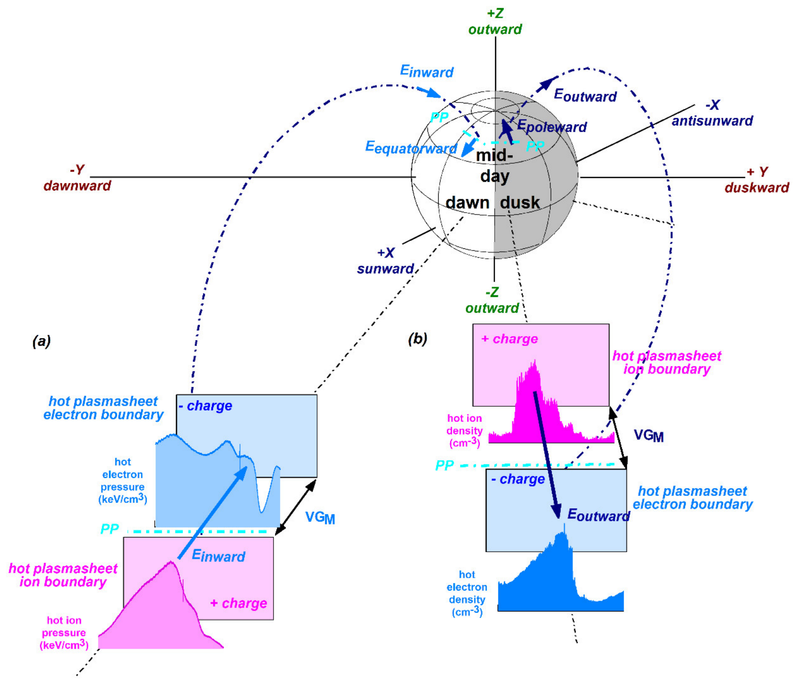
Figure 2.
The orbit maps depict the orbit sections of interest completed by THEMIS (in colors) and GEOTAIL (in blue) in (a) Event-1, (b) Event-2, (c) Event-3 and (d) Event-4.
Figure 2.
The orbit maps depict the orbit sections of interest completed by THEMIS (in colors) and GEOTAIL (in blue) in (a) Event-1, (b) Event-2, (c) Event-3 and (d) Event-4.
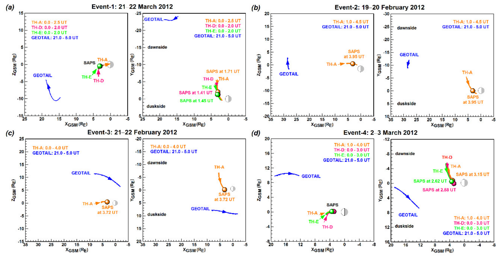
Figure 3.
The solar and geomagnetic conditions underlying (a) Event-1, (b) Event-2, (c) Event-3 and (d) Event-4.
Figure 3.
The solar and geomagnetic conditions underlying (a) Event-1, (b) Event-2, (c) Event-3 and (d) Event-4.
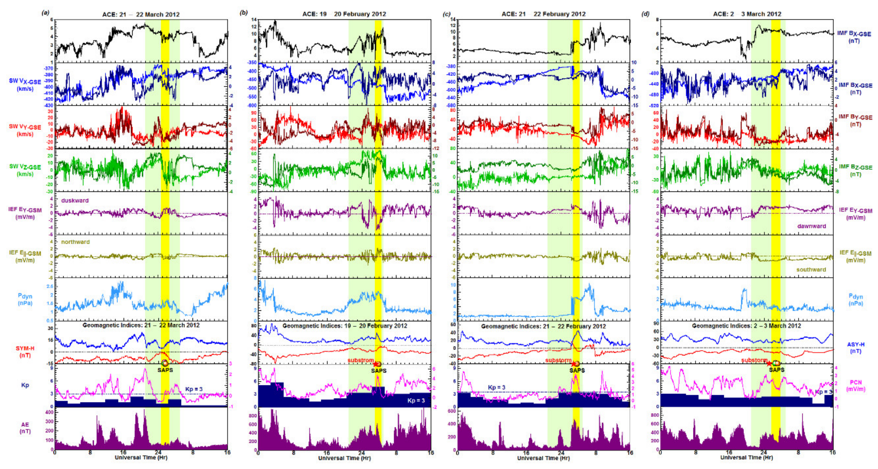
Figure 4.
Underlying Alfvenic plasmasheet conditions depicted by the line plots and by the scatter plots’ linear correlations and positive gradients in (a) Event-1, (b) Event-2, (c) Event-3 and (d) Event-4.
Figure 4.
Underlying Alfvenic plasmasheet conditions depicted by the line plots and by the scatter plots’ linear correlations and positive gradients in (a) Event-1, (b) Event-2, (c) Event-3 and (d) Event-4.
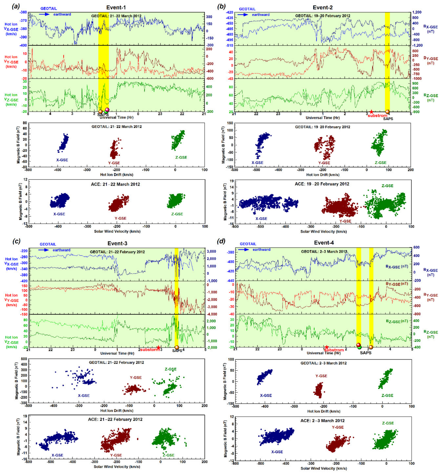
Figure 5.
The line plots depict (top panel) the underlying dispersionless particle injections, earthward directed hot ion surges (middle panel) and solar-wind dynamic pressure variations occurring in (a) Event-1, (b) Event-2, (c) Event-3 and (d) Event-4.
Figure 5.
The line plots depict (top panel) the underlying dispersionless particle injections, earthward directed hot ion surges (middle panel) and solar-wind dynamic pressure variations occurring in (a) Event-1, (b) Event-2, (c) Event-3 and (d) Event-4.
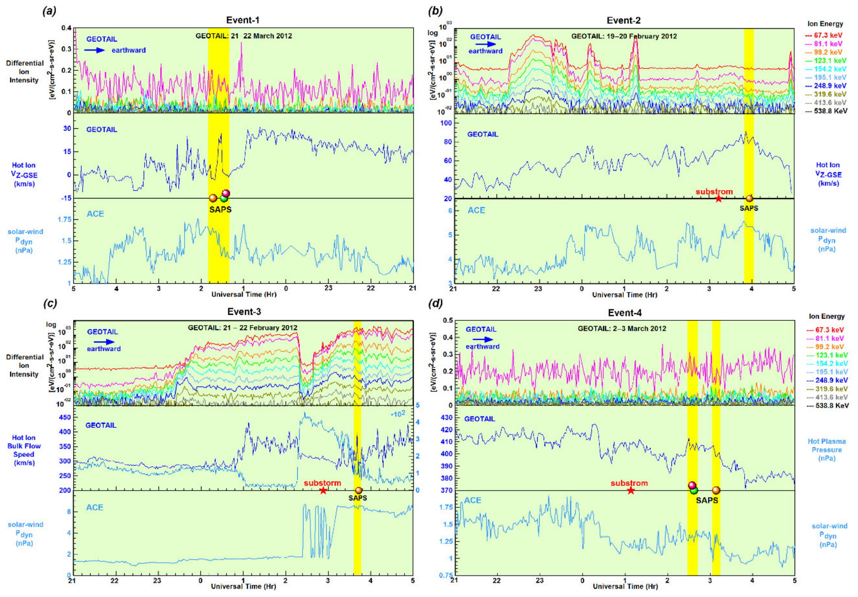
Figure 6.
The northern-hemisphere TEC map and TEC polar plot series illustrate the TEC distribution in (a) Event-1, (b) Event-2, (c) Event-3 and (d) Event-4.
Figure 6.
The northern-hemisphere TEC map and TEC polar plot series illustrate the TEC distribution in (a) Event-1, (b) Event-2, (c) Event-3 and (d) Event-4.
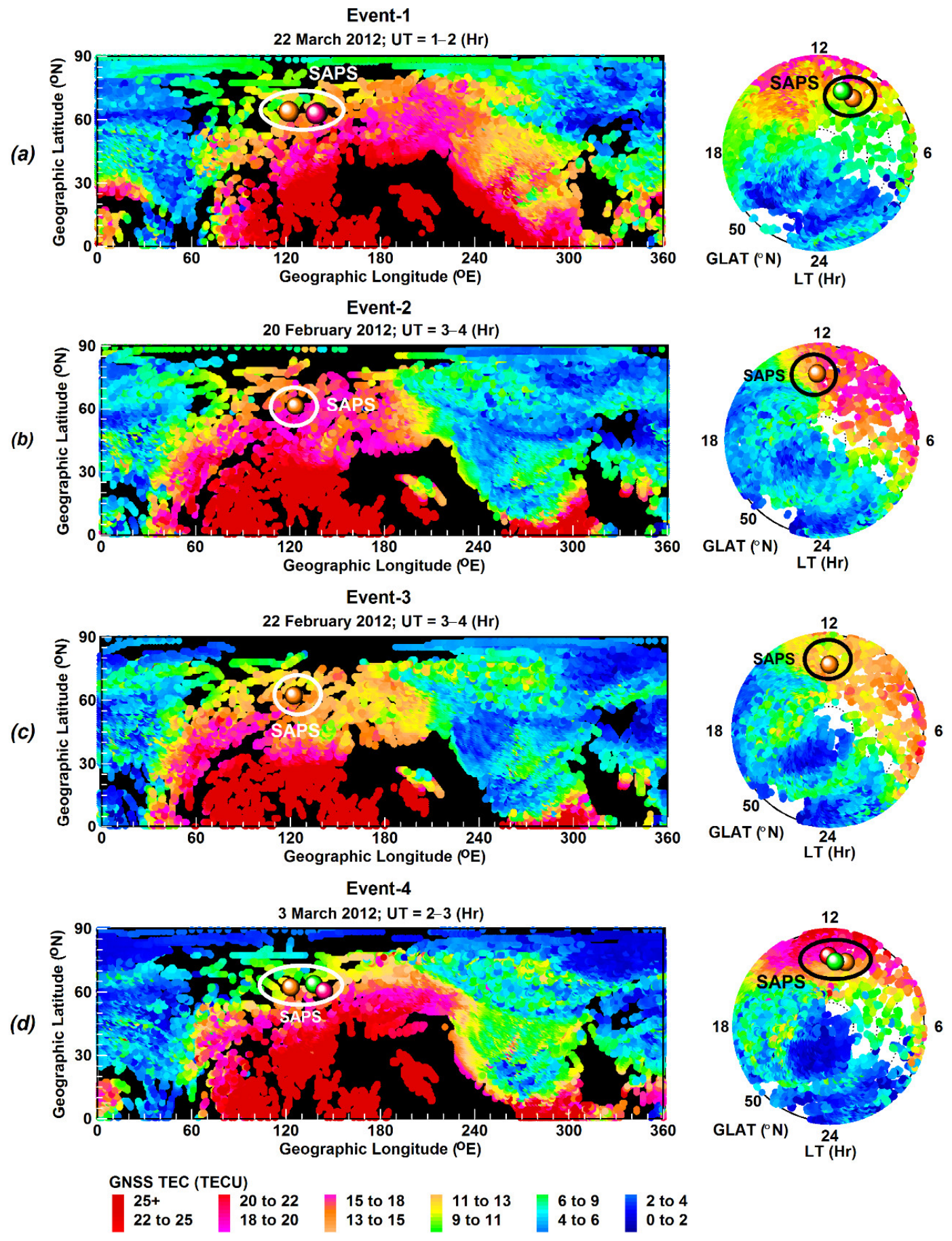
Figure 9.
Constructed for Event-4, the line-plot sets depict (a–c) the inner-magnetosphere SAPS channel and its plasma environment and (d) the whistler-mode waves developed.
Figure 9.
Constructed for Event-4, the line-plot sets depict (a–c) the inner-magnetosphere SAPS channel and its plasma environment and (d) the whistler-mode waves developed.
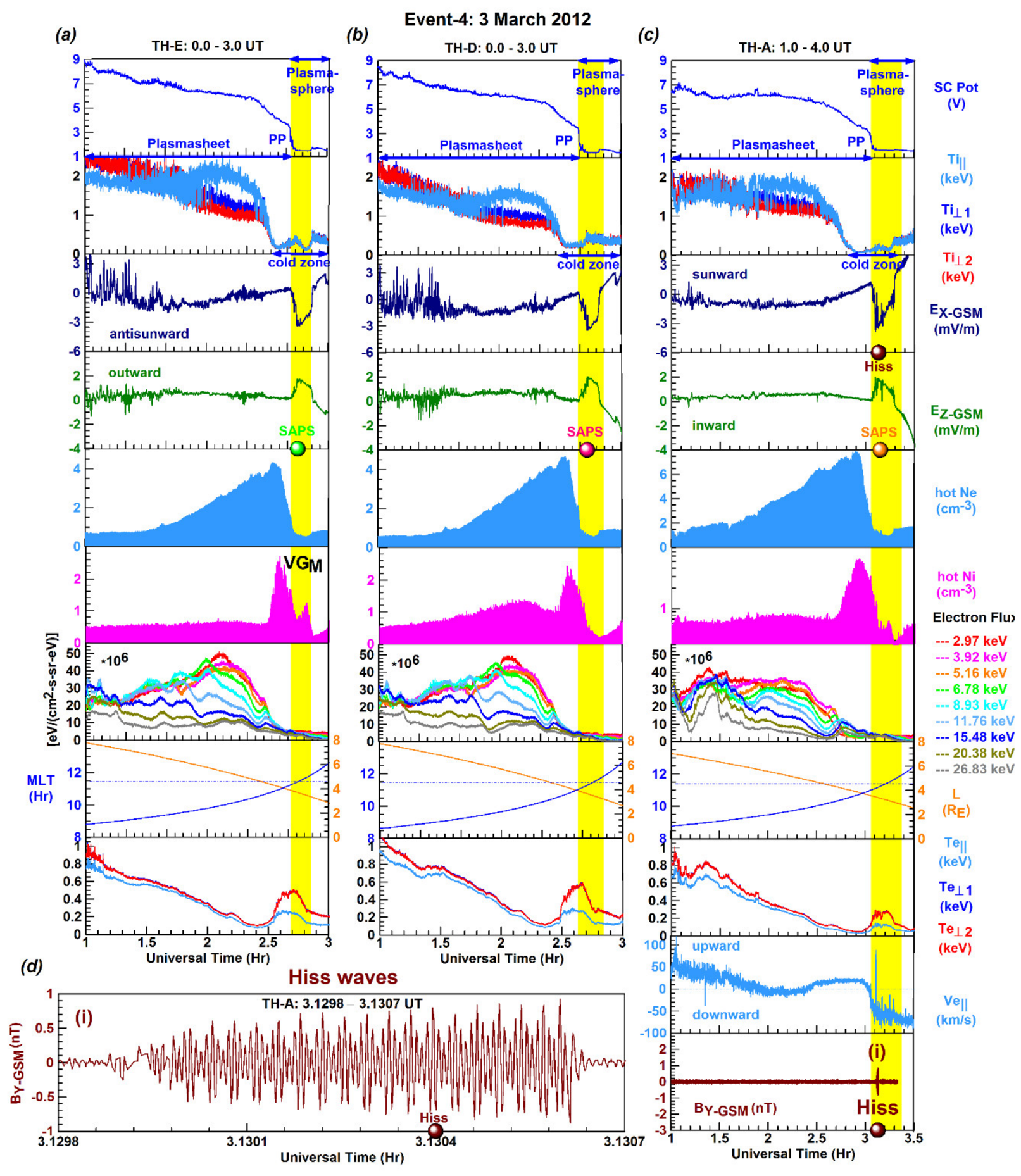
Figure 10.
Constructed for the 3 March 2012 SAPS events observed by THEMIS and DMSP F16, (a) the northern hemisphere map depicts the satellite footprints of THEMIS (in colors) and F16 (in cyan) along with the mapped-down flow channels (symbols in colors), (b) the TEC distribution over the northern hemisphere, and (c) the F16 line-plot sets illustrating the postnoon SAPS flow’s plasma environment.
Figure 10.
Constructed for the 3 March 2012 SAPS events observed by THEMIS and DMSP F16, (a) the northern hemisphere map depicts the satellite footprints of THEMIS (in colors) and F16 (in cyan) along with the mapped-down flow channels (symbols in colors), (b) the TEC distribution over the northern hemisphere, and (c) the F16 line-plot sets illustrating the postnoon SAPS flow’s plasma environment.
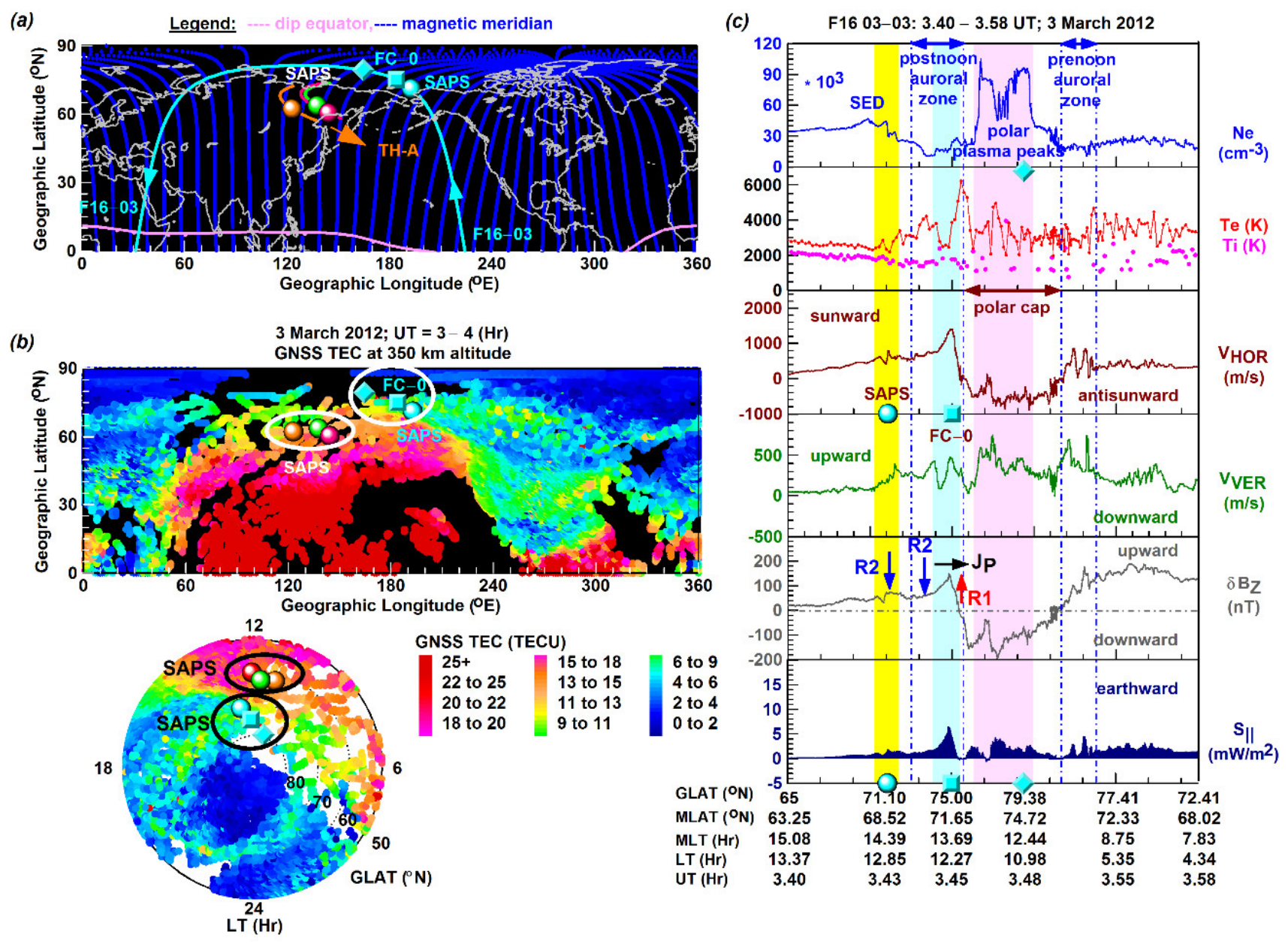
Figure 11.
Constructed for the 3 March 2012 prenoon SAPS event observed by DMSP F16, (a) the northern hemisphere map depicts the satellite footprints of F16 (in cyan) along with the mapped-down flow channels (symbols in cyan), (b) the TEC distribution over the northern hemisphere, and (c) the F16 line-plot sets illustrating the prenoon (LT) SAPS channel’s plasma environment.
Figure 11.
Constructed for the 3 March 2012 prenoon SAPS event observed by DMSP F16, (a) the northern hemisphere map depicts the satellite footprints of F16 (in cyan) along with the mapped-down flow channels (symbols in cyan), (b) the TEC distribution over the northern hemisphere, and (c) the F16 line-plot sets illustrating the prenoon (LT) SAPS channel’s plasma environment.
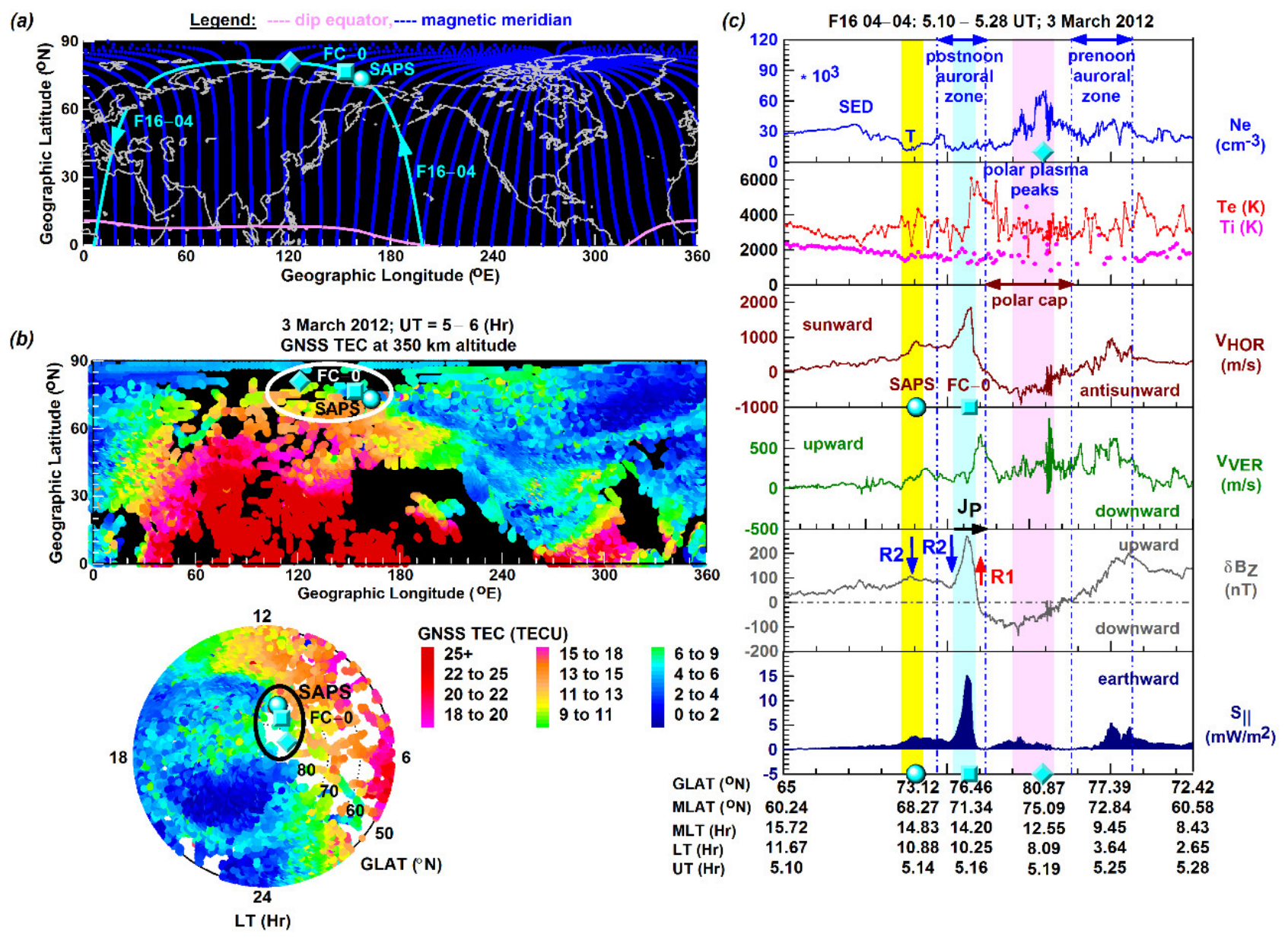
Figure 12.
Constructed for the 20 February 2012 midday SAPS event, the AMPERE δBFIT vector polar plot illustrates the midday WEJ scenario underlying the development of midday SAPS in the ionosphere.
Figure 12.
Constructed for the 20 February 2012 midday SAPS event, the AMPERE δBFIT vector polar plot illustrates the midday WEJ scenario underlying the development of midday SAPS in the ionosphere.
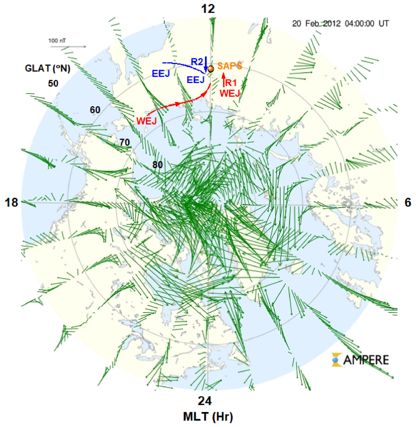
Figure 13.
Constructed for the 22 March 2012 prenoon SAPS event, the AMPERE δBFIT vector polar plot illustrates the EEJ scenario underlying the development of prenoon SAPS in the ionosphere.
Figure 13.
Constructed for the 22 March 2012 prenoon SAPS event, the AMPERE δBFIT vector polar plot illustrates the EEJ scenario underlying the development of prenoon SAPS in the ionosphere.
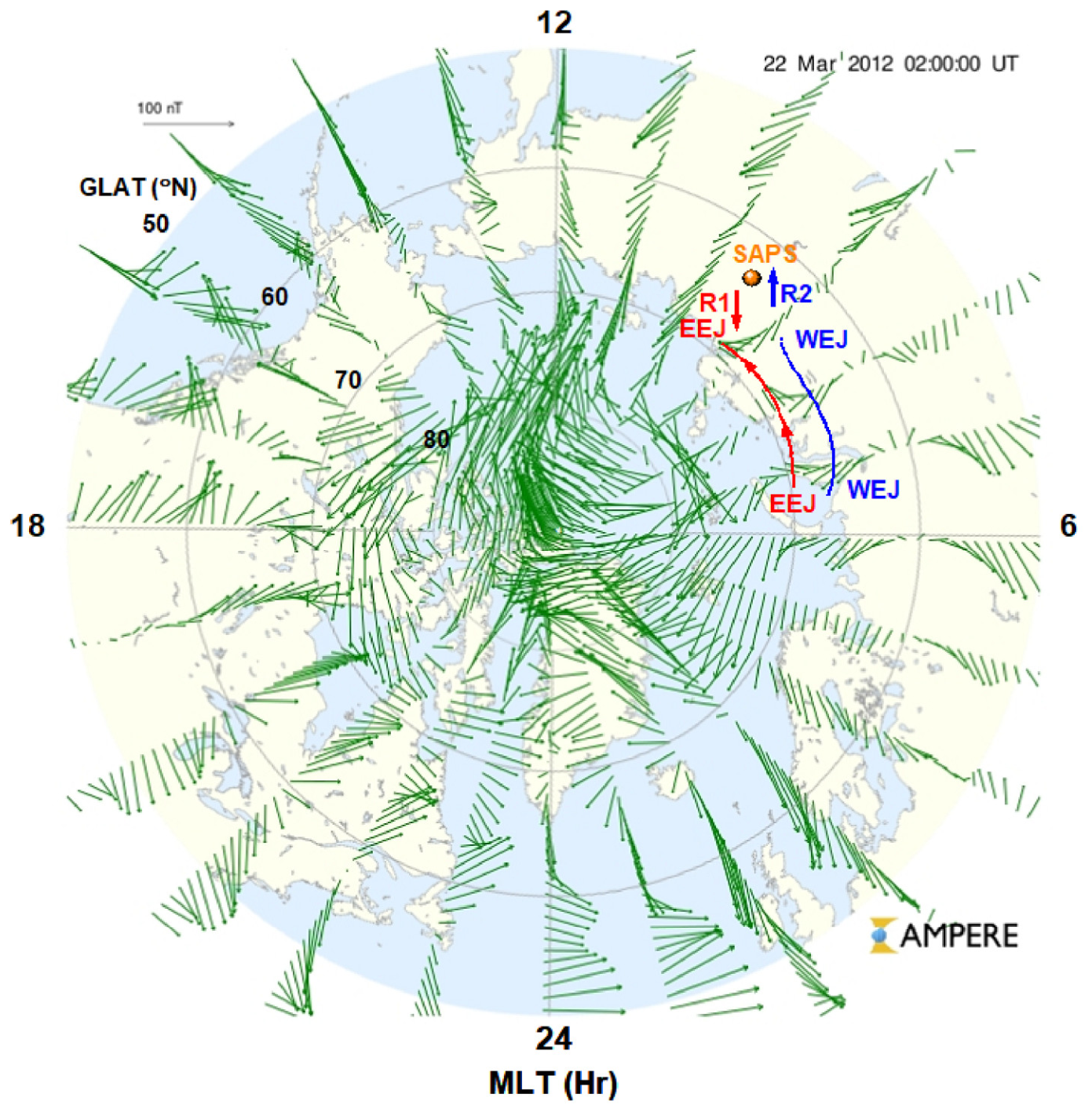
Disclaimer/Publisher’s Note: The statements, opinions and data contained in all publications are solely those of the individual author(s) and contributor(s) and not of MDPI and/or the editor(s). MDPI and/or the editor(s) disclaim responsibility for any injury to people or property resulting from any ideas, methods, instructions or products referred to in the content. |
© 2026 by the authors. Licensee MDPI, Basel, Switzerland. This article is an open access article distributed under the terms and conditions of the Creative Commons Attribution (CC BY) license (http://creativecommons.org/licenses/by/4.0/).
Copyright: This open access article is published under a Creative Commons CC BY 4.0 license, which permit the free download, distribution, and reuse, provided that the author and preprint are cited in any reuse.