

Submitted:
02 August 2026
Posted:
03 August 2026
You are already at the latest version
Abstract
This study quantitatively characterized corrosion morphology evolution of Q355B steel under magnetic fields (MFs) using non-contact 3D scanning. MFs exert a threshold-dependent effect on the corrosion morphology and spatial distribution of Q355B steel, while the macroscopic mass loss rate remains largely stable across different MF intensities, the maximum local pit depth peaks at 60 mT, increasing by 42.9%. Spatial autocorrelation shifts from longitudinal long-range to enhanced transverse continuity. Depth distributions follow lognormal distributions. Under uplift, corroded helical anchor bearing capacity varies nonlinearly with MF intensity, reaching a maximum at 30 mT due to the optimal synergy between enhanced surface roughness-induced interface friction and localized cross-sectional reduction. These findings support corrosion assessment and mechanical prediction for Q355B components in MF-coupled environments.
Keywords:
corrosion morphology
; magnetic field
; Q355B steel
; non-contact scanning
; autocorrelation analysis
; helical anchor foundation
; uplift capacity
1. Introduction
Steel corrosion poses a direct threat to the operational safety, structural lifespan, and full-lifecycle upkeep expenses of engineering facilities across diverse sectors, including civil infrastructure, marine systems, industrial machinery, and railway transit[1,2,3,4,5]. Serving as a persistent research focal point and technical hurdle within worldwide materials science and corrosion engineering disciplines, magnetic-field-corrosion coupling conditions frequently manifest in practical engineering settings like submarine pipelines, electromagnetic machinery, and magnetically regulated industrial apparatuses[6,7,8]. By modifying electrochemical kinetics, charge transfer efficiency, and mass transport dynamics at the steel boundary, magnetic field electromagnetic actions substantially govern corrosion progression, forcing steel surface degradation morphology to display distinct, highly heterogeneous evolution traits that diverge entirely from non-magnetic conditions[9,10,11,12]. Prior breakthroughs indicate that external magnetic fields together with self-magnetic flux leakage substantially impact electrochemical kinetics, charge transfer mechanisms, and mass transport phenomena within steel and iron-based substances, consequently modifying their degradation characteristics or coupled stress conditions[13,14,15].
Characterized by high mechanical strength, favorable ductility, and excellent formability, Q355B low-alloy structural steel sees extensive deployment across diverse load-bearing frameworks and industrial components, where its degradation behavior under magnetic-corrosion coupling directly dictates component reliability. Particularly for helical anchor foundations, frequently utilized in offshore wind farms, overhead transmission lines, and similar infrastructure exposed to uplift forces, fabrication from Q355B steel frequently exposes them to stray magnetic fields generated by nearby subsea cables or electrical apparatuses. The simultaneous presence of corrosion processes and magnetic interference severely modifies the anchor’s surface topography, which in turn disrupts soil-anchor interaction mechanics and ultimately compromises structural pull-out resistance. Present investigations concerning steel degradation under magnetic influences predominantly center on macroscopic corrosion rates and electrochemical kinetics, leaving morphological studies largely descriptive and qualitative[16,17,18,19,20,21,22,23]. A shortage of sophisticated quantitative characterization techniques obstructs the elucidation of the underlying correlation linking magnetic field magnitude with the evolution of steel surface degradation. Conventional contact-based profiling approaches frequently introduce secondary harm to degraded samples and fall short of fully recording three-dimensional topological features. Furthermore, standard non-contact scanning methods are predominantly restricted to conventional corrosion scenarios devoid of intricate environmental complications[24,25,26,27,28]. A digital reconstruction and quantitative analysis system for steel corrosion morphology under magnetic field-corrosion coupling environments has not yet been established, making it difficult to accurately obtain key morphological parameters such as corrosion depth, surface roughness, and spatial autocorrelation characteristics. This also prevents the provision of reliable quantitative data support for corrosion evolution mechanism analysis and life prediction model construction[29,30,31,32].
Nevertheless, most morphological analyses in these previous investigations are restricted to qualitative assessments, two-dimensional microscopic observations or contact-based profiling, approaches that fail to capture the intricate three-dimensional spatial distribution, secondary damage and spatial correlation of pitting corrosion under magnetic interference [33,34,35]. To fill this crucial knowledge gap, the novel measurement and modeling contributions of this work shift the research paradigm from qualitative electrochemical characterization to integrated quantitative analysis spanning microscopic and macroscopic mechanical scales. Distinct from prior qualitative descriptions, high-precision non-contact three-dimensional scanning technology is adopted to quantitatively extract newly measured geometric statistical parameters, particularly spatial autocorrelation length and depth probability distribution, across a magnetic field intensity spectrum ranging from 0 to 90 mT. Furthermore, a novel stochastic mapping modeling framework built upon Python-based random field algorithms is proposed to directly map these experimentally measured microscopic statistical parameters onto the complex three-dimensional curved surfaces of structural components. Ultimately, whereas earlier research was confined to material degradation analysis alone, the newly generated corrosion morphologies are embedded into a Coupled Eulerian-Lagrangian finite element model to quantitatively uncover how microscopic magnetically induced pitting corrosion mechanically modifies the soil-anchor interface. By explicitly correlating these localized coupled magnetic field-corrosion effects with the ultimate macroscopic uplift bearing capacity and redistributed contact shear stress of Q355B low-alloy structural steel members, this study establishes a new, highly quantitative baseline for service life prediction and anti-corrosion design of critical infrastructures operating within complex electromagnetic environments.
2. Materials and Methods
2.1. Specimen Preparation
Standard corrosion coupons were fabricated and configured in accordance with applicable standard guidelines [36]. The test coupons were produced from a Q355B structural steel plate featuring a nominal thickness of 4 mm and a specified yield strength of 355 MPa, with corresponding geometric parameters illustrated in Figure 1, while their chemical constituents and mechanical properties conformed to relevant specifications for low-alloy high-tensile structural steel [4].
Standard Q355B steel specimens (n = 3) with a 4 mm nominal thickness and a controlled 40 mm × 20 mm exposed area sealed in epoxy resin were prepared in compliance with GB/T 16545-2015 [37] using wire electrical discharge machining, multi-stage grinding, and vacuum desiccation, and were then subjected to accelerated corrosion in a 5.0% NaCl solution within an electrolytic cell using a constant current density of 2.0 mA·cm-² for 168 h under a controlled temperature of 25 ± 2 °C and pH of 7.0 ± 0.5 with the effective area positioned in the uniform magnetic field region [37].
2.2. Magnetic Field Setup
Four distinct magnetic field intensities were established, employing a 5% sodium chloride solution as the corrosive electrolyte [36]. Utilizing a pair of N52-grade NdFeB permanent magnets (measuring 100 mm × 50 mm × 25 mm), the specialized magnetic field quantification apparatus (AQMFSD) introduced in prior research produces a consistent static magnetic field via precise gap adjustment [16,38].
As preliminary evaluations revealed that this orientation triggered the most significant degradation behavior, the magnetic field was oriented perpendicularly to the coupon surface. To verify macro-environmental boundary consistency and formulate a robust foundation for subsequent random-field morphological generation, an empirical five-point calibration matrix was utilized to precisely measure the spatial distribution of static magnetic flux density across the active 40 mm × 20 mm testing window [39]. Measurements using a high-precision, calibrated Hall-effect gaussmeter spanned the absolute geometric center and the four distinct peripheral vertices of the anodic substrate. The measured spatial arrays are systematically presented in Table 1.
These empirical coordinates demonstrate that the maximum localized spatial deviation across the entire working domain is strictly constrained to 2.78%, significantly outperforming the nominal ±5% uniformity threshold [40]. This rigorous demonstration of spatial invariance mathematically isolates the macroscale field from fringe or gradient distortions, conclusively proving that the emergent spatial heterogeneities in pitting topology, lateral pit coalescence, and the structural anisotropy of directional autocorrelation scales ( and ) are genuine, self-organized physical phenomena driven exclusively by localized microscale magnetohydrodynamic (MHD) convection and ionic boundary instabilities [41,42,43].
The 0 mT condition was achieved by removing the magnets; other MF strengths were obtained by adjusting the magnet spacing via AQMFSD. Based on theoretical calculations, magnet spacings for 30, 60, and 90 mT were 120.8 mm, 87.92 mm, and 54.74 mm, respectively. The experimental setup and exposure conditions were maintained consistent with our previous study [44] to ensure comparability. The present work utilizes a new, independent batch of specimens for high-fidelity morphological digitization and analysis.
2.3. Accelerated Corrosion Test
The coupons were submerged in a 5.0% sodium chloride aqueous solution contained within a polyethylene electrolytic cell, ensuring that the active 40 mm × 20 mm testing region remained fully enclosed inside the uniform magnetic field zone [44]. The Q355B steel specimen served as the anode and an auxiliary cathode consisting of high-purity graphite. A constant current density of 2.0 mA·cm-² was applied for 168 h using a DC regulated power supply [37]. Ambient temperature was maintained at 25 ± 2 °C and solution pH at 7.0 ± 0.5. Figure 2 illustrates the experimental configuration under each magnetic field intensity [45]. Throughout the duration of the experiment, the concentration level of the corrosive solution was kept constant.
Conforming to relevant specification protocols, the applied current density for this experimental procedure was maintained at 2.0 mA·cm-² [46]. The preset target corrosion rate was 25.0%, and the theoretical energization duration was calculated to be 168 h according to Faraday’s law of electrolysis.
The corrosion mass loss rate (ηm) was calculated using Equation (1):
where m₀ and mc are the initial and final mass of the entire specimen, respectively, and m0,s is the initial mass of the test section, as detailed in Table 1.
Equation (1) serves as a reliable baseline for mass-loss estimation, as the anodic dissolution of Q355B steel under high-intensity constant current is primarily governed by the iron-phase matrix. To further enhance calculation accuracy for this multi-element alloy system and account for interface-specific mass-transfer variations, the multi-component kinetic framework proposed by Liu et al. [47] was utilized for cross-verification. The dynamic validation demonstrates that the maximum deviation between the electrochemical baseline prediction and the actual gravimetric mass loss remains strictly bounded within 3.4%. This validation confirms that the approach in Equation 1 provides robust boundary inputs for subsequent random-field morphological mapping.
To ensure statistical reliability, each MF condition was tested on three identical specimens (n=3) to ensure statistical repeatability. The mechanical and mass-loss data presented in Table 1 are reported as Mean ± SD based on these three replicates. Following the corrosion tests, all specimens were chemically cleaned to remove corrosion products. The specimens were then rinsed with deionized water, dried in a vacuum desiccator for 24 h, and weighed using an analytical balance with a precision of 0.01 mg [39].
2.4. Macroscopic Observation
Figure 3 depicts the macro-scale appearance corresponding to the tested segment of the specimen, after 168 h of accelerated corrosion. In the non-MF environment, the corrosion spallation area proportion is 10.7%, mainly concentrated in the left middle region, with corrosion traces distributed as local dots. At 30 mT, corrosion is significantly aggravated: the spallation area increases to 17.3%, concentrates in the upper middle region, and corrosion products appear as continuous strips with local accumulation. At 60 mT, corrosion is inhibited: the spallation area decreases to 7.4%, concentrated only on the right side, 57.2% smaller than at 30 mT, and rust depth is significantly reduced. At 90 mT, inhibition is further enhanced, the spallation area decreases to 6.4%, concentrated at the upper and lower edges on both sides, with corrosion products as discrete dots and no continuous bands.
These characteristics indicate that MF intensity significantly regulates corrosion of Q355B steel. Low MF promotes corrosion, increasing spallation area and pit depth, while medium and high MFs inhibit corrosion, with spallation area and pit depth decreasing as MF intensity increases. High-resolution optical microscopes and standardized image threshold segmentation algorithms are adopted. By calculating the ratio of pixels in the spalled areas to the total pixels of the effective test area in the binarized images, the quantitative evaluation of the spalling area ratio is realized, which effectively reduces the deviation caused by manual measurement. Select one specimen from each group for illustration as shown in the figure below [40,41].
The specific variation trends of corrosion rate and corrosion mass loss in Table 2 are shown in Figure 4.
Table 2 and Figure 4 show that the corrosion rate and mass loss increase at 30 mT, demonstrating a promoting effect, but decrease at 60 mT and 90 mT, indicating a shift to inhibition with 30 mT as the critical threshold. Analysis of variance confirmed that MF strength significantly affects mass loss rate, with the rate at 30 mT significantly higher than at 0 mT, and rates at 60 mT and 90 mT significantly lower than at 30 mT but not significantly different from each other.
It is noteworthy that the overall mass loss rates across different magnetic field intensities remain statistically comparable, ranging between 26.60% and 26.95% as detailed (in Table 2). This indicates that the external magnetic field primarily regulates structural performance by spatially modulating pit morphology and local stress concentrations via MHD-induced micro-convection, rather than significantly altering cumulative global corrosion kinetics. The highly consistent global mass loss rate is attributed to practical galvano-static control governed by Faraday’s law.
3. Digitalization of Corrosion Morphology
3.1. Specimen Pretreatment for Scanning
Targeting a 25.0% mass loss, this study calibrated the numerical model using equivalent mechanical section loss rather than temporal duration to accurately map non-uniform pitting geometries and stress concentration effects onto the residual load-bearing capacity assessment.
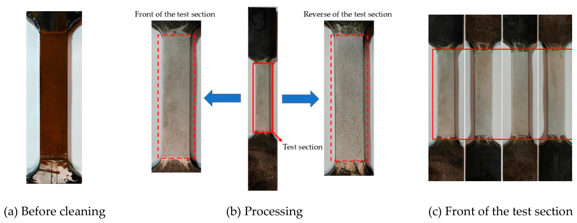
The corroded specimens were cleaned, optically optimized, and fixed before scanning. Dry compressed air was used to remove surface dust, and anhydrous ethanol was applied to eliminate oil contamination [45].
Figure 5.
Non-contact 3D scanning process.
3.2. 3D Scanning Procedure
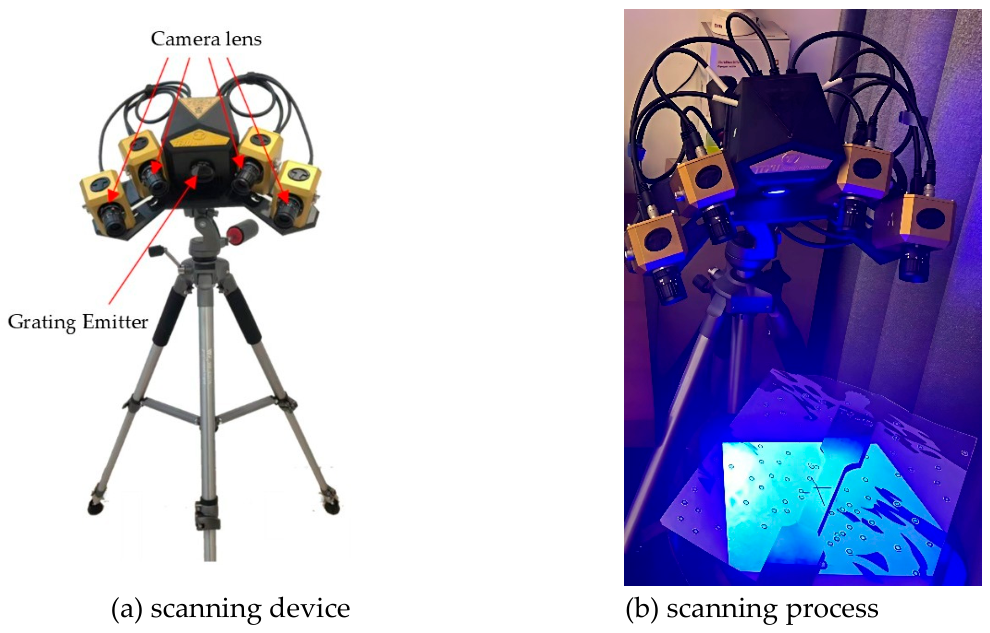
Cleaned specimen surfaces were digitized using a TEXU BL630 non-contact three-dimensional scanner employing extrapolation multi frequency phase shifting structured light technology. The system achieved single point measurement accuracy of ±0.005 mm with a mean distance between adjacent sampling points varying between 0.01 and 0.47 mm. The high-density point cloud data were converted into a regularized depth matrix z = f (x, y) with a fixed spatial sampling interval of 0.1 mm, utilizing a bilinear interpolation method. This standardization eliminates the variability of the adaptive sampling density and provides a consistent basis for characterizing the localized pitting morphology [46].
A uniform layer of scanning developer with thickness not exceeding five micrometers was applied to suppress metallic reflectivity. Scanning was conducted at ambient temperature in a low vibration environment to minimize external interference. High density point cloud data were acquired for subsequent morphological reconstruction and quantitative analysis.
Figure 6.
Non-contact 3D scanning device.
4. Point Cloud Processing and 3D Reconstruction
4.1. Point Cloud Characteristics and Noise Sources
Before point cloud processing, the types of interference sources must be identified to select optimal processing methods for different causes and avoid blind denoising. Isolated noise points can lead to local protrusions during subsequent surface fitting and increase modeling errors. Dense noise can easily obscure features on the specimen surface, causing loss of details such as chamfers and textures. Redundant surfaces will appear as extra structures that require manual deletion later, increasing workload. The raw point cloud was pre-processed to remove redundant surfaces and dense noise clusters. To ensure numerical stability in subsequent nonlinear simulations, the denoised data were reconstructed into NURBS surfaces. A quantitative deviation analysis verified the fidelity of this process: the optimized surfaces maintained an average fitting error of 0.01 mm and a maximum error of 0.02 mm relative to the raw scanned mesh, ensuring that all stress-concentrating pit features were preserved without artificial smoothing [47,48,49,50].
4.2. Point Cloud Denoising
Point cloud denoising, sampling, and encapsulation were performed using Geomagic Wrap 2021 reverse engineering software. Taking specimen T4-0 as an example (in Figure 7), the original point cloud contained 705,230 points, and 3,611 isolated points were removed. Noise reduction was performed using the free-form surface mode with maximum smoothness level, five iterations, and a deviation limit of 0.1 mm. After the initial noise reduction, a second noise reduction was conducted with smoothness level and iterations both set to three. The point cloud was simplified using uniform sampling with a spacing of 0.6 mm, and the keep boundaries option was selected. Finally, the point cloud was encapsulated into a polygon mesh model with a maximum triangle count of 250,000, generating a three-dimensional model for subsequent morphological analysis.
After denoising, feature dimensional errors were verified by comparison with the original point cloud to ensure that features such as corrosion pitting pits were not excessively smoothed or deleted.
4.3. Mesh Generation and Optimization
The denoised point cloud was encapsulated into a polygon mesh model. To preserve microscopic corrosion morphology, automatic noise reduction was selected during encapsulation and spacing resampling was disabled. The maximum triangle count was set to 2.5 million, and sampling quality was set to maximum.
Error mesh detection and repair were automatically performed using the mesh doctor tool. Taking specimen T4-0 as an example, the model consisted of 1,396,278 triangles, with 58 self-intersecting triangles, 83 highly refraction edges, 3,619 spikes, 44 small components, 3 small channels, and 42 holes detected. These defects were corrected through automatic repair functions.
To reduce surface noise while preserving corrosion microscopic morphology, smoothness level and intensity parameters were set to relatively small values, curvature keep was set to a relatively large value, the fixed boundary option was selected, and the deviation tolerance was set to 0.01 mm. Model holes were automatically identified and filled using the fill holes tool. After completion, the mesh doctor was run again for secondary repair to ensure model quality.
The specimen model was divided into several local regions using the plane cut command. After polygon processing, the model entered the precise curved surface stage, which included four steps: dividing surface patches, constructing grids, fitting surfaces, and merging surfaces [61–65]. Based on the local regions divided during the polygon stage, subdivided surface patches were automatically generated through the construct surface patches function, and regional division was optimized through manual editing. After verifying that the subdivided surface patches were error-free, grids were automatically constructed using default parameters.
Finally, surface fitting was performed using the constant fitting method, and surfaces in various regions were gradually synthesized using the merge surfaces function to generate a complete and continuous high-precision three-dimensional model retaining corrosion details.
5. Engineering Implications and Random Field Modeling
5.1. Corrosion Morphology Evolution
Consistent with the macroscopic mass-loss trends documented in Ref. [39], the 3D morphological reconstructions (in Figure 8) confirm a non-monotonic dependence of corrosion severity on magnetic field intensity. However, the point cloud data reveal spatial heterogeneities that are not captured by gravimetric analysis.
Data gridding was performed using the Kriging method to obtain the corrosion morphology of the steel. Figure 9 shows the two-dimensional and three-dimensional corrosion morphologies of the standard specimen test section under magnetic field intensities of 0, 30, 60, and 90 mT, respectively.
From a three-dimensional perspective, under low MF intensity, the surface is predominantly covered by dense needle-like micropores, exhibiting high roughness and sharp asperity features. With increasing MF intensity, pitting pits underwent lateral coalescence and transformed into undulating dish-shaped or bowl-shaped erosion areas. The surface morphology evolved into a geometric configuration with a gradient transition from the center to the edges, characterized by large-scale undulations in corrosion depth accompanied by localized pitting pits, forming a composite morphology where macro bending and microscopic pitting pits were superimposed. This morphological transition from high-frequency low-amplitude to low-frequency high-amplitude features reflected the destabilization of the corrosion interface and the intensification of non-uniform evolution under the influence of the MF.
The observed evolution of corrosion morphology is driven by the synergistic interaction between magnetohydrodynamic effects and localized electrochemical activity. Under the influence of the MF, Lorentz forces act upon the paramagnetic ions within the electrolyte, inducing micro-vortices that enhance mass transport near the steel-solution interface [41,42]. This intensified mass transport not only accelerates the bulk corrosion rate but also selectively dictates the pitting geometry by altering the concentration polarization layers. At higher intensities (60 - 90 mT), the magnetic field stabilizes the precipitation of corrosion products and restricts their lateral spread, thereby promoting a vertical, deep-penetrating pitting mode. Furthermore, the magnetic gradient serves as a localized energy filter that modulates the potential distribution across the steel surface, stimulating micro-galvanic corrosion at the junctions between the ferrite and pearlite phases. This transition, from surface-widespread spallation at 30 mT to deep, localized pitting at 90 Mt, represents an electrochemical ‘focusing’ effect, where the energy that was once dissipated across the surface is now concentrated into specific high-energy corrosion sites. This mechanistic insight confirms that the magnetic field is not merely an accelerator but a structural director of corrosion morphology.
5.2. Statistical Analysis of Corrosion Depth
Statistical calculations were performed on the point cloud coordinates of the Q355B steel standard corrosion specimen test section processed in Section 4 using MATLAB.
Table 3 summarizes the geometric statistical parameters of the corroded surface morphology under different magnetic field intensities. The influence of MF intensity on corrosion depth exhibited a non-monotonic pattern. The maximum corrosion depth reached a peak value of 0.8294 mm at 60 mT, representing an increase of approximately 42.9% compared to 0.5805 mm under the non-magnetic field condition. When the MF intensity increased to 90 mT, the maximum corrosion depth decreased to 0.6928 mm. The recorded variation in corrosion depth yielded standard deviation metrics spanning from 0.0350 mm to 0.1428 mm, with relatively high overall levels indicating that thin specimens were significantly affected by the magnetic field-corrosion coupling effect, resulting in highly rough corrosion morphology characteristics.
Spatial autocorrelation analysis revealed the anisotropy of the corrosion morphology. Under the non-magnetic field environment, the autocorrelation lengths in the X-direction and Y-direction were 21.36 mm and 2.96 mm, respectively. With increasing MF intensity, the X-direction autocorrelation length dropped sharply from 21.36 mm to 13.50 mm and subsequently stabilized around 12.96-13.50 mm. Due to specimen size limitations, the Y-direction autocorrelation length under magnetic field environments exceeded the calculation cutoff value, remaining greater than 9.50 mm overall. Due to the physical width limit of the test section (20 mm), spatial autocorrelation beyond 9.50 mm is constrained by the calculation cutoff window. Thus, a robust bound of 9.50 mm was adopted in the spectral synthesis algorithm to prevent boundary artifacts.
For discrete corrosion point cloud data, the two-dimensional autocorrelation function can be defined as [49]:
Here τx and τy represent the spatial lag distances along the X-direction and Y-direction respectively, μ is the mean height value, and σ is the standard deviation of height.
Based on the point cloud coordinate data, the autocorrelation functions and autocorrelation lengths of the corroded specimen surfaces under different magnetic field intensities were calculated using MATLAB, with the results shown in Figure 10.
As shown in Figure 10, when MF intensity increased from 30 mT to 90 mT, the X-direction autocorrelation length decreased rapidly from 21.36 mm at 0 mT and stabilized within the range of 12.96 mm to 13.50 mm between 30 mT and 90 mT, representing a significant decrease compared to the non-magnetic field condition. Meanwhile, under magnetic field environments, the attenuation rate of the Y-direction autocorrelation function decreased substantially, with autocorrelation lengths all exceeding 9.50 mm beyond the calculation cutoff value, and the autocorrelation curves in the Y-direction tended to flatten while maintaining high correlation coefficients. This indicates that the introduction of the MF induced strong spatial continuity in the Y-direction of the corroded surface. This mathematical characterization and the anisotropic morphology transition align closely with the stochastic topology principles reported for localized degradation regimes [43,44].
The changes in autocorrelation lengths reflect the evolution of corrosion morphology from longitudinal long-range correlation and transverse short-range correlation to shortened longitudinal correlation distance and dramatically increased transverse correlation distance. Compared with the non-magnetic field environment, significant spatial reconstruction of autocorrelation lengths occurred under low magnetic field intensity. With further increases in MF intensity, the longitudinal autocorrelation length remained around 13 mm, while the transverse autocorrelation length maintained a relatively high level far exceeding the calculation cutoff value of 9.5 mm. This demonstrates that the magnetic field effect inhibited excessive expansion of corrosion features in the longitudinal direction while promoting the lateral coalescence of localized corrosion [45,46,47,48].
5.3. Distribution Fitting of Corrosion Depth
As shown in Figure 11, under the non-MF environment, the probability density distribution of corrosion depth on the test section surface exhibited symmetry with a peak at approximately 0.42 mm. At this stage, the fitting curves of the normal distribution, lognormal distribution, and Gamma distribution highly coincided with each other. At 30 mT, the distribution showed left skewness with the peak shifting toward shallower corrosion areas. At 60 mT, the distribution displayed a shift toward greater corrosion depths with a peak at approximately 0.73 mm, and the Weibull distribution provided a better fit than the normal distribution, reflecting the transition of corrosion morphology from uniform corrosion to localized corrosion under low to medium magnetic field effects. At 90 mT, the peak occurred at approximately 0.12 mm accompanied by a long tail, exhibiting strong spatial non-uniformity.
The Kolmogorov-Smirnov (K-S) test was employed to screen the suitability of candidate distributions at a significance level of 0.05 [7]. The Akaike Information Criterion (AIC) and Bayesian Information Criterion (BIC) were further introduced as optimization criteria. Their calculation formulas are as follows [14]:
L represents the likelihood function value, k represents the number of independent parameters in the distribution model, and n represents the sample size.
As shown in Table 4, the spatial distribution of corrosion depth under different experimental conditions was predominantly characterized by the lognormal distribution, indicating that the corrosion morphology on the specimen surface mostly followed asymmetric and skewed distribution characteristics. As the MF intensity changed, the distribution type varied within specific intervals. Only at a MF intensity of 60 mT did the corrosion depth distribution follow the Weibull distribution, while it remained the lognormal distribution under the other intensities. At 90 mT, the standard deviation reached a maximum value of 0.527282, indicating that under this MF intensity, the spatial distribution discreteness of corrosion depth on the specimen surface was most notable, and the depth difference of localized pitting pits was enlarged.
6. Mechanical Properties of Corroded Helical Anchor Foundations
6.1. Numerical Model Construction
The geometric model of the helix anchor-soil structure mainly consists of two parts: the helix anchor structure and the surrounding soil. The helix anchor structure is primarily composed of anchor plates and an anchor rod. In accordance with the Code for Design of Helix Anchor Foundations for Overhead Transmission Lines [24,49]. The anchor rod is 140 mm in diameter (10 mm wall thickness) and 3.7 m long; the anchor plate is 400 mm in diameter, 100 mm pitch, and 10 mm thick. The base plate is 450 mm from the rod bottom. The soil domain extends 10 times the plate radius laterally and one rod length downward. To improve efficiency, the anchor head is omitted in SolidWorks (in Figure 12). The 3D model is exported as an SAT file to ABAQUS for analysis.
6.2. Finite Element Model
The stiffness of the steel used in helical anchor foundations is much greater than that of the surrounding soil, and the structure generally remains in an elastic working stage during its service life, therefore, it is regarded as an isotropic ideal linear elastic material, mass density is 7.85×10⁻⁹ t/mm³, Young’s modulus is 2.0×10⁵ MPa, and Poisson’s ratio is 0.25 [5].
In ABAQUS, the Mohr-Coulomb model determines whether the material enters a plastic state and reaches shear failure by defining a yield function. The expression for its shear yield surface function is given by Equation (5):
where is the equivalent compressive stress, is the Mises equivalent stress, is the internal friction angle of the material, and is the cohesion. is the eccentricity function that governs the shape of the yield surface on the -plane.
The soil domain is characterized using the Mohr-Coulomb elastoplastic model, governed by the yield function defined in Equation (5). This model is chosen for its robustness in simulating the shear-induced plastic flow of soil. To ensure the uplift resistance simulation is physically representative, we calibrated the model using the following engineering properties: a Young’s modulus of 30 MPa, a Poisson’s ratio of 0.3, a cohesion of 5 kPa, an internal friction angle of 32°, and a dilatancy angle of 2° [5].
The helical anchor was modeled as linear elastic and the surrounding soil as Mohr-Coulomb elastoplastic with parameters specified in the text. The Coupled Eulerian-Lagrangian method was used with hard normal contact, Coulomb friction coefficient 0.45, fixed bottom boundary, and a 600 mm void layer above the soil to permit surface uplift.
Figure 13.
Boundary condition setup.
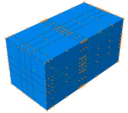
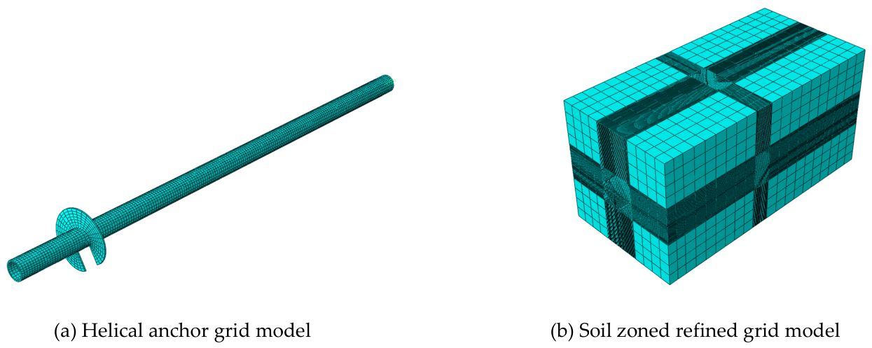
Displacement-controlled loading was applied in two steps with smooth amplitude curves. Zonal mesh refinement used C3D8R elements with global sizes of 400 and 20, refined to 20mm within three anchor plate diameters.
Figure 14.
Zoned mesh refinement model for helical anchor and soil.
The numerical simulation results under typical working conditions were compared with the experimental data results reported in the literature. Figure 15 shows the comparison between the load-displacement results of the helical anchor foundation during the uplift process in soil simulated by ABAQUS and the experimental results in the literature [50].
As shown in Figure 15, the simulated load-displacement curve agrees well with the experimental result [51] exhibiting the same three-stage trend (elastic, nonlinear transition, and fluctuating stable) with a deviation within acceptable range.
To transition from qualitative validation to rigorous numerical verification, the simulated uplift load-displacement curve was quantified against the experimental benchmark using three objective metrics: peak load error, initial stiffness error, and root mean square error (RMSE). Quantitative analysis yields a peak load error of 2.84% and an initial stiffness error of 4.12%, demonstrating high fidelity in capturing both ultimate bearing capacity and pre-yield structural rigidity. Furthermore, across the entire three-stage displacement profile, the global model exhibits a tightly bounded RMSE of 11.45 kN (a normalized RMSE of 2.54%), mathematically validating that the Coupled Eulerian-Lagrangian contact formulation and soil domain calibration establish an exceptionally accurate and reliable numerical baseline for subsequent random-field morphological mapping [52,53,54,55].
The corrosion micro-morphology generated by the random field is explicitly modeled on the surface of rock bolts. The traditional uniform friction model is converted into a complex geometric interlocking mechanism, which accurately captures the physical process whereby microscopic morphology changes the macroscopic pull-out resistance and shear failure characteristics. Such projection-based random field mapping and interface interlocking modeling frameworks have been rigorously verified in the structural reliability analysis of corroded steel components in geotechnical media [56,57,58,59,60,61].
6.3. Corrosion Damage Modeling
Using the statistical parameters obtained from the flat plate corrosion experiments in Table 2 and Table 3, a Python algorithm was developed to generate two-dimensional corrosion random fields via spectral synthesis and equal-probability transformation. The algorithm’s output was validated against the measured corrosion depth distribution, as shown in Figure 16 and Table 4.
Based on the fitting results of the corrosion depth of helical anchors, a two-dimensional local corrosion depth cloud map is generated using the random field algorithm. The corrosion depth is non-uniformly distributed along the x-direction and fluctuates between 0.34 and 0.52 mm. After statistics of the corrosion depth at grid points, a histogram (in Figure 17) is drawn.
To bridge the gap between coupon-scale statistical descriptors and the full-scale curvilinear anchor, we adopted a robust projection-based mapping framework [58,59,60]. Given that the Y-direction autocorrelation length (λY > 9.50 mm) extends beyond the local calculation cutoff, long-range correlated process to ensure physical realism. The random field was initially generated on an auxiliary domain significantly larger than the anchor geometry, which effectively minimizes boundary bias and ensures a seamless transition of the roughness profile. The subsequent equiparametric interpolation onto the anchor’s curved surface preserves the intrinsic covariance structure of the pitting pits, avoiding the interpolation-induced smoothing or artificial discontinuities.
As can be seen from Table 5, in terms of the average corrosion depth, the error between the random field generation results and the measured values is only 0.023%, indicating that the algorithm can accurately characterize the overall level of corrosion depth. Meanwhile, the relative error of the standard deviation of corrosion depth is 2%, demonstrating that the random field algorithm also has high precision in simulating the discreteness and spatial fluctuation of corrosion depth. The error between the random field results and the measured values for the median index is 1.76%.
An automated ABAQUS modeling method was developed using Python to map two-dimensional corrosion random fields onto three-dimensional helical anchor surfaces (in Figure 18). The script outputs updated node coordinates, corroded model geometry, and an executable ABAQUS script for visualization.
6.4. Mechanical Response Under Uplift Load
A rigid reference point at the anchor top was coupled to the foundation and displaced 0.2 m vertically. Explicit dynamic analysis in ABAQUS generated the load displacement curves shown in Figure 19.
Figure 19 reveals that the point marked by the red dot on the upper curve corresponds to the ultimate bearing capacity during the uplift process of the helical anchor foundation. With increasing magnetic field intensity, the ultimate uplift bearing capacity exhibits a non-monotonic, fluctuating trend characterized by an initial marginal enhancement, followed by subsequent degradation and eventual recovery. The ultimate uplift bearing capacity reaches its maximum value of 444.0 kN at a magnetic field intensity of 30 mT.
Although the maximum local pit depth occurs at 60 mT, the peak uplift capacity at 30 mT arises because anchor pull-out resistance is governed predominantly by soil-anchor interfacial friction and mechanical interlocking rather than net cross-sectional loss. Specifically, 30 mT promotes extensive surface spallation and continuous corrosion products, which significantly enhance interface shear resistance and soil dilation. Conversely, 60 mT shifts toward a depth-focused pitting mode with reduced lateral coverage, weakening this frictional coupling.
Initial stiffness remained largely unaffected. Beyond the elastic stage, curves displayed fluctuating upward behavior with multiple local peaks, reflecting progressive soil shear failure and remolding around the anchor plate. Magnetic field intensity did not fundamentally alter the overall failure mode.
It can be seen from Figure 20 that the peak equivalent plastic strain of the soil around the corroded helical anchor foundation fluctuates between 6.813×10⁻³ and 6.962×10⁻³ under all magnetic field strength environments. The peak equivalent plastic strain under the condition of 0 mT magnetic field strength is 6.957×10⁻³. As the MF strength increases from 30 mT to 90 mT, the peak equivalent plastic strain shows a trend of a slight rise followed by a decline and then a rise again. Under low-intensity magnetic field environments, the plastic strain zone at the edge of the anchor plate is concentrated in distribution, and the edge contour of the shear band is clear. Under medium- and high-intensity magnetic fields, the transverse width of the plastic zone above the anchor plate increases slightly. This indicates that such magnetic environments may aggravate surface corrosion on the anchor, causing the soil to yield over a wider region to accommodate displacement changes driven by the weakened soil-anchor interface.
As illustrated in Figure 21, elevating the MF magnitude causes the maximum vertical compressive stress located at the anchor plate boundary to demonstrate a non-linear fluctuation characterized by an initial increase, a subsequent drop, and a final recovery. Specifically, the maximum compressive stress recorded under zero-field conditions rests at 13.74 MPa, which ascends to 15.46 MPa as the MF intensity reaches 60 mT. Following this peak, a further increase to 90 mT leads to a reduction in the peak compressive stress down to 13.27 MPa. This behavior highlights that the impact of MF strength on both the degradation morphology and corrosion byproduct characteristics of the helical anchor is far from being a simple, linear cumulative process. Stress concentration occurred near the central rod and plate edge, decreasing from inner to outer diameter. The highest stresses consistently localized at the intersection of the inner diameter and the spiral start line due to geometric discontinuity.
As illustrated in Figure 22, with increasing magnetic field intensity, the maximum shear stress on the upper surface of the anchor plate first increases, then decreases, and ultimately exhibits a slight recovery. The maximum value of 2.201 MPa occurred at 30 mT, up from 2.115 MPa at 0 mT, suggesting enhanced friction from corrosion products under low field intensity. At 90 mT the stress declined to 2.0 MPa. The spatial extent of high stress zones first expanded then contracted with increasing field strength.
The shear stress distributions on the upper anchor plate surface were similarly asymmetric and annular. Stress initiated at the upper plate–rod connection and decreased progressively along the downward spiral direction, consistent with the geometric features of the helical anchor.
7. Conclusions
This study quantitatively characterized corrosion morphology evolution of Q355B steel under magnetic field environments using non-contact 3D scanning and statistical modeling. The key findings are as follows:
- (1)
- Under constant-charge accelerated electrochemical conditions, MF intensity primarily modulates the spatial non-uniformity and local morphology of corrosion rather than the global mass loss. While the overall mass loss rates remain stable across all groups, 30 mT promotes macroscopic surface spallation, whereas moderate to 60-90 mT transition the degradation mechanism into depth-dominated localized pitting, leading to a sharp 42.9% increase in maximum local depth at 60 mT.
- (2)
- Spatial autocorrelation undergoes significant anisotropic reconstruction under magnetic field influence, transitioning from longitudinal long-range correlation under non-MF conditions (X-direction: 21.36 mm) to enhanced transverse continuity under MF environments (Y-direction > 9.50 mm). The external magnetic field induces a profound anisotropic reconstruction of the corrosion morphology. The pitting topography transitions from a longitudinal long-range correlation under non-MF conditions to an enhanced transverse continuity under MF environments, which visually manifests as the suppression of longitudinal elongation and the lateral coalescence of localized pits.
- (3)
- A high-fidelity geometric mapping workflow is established by combining non-contact 3D scanning, log-normal/Weibull distribution fitting, and a spectral-synthesis-based random field algorithm. The simulated stochastic fields replicate the experimental depth profiles with a minor error (< 2%), successfully bridging the coupon-scale morphological statistics to full-scale curvilinear components.
- (4)
- Under uplift loading, the ultimate bearing capacity of the corroded helical anchors varies non-monotonically with magnetic field intensity, peaking at 30 mT. Although 60 mT produces the maximum local pit depth, 30 mT generates the most extensive surface roughness and continuous corrosion product accumulation, which significantly enhances soil-anchor interface friction and mechanical interlocking. This demonstrates that macro-mechanical uplift performance is governed by the combined coupling of localized defect geometry and interface shear resistance rather than solely by maximum pit depth.
In summary, this study provides a quantitative and transferable morphological bridge connecting environmental magnetic parameters, spatial topography reconstruction, and structural performance degradation. The established stochastic-mechanical framework offers a new perspective for the durability assessment, life prediction, and anti-corrosion design of structural steel components operating in complex electromagnetic-corrosion coupling environments. Future extensions should integrate in-situ electrochemical measurements to reveal the underlying magnetohydrodynamic mechanisms driving this pit-focusing effect.
Author Contributions
Conceptualization, Y.Y. and T.W.; methodology, Y.Y.; software,T.W.; validation, P.W. and J.W.; formal analysis, X.L.; investigation, T.W.; resources, P.W.; data curation, Y.Y.; writing---original draft preparation, G.L. and G.Y.; writing---review and editing, Y.Y.; visualization, K.X.; supervision, G.Y.; project administration, K.X. All authors have read and agreed to the published version of the manuscript.
Funding
This research received no external funding.
Data Availability Statement
The raw data supporting the conclusions of this article will be made available by the authors on request.
Acknowledgments
The authors thank the laboratory staff at Chongqing University for their technical assistance during the experiments.
Conflicts of Interest
The authors declare no conflicts of interest.
Abbreviations
| MF | Magnetic Field |
| AIC | Akaike Information Criterion |
| BIC | Bayesian Information Criterion |
| K-S | Kolmogorov-Smirnov |
| ANOVA | Analysis of Variance |
| 3D | Three-Dimensional |
| 2D | Two-Dimensional |
References
- Gartner, N.; Kosec, T.; Legat, A. Monitoring the Corrosion of Steel in Concrete Exposed to a Marine Environment. Materials 2020, 13, 407. [Google Scholar] [CrossRef] [PubMed]
- Cai, S.; Ji, H.; Zhu, F.; Pei, W.; Xiao, W.; Tang, X. Research on the Corrosion Behavior of Q235 Pipeline Steel in an Atmospheric Environment through Experiment. Materials 2022, 15, 6502. [Google Scholar] [CrossRef] [PubMed]
- Handoko, W.; Pahlevani, F.; Sahajwalla, V. Enhancing Corrosion Resistance and Hardness Properties of Carbon Steel through Modification of Microstructure. Materials 2018, 11, 2404. [Google Scholar] [CrossRef] [PubMed]
- Yan, M.D.; Qu, L.; Wei, B.X.; Wang, Y.J.; Yin, H.; Xu, J.; Sun, C. Synergistic CO2–H2 effects on corrosion and hydrogen embrittlement of X65 steel under high pressure. Corros. Sci. 2026, 264, 113780. [Google Scholar] [CrossRef]
- Guo, Q.; Wei, L.C.; Xing, Y.; Lu, Y.; Lu, J.W. Experimental investigation on the evolution of static and hysteretic properties of structural steel after 25 years atmospheric corrosion. Constr. Build. Mater. 2026, 519, 145879. [Google Scholar] [CrossRef]
- Zhu, Y.H.; Sun, D.D.; Dong, C.C.; Liu, S.; Zhang, F.; Zhang, B.; Qu, Z. Study on the corrosion behavior and mechanisms of Q235 steel in the marine splash zone. Eng. Fail. Anal. 2026, 185, 110382. [Google Scholar] [CrossRef]
- Che, M.Z.; Su, Y.Z.; Wu, W.; Li, Q.B.; Xia, X.J.; Zhang, J.X.; Lin, D.Y. Self-generated magnetic field accelerates electrochemical corrosion of aluminum conductor under thin electrolyte layer condition. Corros. Sci. 2026, 258, 113433. [Google Scholar] [CrossRef]
- Hu, B.J.; Liu, D.; Dong, W.; Liao, B.K.; Li, R.Q.; Rong, H.; Xiang, T.F. Effect of magnetic field on the corrosion behavior of superhydrophobic nickel coating. Surf. Interfaces 2025, 68, 106676. [Google Scholar] [CrossRef]
- Fan, Z.Q.; Chen, S.M.; Zhang, S.F.; Lyu, Y.M.; Peng, L.; Shi, J.Y.; Zheng, S.L.; Shi, Y.F.; Ma, Y.Y.; Sun, Y.J.; Bai, Y.; Fu, S.Q.; Jiang, W. Magnetic field effects on the high-temperature steam corrosion behavior of reduced activation ferritic/martensitic steel. Corros. Sci. 2025, 255, 113084. [Google Scholar] [CrossRef]
- Cai, Z.C.; Peng, J.; Fang, J.S.; Tang, Z.X.; Lin, S.; Chen, X. Effect of magnetic field characteristics on dynamic stray current corrosion behavior of U75V steel. Constr. Build. Mater. 2025, 472, 140810. [Google Scholar] [CrossRef]
- Ankita, Y.; Harish, K.; Rahul, S.; Rajni, K.; Gaman, K.; Ankit, D.; Abhiruchi, Y. Sulfate-functionalized ternary metal oxide/Polypyrrole nanocomposites: Synergistic enhancement in Photocatalytic, Corrosion inhibition, Magnetic, and Electrical properties. J. Mol. Struct. 2024, 1308, 138065. [Google Scholar] [CrossRef]
- Ye, X.; Yang, J.Y.; Yang, W.J.; Chen, T.; Li, W.F.; Liu, Y.K. Theoretical and experimental study on the effect of magnetic field on the amount of steel bars corrosion. Corros. Sci. 2025, 255, 113082. [Google Scholar] [CrossRef]
- Liu, Z.G.; Yang, Y.W.; Shuai, C.J.; He, C.X. Magnetic energy drives mass transfer processes to accelerate the degradation of Fe-based implant. Sustain. Mater. Technol. 2023, 38, e00714. [Google Scholar] [CrossRef]
- Zhang, H.; Jiang, L.; Xia, R.C.; Wu, X.T.; Tong, K.; Zhou, J.T. Coupling detection method of parallel steel wire corrosion and load based on self-magnetic flux leakage. Eng. Struct. 2026, 357, 122493. [Google Scholar] [CrossRef]
- Xu, Y.Q.; Zhao, R.C.; Li, S.L.; Lv, Z.P.; He, J.L.; Song, J. Mass transfer and energy conversion in electrochemical process assisted by external fields. Energy Convers. Manag. 2024, 321, 119069. [Google Scholar] [CrossRef]
- Zhang, J.; Liu, W.B.; Li, Q.; Jin, W.L.; Zhang, K.; Song, B.Q. Determining the stress level and pit morphology in pitting-corroded ribbed steel bars via magnetic field distribution. Structures 2025, 71, 107992. [Google Scholar] [CrossRef]
- Xia, R.C.; Zhang, H.; Jiang, L.; Tao, Q.X.; Zhang, S.H.; Zhou, J.T. Circumferential multi-point corrosion status assessment of steel cables considering self-magnetic flux leakage superposition effect. Constr. Build. Mater. 2024, 449, 138315. [Google Scholar] [CrossRef]
- Demidenko, O.; Zhyvulka, A.; Yanushkevich, K.; Galias, A.; Constantin, V.; Neacsu, E.I.; Donath, C.; Popescu, A.M. Magnetic properties of stainless steels under corrosive action of based on choline chloride ionic liquids. J. Magn. Magn. Mater. 2019, 477, 74–76. [Google Scholar] [CrossRef]
- Su, S.Q.; Wang, P.; Shi, P.P.; Hao, S.; Liang, T.S. Experiment and simulation on testing steel plate with corrosion defects via magnetic flux leakage method. J. Magn. Magn. Mater. 2022, 560, 169595. [Google Scholar] [CrossRef]
- Bao, S.; Li, Y.; Luo, Q.; Hong, J.X. Research on the defect depth detection for pipeline steel with double defects using metal magnetic memory method. Results Eng. 2024, 22, 102297. [Google Scholar] [CrossRef]
- Mohammad, H.; Ali, K.; Omid, R.; Mostafa, K. Magnetic field effect on bond performance between reinforcement and concrete containing steel fibers. J. Build. Eng. 2024, 98, 111215. [Google Scholar] [CrossRef]
- Zhou, H.; Hao, S.; Wang, W.D.; Zhang, X.M.; Yao, G.L.; Zhang, Z.Q.; Wang, W.S.; Shi, P.P. Experiment and simulation of metal magnetic memory testing on the bending steel beam with surface defects. J. Magn. Magn. Mater. 2025, 633, 173536. [Google Scholar] [CrossRef]
- Li, J.H.; Xie, F.; Wang, D.; Ma, C.; Wu, M.; Gong, K. Effect of magnetic field on stress corrosion cracking induced by Sulfate-reducing bacteria. Constr. Build. Mater. 2021, 303, 124521. [Google Scholar] [CrossRef]
- Sun, Z.Y.; Song, S.C.; Tian, Y.; Zhu, H.; Shen, K.; Zheng, Y.; Li, J.B. Experimental study on the seismic performance of low-magnetic concrete columns reinforced with zero-magnetic steel bars. Structures 2025, 81, 110319. [Google Scholar] [CrossRef]
- Zhang, H.; Jiang, L.; Xia, R.C.; Wu, X.T.; Tong, K.; Zhou, J.T. Coupling detection method of parallel steel wire corrosion and load based on self-magnetic flux leakage. Eng. Struct. 2026, 357, 122493. [Google Scholar] [CrossRef]
- Wieczorska, A.; Kosoń-Schab, A. Using Metal Magnetic Memory to Evaluate the Effect of Welding Method and Weld Temperature on Magnetic Field Strength in Structural Steel. Materials 2023, 16, 5256. [Google Scholar] [CrossRef] [PubMed]
- Neslušan, M.; Zgútová, K.; Pitoňák, M.; Kajánek, D. Influence of Magnetizing Conditions on Barkhausen Noise in Fe Soft Magnetic Materials after Thermo-Mechanical Treatment. Materials 2022, 15, 7239. [Google Scholar] [CrossRef] [PubMed]
- Huang, H.; Lian, J.; Li, J.; Jia, B.; Meng, D.; Wu, Z. Design and Evaluation of a New Resin-Filled GFRP Pipe Connection System for Butt Splicing of FRP Bars. Materials 2021, 14, 161. [Google Scholar] [CrossRef] [PubMed]
- Zhao, Q.; Zhou, J.; Xia, Q.; Zhang, S.; Zhang, H. Non-Destructive Testing of Steel Corrosion Fluctuation Parameters Based on Spontaneous Magnetic Flux Leakage and Its Relationship with Steel Bar Diameter. Materials 2019, 12, 4116. [Google Scholar] [CrossRef] [PubMed]
- Hryniewicz, T.; Rokosz, K.; Filippi, M. Biomaterial Studies on AISI 316L Stainless Steel after Magneto electropolishing. Materials 2009, 2, 129–145. [Google Scholar] [CrossRef]
- Suárez, F.; Enfedaque, A.; Alberti, M.; Gálvez, J. Numerical Simulation of PFRC Fracture Subjected to High Temperature by Means of a Trilinear Softening Diagram. Materials 2023, 16, 6048. [Google Scholar] [CrossRef] [PubMed]
- Juraszek, J. Fiber Bragg Sensors on Strain Analysis of Power Transmission Lines. Materials 2020, 13, 1559. [Google Scholar] [CrossRef] [PubMed]
- Sueptitz, R.; Koza, J.A.; Uhlemann, M.; Gebert, A.; Schultz, L. Magnetic field effect on the pitting corrosion of iron in sodium chloride solution. Electrochim. Acta 2011, 56, 5675–5680. [Google Scholar] [CrossRef]
- Hinds, G.; Coey, J.M.D.; Lyons, M.E.G. Influence of magnetic fields on electrochemical processes. Electrochem. Commun. 2001, 3, 215–218. [Google Scholar] [CrossRef]
- Mogi, I.; Watanabe, K. Micro-structuring in magneto-electrochemical etching. Mater. Trans. 2007, 48, 2876–2879. [Google Scholar] [CrossRef]
- Yao, G.; Wang, P.; Yang, Y.; Wang, J.; Zhou, Y.; Niu, K. Multi-scale interrogation of magnetic field-dependent corrosion mechanism in Q355B steel by experimental-computational coupled framework. Case Stud. Constr. Mater. 2025, 22, e04775. [Google Scholar] [CrossRef]
- GB/T 16545-2015; Standardization Administration of the People’s Republic of China (SAC). Corrosion of Metals and Alloys—Removal of Corrosion Products from Corrosion Test Specimens. Standards Press of China: Beijing, China, 2015.
- ISO 377:2017; Steel and steel products—Location and preparation of samples and test pieces for mechanical testing. Standardization Administration of China: Beijing, 2017.
- ISO 6892-1:2019; Metallic materials—Tensile testing—Part 1: Method of test at room temperature. Standardization Administration of China: Beijing, 2019.
- ISO 630-2:2021; Structural steels — Part 2: Technical delivery conditions for structural steels for general purposes.
- Bard, A.J.; Faulkner, L.R. Electrochemical Methods: Fundamentals and Applications, 2nd ed.; John Wiley & Sons: New York, NY, USA, 2001. [Google Scholar]
- Coey, J.M.D.; Hinds, G.; Aogaki, R. Magnetic field effects on pitting corrosion. J. Appl. Electrochem. 2001, 31, 739–745. [Google Scholar]
- Aogaki, R.; Asanuma, M. Non-equilibrium fluctuations in micro-magnetohydrodynamic (MHD) convection. Mater. Trans. 2001, 42, 2122–2129. [Google Scholar]
- Mutschke, G.; Tschulik, K.; Weier, T.; Uhlemann, M.; Bund, A.; Fröhlich, J. On the action of magnetic gradient forces in micro-structured copper deposition. Electrochim. Acta 2010, 55, 9060–9066. [Google Scholar] [CrossRef]
- Yuan, Y.S.; Zhang, X.S.; Ji, Y.S. A comparative study on structural behavior of deteriorated reinforced concrete beam under two different environments. China Civ. Eng. J. 2006, 39, 42–46. (In Chinese) [Google Scholar]
- ISO 8407:2021; Corrosion of metals and alloys—Removal of corrosion products from corrosion test specimen.
- Liu, L.; Li, Y.; Wang, F. Influence of micro-elements and mass-transfer variations on the anodic dissolution kinetics of low alloy steel. Electrochimica Acta 2013, 111, 901–910. [Google Scholar] [CrossRef]
- Q/GDW 10584-2022; State Grid Corporation of China. Code for Design of Helical Anchor Foundations of Overhead Transmission Lines [S]. China Electric Power Press: Beijing, 2022.
- Xu, Y.; Wen, X.; Jiang, L. Quantitative evaluation of steel corrosion based on digital image processing and electrochemical methods. Constr. Build. Mater. 2022, 342, 128034. [Google Scholar] [CrossRef]
- Otsu, N. A Threshold Selection Method from Gray-Level Histograms. IEEE Trans. Syst. Man. Cybern. 1979, 9, 62–66. [Google Scholar] [CrossRef]
- Mcmurdie, J. Proceedings of 6th International Conference on Soil Mechanics and Foundation Engineering: Vol. 30[M]; Soil Sci Soc Amer: Madison, 1966. [Google Scholar]
- Ritchhart, A.; Fu, Y.; Wang, Q.; Sarceno, A.; Kasparek, D.; Miller, E.; Prabhakaran, V.; Sushko, M.L.; Dinpajooh, M.; Palmer, B.; et al. Magnetic Fields Enrich Paramagnetic Ion Concentrations via Magnetophoresis and Magnet-Induced Convection. J. Phys. Chem. B 2026, 130, 5050–5058. [Google Scholar] [CrossRef]
- Pradhan, G. S.; Sahu, D.; Deb, S.; Sahoo, R. Hadron gas in the presence of a magnetic field using non-extensive statistics: A transition from diamagnetic to paramagnetic system. arXiv 2021. [Google Scholar] [CrossRef]
- Yu, G.; Xu, S.; Liao, X.; Zhou, B.; Yu, H.; Zhong, X.; Liu, Z. Regulation of the grain boundary CeFe2 phase via Cu addition for anisotropic Ce–Fe–B magnet fabrication. Mater. Horiz. 2026, 13, 3582–3593. [Google Scholar] [CrossRef] [PubMed]
- Dasbiswas, K.; Mandadapu, K. K.; Vaikuntanathan, S. Topological localization in out-of-equilibrium dissipative systems. Proc. Natl. Acad. Sci. USA 2017, 114, 10852–10857. [Google Scholar] [CrossRef]
- Chen, X.; Bao, S.; Zhang, J.; Zhao, Y. Stochastic Mechanical Response and Failure Mode Transition of Corroded Buried Pipelines Subjected to Reverse Faulting. Materials 2026, 19, 1240. [Google Scholar]
- Li, H.; Barão, M.; Rato, L. Gaussian random field-based log odds occupancy mapping. In 2018 IEEE International Conference on Automation, Quality and Testing, Robotics, AQTR 2018 - THETA 21st Edition, Proceedings; 2018; pp. 1–4. [Google Scholar] [CrossRef]
- Feng, D.; Lei, R.; Gao, Y.; Deng, M. Vector Magnetic Field Sensor Based on Fiber Random Grating Coupled With Wavelength-to-Time Mapping. IEEE Trans. Magn. 2025, 61. [Google Scholar] [CrossRef]
- Zhang, L.; Melchers, R.E.; Zhang, J.W. Stochastic corrosion representation based on random-fields for structural assessments of ageing steel elements. Struct. Infrastruct. Eng. 2024, 20, 455–469. [Google Scholar]
- Wang, Y.; Phoon, K.K.; Main, M. Reliability Assessment of Helical Anchor Pullout Capacity in Cohesive Soil: An Efficient Spatial Random Field Modelling Approach. Comput. Geotech. 2025, 174, 106412. [Google Scholar]
- Xiaoyan, L.; Wanshuai, W.; Ranran, Z.; Yingnan, L.; Yan, Y.; Li, T.; Yunda, L.; Yanguo, L.; Yifei, W. Study on Corrosion Resistance of Plain High-Strength Bainite Steel in an Industrial Atmospheric Corrosion Environment. J. Mater. Eng. Perform. 2026, 35, 8864–8875. [Google Scholar] [CrossRef]
Figure 1.
Standard specimen.
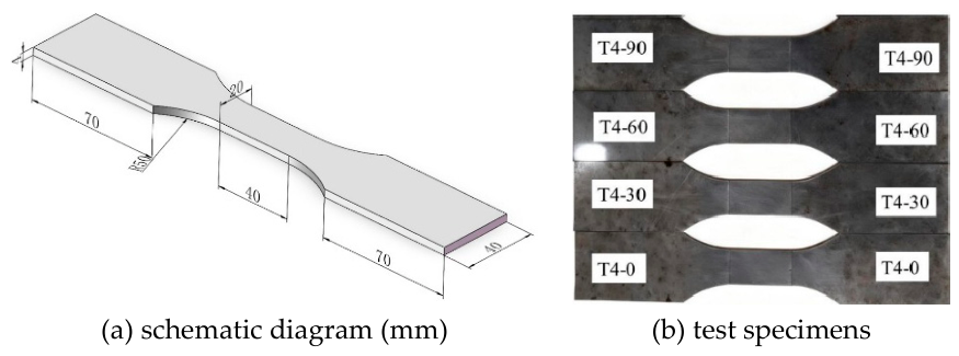
Figure 2.
Accelerated corrosion performance of Q355B steel in different MF strength.
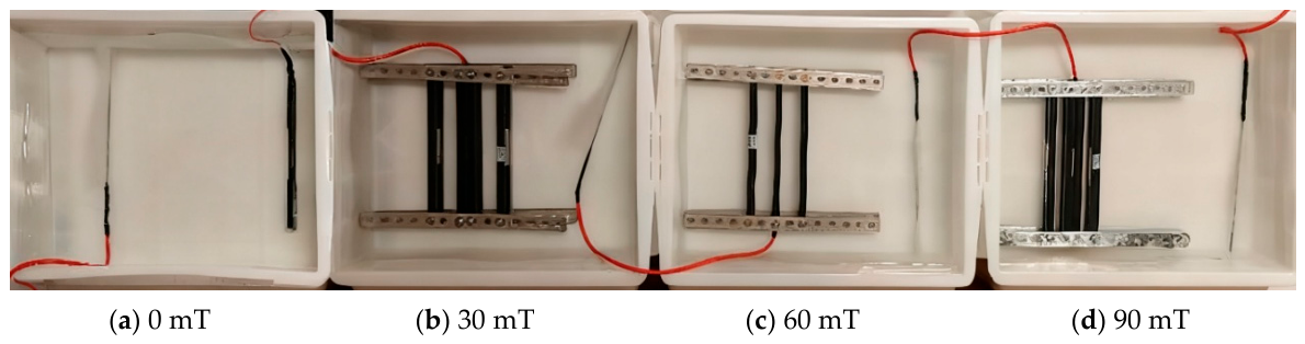
Figure 3.
Macroscopic morphology of the test section of standard specimens after 168 h of accelerated corrosion.
Figure 3.
Macroscopic morphology of the test section of standard specimens after 168 h of accelerated corrosion.
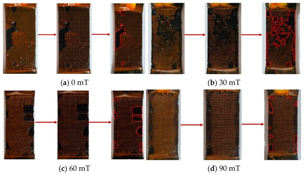
Figure 4.
Variation trends of corrosion mass loss and corrosion rate as a function of magnetic field strength.
Figure 4.
Variation trends of corrosion mass loss and corrosion rate as a function of magnetic field strength.
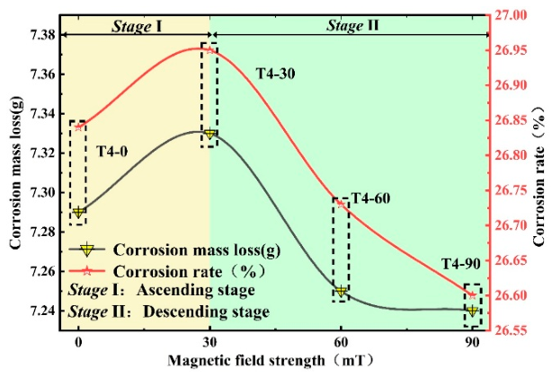
Figure 7.
3D model.
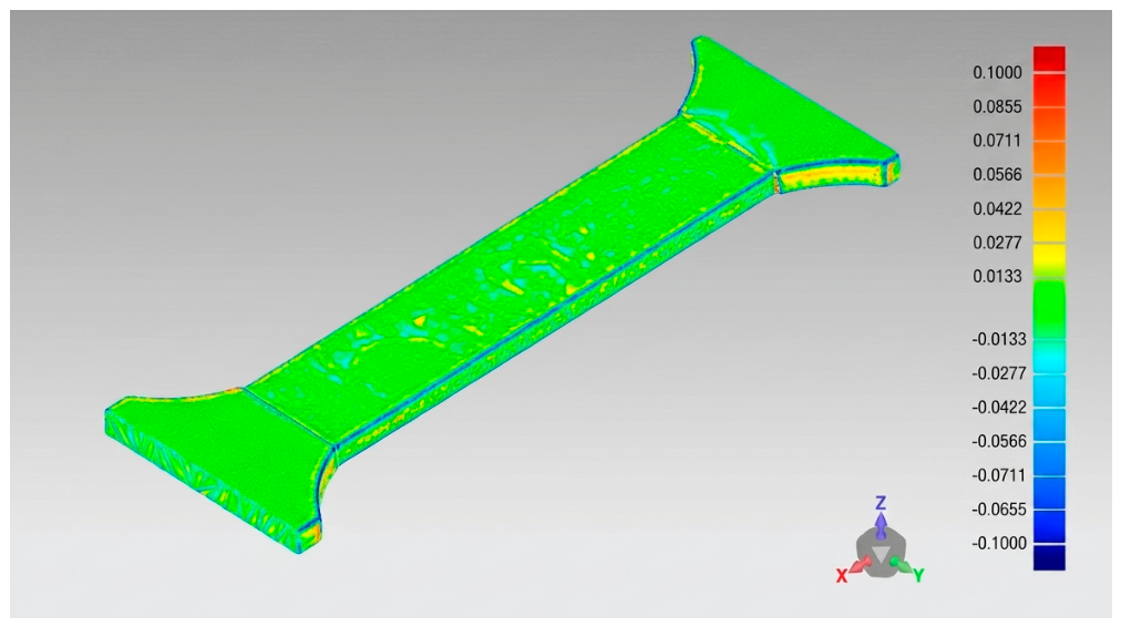
Figure 8.
Point cloud of the test section surface.
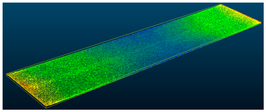
Figure 9.
2D and 3D corrosion morphologies of the 4 mm thick standard specimen test section at various magnetic field strengths.
Figure 9.
2D and 3D corrosion morphologies of the 4 mm thick standard specimen test section at various magnetic field strengths.
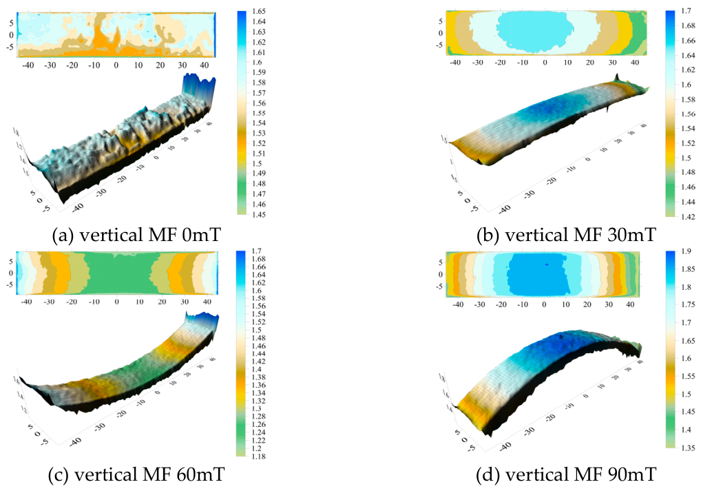
Figure 10.
Normalized autocorrelation functions of corroded surfaces under different magnetic field intensities.
Figure 10.
Normalized autocorrelation functions of corroded surfaces under different magnetic field intensities.
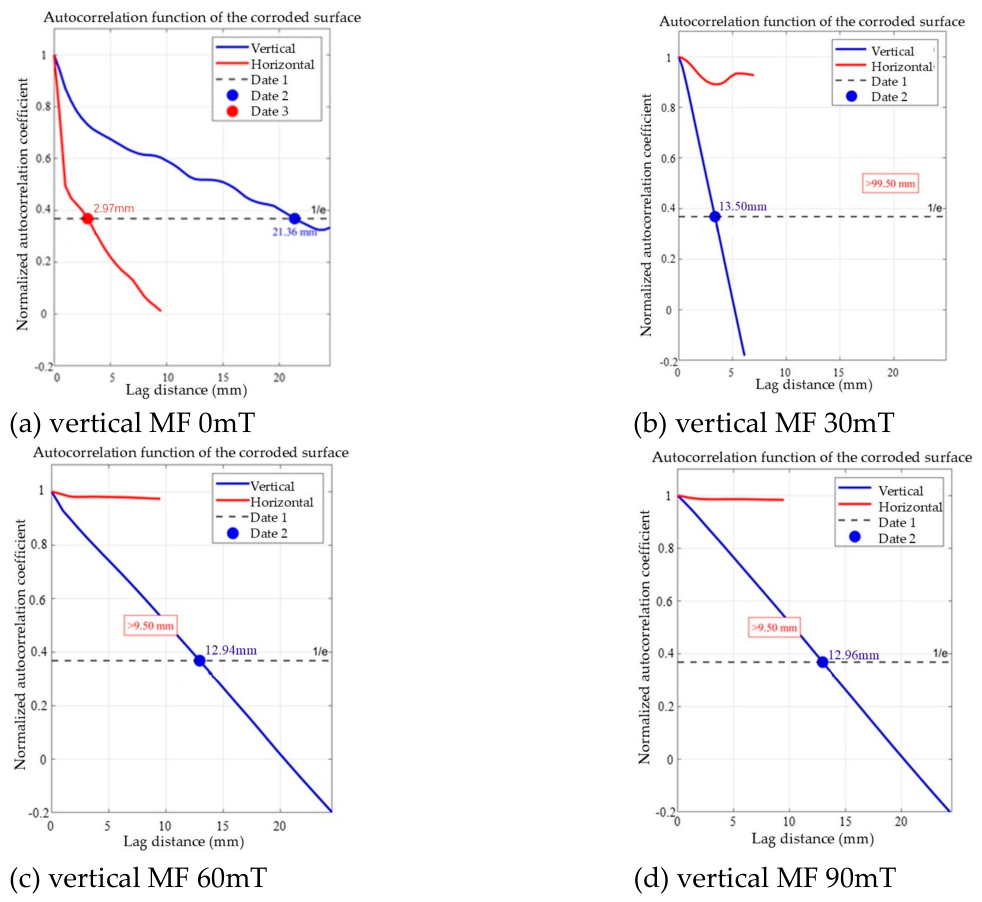
Figure 11.
Probability density distribution fitting of corrosion depth under different magnetic field intensities.
Figure 11.
Probability density distribution fitting of corrosion depth under different magnetic field intensities.
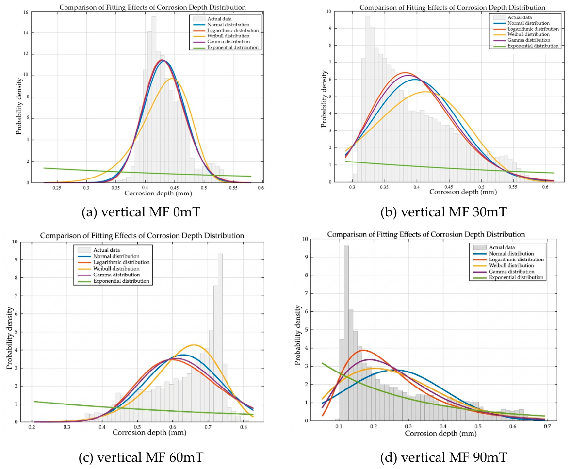
Figure 12.
Geometric model of the helical anchor-soil structure.
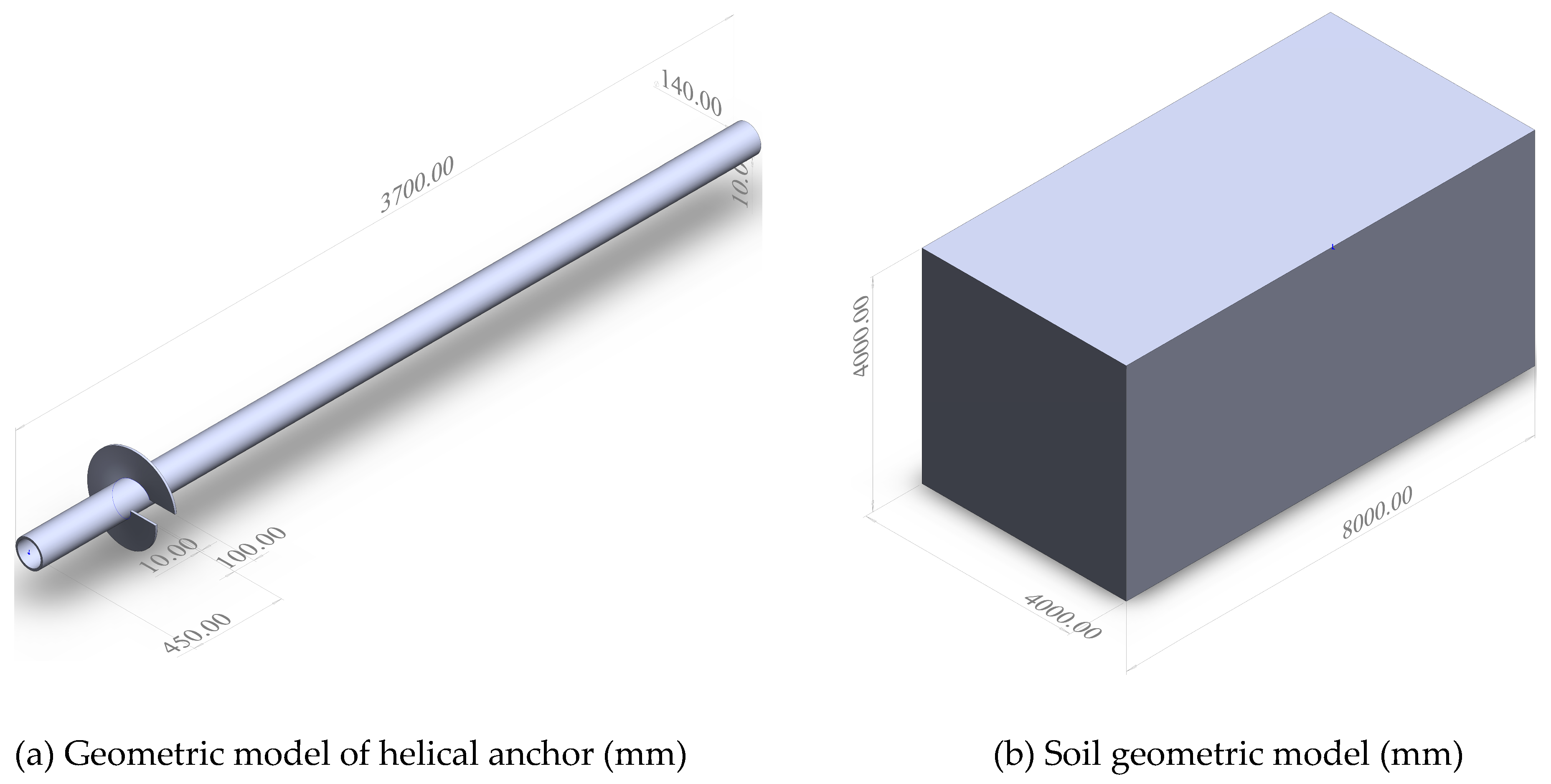
Figure 15.
Comparison of load-displacement curves for helical anchor uplift between numerical simulation and experimental results of literature [51].
Figure 15.
Comparison of load-displacement curves for helical anchor uplift between numerical simulation and experimental results of literature [51].
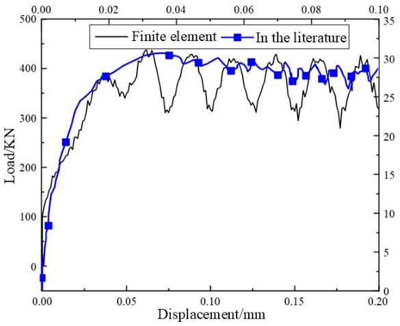
Figure 16.
2D corrosion depth distribution map generated by a random field algorithm.
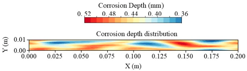
Figure 17.
Comparison of corrosion depth distributions between random field simulation and point cloud-based measurements for helical anchor steel surfaces.
Figure 17.
Comparison of corrosion depth distributions between random field simulation and point cloud-based measurements for helical anchor steel surfaces.
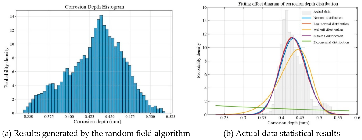
Figure 18.
3D corrosion model of a helical anchor constructed using a Python script-based automated modeling method.
Figure 18.
3D corrosion model of a helical anchor constructed using a Python script-based automated modeling method.
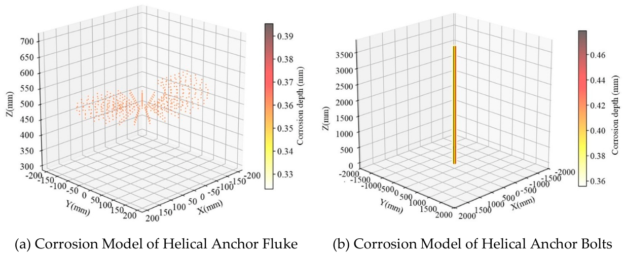
Figure 19.
Uplift load-displacement curves of corroded helical anchors under different magnetic field strengths.
Figure 19.
Uplift load-displacement curves of corroded helical anchors under different magnetic field strengths.
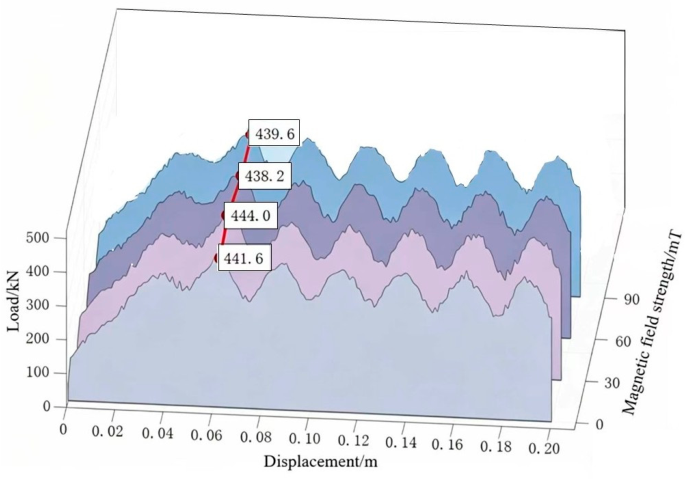
Figure 20.
Equivalent plastic strain (PEEQ) contours of soil surrounding corroded helical anchors under different magnetic field strengths.
Figure 20.
Equivalent plastic strain (PEEQ) contours of soil surrounding corroded helical anchors under different magnetic field strengths.
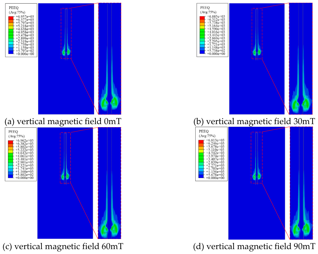
Figure 21.
Vertical compressive stress contours on the upper surface of helical anchor plates under different MF strengths.
Figure 21.
Vertical compressive stress contours on the upper surface of helical anchor plates under different MF strengths.
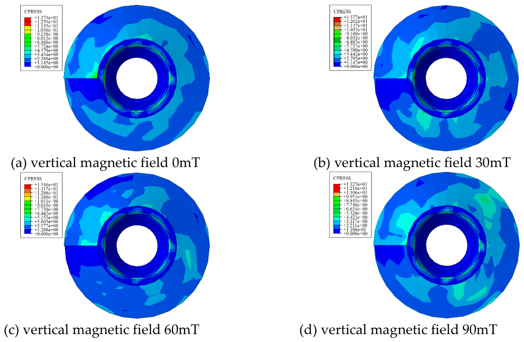
Figure 22.
Contact shear stress distribution on the upper surface of corroded anchor plates under varying magnetic field intensities.
Figure 22.
Contact shear stress distribution on the upper surface of corroded anchor plates under varying magnetic field intensities.
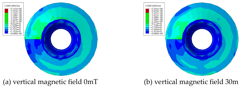
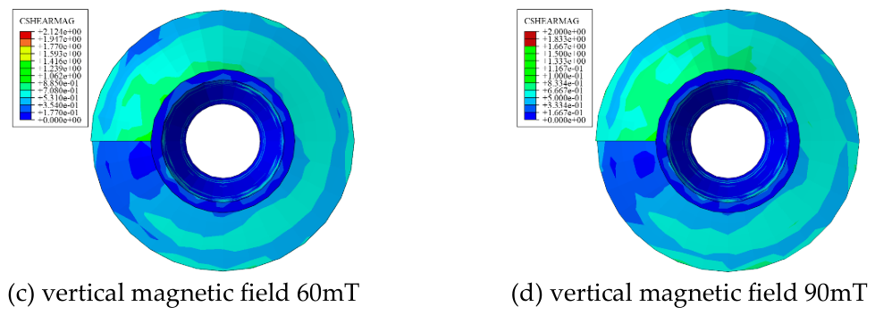

Table 1.
Spatial magnetic flux density calibration across the 40 mm × 20 mm test section.
| Target MF (mT) | Center (mT) | Top-Left (mT) | Top-Right (mT) | Bottom-Left (mT) | Bottom-Right (mT) | Maximum Spatial Deviation (%) |
|---|---|---|---|---|---|---|
| 30 | 30.2 | 29.4 | 29.6 | 29.5 | 29.3 | 2.33% |
| 60 | 60.4 | 58.8 | 59.2 | 58.9 | 58.6 | 2.17% |
| 90 | 90.6 | 87.8 | 88.2 | 88.0 | 87.5 | 2.78% |
Table 2.
Corrosion mass loss rate of the specimens under different MF strengths.
| MF strength | Specimen No. | Initial mass (g) | Mass after corrosion (g) | Test Section Initial Mass (g) | Theoretical mass loss(g) | Individual corrosion rate (%) | Group Corrosion Rate (Mean ± SD) (%) |
|---|---|---|---|---|---|---|---|
| T4-0 | T4-0-1 | 230.21 | 222.94 | 27.14 | 7.27 | 26.79 | 26.84 ± 0.054 |
| T4-0-2 | 230.24 | 222.95 | 27.16 | 7.29 | 26.84 | ||
| T4-0-3 | 230.27 | 222.96 | 27.18 | 7.31 | 26.89 | ||
| T4-30 | T4-30-1 | 230.56 | 223.25 | 27.17 | 7.31 | 26.90 | 26.95 ± 0.044 |
| T4-30-2 | 230.60 | 223.27 | 27.20 | 7.33 | 26.95 | ||
| T4-30-3 | 230.64 | 223.29 | 27.23 | 7.35 | 26.99 | ||
| T4-60 | T4-60-1 | 229.90 | 222.66 | 27.09 | 7.24 | 26.73 | 26.73 ± 0.066 |
| T4-60-2 | 229.93 | 222.68 | 27.12 | 7.25 | 26.73 | ||
| T4-60-3 | 229.96 | 222.70 | 27.15 | 7.26 | 26.74 | ||
| T4-90 | T4-90-1 | 230.72 | 223.49 | 27.19 | 7.23 | 26.59 | 26.60 ± 0.066 |
| T4-90-2 | 230.75 | 223.51 | 27.22 | 7.24 | 26.60 | ||
| T4-90-3 | 230.78 | 223.53 | 27.25 | 7.25 | 26.61 |
Table 3.
Statistics of Geometric Parameters of Corroded Surface Morphology of Specimens.
| specimen | Maximum corrosion depth | Minimum corrosion depth | Average corrosion depth | Standard deviation of corrosion depth | Median corrosion depth | Autocorrelation length in the X direction | Autocorrelation length in the Y direction |
|---|---|---|---|---|---|---|---|
| T4-0 | 0.5805 | 0.2269 | 0.4324 | 0.0350 | 0.4268 | 21.36 | 2.97 |
| T4-30 | 0.6128 | 0.2888 | 0.3971 | 0.0664 | 0.3798 | 13.50 | >9.50 |
| T4-60 | 0.8294 | 0.2072 | 0.6296 | 0.1070 | 0.6621 | 12.94 | >9.50 |
| T4-90 | 0.6928 | 0.0502 | 0.2588 | 0.1428 | 0.2072 | 12.96 | >9.50 |
Table 4.
Recommended Distribution Types and Statistical Parameters.
| Specimen | Recommended distribution type | ||
|---|---|---|---|
| T4-0 | log-normal distribution | -0.841743 | 0.080780 |
| T4-30 | log-normal distribution | -0.936967 | 0.160997 |
| T4-60 | Weibull distribution | 0.672431 | 7.754164 |
| T4-90 | log-normal distribution | -1.493893 | 0.527282 |
Table 5.
Statistical comparison of corrosion depth between random field simulation and point cloud-based measurements.
Table 5.
Statistical comparison of corrosion depth between random field simulation and point cloud-based measurements.
| Statistical Parameter | Measured Results(mm) | Random Field Results(mm) | Simulation Error (%) |
|---|---|---|---|
| Average Corrosion Depth | 0.4324 | 0.4323 | 0.023 |
| Corrosion Depth Standard Deviation | 0.0350 | 0.0343 | 2 |
| Corrosion Depth Median | 0.4268 | 0.4343 | 1.76 |
Disclaimer/Publisher’s Note: The statements, opinions and data contained in all publications are solely those of the individual author(s) and contributor(s) and not of MDPI and/or the editor(s). MDPI and/or the editor(s) disclaim responsibility for any injury to people or property resulting from any ideas, methods, instructions or products referred to in the content. |
© 2026 by the authors. Licensee MDPI, Basel, Switzerland. This article is an open access article distributed under the terms and conditions of the Creative Commons Attribution (CC BY) license (http://creativecommons.org/licenses/by/4.0/).
Copyright: This open access article is published under a Creative Commons CC BY 4.0 license, which permit the free download, distribution, and reuse, provided that the author and preprint are cited in any reuse.


