

Submitted:
02 August 2026
Posted:
03 August 2026
You are already at the latest version
Abstract
A costly process runs to a planned horizon and may be abandoned early by a rule acting on an accruing statistic. Any decision to stop is followed by a fixed operational lag before the stop takes effect. We show that the calendar time recovered by such a rule is a linear functional of its first-passage law against a recoverable-time kernel g(s) = (tend − d − s)⁺, which is convex, non-increasing and identically zero beyond a horizon set by the lag. This yields an exact factorisation of savings into a detection ratio and a timing ratio, and identifies a dead zone in which monitoring is provably worthless. We use it to price the restriction to a single interim look. A single look must trade recoverable time against reliability at a fixed false-stop budget, and cannot do better than the interior optimum of that trade; continuous monitoring is not so constrained. We also show that the reliability-optimal futility boundary is the one-sided sequential probability ratio boundary of Wald, recovered here from a time-recovery objective rather than an error-rate one. In a worked example calibrated to non-oncology phase III trials, continuous monitoring averts 55% of a doomed trial's duration against 43% for the best single look at matched budget (a factor of 1.28) and 37% for the deployed conditional-power convention at the conventional midpoint (a factor of 1.50). Computing the probability of stopping a trial that would in fact have succeeded as a joint rather than a product measure — the two events are strongly negatively dependent — we find continuous monitoring also incurs less such regret than either single look at every effect size examined, so the comparison is not a trade but a dominance on both axes. The advantage is stable in the lag, and we are explicit about which claims are structural and which are numerical.
Keywords:
optimal stopping
; first passage
; sequential analysis
; futility
; interim monitoring
; group-sequential design
; stochastic curtailment
1. Introduction
1.1. The Problem
Consider a process committed to in advance, running at continuous cost, which can be recognised part-way through as unlikely to achieve its purpose. The commitment fixes a horizon; the cost accrues whether or not the purpose remains attainable; the recognition, if it comes, arrives gradually and noisily. Two questions follow: when should one look, and what is forgone by looking only once?
The setting is generic. Its clinical instance—a randomised trial whose treatment arm is heading to futility while continuing to enrol patients who cannot benefit—motivates the case study of Section 8, but is a special case rather than the subject. A policy programme with a fixed review cycle, a campaign with a booked media buy, a military commitment with a declared objective, and a failing marriage share the structure: a planned end, an accruing but noisy indication of the eventual outcome, a period before that indication can be trusted, and a lag — often bureaucratic, sometimes merely human—between deciding to stop and stopping. What differs is the currency in which recovered time is denominated. We work in the currency-free unit of calendar time and convert once, in the case study.
1.2. Schemes and Notation
The process runs from to , with , and is in one of two unobservable states: , doomed, meaning it would not have achieved its objective, or , meaning it would. We compare three schemes: no interim assessment; a single fixed look at a prespecified information fraction ; and continuous monitoring. Every trigger, under every scheme, is followed by the same fixed lag d before the stop takes effect. In the clinical instance : convene the committee, unblind and verify, then implement.
We write for information fraction, which under constant recruitment with a continuous endpoint is linear in calendar time.
1.3. Contributions
The recoverable-time kernel of Section 2, with its dead zone and last-useful-trigger horizon, appears to be new, as does the resulting exact factorisation of savings into detection and timing (Proposition 1), which we propose as a reporting device for monitoring committees. The joint-measure treatment of false-stop regret in Section 7 corrects an approximation that is easy to make and materially misleading.
Three things are not new and we mark them plainly. That binding futility boundaries cannot inflate type-I error is standard [8]. The optimal boundary we derive in Section 6 is the one-sided sequential probability ratio boundary of Wald [18]; our contribution there is only that it arises from a time-recovery objective under lag rather than from an error-rate criterion, and Whitehead’s triangular test [20] and Anderson’s modified SPRT [1] are close relatives. Nor is monitoring under delayed information unexamined: Hampson and Jennison [7] treat group sequential tests for delayed responses, and there is an established literature on overrunning. What we add is the observation that the lag induces a horizon past which monitoring recovers nothing, and that this horizon is the right object against which to price the frequency of looks.
1.4. Related Work
Sequential analysis begins with Wald’s probability ratio test [18] and its optimality [19], and continues through Chernoff [3], Anderson [1], Siegmund [17] and Shiryaev [16]. Group-sequential designs for clinical trials—O’Brien and Fleming [13], Pocock [14], the -spending generalisation of Lan and DeMets [9]—address multiplicity created by efficacy looks at a small number of prespecified times. Stochastic curtailment and conditional power [10,15] supply the standard futility machinery; Whitehead [20] and Jennison and Turnbull [8] give the canonical syntheses. The first-passage apparatus is due to Bachelier [2] and Lévy [12] for linear boundaries, with the general characterisation from Fortet [6] and Durbin [5].
2. The Recoverable-Time Kernel
2.1. The Delay Operator
A trigger at time s does not stop the process at s: it initiates a review-and-implementation sequence of fixed duration d, so the process halts at , the minimum reflecting that a stop cannot be executed after the process would have ended anyway. The time recovered is
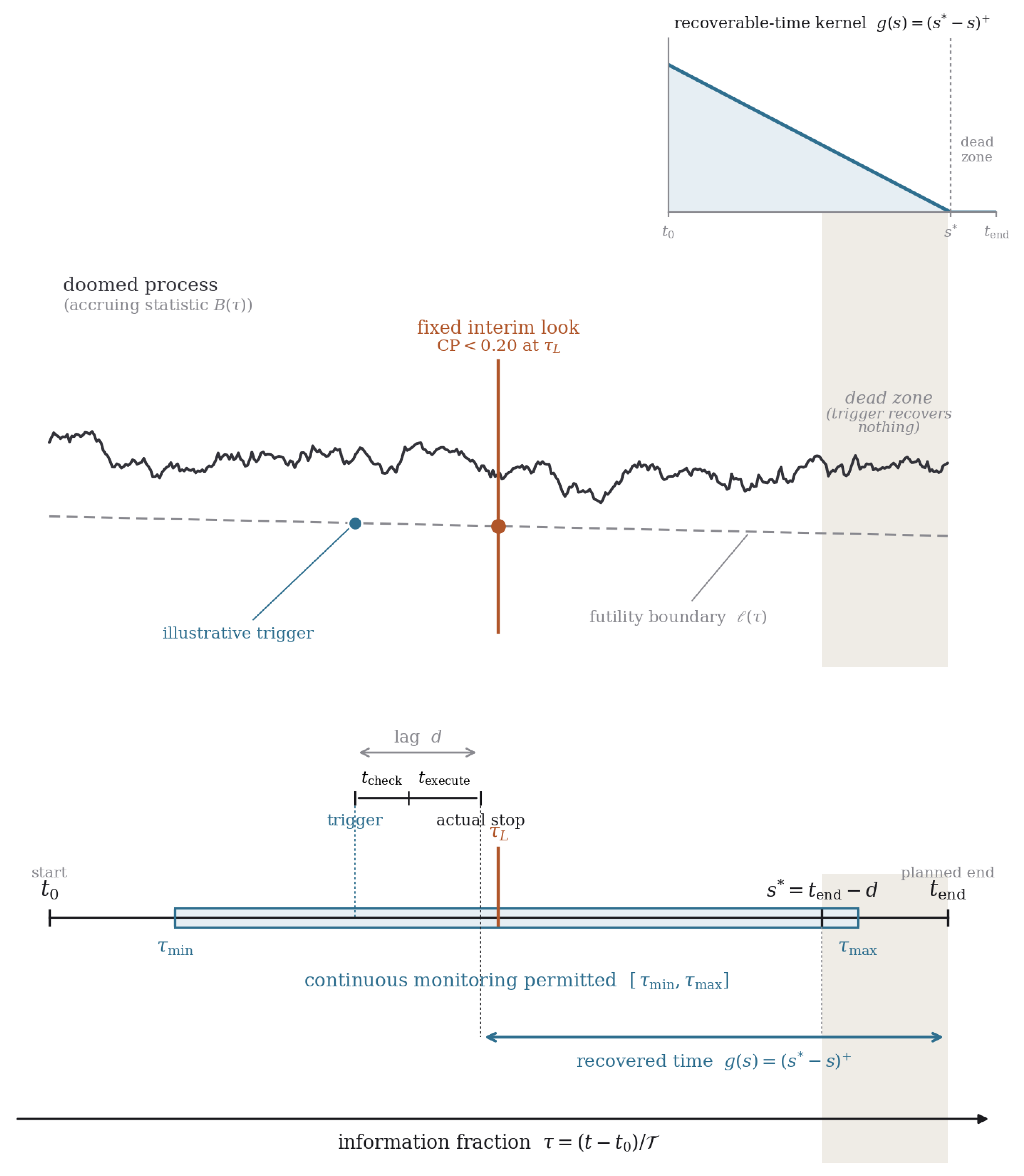
the recoverable-time kernel: non-increasing, convex, linear with slope on , and identically zero on . All delay physics live in the single kink at , the last useful trigger time (Figure 1). In dimensionless form with , , .
2.2. Savings as a Linear Functional
A scheme in state is described by a sub-probability trigger law on with mass ; Section 4 constructs it as a first-passage density, but nothing here depends on how it arises. Since a trigger at s recovers and no trigger recovers nothing,
with S distributed as . A single look at is the degenerate case , giving .
Two consequences. First, error rates live entirely in the mass and monitoring geometry entirely in the kernel average, so no part of the time saved is entangled with the error accounting; a scheme cannot appear to save time by quietly relaxing its error rates. Second, because g vanishes beyond , trigger mass there contributes exactly nothing: the effective monitoring ceiling is , and extending a window past is waste. The lag sets the horizon past which monitoring is pointless.
We report the two states separately throughout. is time saved by correctly abandoning a doomed process; is time “saved” by stopping one that would have succeeded, which is a cost. Section 7 shows the latter is properly measured as a joint probability, not as the mass .
3. Comparing Schemes
3.1. The Exact Decomposition
Fix and suppose and , so . Define the detection ratio and timing ratio
Proposition 1
(Detection–timing factorisation). , so continuous monitoring saves more time than the single look precisely when .
Proof.
Immediate from (1): . □
This is a definition rearranged, not a theorem, and we claim nothing more for it than that. Its value is as a reporting device: it separates a comparison that is usually made as a single opaque number into one factor an error-rate audit can check () and one a scheduling argument can check (), each interpretable alone. Section 8 reports both.
One structural remark is worth recording, because it explains why dispersion in trigger time is not penalised. Writing pointwise and taking expectations gives, whenever ,
the second term being non-negative and strictly positive exactly when the trigger law places mass beyond . Because a late trigger is worthless rather than harmful—g is floored at zero, never negative—spreading mass across the kink can only raise the average. A rule whose mean trigger time is slightly later than a single look’s may still recover more.
3.2. What a Single Look Cannot Escape
It is tempting to argue that continuous monitoring reaches a region of recoverable time structurally closed to any single look, by comparing an oracle continuous rule firing at against an oracle look at and reading off . That argument is circular, and we do not make it: is a design variable, and setting reduces the gap to zero. It shows only that a later look recovers less than an earlier one, which has nothing to do with continuity.
The real constraint on a single look is a trade it cannot avoid, and it appears only once the false-stop budget is held fixed. Let the budget be , so a look at must use the threshold with . Then the detection probability is
for a doomed state at the null and a design alternative , which is increasing in : looking later is more reliable. But is decreasing: looking later recovers less. The single look must therefore maximise the product
which has an interior maximum. Continuous monitoring faces no such scalar choice: it distributes trigger mass across the window and its benefit is the full integral .
Whether the integral beats the best point is a quantitative question, not a theorem, and it depends on , and . We answer it numerically in Section 8, where the optimum of (3) sits at and continuous monitoring exceeds it by a factor of . We regard this as the honest form of the comparison and report it as the headline, alongside the larger factor of against the conventional midpoint look, which is a claim about practice rather than about single looks in principle.
4. The Stopping Law
4.1. The Monitored Process
Under constant recruitment with a continuous endpoint, information accrues linearly in calendar time, so is the natural clock. We monitor the B-value process [11]
with the expected final z-score: for a process that would succeed, for a doomed one. Futility is a lower boundary ; the rule triggers at the first monitored with . Write for the drift gap and for the mean drift.
4.2. First Passage as the Primitive
Let and let be its sub-density, . Three objects must be distinguished: the marginal , the cumulative first passage , and the cumulative hazard . They are ordered.
Lemma 1
(Sandwich). for all τ.
Proof.
gives the left inequality. For the right, by on . □
The lemma locates two errors that are easy to make. Treating the marginal as the cumulative stopping probability understates risk; summing marginal rates as though looks were independent overstates it, the gap being the re-counting of one sustained excursion at many correlated looks. Neither proxy is used below.
4.3. General Boundaries, and the Exact Linear Case
Conditioning on the first touch gives Fortet’s equation [6], an exact Volterra equation of the first kind:
with p the transition density. Letting and differentiating gives Durbin’s representation [5], : the first-passage density tracks the boundary density, not the tail. Durbin’s representation is exact; the Daniels tangent approximation is not, in general.
For a linear boundary it is. Take with and set , Brownian with drift started at . First passage to zero has the Bachelier–Lévy density
and since , dividing by gives
independent of drift, hence common to both states. The tangent value is exact for a straight boundary because the tangent is the boundary; this, rather than convenience, is why we use the linear case for closed forms. (Note the sign: for a lower boundary with the rate is , as a first-passage rate must be.)
The crossing probabilities read the two ledgers directly: over an infinite horizon when (doomed, drifting into the boundary) and when (a would-be winner drifting away). Windowed to the exact values come from the inverse-Gaussian distribution function (Appendix B); the difference matters, and we use windowed values throughout the case study rather than the infinite-horizon approximation.
4.4. Which Ledger Takes the Kernel
Benefit is time-discounted: a doomed process abandoned at s saves . Cost is not: a process wrongly stopped is stopped, and the loss does not depend on when. So the kernel weights the ledger only,
and the cost is a joint probability over the path, not the mass . Section 7 computes it.
5. Type-I Error
Declare success at if , and let , so the unmonitored type-I error is . Let be the set of instants at which futility is checked, and under a binding rule
Theorem 1
(Non-inflation; monotone in the monitoring set at fixed boundary). For a fixed boundary ℓ and monitoring sets ,
Proof.
Enlarging adds survival constraints, so ; probabilities order accordingly. □
This is standard [8] and we claim it only as a premise. Two qualifications matter, and both cut against the natural extension of the result.
First, Theorem 1 compares monitoring sets at a fixed boundary. It does not order two schemes with different boundaries, and the ordering can go either way. In the worked example of Section 8, at the single conditional-power look deflates type-I error by while the continuous rule deflates it by : the single look deflates more, because it is a more aggressive cut at the one time it acts. Any claim that continuous monitoring protects better than a single look is unsupported in general and false here. What survives, and is all we use, is that neither inflates.
Second, the freed mass can be banked as conservatism or recovered as power, but not both, and the two options are not equally safe. Under non-binding accounting—computing as though the boundary were absent—a futility stop can only remove a rejection that would otherwise have counted, so realised type-I error is at most nominal whether or not the committee honours the stop. That override-robustness holds at unchanged . If instead the efficacy threshold is lowered to recover power (here to ), a single honoured override admits realised up to , some above nominal. The two guarantees are incompatible, which is why regulators do not permit recovery from futility boundaries. We therefore bank the deflation and take no credit for it anywhere in the case study.
For scale, the deflation is small: for the continuous design of Section 8, against one-sided. Its magnitude depends on boundary aggressiveness; only its sign is guaranteed.
6. The Optimal Boundary Is the SPRT Boundary
6.1. Purity and the Likelihood Ratio
A rule that fires on first passage should be judged not by how often it fires but by what a firing implies. Define stop-purity
with . For the linear boundary the Durbin rate is drift-free and cancels, leaving the Gaussian exponents. The result is immediate from Girsanov: the likelihood ratio of the path is , and evaluating it on gives
Two consequences follow, and neither is deep, but both are useful. The intercept means a crossing is self-certifying: crossing a boundary at depth is evidence of low drift however early it occurs, which is information a fixed look—seeing only the level , not the event of having crossed—discards. And purity increases in only if : a futility boundary climbing faster than the mean drift begins catching winners late, so late stops lose diagnosticity.
6.2. The Design Problem
The trigger law is not chosen; it is the first passage across a boundary. The design variables are therefore the boundary geometry and the window. For a winner the crossing probability is , falling exponentially in depth; for a doomed process passage is near-certain and depth is paid in time, . Benefit therefore falls linearly in while cost falls exponentially, so a false-stop budget binds, giving and expected detection time . Maximising the denominator over m:
Proposition 2
(Optimal boundary). Expected detection time is minimised at
Remark 1
(This is Wald’s boundary). By (5), is exactly the condition that be constant in τ: the level sets of the path likelihood ratio in B-space are straight lines of slope , so the optimal futility boundary is a level set of the likelihood ratio—the one-sided boundary of Wald’s sequential probability ratio test [18,19]. That stop-purity is then constant across the window is the defining property of a likelihood-ratio boundary, not an emergent coincidence. We claim no novelty for the boundary. What is perhaps of interest is the route: the SPRT boundary is recovered here by minimisingtime to detection under a false-stop budget, an objective in the currency of recoverable calendar time, rather than by the error-rate criterion under which it is usually derived. Whitehead’s triangular test [20] and Anderson’s modified SPRT [1] are the closest relatives in the clinical-trials literature, both employing straight-line boundaries on essentially this scale.
Two caveats on Proposition 2, since the paper’s numbers depend on them. It minimises , a proxy, rather than the stated objective ; and the depth formula uses the infinite-horizon crossing probability. Both are close but neither is exact. For the case-study parameters the closed form gives whereas solving the windowed budget numerically gives , and numerically optimising the true objective over gives with a benefit only above the proxy design. We use the numerically solved values throughout Section 8 and quote Proposition 2 as the structural statement it is: depth logarithmic in the budget, detection time inverse-quadratic in the drift gap.
Finally, at the purity (5) is constant, so the admissibility condition is a -free inequality: it holds everywhere or nowhere, and no reliability floor is induced. This is a genuine simplification but also a limitation—the purity apparatus is inoperative at the recommended design, and becomes a matter of external constraint (minimum enrolment, data quality) rather than of inference. Section 8 states the achieved purity explicitly.
7. Mixtures and the Measurement of Regret
7.1. The Binary State Is a Projection
Let mean that the process, run to , would not have declared success—a functional of the completed path, not a latent parameter. A doomed-looking process that recovers is then a realisation whose statistic dipped below the boundary on its way to success, and is counted in the cost ledger by construction.
Let the true drift carry a prior G. Since (1) is linear in the trigger law and the trigger law of a mixture is the mixture of trigger laws, every result above integrates through: . The two-point model is a projection, not an assumption. What the mixture demands is a richer reporting standard than a single detection rate: the futility power curve , tabulated in Section 8.
7.2. Regret Is a Joint Probability, Not a Product
The quantity of interest is the probability of stopping a process that would have succeeded,
It is tempting to factor this as . That is wrong, and badly so: the two events are strongly negatively dependent, since a path that dips to a deep futility boundary is much less likely to finish high. For a linear boundary the joint probability is available exactly.
Proposition 3
(Exact regret for a linear boundary). For and boundary ,
Proof.
Let , Brownian with drift from ; a trigger is first passage of Z to zero. Since , the event is with . By Girsanov and the reflection principle, for and the density of on is , whence . Substituting gives the result. □
The correction is large. At the case-study parameters the product form overstates regret by factors of , and at , and respectively, and it displaces the peak of the regret curve from to (Section 8). Monte Carlo agrees with Proposition 3 to simulation error.
Remark 2
(Where regret falls). Regret does not concentrate on negligible treatments. The two factors run oppositely — decays in ϑ, the probability of eventual success rises—so the product peaks in the interior, and at the case-study parameters it peaks near , about of the design effect. Below that, candidates are stopped often but would mostly have failed anyway; above it, they would have succeeded but are rarely caught. Any claim that futility monitoring discards only worthless candidates is unsupportable, and the burden falls on every futility rule, the deployed convention included. What is true is narrower: regret is self-limiting at the upper end, falling to under a fifth of its peak beyond , so a clearly effective therapy is seldom abandoned. The exposure is to moderate effects, which is the regime a confirmatory trial exists to adjudicate.
8. Case Study: A Non-Oncology Phase III Trial
8.1. Setting
We take a non-oncology phase III trial with a continuous endpoint measured at fixed follow-up and constant recruitment, so that information accrues linearly in calendar time as the framework assumes. Trials with time-to-event endpoints are excluded, since there information accrues with the event count rather than the clock and the kernel would no longer be linear in ; that case is an extension rather than an instance (Section 10).
8.2. The Comparator
The deployed futility convention is to stop if conditional power falls below at a single prespecified interim [10,15]. Under the current-trend (maximum likelihood) projection—we state the choice explicitly, as protocols also use design-alternative and null projections, which shift the threshold —
so the rule is a lower-boundary crossing and enters the framework with no new apparatus.
We report two comparators, because they answer different questions. The deployed convention is at the conventional midpoint . The best single look is the maximiser of (3) over at the same false-stop budget, which is the honest methodological benchmark. Conflating them inflates the apparent advantage, and we keep them separate throughout.
8.3. Parameters
The provenance of d is weak: convening-to-decision latency is not systematically reported, and two months is a judgement. Section 8.7 varies it from a fortnight to six months. The per-patient cost enters only the currency conversion in Section 8.9 and no structural claim depends on it. The base rate does not enter the headline comparison at all.
| symbol | value | basis |
| 36 months | phase III typically 1–4 years | |
| N | 500 patients | phase III commonly 300–500 |
| cost/patient | $60,000 | published per-patient phase III costs, ≈$40k–113k [4] |
| 3.24 | power, two-sided : | |
| 0 | doomed = exact null (the least favourable case) | |
| conditional-power convention | ||
| d | 2 months | committee convening, interim lock, implementation; |
| 0.40 | phase III attrition [21]; enters purity and portfolio figures only |
8.4. Operating Characteristics
At the conditional-power boundary sits at , giving a marginal stopping probability at the design alternative of and detection at the null of . We adopt as the common false-stop budget: it is the tolerance that current practice reveals itself to accept. The continuous arm is then solved numerically for at , giving windowed masses and .
8.5. Results
Against the best single look the factor is ; against the deployed convention it is . The gap between those two numbers is itself a finding: the conventional midpoint interim is badly placed. Simply moving the single look from to , at unchanged false-stop risk, recovers of the months that separate the convention from continuous monitoring—with no continuous monitoring whatsoever. We regard as the methodological claim and as the claim about current practice, and neither should be quoted without the other.
| scheme | detection | averted exposure | months | patients | |
| no interim | — | — | 0 | 0 | 0 |
| , deployed convention | 185 | ||||
| best single look, matched budget | 217 | ||||
| continuous, matched budget | — |
Proposition 1 decomposes the advantage over the best single look: and , product . Continuous monitoring wins on detection and gives back a little on timing, since the best single look is deliberately placed early. Against the deployed convention the decomposition is , : there it wins mostly on timing.
8.6. Regret, Measured Jointly
Using Proposition 3 and the corresponding bivariate-normal calculation for a single look, the probability of stopping a trial that would have succeeded is:
| continuous | at | best look at | |
Continuous monitoring incurs less regret than either single look at every effect size up to the design alternative, despite being matched to them on marginal stopping probability at . The reason is that matching marginals does not match joints: a look at acts on one-third of the information and catches paths that would have recovered, whereas the continuous rule acts on the running minimum and catches paths that genuinely trend down. At the design alternative the continuous rule stops roughly one in 22 trials that would have succeeded, against one in 21 for the deployed convention and one in 17 for the best single look.
The comparison is therefore not a trade. On this pair of axes—exposure averted and would-be winners stopped—continuous monitoring dominates both single-look designs simultaneously, and no adjustment of the boundary depth is required to purchase the second axis.
8.7. Sensitivity to the Operational Lag
Both arms re-solved at matched budget for each lag:
| d (months) | convention | best look () | continuous | vs. best | vs. convention | |
| () | ||||||
| 1 | () | |||||
| 2 | () | |||||
| 3 | () | |||||
| 4 | () | |||||
| 6 | () |
The advantage over the best single look is essentially invariant in the lag, at – throughout; the advantage over the deployed convention grows with it, because a fixed midpoint look sits further into the dead zone as d rises while the optimal look time drifts earlier. A slow committee is not an argument against continuous monitoring, but neither does it much amplify the methodological case.
8.8. Purity of the Recommended Design
At the constant stop-purity of Section 6 is , giving
We state this plainly because it constrains the design. At the achieved purity is : of every hundred stops, roughly thirteen are of processes that would have succeeded. A committee demanding at must tighten the budget to , which deepens the boundary to and reduces averted exposure to —against for the best single look at that budget, a factor of . The comparison is unchanged; only the absolute figures move.
Note that this purity is inherited from the deployed convention, whose budget we adopted. The conditional-power rule at operates at the same and therefore at comparable purity. If is judged inadequate, the finding indicts current practice at least as much as the proposal.
8.9. Impact
Converting at and $60,000 per patient, and comparing against the best single look: months, 60 patients and $3.6M per doomed trial. Against the deployed convention: months, 92 patients and $5.5M. At a portfolio failure rate of the corresponding shares of total phase III calendar time reclaimed are for continuous monitoring, for the best single look and for the convention.
8.10. What the Example Establishes
Under sourced non-oncology phase III parameters, with both comparators held to the false-stop budget that current practice reveals it accepts, with the doomed state at the least favourable exact null, and taking no credit for the type-I deflation of Section 5: continuous monitoring averts about half of a doomed trial’s duration, exceeding the best single look by and the deployed convention by , while stopping fewer would-be winners than either. The first factor is stable in the lag; the second grows with it.
It does not establish that the advantage is large under all parameters. It narrows as the doomed state approaches the design alternative, and the currency conversion depends on cost inputs we have not independently verified. The structural claims—the dead zone, the factorisation, the joint measurement of regret—do not depend on any of these.
9. Discussion
9.1. What the Analysis Supports
Three claims are structural and do not depend on the case-study parameters. The operational lag induces a horizon beyond which monitoring recovers nothing, so a monitoring window extending past it is waste and the lag is the natural unit in which to price the frequency of looks. Savings factor exactly into a detection ratio and a timing ratio, which we recommend reporting separately. And the probability of stopping a process that would have succeeded is a joint probability over the path; factoring it as a product of marginals overstates it by factors of two to five in the regime that matters, and displaces the peak of the regret curve by about a fifth of the design effect.
Two claims are numerical, and we have tried to state them at the strength the arithmetic supports and no higher. Continuous monitoring exceeds the best single look at matched budget by about of averted exposure, stably in the lag; it exceeds the deployed conditional-power convention at the conventional midpoint by about , increasingly in the lag. Roughly a third of the second figure is available simply by moving the conventional interim earlier.
One claim we withdraw. An earlier form of this argument compared oracle ceilings and concluded that a region of recoverable time was structurally closed to any single look. That comparison is circular, since the look time is a design variable; setting it equal to the earliest admissible monitoring time closes the gap exactly. Continuity does not enter. What remains is the interior trade of (3), which a single look genuinely cannot escape but which bounds its loss at a quantity we can only compute, not bound in closed form.
9.2. Beyond Clinical Trials
The kernel is a statement about the value of recovering time net of a wind-down lag, and applies wherever a committed process can be abandoned: a policy programme whose review cycle plays the role of ; a campaign whose contracted media buy sets and whose cancellation notice sets ; a military commitment whose withdrawal timetable is the lag.
The case of a failing marriage is worth stating explicitly rather than as a flourish, because it isolates the parameters unusually clearly. The base rate is high; the accruing statistic is noisy and its early values untrustworthy, so a reliability floor is genuine rather than conventional; the lag between deciding and separating is substantial and largely administrative; and the asymmetry of Section 4 is stark, in that the cost of a wrong stop is not discounted by how late it occurs. The framework says that a single scheduled review—the annual reckoning, the counselling appointment at a fixed date—must solve the same interior trade as any other single look, and that its loss relative to continuous attention does not shrink because the separation process is slow.
9.3. Limitations
The lag is a known constant; in practice it is random and plausibly correlated with trigger time. The confirmatory review is modelled as a single gate with no error of its own. The closed forms assume a Brownian statistic with linear information accrual and a linear boundary. Efficacy stopping, multi-arm designs and sample-size re-estimation are out of scope. The comparison of averted exposure treats calendar time as the objective; a full decision analysis would weight patient-years against the option value of a treatment not abandoned, which we have not attempted.
9.4. Extensions
Event-driven processes, where information accrues with events rather than calendar time, would extend the framework to time-to-event endpoints, replacing the linear clock with an event clock and rebuilding the kernel; this is the most valuable next step and would connect to the delayed-response literature [7]. A random lag would smooth the kink at and, by (2), plausibly increase rather than decrease the value of dispersed trigger mass. Permitting more than one confirmatory look would interpolate between the architecture studied here and full group-sequential monitoring.
10. Conclusions
The operational lag between deciding to stop a process and stopping it induces a horizon beyond which monitoring recovers nothing, and the time a stopping rule recovers is a linear functional of its first-passage law against the kernel . This yields an exact factorisation of savings into detection and timing, and it prices the restriction to a single interim look: such a look must solve an interior trade between recoverable time and reliability at a fixed false-stop budget, which continuous monitoring is not obliged to solve. The reliability-optimal futility boundary turns out to be Wald’s one-sided sequential probability ratio boundary, recovered here from a time-recovery objective. In a non-oncology phase III example, continuous monitoring averts of a doomed trial’s duration against for the best single look at matched budget and for the deployed conditional-power convention, while stopping fewer trials that would in fact have succeeded—a difference visible only when that regret is measured as a joint probability over the path rather than as a product of marginals.
The most useful extension is to trials whose information accrues with events rather than with the calendar: time-to-event endpoints, and oncology trials in particular, require the kernel to be rebuilt on an event clock and would connect this analysis to the delayed-response literature [7]. Single-arm and multi-arm designs are also natural targets, the latter raising the question of how recoverable time should be allocated when one arm of several is abandoned. A random rather than fixed lag, and more than one confirmatory look, are the two obvious refinements within the present setting.
Appendix A. Comparison Identities
Proposition 1. From (1), .
Equation (2). For every real x, , so pointwise . Taking expectations, , and when the first term equals . The remainder is non-negative, and strictly positive iff the trigger law places mass beyond .
Appendix B. First Passage for a Linear Boundary
Durbin’s rate. With , is Brownian with drift from , and first passage to zero has density (4). Since and , the ratio is , independent of .
Windowed masses. The inverse-Gaussian distribution function with , is
and . The benefit functional is with the zeroth and first partial moments of on . All case-study values are computed from these windowed expressions, not from the infinite-horizon approximation , which differs by about at the relevant parameters.
Appendix C. Type-I Error
Theorem 1. Enlarging the monitoring set adds survival constraints, so and probabilities order accordingly; . Strictness holds whenever the set of paths that cross ℓ on yet finish above has positive Wiener measure.
Non-binding accounting. Computing as though the boundary were absent compares at the same efficacy threshold, so a futility stop can only remove a rejection; realised type-I error is at most nominal irrespective of override. This holds at unchanged only.
Magnitude. By Proposition 3 at , the deflation for the continuous design of Section 8 is ; the corresponding bivariate-normal calculation for the conditional-power look at gives .
Appendix D. Purity and the Likelihood Ratio
By Girsanov the path likelihood ratio for drift against is . Evaluated on this gives (5). Equivalently, the Durbin prefactor is drift-free and cancels in , leaving the difference of Gaussian exponents, , which reduces to the same expression using and . Admissibility is ; at this is free of .
Appendix E. The Design Problem
With and , benefit falls linearly and cost exponentially in , so the budget binds at and detection time is . The denominator is concave in m with derivative , vanishing at with value , giving Proposition 2. Numerically optimising the exact objective over subject to the windowed budget gives against the proxy’s , with benefit higher by .
References
- Anderson, T.W. (1960). A modification of the sequential probability ratio test to reduce sample size. Annals of Mathematical Statistics, 31(1), 165–197. [CrossRef]
- Bachelier, L. (1900). Théorie de la spéculation. Annales Scientifiques de l’École Normale Supérieure, 17, 21–86. [CrossRef]
- Chernoff, H. (1961). Sequential tests for the mean of a normal distribution. Proc. Fourth Berkeley Symposium, 1, 79–91.
- DiMasi, J.A., Grabowski, H.G. and Hansen, R.W. (2016). Innovation in the pharmaceutical industry: new estimates of R&D costs. Journal of Health Economics, 47, 20–33. [CrossRef]
- Durbin, J. (1985). The first-passage density of a continuous Gaussian process to a general boundary. Journal of Applied Probability, 22(1), 99–122. [CrossRef]
- Fortet, R. (1943). Les fonctions aléatoires du type de Markoff associées à certaines équations linéaires aux dérivées partielles du type parabolique. Journal de Mathématiques Pures et Appliquées, 22, 177–243.
- Hampson, L.V. and Jennison, C. (2013). Group sequential tests for delayed responses. Journal of the Royal Statistical Society B, 75(1), 3–54.
- Jennison, C. and Turnbull, B.W. (2000). Group Sequential Methods with Applications to Clinical Trials. Chapman and Hall/CRC.
- Lan, K.K.G. and DeMets, D.L. (1983). Discrete sequential boundaries for clinical trials. Biometrika, 70(3), 659–663. [CrossRef]
- Lan, K.K.G., Simon, R. and Halperin, M. (1982). Stochastically curtailed tests in long-term clinical trials. Sequential Analysis, 1(3), 207–219. [CrossRef]
- Lan, K.K.G. and Wittes, J. (1988). The B-value: a tool for monitoring data. Biometrics, 44(2), 579–585. [CrossRef]
- Lévy, P. (1948). Processus Stochastiques et Mouvement Brownien. Gauthier-Villars, Paris.
- O’Brien, P.C. and Fleming, T.R. (1979). A multiple testing procedure for clinical trials. Biometrics, 35(3), 549–556. [CrossRef]
- Pocock, S.J. (1977). Group sequential methods in the design and analysis of clinical trials. Biometrika, 64(2), 191–199. [CrossRef]
- Proschan, M.A., Lan, K.K.G. and Wittes, J.T. (2006). Statistical Monitoring of Clinical Trials: A Unified Approach. Springer.
- Shiryaev, A.N. (1978). Optimal Stopping Rules. Springer-Verlag.
- Siegmund, D. (1985). Sequential Analysis: Tests and Confidence Intervals. Springer.
- Wald, A. (1947). Sequential Analysis. Wiley, New York.
- Wald, A. and Wolfowitz, J. (1948). Optimum character of the sequential probability ratio test. Annals of Mathematical Statistics, 19(3), 326–339. [CrossRef]
- Whitehead, J. (1997). The Design and Analysis of Sequential Clinical Trials, 2nd rev. ed. Wiley.
- Wong, C.H., Siah, K.W. and Lo, A.W. (2019). Estimation of clinical trial success rates and related parameters. Biostatistics, 20(2), 273–286. [CrossRef]
Figure 1.
The monitored process on the information-fraction axis . A doomed process (dark path) accrues a noisy statistic drifting toward the futility boundary (dashed). Three schemes are compared: no interim (run to ); a single fixed look, of which the conditional-power convention at is the deployed instance (sienna); and continuous monitoring over (teal band). Any trigger at s incurs a fixed operational lag before the process halts, so the recovered time is with (inset); triggers in the dead zone recover nothing. The lag is drawn larger than the worked-example value () for legibility.
Figure 1.
The monitored process on the information-fraction axis . A doomed process (dark path) accrues a noisy statistic drifting toward the futility boundary (dashed). Three schemes are compared: no interim (run to ); a single fixed look, of which the conditional-power convention at is the deployed instance (sienna); and continuous monitoring over (teal band). Any trigger at s incurs a fixed operational lag before the process halts, so the recovered time is with (inset); triggers in the dead zone recover nothing. The lag is drawn larger than the worked-example value () for legibility.
Disclaimer/Publisher’s Note: The statements, opinions and data contained in all publications are solely those of the individual author(s) and contributor(s) and not of MDPI and/or the editor(s). MDPI and/or the editor(s) disclaim responsibility for any injury to people or property resulting from any ideas, methods, instructions or products referred to in the content. |
© 2026 by the authors. Licensee MDPI, Basel, Switzerland. This article is an open access article distributed under the terms and conditions of the Creative Commons Attribution (CC BY) license (http://creativecommons.org/licenses/by/4.0/).
Copyright: This open access article is published under a Creative Commons CC BY 4.0 license, which permit the free download, distribution, and reuse, provided that the author and preprint are cited in any reuse.


