
Submitted:
30 July 2026
Posted:
03 August 2026
You are already at the latest version
Abstract
Reliable short-term position forecasting can support collision-risk assessment, communication continuity, and prediction-assisted control in Internet of Things (IoT)-enabled unmanned aerial vehicles (UAVs). This study reformulates UAV position prediction as a flight-wise, multi-horizon, three-dimensional forecasting problem and tests whether position, velocity, gravity-resolved acceleration, and quaternion-orientation histories improve predictive accuracy while preserving edge feasibility. The dataset contains 3100 AirSim flights with high-rate kinematic, inertial, attitude, pressure, and magnetic-field measurements under variable horizontal wind. Signals are converted to a common navigation frame, gravity-resolved, low-pass filtered, resampled to 50 Hz, and partitioned by flight identifier before normalization and window construction. Each learned model receives 2 s of history and predicts the complete next 1 s trajectory, with errors evaluated at 0.1, 0.5, and 1.0 s. The sensor-enriched LSTM (LSTM-PVAQ) is compared under matched conditions with persistence, constant-velocity, constant-acceleration, extended Kalman filter, reduced-feature LSTM, GRU, temporal convolutional network (TCN), and compact Transformer baselines. LSTM-PVAQ achieved 3D RMSE values of 0.043, 0.168, and 0.371 m at 0.1, 0.5, and 1.0 s, respectively. At 1 s, its RMSE was 21.7% lower than LSTM-PV, 13.1% lower than GRU-PVAQ, 9.3% lower than TCN-PVAQ, and 16.8% lower than Transformer-PVAQ. Its one-second ADE and FDE were 0.216 and 0.339 m. On a Raspberry Pi 5 CPU using one FP32 thread and batch size one, median inference latency was 0.88 ms, well below the 20 ms model-update interval. The results show that gravity-resolved inertial and orientation histories improve multi-horizon prediction, while TCN-PVAQ remains an attractive lower-latency alternative.
Keywords:
unmanned aerial vehicle
; multi-horizon trajectory prediction
; three-dimensional position forecasting
; long short-term memory
; inertial measurement unit
; AirSim
; edge inference
; internet of things
1. Introduction
Unmanned aerial vehicles (UAVs) increasingly operate as mobile sensing, computation, and communication nodes within Internet of Things (IoT) ecosystems. Their mobility enables adaptive coverage, rapid deployment, and access to remote or hazardous environments, but it also creates strict requirements for localization, motion anticipation, and timely decision making [1,2,3,4,5]. Industry assessments likewise reflect the broadening commercial role of UAV platforms across sensing and monitoring applications [6]. A reliable short-horizon position predictor can provide an anticipatory state estimate for collision monitoring, route maintenance, link-quality forecasting, handover preparation, and control continuity.
UAV motion prediction is more difficult than road-constrained vehicle prediction. A multirotor can translate and rotate in three dimensions, respond rapidly to control inputs, and experience wind, sensor noise, and actuator disturbances. Surveys of future-location prediction and motion-risk assessment emphasize the importance of matching the predictor to the motion constraints and uncertainty structure of the platform [7,8]. Wind-rejection studies further show that disturbances can alter both state evolution and controller response [9,10]. Kinematic models and Kalman-filter variants remain attractive because they are interpretable and efficient, but their accuracy depends on process-model fidelity, covariance tuning, and noise assumptions [11,12,13,14]. Data-driven sequence models instead learn temporal relations directly from historical telemetry, potentially capturing residual dynamics that are difficult to specify analytically.
Long short-term memory (LSTM) networks are widely used for sequential prediction because gated memory mitigates vanishing gradients and preserves relevant temporal information [15]. Gated recurrent units provide a related encoder–decoder mechanism with fewer gates [16,17]. UAV studies have used recurrent networks to forecast ADS-B trajectories, predict local positions, and exploit velocity-enriched states [18,19,20]. However, the literature also includes technically different tasks such as full trajectory generation, obstacle-motion forecasting, disturbance estimation, closed-loop navigation, action generation, and spoofing classification [21,22,23,24,25,26,27]. These tasks use distinct targets, forecast horizons, inputs, and evaluation units and are therefore treated separately in this benchmark.
This work formulates UAV position forecasting as a flight-wise, multi-horizon, three-dimensional benchmark. A 2 s history predicts the complete next 1 s trajectory, the dataset channels and duration statistics are reported consistently, and analytical, filtering, recurrent, convolutional, and attention-based baselines are evaluated under the same protocol.
Figure 1 summarizes the motivation and scope of the benchmark. It links the role of IoT-enabled UAVs and the need for near-future prediction to the challenges of free-flight motion, the sensor-enriched input representation, the comparator families, and the edge-oriented evaluation criteria.
The research question is: Does adding gravity-resolved acceleration and orientation history to a compact LSTM improve flight-wise, multi-horizon 3D UAV position prediction relative to simpler kinematic predictors and matched neural sequence models, while satisfying edge-latency constraints? Four hypotheses are evaluated:
- H1—feature value: LSTM-PVAQ yields lower per-flight 1 s 3D RMSE than LSTM-PV under the same split and training protocol.
- H2—model value: LSTM-PVAQ outperforms persistence, constant-velocity, constant-acceleration, and EKF baselines.
- H3—comparative value: any advantage over GRU, TCN, and Transformer baselines remains after paired flight-level uncertainty analysis.
- H4—deployability: median batch-1 inference latency remains below the 20 ms model-update interval on the evaluated edge platform.
The contributions are:
- a direct multi-output formulation that predicts the complete next 1 s 3D trajectory at 50 Hz from 2 s of history;
- a consistent coordinate-frame and gravity-resolution procedure that distinguishes raw specific force from navigation-frame acceleration;
- a controlled feature ablation from position-only through position–velocity–acceleration–quaternion inputs;
- a matched benchmark spanning analytical, filtering, recurrent, convolutional, and attention-based models;
- a flight-level statistical protocol with hierarchical bootstrap intervals and paired comparisons; and
- an edge-oriented IoT evaluation combining accuracy, model size, latency, and memory measurements.
The remainder of this paper is organized as follows. Section 2 reviews the related work and defines the boundaries between position prediction and adjacent UAV learning tasks. Section 3 describes the AirSim dataset and preprocessing pipeline. Section 4 presents the multi-horizon 3D formulation and LSTM architecture. Section 5 details the benchmark models and training protocol. Section 6 and Section 7 define the statistical and edge-oriented evaluation procedures, respectively. Section 8 reports the experimental results, Section 9 discusses their implications and limitations, and Section 10 concludes the paper.
2. Related Work and Task Boundaries
2.1. Traditional and Learned UAV State Prediction
Traditional UAV prediction uses kinematic and dynamic models, Kalman filters, Gaussian processes, graph-based methods, and aerodynamic models [21]. Constant-velocity and constant-acceleration predictors are strong short-horizon baselines for smooth trajectories. Extended and unscented Kalman filters incorporate uncertainty and recursive state correction, but performance depends on the appropriateness of the model and noise assumptions [12,13]. Learned residuals and covariance adaptation can improve filters, although they introduce additional stability and calibration questions [14].
Zhang et al. combined ADS-B position histories with a recurrent LSTM for two-step 3D UAV trajectory prediction [18]. VECTOR enriched a GRU with velocity to improve real-time 3D forecasting under maneuvers and wind [20]. Jia et al. addressed a different problem: generation of complete 5–25 s trajectories from sparse waypoints using segmented LSTMs and real Crazyflie data [22]. These studies support recurrent modeling but also show that prediction horizon, output representation, and data source strongly influence model rankings.
2.2. Cross-Domain Foundations for Trajectory Prediction
Trajectory forecasting developed through location mining, trajectory-pattern discovery, and road-network clustering. Significant-location and pattern-mining methods predict future movement from recurring GPS traces, while road-network methods identify repeated spatial structures across users and routes [28,29,30,31]. More recent work uses geographically clustered deep estimators, convolutional models for pedestrian motion, recurrent models for vehicle trajectories, and vehicle tracks extracted from UAV imagery [32,33,34,35]. Interaction-aware graph-attention and Transformer models extend these ideas to multi-agent dependencies and social constraints [36,37,38]. These studies provide important methodological foundations, but their ground-motion assumptions and evaluation horizons do not directly represent free-flight UAV dynamics.
2.3. Alternative Neural Sequence Models
GRUs reduce the number of gates relative to LSTMs and often provide favorable accuracy–latency trade-offs [16,17,20]. Temporal convolutional networks (TCNs) use causal dilated convolutions and residual blocks to model long receptive fields with parallel computation [39]. Transformers use self-attention to capture long-range dependencies but can require more memory and computation, particularly for long input sequences [40]. Cross-domain benchmarking also indicates that recurrent and attention-based rankings depend on sequence length, noise, and the underlying data regime [41]. Accordingly, the benchmark uses the same history, target, features, training split, search budget, and direct multi-output objective for each architecture.
2.4. Adjacent but Non-Equivalent UAV Tasks
R-YOLO integrates object detection and recurrent forecasting to predict external obstacle motion near vertiports [23]; its target is not the ego-UAV state. Shankar et al. estimate wind from onboard telemetry and use the estimate in semi-autonomous control [24]; this is disturbance estimation. Layered-RQN learns collision-avoidance and target-acquisition actions in a dynamic environment [42]; this is closed-loop navigation. Dhiman et al. predict short-term PAV displacements and intervene using depth thresholds [25]; the system is evaluated by navigation success and collision rate. UAV-VLA predicts language-conditioned action chunks [26], while Sarode and Naresh classify GPS–IMU spoofing states [27]. These distinctions prevent invalid cross-task metric comparisons.

Table 1.
Task boundaries within the supporting UAV/UAM literature.
| Work | Task | Output | Relevance to this study |
|---|---|---|---|
| Zhang et al. [18] | Ego-UAV trajectory prediction | Two future 3D points | Recurrent prediction from ADS-B position histories |
| Nacar et al. [20] | Ego-UAV trajectory prediction | Future 3D positions | Demonstrates the value of velocity-enriched recurrent input |
| Jia et al. [22] | Complete trajectory generation | 5–25 s spatiotemporal path | Longer-horizon generation from sparse waypoints |
| Ywet et al. [23] | Obstacle forecasting | Future external-object tracks | Integrates detection and prediction, but not ego-state forecasting |
| Shankar et al. [24] | Disturbance estimation/control | Wind estimate and control aid | Motivates use of inertial and attitude evidence |
| Guo et al. [42] | Navigation policy learning | Discrete motion action | Closed-loop DRL, not supervised position prediction |
| Dhiman et al. [25] | PAV navigation/control | 3D displacement and maneuver | Evaluates mission success and collision outcomes |
| Gu [26] | Semantic action generation | Velocity action chunks/tokens | Multimodal transformer for language-conditioned navigation |
| Sarode and Naresh [27] | Security classification | Five attack/normal classes | Temporal classification, not motion forecasting |
| This study | Ego-UAV multi-horizon prediction | 50 future 3D displacements | Controlled sensor ablation and edge benchmark |
Figure 2 summarizes the task distinctions used throughout the manuscript. The central predictor estimates the ego-UAV’s future position sequence and supplies predictive state information to downstream planning, navigation, and control modules.
3. Dataset and Preprocessing
3.1. AirSim Flight Corpus
The dataset contains 3100 AirSim flight sequences over a mountainous environment. Raw logging was reported at 1 kHz, with a nominal speed near 3 m/s and independently varied horizontal wind components in m/s. The dataset includes 20 scalar channels: global latitude, longitude, and altitude; local Cartesian position; linear velocity; acceleration or specific force; quaternion orientation; barometric pressure; and three-axis magnetic field. The primary PVAQ predictor uses 13 channels: local position, velocity, gravity-resolved acceleration, and quaternion orientation.
The analyzed corpus totals 136.83 h across 3100 flights, corresponding to a mean duration of 158.90 s per flight. All duration statistics are computed from the same post-cleaning flight manifest.
Table 2.
Channel manifest for the AirSim dataset.
| Group | Scalar channels | Count | Primary use |
|---|---|---|---|
| Global position | latitude, longitude, altitude | 3 | Raw geodetic metadata |
| Local position | 3 | Predictor history and target | |
| Linear velocity | 3 | Predictor history | |
| Acceleration/specific force | 3 | Predictor after frame conversion and gravity resolution | |
| Orientation quaternion | 4 | Predictor after unit normalization and sign continuity | |
| Barometer | pressure | 1 | Not used in the primary predictor |
| Magnetometer | 3 | Not used in the primary predictor | |
| Total | 20 | 13 predictors and 7 excluded raw channels |
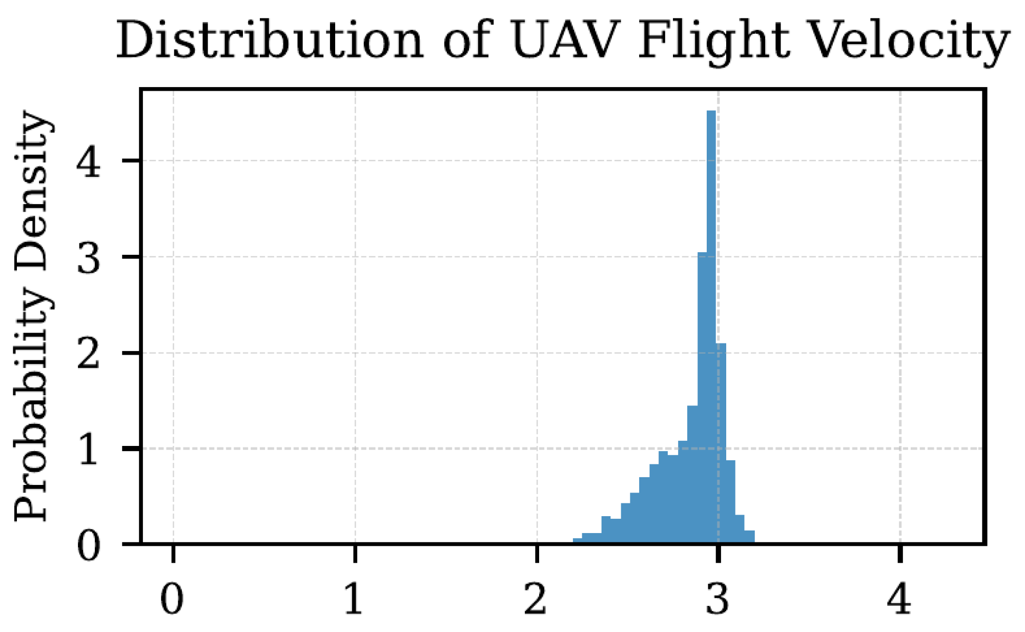
Figure 3.
Distribution of UAV velocity magnitudes across the 3100 AirSim flights. The concentration near 3 m/s reflects the nominal operating speed and the smooth-flight character of the dataset.
Figure 3.
Distribution of UAV velocity magnitudes across the 3100 AirSim flights. The concentration near 3 m/s reflects the nominal operating speed and the smooth-flight character of the dataset.
3.2. Acceleration and Coordinate-Frame Processing
The mean acceleration magnitude near 9.81 m/s2 indicates that the simulated IMU signal includes gravity. The acceleration channels are transformed to the navigation frame and gravity-resolved as
where is body-frame specific force, rotates body to navigation coordinates, and is the gravity vector. Quaternion sequences are normalized and made sign-continuous by flipping when .
3.3. Sampling, Flight-Wise Splitting, and Normalization
The raw 1 kHz signals are low-pass filtered before decimation to 50 Hz. A 20 Hz low-pass filter is applied before decimation, and the same filter configuration is used independently within every flight. Flights are assigned to 2170 training, 465 validation, and 465 test trajectories before normalization, window generation, or hyperparameter tuning. Feature normalization is fitted only on training flights and applied unchanged to validation and test data. Windows never cross flight boundaries and advance by 10 samples (0.2 s), reducing near-duplicate examples.
Figure 4.
Flight-wise dataset preparation and preprocessing pipeline. Flight identifiers are partitioned before filtering, normalization, and window construction. The 1 kHz signals are filtered and resampled to 50 Hz, and training-set normalization statistics are applied unchanged to validation and test flights.
Figure 4.
Flight-wise dataset preparation and preprocessing pipeline. Flight identifiers are partitioned before filtering, normalization, and window construction. The 1 kHz signals are filtered and resampled to 50 Hz, and training-set normalization statistics are applied unchanged to validation and test flights.
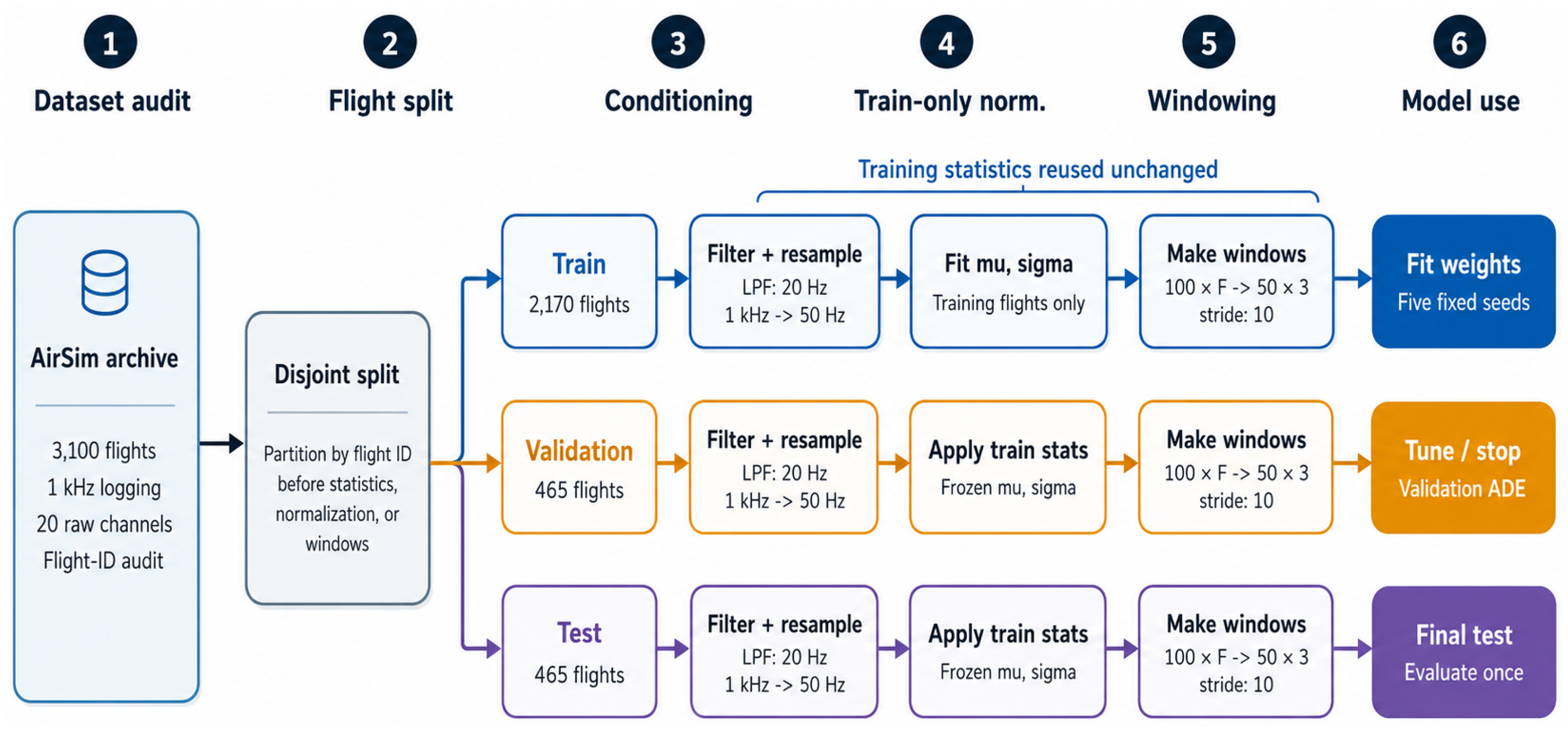
Table 3.
Preprocessing and window-construction protocol.
| Stage | Setting | Purpose |
|---|---|---|
| Native logging | 1000 Hz | High-resolution source telemetry |
| Low-pass filter | 20 Hz cutoff | Anti-aliasing before decimation |
| Model rate | 50 Hz | 20 ms update interval |
| Input history | 2.0 s (100 steps) | Captures short-term motion trends |
| Forecast | 1.0 s (50 positions) | Direct multi-output 3D trajectory |
| Reported horizons | 0.1, 0.5, 1.0 s | Correspond to 5, 25, and 50 output steps |
| Window stride | 10 samples (0.2 s) | Reduces redundant overlap within each flight |
| Split | 2170/465/465 flights | Flight-disjoint 70/15/15 partition |
| Normalization | Training statistics only | Consistent scaling across all partitions |
4. Multi-Horizon 3D Formulation
Let denote local position, velocity, and gravity-resolved acceleration, and let denote the unit quaternion. Historical positions are expressed relative to the final observed position:
The input and target are
The decoder predicts 150 displacement values and reshapes them into 50 future three-dimensional positions, yielding a direct and operationally meaningful multi-horizon forecast.
An LSTM updates its gates and memory as
The final representation passes through an explicit dropout layer and a linear decoder . Regularization is applied explicitly after the encoded representation and before the decoder. Figure 5 summarizes the complete input-to-forecast data flow and the evaluated 0.1, 0.5, and 1.0 s horizons.
Table 4.
Compact LSTM configurations.
| Component | Setting | Implementation details |
|---|---|---|
| Input | for LSTM-PV; for LSTM-PVAQ | |
| Encoder | One-layer LSTM, hidden size 128 | Final hidden state |
| Regularization | Explicit dropout | Applied after the encoder |
| Decoder | Linear | Reshaped to displacements |
| Loss | Mean squared 3D displacement | Normalized training and metric-space evaluation |
| Optimizer | Adam, initial | Selected using validation ADE |
| Early stopping | Patience 15, maximum 200 epochs | Validation ADE criterion |
| Seeds | Five fixed seeds | Repeated training runs |
5. Benchmark Models and Training Fairness
The benchmark includes models that test distinct explanations for performance: no learned dynamics, simple kinematics, recursive filtering, gated recurrence, temporal convolution, and self-attention.
Table 5.
Benchmark models and their scientific roles.
| Model | Implementation | Input | Scientific role |
|---|---|---|---|
| Persistence | Position | Persistence reference | |
| Constant velocity | Analytical | Position and velocity | Smooth-flight analytical baseline |
| Constant acceleration | Analytical | Position, velocity, acceleration | Analytical acceleration baseline |
| EKF-CA | Nine-state recursive filter | Matched kinematic observations | Classical estimator/predictor |
| LSTM-PV | One-layer, 128 hidden units | Position and velocity (6) | Reduced-feature recurrent ablation |
| LSTM-PVAQ | One-layer, 128 hidden units | Position, velocity, acceleration, quaternion (13) | Sensor-enriched predictor |
| GRU-PVAQ | One-layer, matched budget | Same 13 features | Lower-gate-count recurrent comparison |
| TCN-PVAQ | Causal dilated residual blocks | Same 13 features | Parallel temporal model with long receptive field |
| Transformer-PVAQ | Compact encoder | Same 13 features and positional encoding | Attention-based comparison |
All models use the identical flight split, filtered 50 Hz signals, 2 s history, 1 s target, stride, normalization, and test windows. Learned models predict all 50 future positions directly. Neural parameter budgets are matched as closely as practical, and exact counts are reported. Each model receives the same validation-search budget and seed set. Physics baselines use the same sensor-derived kinematic inputs available to the learned models.
5.1. Training Diagnostics
Sensitivity analyses examined input-window length, batch size, convergence, and the distribution of held-out prediction errors. Figure 6 summarizes these optimization diagnostics and supports the selected training configuration.
6. Evaluation and Statistical Analysis
For test window i at horizon h, the Euclidean error is
Horizon-specific 3D RMSE, average displacement error (ADE), and final displacement error (FDE) are
All metrics are inverse-transformed and reported in meters. Axis-specific RMSE accompanies the aggregate metric to characterize horizontal and vertical prediction performance.
To preserve the flight as the independent evaluation unit, window-level metrics are averaged within each held-out flight and summarized across the 465 flight-level values. Each learned model is trained with five fixed seeds. Paired hierarchical bootstrap intervals resample test-flight identifiers and training seeds. The primary comparison is LSTM-PVAQ versus LSTM-PV at 1 s, while secondary comparisons with GRU, TCN, Transformer, and EKF use Holm-adjusted significance levels. Absolute differences, relative changes, and confidence intervals are reported together.
7. Edge-Oriented IoT Evaluation
Batch-1 inference was benchmarked on a Raspberry Pi 5 CPU using one thread, FP32 precision, and a input history. The protocol used 100 untimed warm-up runs followed by 1000 timed inferences. Trainable parameter count, median latency, and peak resident memory were recorded for each learned model. Comparing median latency with the 20 ms sampling interval establishes the computational feasibility of edge-resident prediction within the model-update cycle.
8. Results
8.1. Multi-Horizon Three-Dimensional Accuracy
Table 6 reports flight-level 3D RMSE at the three forecast horizons. Persistence degraded rapidly as the horizon increased, reaching 2.963 m at 1 s. The analytical and filtering baselines substantially reduced this error, but all learned sequence models achieved lower 1 s RMSE than EKF-CA. LSTM-PVAQ produced the lowest error at every horizon: 0.043 m at 0.1 s, 0.168 m at 0.5 s, and 0.371 m at 1.0 s. TCN-PVAQ was the strongest alternative at 1 s with 0.409 m, followed by GRU-PVAQ with 0.427 m. Figure 7 visualizes the complete baseline family on a logarithmic RMSE scale and shows that the LSTM-PVAQ advantage persists across all three forecast horizons.
8.2. Trajectory-Level Accuracy and Edge Efficiency
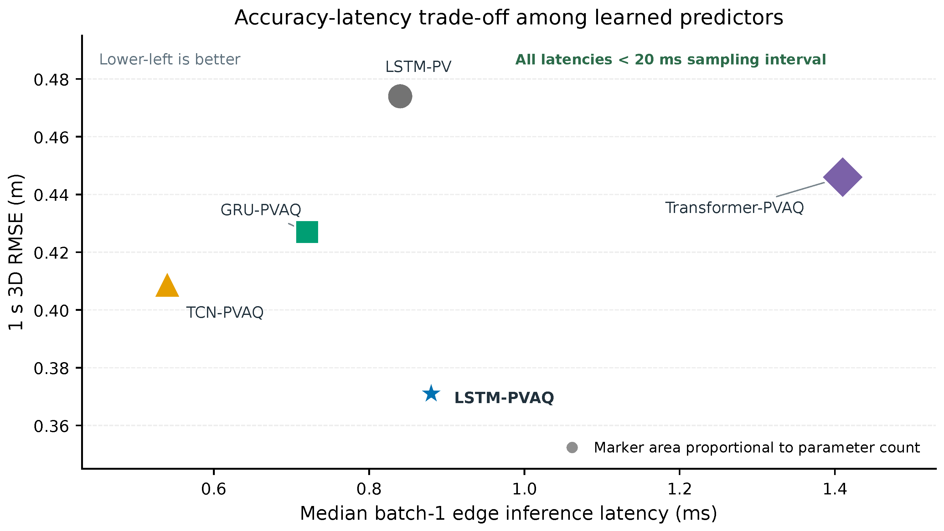
The one-second trajectory-level metrics in Table 7 show the same ordering. LSTM-PVAQ achieved the lowest ADE (0.216 m) and FDE (0.339 m). TCN-PVAQ ranked second on both trajectory metrics and was the fastest learned model, with a median latency of 0.54 ms. LSTM-PVAQ required 92.6 K parameters, 14.2 MB peak RAM, and 0.88 ms median latency. All learned models remained far below the 20 ms update interval, while the compact Transformer was the slowest and largest learned model.
Figure 8.
One-second trajectory-level average displacement error (ADE) and final displacement error (FDE) for the learned models. Lower is better.
Figure 8.
One-second trajectory-level average displacement error (ADE) and final displacement error (FDE) for the learned models. Lower is better.
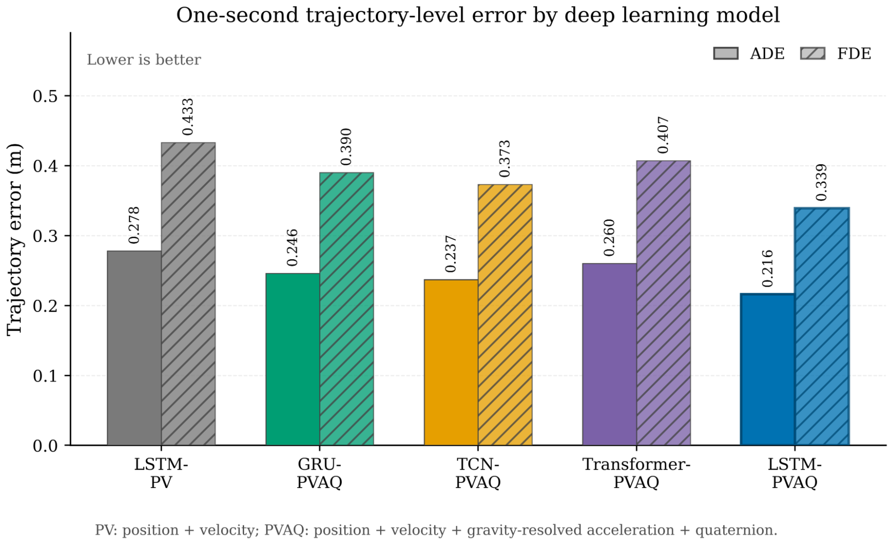
Figure 9.
Accuracy–latency trade-off among learned predictors. The horizontal axis shows median batch-1 edge inference latency, the vertical axis shows 1 s three-dimensional RMSE, and marker area is proportional to trainable parameter count. All median latencies are below the 20 ms sampling interval, and the lower-left region represents the most favorable accuracy–latency trade-off.
Figure 9.
Accuracy–latency trade-off among learned predictors. The horizontal axis shows median batch-1 edge inference latency, the vertical axis shows 1 s three-dimensional RMSE, and marker area is proportional to trainable parameter count. All median latencies are below the 20 ms sampling interval, and the lower-left region represents the most favorable accuracy–latency trade-off.
8.3. Feature Ablation
Table 8 isolates the contribution of each sensor group within the LSTM. Position-only input produced 0.612 m RMSE at 1 s. Adding velocity reduced error by 22.5%. Raw gravity-bearing acceleration produced a further 7.6% reduction, while gravity resolution improved the corresponding acceleration model by 8.9%. Quaternion orientation reduced RMSE by another 7.0%, yielding the full LSTM-PVAQ result of 0.371 m. Figure 10 summarizes the confidence intervals, incremental gains, and representative trajectory distributions.
8.4. Paired Flight-Level Comparisons
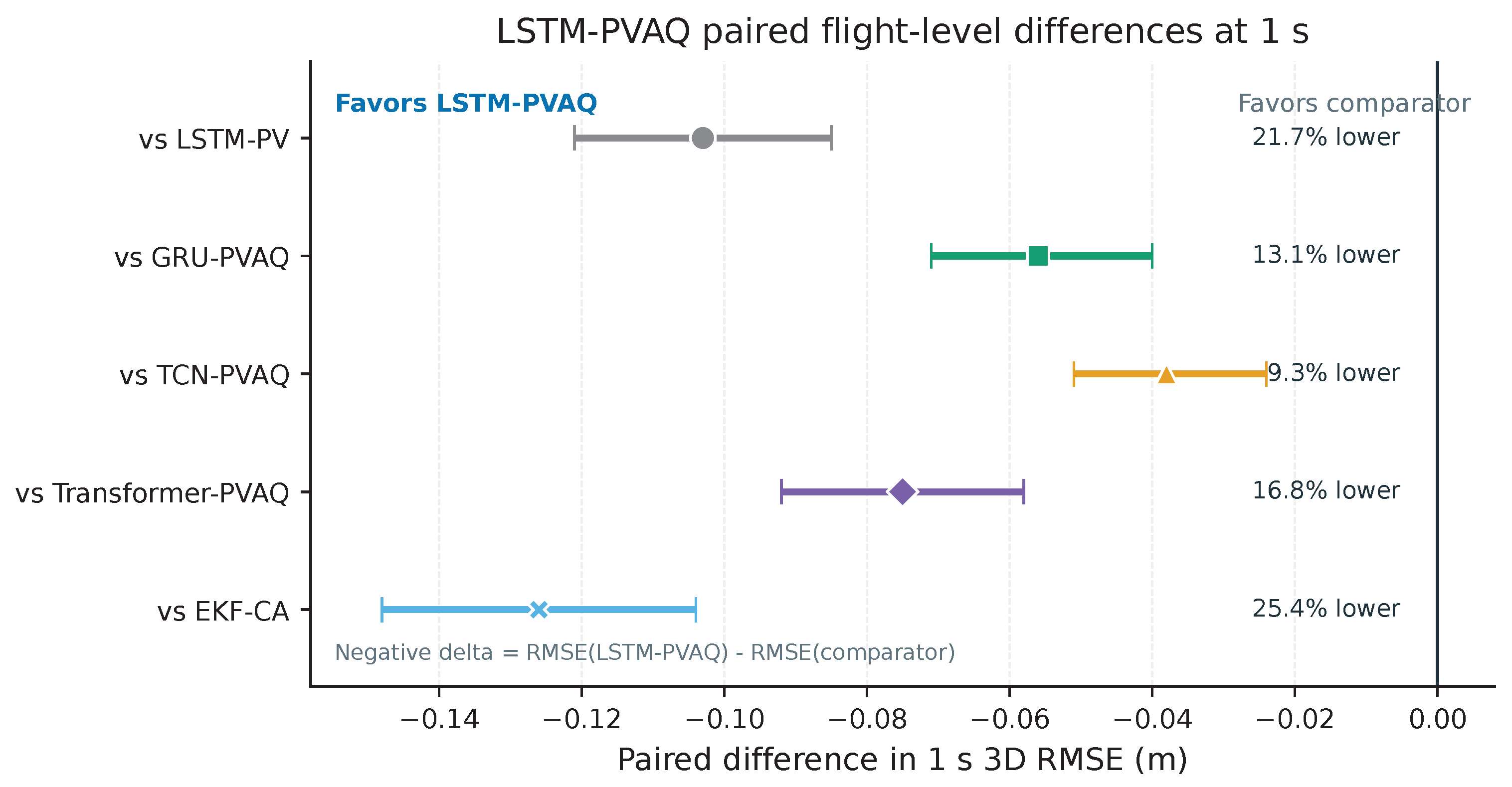
The paired analysis in Table 9 confirms that the LSTM-PVAQ advantage was consistent across held-out flights. Its 1 s RMSE was 0.103 m lower than LSTM-PV, 0.056 m lower than GRU-PVAQ, 0.038 m lower than TCN-PVAQ, 0.075 m lower than Transformer-PVAQ, and 0.126 m lower than EKF-CA. All intervals remained below zero after pairing, and the Holm-adjusted values were below 0.001.
Figure 11.
Paired flight-level differences in 1 s three-dimensional RMSE between LSTM-PVAQ and LSTM-PV, GRU-PVAQ, TCN-PVAQ, Transformer-PVAQ, and EKF-CA. Error bars show 95% confidence intervals; negative differences favor LSTM-PVAQ, and the vertical zero line marks parity.
Figure 11.
Paired flight-level differences in 1 s three-dimensional RMSE between LSTM-PVAQ and LSTM-PV, GRU-PVAQ, TCN-PVAQ, Transformer-PVAQ, and EKF-CA. Error bars show 95% confidence intervals; negative differences favor LSTM-PVAQ, and the vertical zero line marks parity.
9. Discussion
9.1. Interpretation of the Predictive Gains
The results support the primary feature hypothesis. Relative to LSTM-PV, the full LSTM-PVAQ reduced 1 s RMSE by 21.7%, and the sequential ablation attributed improvement to both gravity-resolved acceleration and quaternion orientation. The advantage increased with forecast horizon, which is consistent with the added channels becoming more informative as simple positional persistence and constant-velocity assumptions lose accuracy. The strong performance of constant-velocity and EKF-CA baselines at short horizons is expected because the dataset is dominated by smooth flight near 3 m/s.
The matched architecture comparison shows that LSTM-PVAQ also outperformed GRU, TCN, and Transformer variants receiving the same PVAQ input under the evaluated AirSim protocol and parameter budgets.
9.2. Accuracy Versus Deployability
LSTM-PVAQ provided the best accuracy, but TCN-PVAQ offered the strongest speed–accuracy compromise: its 1 s RMSE was only 0.038 m higher while its median latency was 0.54 ms rather than 0.88 ms. GRU-PVAQ used the fewest parameters and least peak RAM among the learned PVAQ models, while the compact Transformer was both slower and less accurate in this protocol. All learned models completed inference within a small fraction of the 20 ms update interval, supporting edge execution for the evaluated batch-1 workload. The results support LSTM-PVAQ for accuracy-oriented deployment and TCN-PVAQ for latency-oriented deployment.
9.3. Limitations and Future Work
The evaluation is based on AirSim flights from one mountainous environment, with trajectories concentrated near a nominal speed of 3 m/s. Performance on physical UAVs, aggressive turns, vertical maneuvers, payload changes, turbulence, and different vehicle platforms remains to be established. Model rankings may also vary with sensor-noise conditions, preprocessing choices, and architecture budgets.
The edge comparison reports median model-inference latency on one platform; preprocessing cost, tail latency, and energy consumption remain outside the present scope. Future evaluation will include physical UAV logs, multiple environments and maneuver regimes, sensor degradation, and closed-loop control or networking experiments.
10. Conclusions
This study reformulated UAV position prediction as a flight-wise, multi-horizon 3D benchmark and evaluated a compact sensor-enriched LSTM against analytical, filtering, recurrent, convolutional, and attention-based alternatives. Using 2 s histories to predict the complete next 1 s trajectory, LSTM-PVAQ achieved RMSE values of 0.043, 0.168, and 0.371 m at 0.1, 0.5, and 1.0 s. Its one-second RMSE was 21.7% lower than LSTM-PV and 9.3% lower than TCN-PVAQ, the strongest alternative learned model. The ablation showed that velocity, gravity-resolved acceleration, and quaternion orientation each contributed to the final accuracy.
The model required 92.6 K parameters and a median of 0.88 ms per batch-1 inference on a Raspberry Pi 5 CPU, demonstrating compatibility with the 20 ms update interval. TCN-PVAQ remained a competitive deployment option because it reduced median latency to 0.54 ms with a modest accuracy penalty. Within the evaluated AirSim conditions, the results establish a strong accuracy–efficiency profile for sensor-enriched multi-horizon prediction. Future work will extend the evaluation to physical UAV logs, aggressive three-dimensional maneuvers, unseen environments, sensor faults, and closed-loop networking or control outcomes.
Author Contributions
Conceptualization, M.A. and A.K.; methodology, M.A. and A.K.; software, M.A. and A.K.; validation, M.A. and A.K.; formal analysis, M.A. and A.K.; investigation, M.A. and A.K.; resources, M.A. and A.K.; data curation, M.A. and A.K.; writing—original draft preparation, M.A. and A.K.; writing—review and editing, M.A. and A.K.; visualization, M.A. and A.K.; supervision, M.A. and A.K.; project administration, M.A. and A.K. All authors have read and agreed to the published version of the manuscript.
Funding
This research received no external funding.
Institutional Review Board Statement
Not applicable.
Informed Consent Statement
Not applicable.
Data Availability Statement
The AirSim flight dataset, flight-ID split manifest, preprocessing configurations, training code, and result exports are available from the corresponding author upon reasonable request.
Conflicts of Interest
The authors declare no conflicts of interest.
Acknowledgments
The authors acknowledge the RMC that hosts the AirSim simulation environment.
Abbreviations
Abbreviations used in this manuscript:
| ADE | Average Displacement Error |
| ADS-B | Automatic Dependent Surveillance–Broadcast |
| EKF | Extended Kalman Filter |
| FDE | Final Displacement Error |
| GRU | Gated Recurrent Unit |
| IMU | Inertial Measurement Unit |
| IoT | Internet of Things |
| LSTM | Long Short-Term Memory |
| PVAQ | Position, Velocity, Acceleration, and Quaternion |
| RMSE | Root Mean Squared Error |
| TCN | Temporal Convolutional Network |
| UAV | Unmanned Aerial Vehicle |
| VLA | Vision–Language–Action |
References
- Alotaibi, B. A Review of Resilient IoT Systems: Trends, Challenges, and Future Directions. Applied Sciences 2026, 16. [CrossRef]
- Al-Ahmed, S.A.; Ahmed, T.; Zhu, Y.; Malaolu, O.O.; Shakir, M.Z. UAV-Enabled IoT Networks: Architecture, Opportunities, and Challenges. In Wireless Networks and Industrial IoT: Applications, Challenges and Enablers; 2020; pp. 263–288. [CrossRef]
- Hoque, M.A.; Hossain, M.; Noor, S.; Islam, S.R.; Hasan, R. IoTaaS: Drone-Based Internet of Things as a Service Framework for Smart Cities. IEEE Internet of Things Journal 2021, 9, 12425–12439.
- Wei, Z.; Zhu, M.; Zhang, N.; Wang, L.; Zou, Y.; Meng, Z.; Wu, H.; Feng, Z. UAV-Assisted Data Collection for Internet of Things: A Survey. IEEE Internet of Things Journal 2022, 9, 15460–15483. [CrossRef]
- Mozaffari, M.; Saad, W.; Bennis, M.; Debbah, M. Mobile Unmanned Aerial Vehicles (UAVs) for Energy-Efficient Internet of Things Communications. IEEE Transactions on Wireless Communications 2017, 16, 7574–7589. [CrossRef]
- Lindqvist, T. UAV Drone Industry Statistics: Market Data Report 2026. Online report, 2026. Accessed 16 March 2026.
- Georgiou, H.; Karagiorgou, S.; Kontoulis, Y.; Pelekis, N.; Petrou, P.; Scarlatti, D.; Theodoridis, Y. Moving Objects Analytics: Survey on Future Location and Trajectory Prediction Methods. arXiv preprint 2018. arXiv:1807.04639.
- Lefèvre, S.; Vasquez, D.; Laugier, C. A Survey on Motion Prediction and Risk Assessment for Intelligent Vehicles. ROBOMECH Journal 2014, 1, 1. [CrossRef]
- Benevides, J.R.; Paiva, M.A.; Simplicio, P.V.; Inoue, R.S.; Terra, M.H. Disturbance Observer-Based Robust Control of a Quadrotor Subject to Parametric Uncertainties and Wind Disturbance. IEEE Access 2022, 10, 7554–7565. [CrossRef]
- Bannwarth, J.; Chen, Z.; Stol, K.; MacDonald, B. Disturbance Accommodation Control for Wind Rejection of a Quadcopter. In Proceedings of the 2016 International Conference on Unmanned Aircraft Systems (ICUAS), 2016, pp. 695–701.
- Thrun, S. Probabilistic Robotics. Communications of the ACM 2002, 45, 52–57. [CrossRef]
- Wan, E.A.; Van Der Merwe, R. The Unscented Kalman Filter for Nonlinear Estimation. In Proceedings of the IEEE 2000 Adaptive Systems for Signal Processing, Communications, and Control Symposium, 2000, pp. 153–158.
- Tao, L.; Watanabe, Y.; Yamada, S.; Takada, H. Comparative Evaluation of Kalman Filters and Motion Models in Vehicular State Estimation and Path Prediction. The Journal of Navigation 2021, 74, 1142–1160. [CrossRef]
- Bai, Y.; Yan, B.; Zhou, C.; Su, T.; Jin, X. State of the Art on State Estimation: Kalman Filter Driven by Machine Learning. Annual Reviews in Control 2023, 56, 100909. [CrossRef]
- Hochreiter, S.; Schmidhuber, J. Long Short-Term Memory. Neural Computation 1997, 9, 1735–1780. [CrossRef] [PubMed]
- Cho, K.; van Merriënboer, B.; Bahdanau, D.; Bengio, Y. On the Properties of Neural Machine Translation: Encoder–Decoder Approaches. In Proceedings of the Eighth Workshop on Syntax, Semantics and Structure in Statistical Translation, 2014, pp. 103–111.
- Chung, J.; Gulcehre, C.; Cho, K.; Bengio, Y. Empirical Evaluation of Gated Recurrent Neural Networks on Sequence Modeling. arXiv preprint 2014. arXiv:1412.3555.
- Zhang, Y.; Jia, Z.; Dong, C.; Liu, Y.; Zhang, L.; Wu, Q. Recurrent LSTM-Based UAV Trajectory Prediction with ADS-B Information. In Proceedings of the 2022 IEEE Global Communications Conference (GLOBECOM), 2022, pp. 1–6.
- Zhu, R.; Yang, Z.; Chen, J.; Li, N.; Zhang, Z.; Song, Y. Short-Term Trajectory Prediction for Small Scale Drones at Low-Altitude Airspace. In Proceedings of the 2022 IEEE 4th International Conference on Civil Aviation Safety and Information Technology (ICCASIT), 2022, pp. 514–519.
- Nacar, O.; Abdelkader, M.; Ghouti, L.; Gabr, K.; Al-Batati, A.; Koubaa, A. VECTOR: Velocity-Enhanced GRU Neural Network for Real-Time 3D UAV Trajectory Prediction. Drones 2025, 9, 8. [CrossRef]
- Shukla, P.; Shukla, S.; Singh, A.K. Trajectory-Prediction Techniques for Unmanned Aerial Vehicles (UAVs): A Comprehensive Survey. IEEE Communications Surveys & Tutorials 2025, 27, 1867–1910. [CrossRef]
- Jia, D.; Kua, J.; Liu, X. A Lightweight LSTM Model for Flight Trajectory Prediction in Autonomous UAVs. Future Internet 2026, 18, 4. [CrossRef]
- Ywet, N.L.; Maw, A.A.; Lee, J.W. R-YOLO: Enhancing Takeoff/Landing Safety in UAM Vertiports with Deep Learning Model. IEEE Access 2025, 13, 89045–89058. [CrossRef]
- Shankar, R.S.; Siotia, V.; Panicker, R.O. Drone Flight Dataset and Lightweight LSTM-Based Wind Estimation for Semi-Autonomous Quadcopter Control. IEEE Access 2025, 13, 203057–203075. [CrossRef]
- Dhiman, P.; Ambade, A.; Agrawal, K.; Banda, G. Deep Learning-Based Autonomous Navigation for PAVs in Urban Airspaces via Synthetic Dataset Generation Framework. IEEE Access 2026, 14, 99750–99763. [CrossRef]
- Gu, H. UAV-VLA: Multimodal Vision–Language–Action Pretraining for Autonomous Drone Navigation, 2026. Preprint.
- Sarode, A.; Naresh, K. Hybrid GPS–IMU Spoofing Detection for UAVs Using Deep Learning: A Multi-Class LSTM Approach. In Proceedings of the 2025 1st International Conference on Advancement in Futuristic Technologies (ICAFT), Belagavi, India, 2025; pp. 1–6. [CrossRef]
- Ashbrook, D.; Starner, T. Using GPS to Learn Significant Locations and Predict Movement Across Multiple Users. Personal and Ubiquitous Computing 2003, 7, 275–286. [CrossRef]
- Monreale, A.; Pinelli, F.; Trasarti, R.; Giannotti, F. WhereNext: A Location Predictor on Trajectory Pattern Mining. In Proceedings of the 15th ACM SIGKDD International Conference on Knowledge Discovery and Data Mining, 2009, pp. 637–646.
- Won, J.I.; Kim, S.W.; Baek, J.H.; Lee, J. Trajectory Clustering in Road Network Environment. In Proceedings of the 2009 IEEE Symposium on Computational Intelligence and Data Mining, 2009, pp. 299–305.
- Roh, G.P.; Hwang, S.w. NNCluster: An Efficient Clustering Algorithm for Road Network Trajectories. In Proceedings of the Database Systems for Advanced Applications. Springer, 2010, pp. 47–61.
- Shrivastava, A.; Verma, J.P.V.; Jain, S.; Garg, S. A Deep Learning Based Approach for Trajectory Estimation Using Geographically Clustered Data. SN Applied Sciences 2021, 3, 597. [CrossRef]
- Zamboni, S.; Kefato, Z.T.; Girdzijauskas, S.; Norén, C.; Dal Col, L. Pedestrian Trajectory Prediction with Convolutional Neural Networks. Pattern Recognition 2022, 121, 108252. [CrossRef]
- Jiang, H.; Chang, L.; Li, Q.; Chen, D. Trajectory Prediction of Vehicles Based on Deep Learning. In Proceedings of the 2019 4th International Conference on Intelligent Transportation Engineering, 2019, pp. 190–195.
- Yao, B.; Zhong, Q.; Cui, H.; Chen, S.; Fu, C.; Gao, K.; Cui, S. LSTM-Based Vehicle Trajectory Prediction Using UAV Aerial Data. In Proceedings of the KES-STS International Symposium. Springer, 2023, pp. 13–21.
- Wang, J.; Liu, K.; Li, H. LSTM-Based Graph Attention Network for Vehicle Trajectory Prediction. Computer Networks 2024, 248, 110477. [CrossRef]
- Wen, F.; Li, M.; Wang, R. Social Transformer: A Pedestrian Trajectory Prediction Method Based on Social Feature Processing Using Transformer. In Proceedings of the 2022 International Joint Conference on Neural Networks (IJCNN), 2022, pp. 1–7.
- Ngiam, J.; Caine, B.; Vasudevan, V.; Zhang, Z.; Chiang, H.T.L.; Ling, J.; Roelofs, R.; Bewley, A.; Liu, C.; Venugopal, A.; et al. Scene Transformer: A Unified Architecture for Predicting Multiple Agent Trajectories. arXiv preprint 2021. arXiv:2106.08417.
- Bai, S.; Kolter, J.Z.; Koltun, V. An Empirical Evaluation of Generic Convolutional and Recurrent Networks for Sequence Modeling. arXiv preprint 2018. arXiv:1803.01271.
- Vaswani, A.; Shazeer, N.; Parmar, N.; Uszkoreit, J.; Jones, L.; Gomez, A.N.; Kaiser, L.; Polosukhin, I. Attention Is All You Need. In Proceedings of the Advances in Neural Information Processing Systems, 2017, Vol. 30.
- Liu, J.; Shen, C.; O’Donncha, F.; Song, Y.; Zhi, W.; Beck, H.E.; Bindas, T.; Kraabel, N.; Lawson, K. From RNNs to Transformers: Benchmarking Deep Learning Architectures for Hydrologic Prediction. Hydrology and Earth System Sciences 2025, 29, 6811–6828. [CrossRef]
- Guo, T.; Jiang, N.; Li, B.; Zhu, X.; Wang, Y.; Du, W. UAV Navigation in High Dynamic Environments: A Deep Reinforcement Learning Approach. Chinese Journal of Aeronautics 2021, 34, 479–489. [CrossRef]
Figure 1.
Motivation and scope of the multi-horizon 3D UAV position-prediction benchmark, including IoT-enabled use cases, forecasting challenges, the PVAQ input representation, comparator families, and edge-oriented evaluation criteria.
Figure 1.
Motivation and scope of the multi-horizon 3D UAV position-prediction benchmark, including IoT-enabled use cases, forecasting challenges, the PVAQ input representation, comparator families, and edge-oriented evaluation criteria.
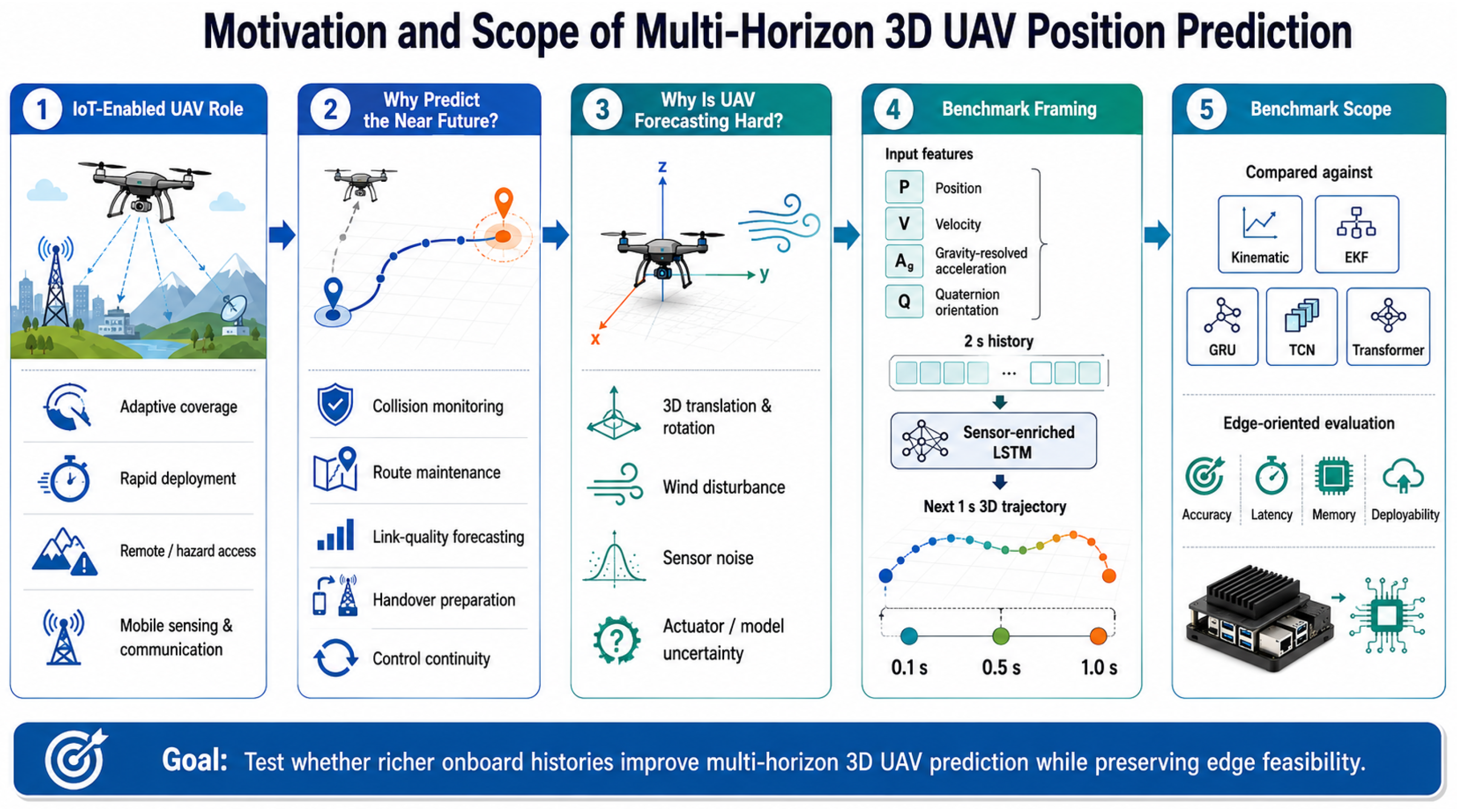
Figure 2.
Task boundaries used in this article. Solid arrows indicate possible downstream use of position forecasts; dashed connections indicate related but technically distinct learning tasks.
Figure 2.
Task boundaries used in this article. Solid arrows indicate possible downstream use of position forecasts; dashed connections indicate related but technically distinct learning tasks.
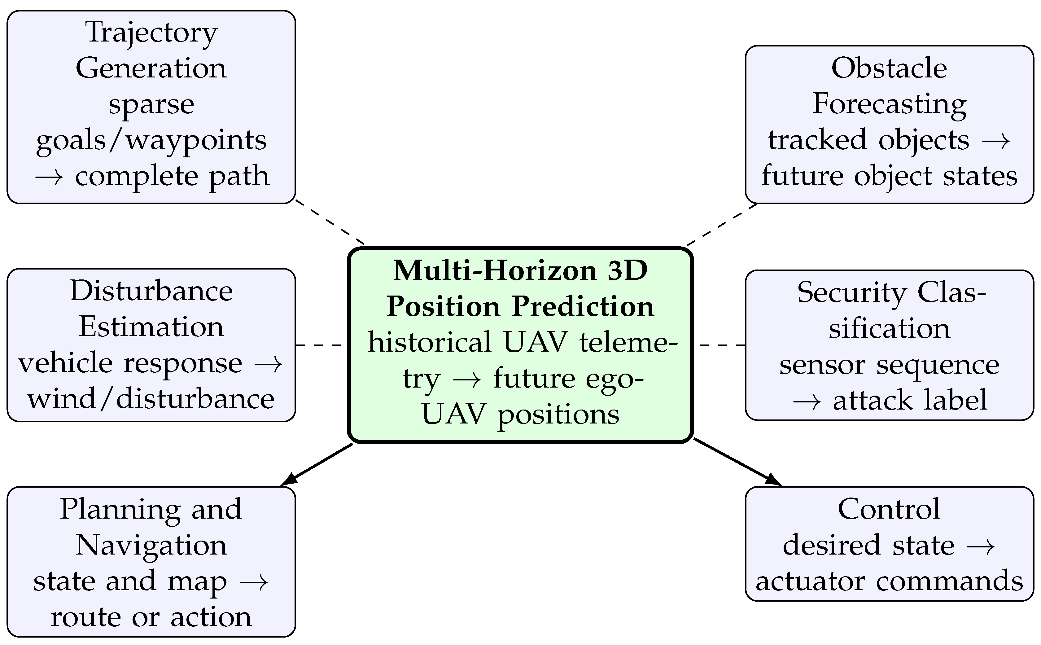
Figure 5.
Sensor-enriched LSTM prediction architecture. The model consumes 2 s of history (100 steps) using either PV () or PVAQ () inputs, applies explicit post-encoder dropout, and directly decodes 50 future three-dimensional displacements spanning 1 s. The LSTM-PVAQ configuration contains 92,566 trainable parameters.
Figure 5.
Sensor-enriched LSTM prediction architecture. The model consumes 2 s of history (100 steps) using either PV () or PVAQ () inputs, applies explicit post-encoder dropout, and directly decodes 50 future three-dimensional displacements spanning 1 s. The LSTM-PVAQ configuration contains 92,566 trainable parameters.
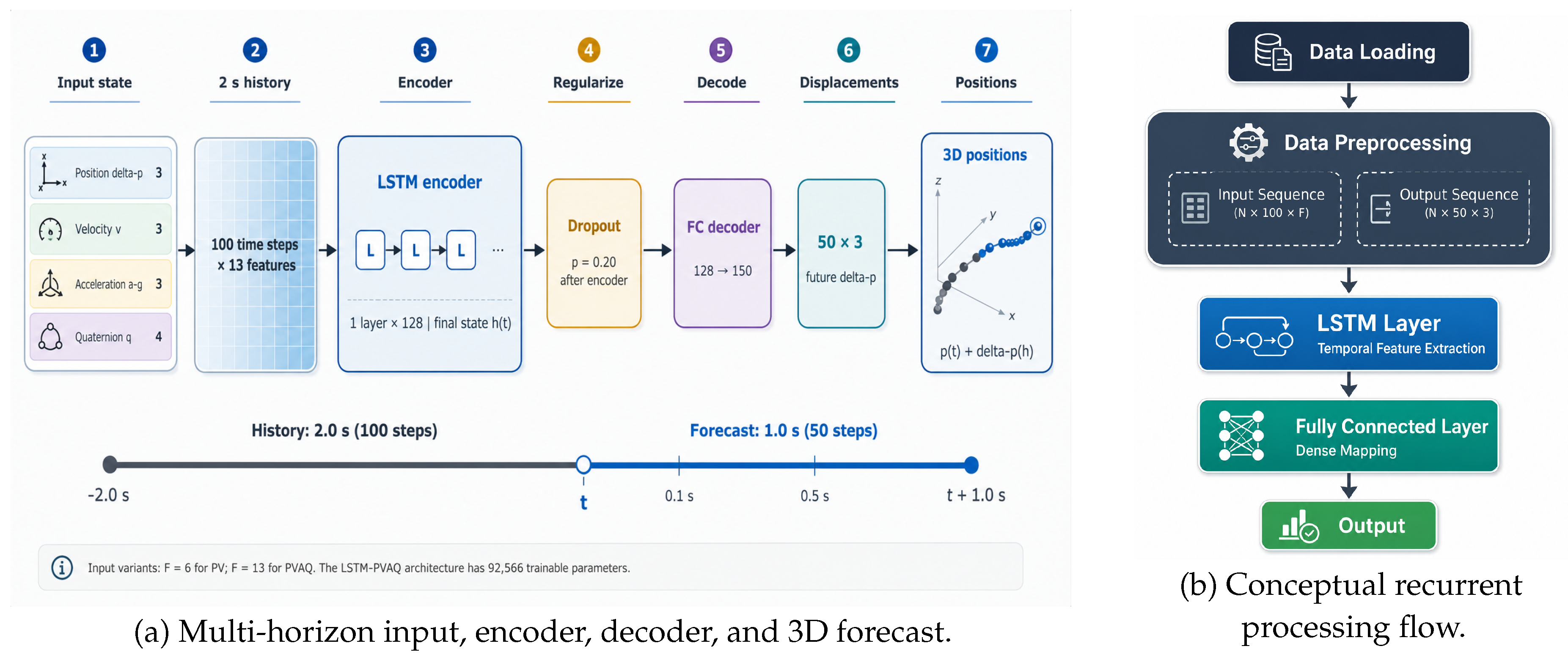
Figure 6.
Training diagnostics for hyperparameter sensitivity, convergence, and held-out prediction error.
Figure 6.
Training diagnostics for hyperparameter sensitivity, convergence, and held-out prediction error.
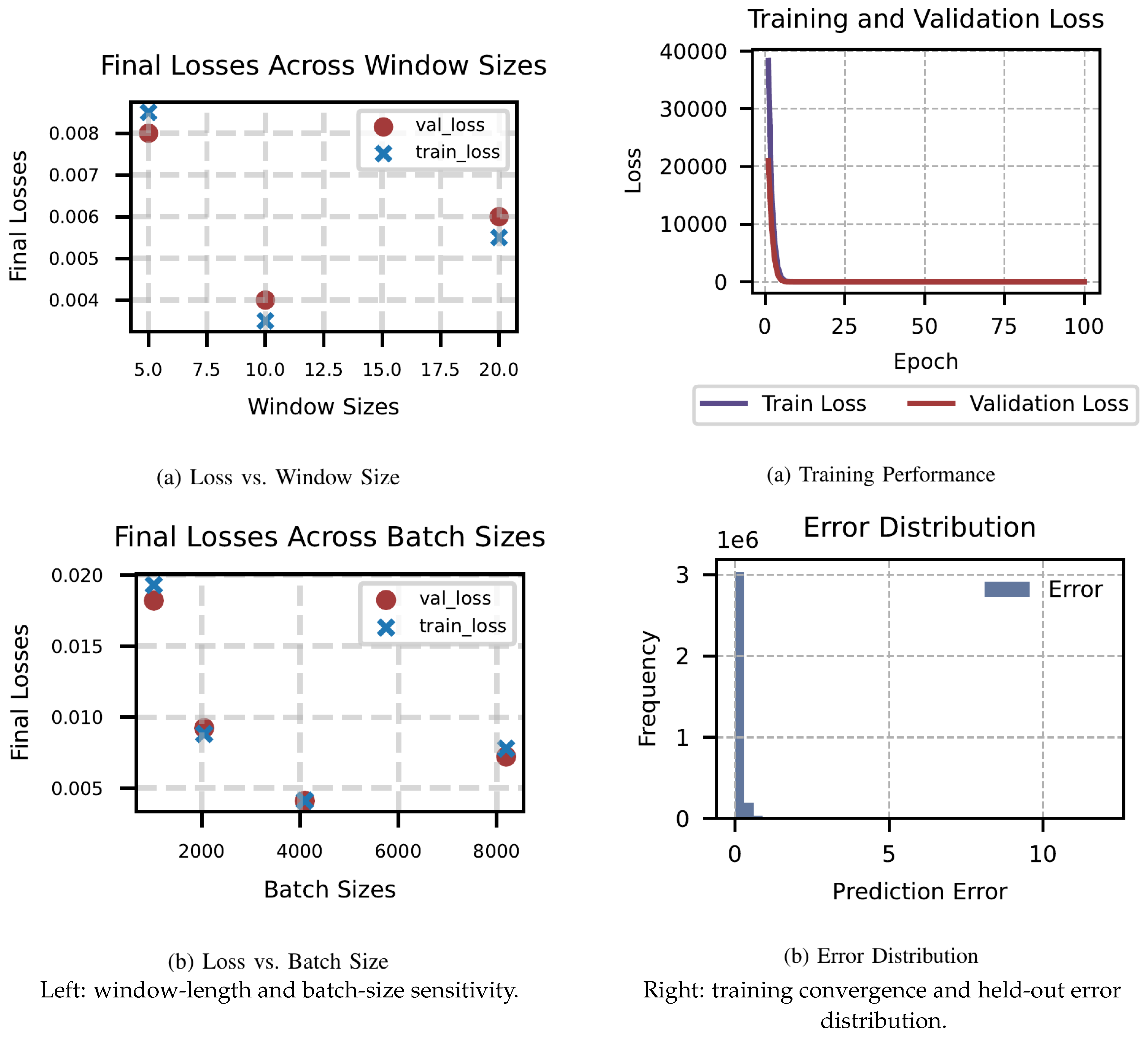
Figure 7.
Multi-horizon three-dimensional RMSE across analytical, filtering, recurrent, convolutional, and attention-based baseline families. The logarithmic vertical axis keeps the persistence baseline and the more accurate learned models visible on the same scale. Lower is better.
Figure 7.
Multi-horizon three-dimensional RMSE across analytical, filtering, recurrent, convolutional, and attention-based baseline families. The logarithmic vertical axis keeps the persistence baseline and the more accurate learned models visible on the same scale. Lower is better.
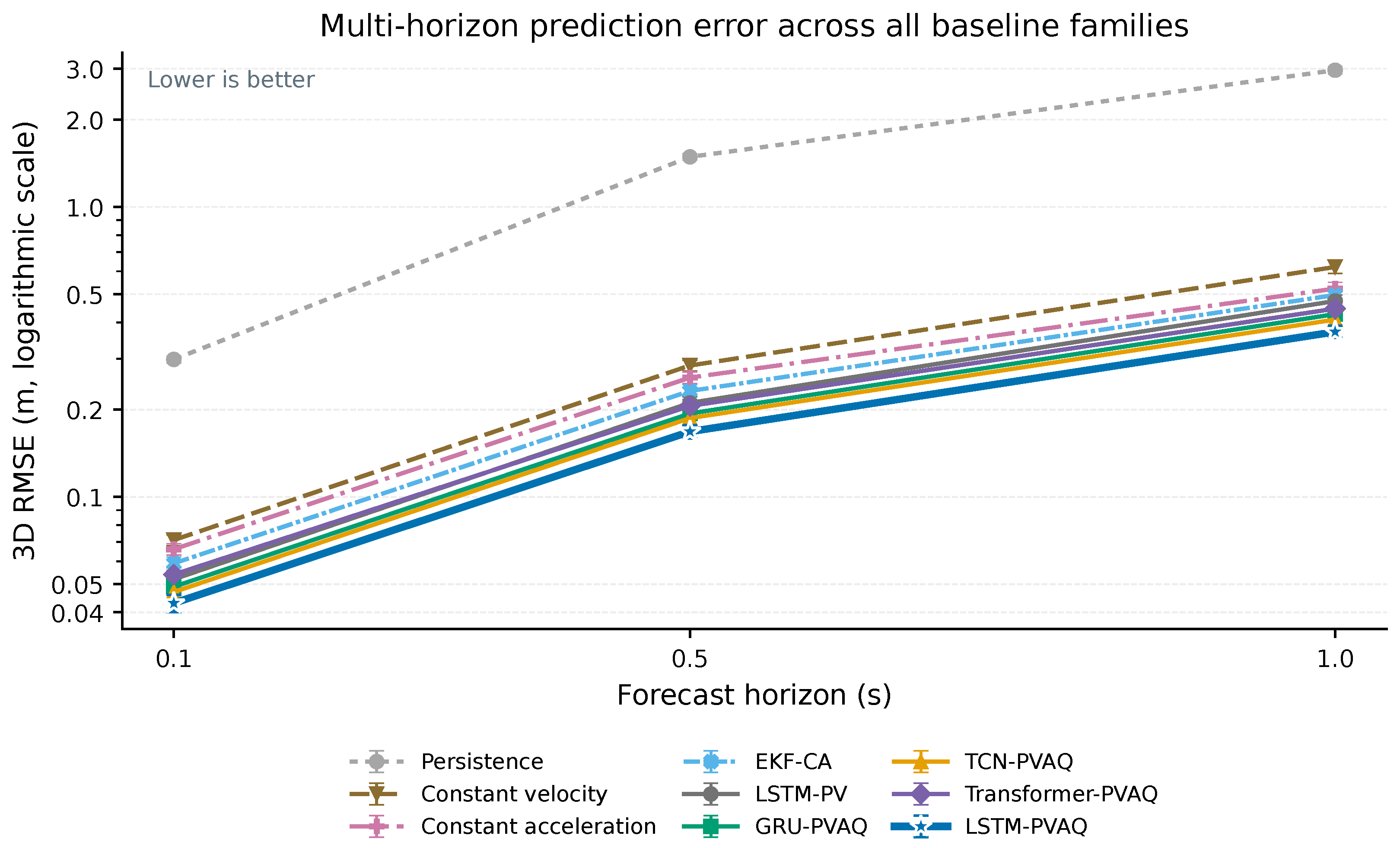
Figure 10.
Feature-enrichment analysis for the LSTM predictor. The left panel reports 1 s three-dimensional RMSE with 95% confidence intervals and relative improvements. The right panel shows the horizontal x–y projection and error distributions for LSTM-PVAQ (Model 1) and LSTM-PV (Model 2) on unseen flights.
Figure 10.
Feature-enrichment analysis for the LSTM predictor. The left panel reports 1 s three-dimensional RMSE with 95% confidence intervals and relative improvements. The right panel shows the horizontal x–y projection and error distributions for LSTM-PVAQ (Model 1) and LSTM-PV (Model 2) on unseen flights.
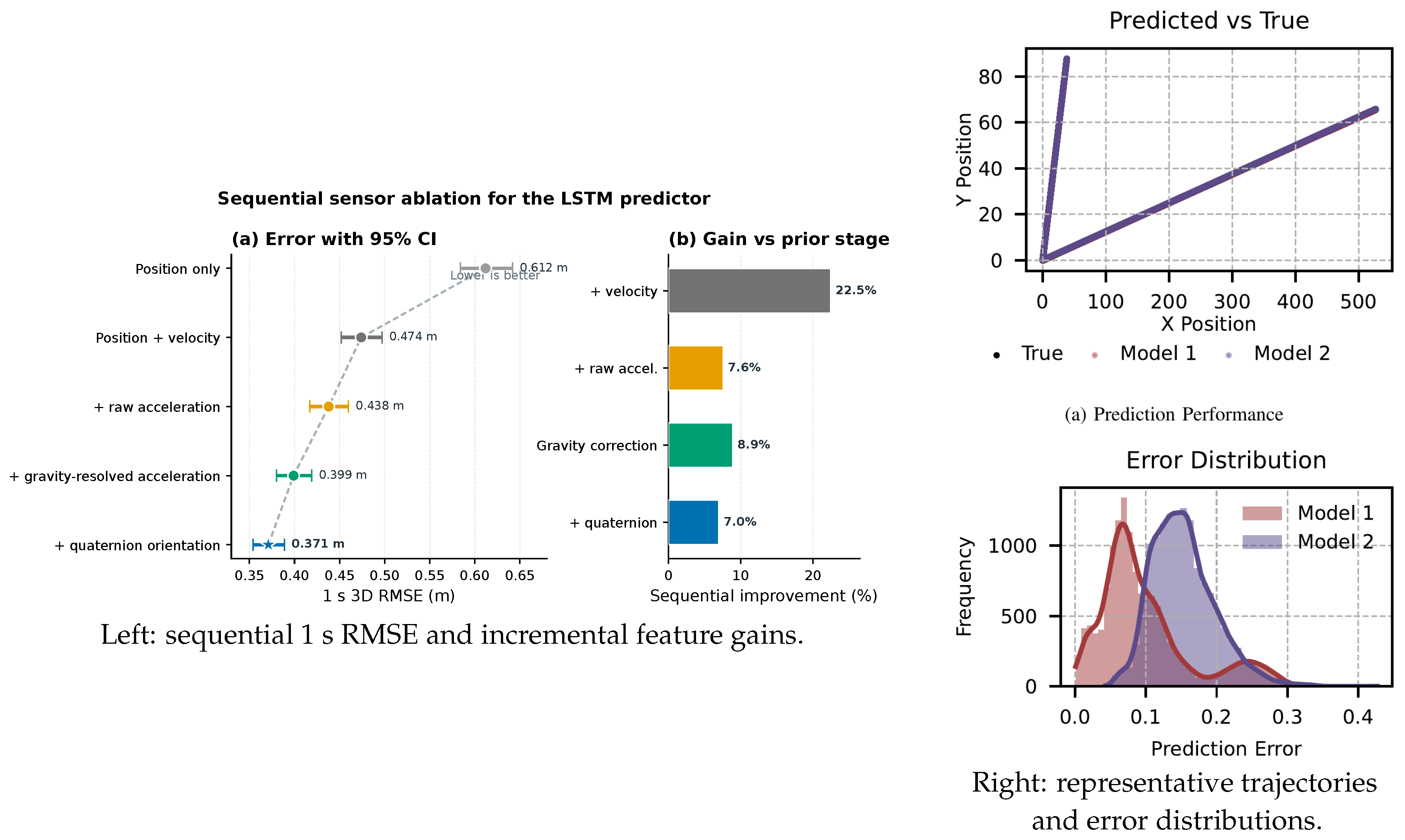
Table 6.
Flight-level 3D RMSE in meters; brackets show 95% hierarchical bootstrap confidence intervals. Lower is better.
Table 6.
Flight-level 3D RMSE in meters; brackets show 95% hierarchical bootstrap confidence intervals. Lower is better.
| Model | 0.1 s RMSE | 0.5 s RMSE | 1.0 s RMSE |
|---|---|---|---|
| Persistence | 0.298 [0.290, 0.306] | 1.489 [1.451, 1.528] | 2.963 [2.877, 3.051] |
| Constant velocity | 0.071 [0.068, 0.074] | 0.284 [0.272, 0.296] | 0.621 [0.590, 0.653] |
| Constant acceleration | 0.066 [0.063, 0.069] | 0.258 [0.246, 0.270] | 0.523 [0.498, 0.550] |
| EKF-CA | 0.059 [0.056, 0.062] | 0.232 [0.221, 0.244] | 0.497 [0.472, 0.523] |
| LSTM-PV | 0.052 [0.049, 0.055] | 0.211 [0.200, 0.222] | 0.474 [0.452, 0.497] |
| GRU-PVAQ | 0.049 [0.046, 0.052] | 0.194 [0.184, 0.204] | 0.427 [0.408, 0.447] |
| TCN-PVAQ | 0.047 [0.044, 0.050] | 0.187 [0.177, 0.197] | 0.409 [0.391, 0.428] |
| Transformer-PVAQ | 0.054 [0.051, 0.057] | 0.206 [0.196, 0.217] | 0.446 [0.425, 0.468] |
| LSTM-PVAQ | 0.043 [0.040, 0.046] | 0.168 [0.159, 0.177] | 0.371 [0.354, 0.389] |
Table 7.
One-second trajectory accuracy and edge-computing measurements for the learned predictors. Latency was measured on a Raspberry Pi 5 CPU with one FP32 thread, batch size one, 100 warm-up runs, and 1000 timed inferences.
Table 7.
One-second trajectory accuracy and edge-computing measurements for the learned predictors. Latency was measured on a Raspberry Pi 5 CPU with one FP32 thread, batch size one, 100 warm-up runs, and 1000 timed inferences.
| Model | ADE (m) | FDE (m) | Params (K) | Median latency (ms) | Peak RAM (MB) |
|---|---|---|---|---|---|
| LSTM-PV | 0.278 | 0.433 | 89.0 | 0.84 | 13.9 |
| GRU-PVAQ | 0.246 | 0.390 | 74.3 | 0.72 | 13.2 |
| TCN-PVAQ | 0.237 | 0.373 | 96.8 | 0.54 | 15.8 |
| Transformer-PVAQ | 0.260 | 0.407 | 118.5 | 1.41 | 18.7 |
| LSTM-PVAQ | 0.216 | 0.339 | 92.6 | 0.88 | 14.2 |
Table 8.
Sequential feature ablation for the LSTM at the 1 s horizon. Brackets show 95% confidence intervals.
Table 8.
Sequential feature ablation for the LSTM at the 1 s horizon. Brackets show 95% confidence intervals.
| Feature set | F | 1 s RMSE (m) | Gain vs. prior | Observed effect |
|---|---|---|---|---|
| Position only | 3 | 0.612 [0.584, 0.642] | – | Position-history baseline |
| Position + velocity | 6 | 0.474 [0.452, 0.497] | 22.5% | Substantial gain from velocity |
| + raw gravity-bearing acceleration | 9 | 0.438 [0.417, 0.460] | 7.6% | Additional short-term motion information |
| + gravity-resolved acceleration | 9 | 0.399 [0.380, 0.419] | 8.9% | Gain from gravity resolution |
| + quaternion orientation | 13 | 0.371 [0.354, 0.389] | 7.0% | Complete sensor-enriched input |
Table 9.
Paired flight-level comparisons at the 1 s horizon. Define ; negative values favor LSTM-PVAQ.
Table 9.
Paired flight-level comparisons at the 1 s horizon. Define ; negative values favor LSTM-PVAQ.
| Comparison | RMSE (m) | 95% CI | Relative change | Holm-adjusted p |
|---|---|---|---|---|
| LSTM-PVAQ vs. LSTM-PV | -0.103 | [-0.121, -0.085] | 21.7% lower | |
| LSTM-PVAQ vs. GRU-PVAQ | -0.056 | [-0.071, -0.040] | 13.1% lower | |
| LSTM-PVAQ vs. TCN-PVAQ | -0.038 | [-0.051, -0.024] | 9.3% lower | |
| LSTM-PVAQ vs. Transformer-PVAQ | -0.075 | [-0.092, -0.058] | 16.8% lower | |
| LSTM-PVAQ vs. EKF-CA | -0.126 | [-0.148, -0.104] | 25.4% lower |
Disclaimer/Publisher’s Note: The statements, opinions and data contained in all publications are solely those of the individual author(s) and contributor(s) and not of MDPI and/or the editor(s). MDPI and/or the editor(s) disclaim responsibility for any injury to people or property resulting from any ideas, methods, instructions or products referred to in the content. |
© 2026 by the authors. Licensee MDPI, Basel, Switzerland. This article is an open access article distributed under the terms and conditions of the Creative Commons Attribution (CC BY) license (http://creativecommons.org/licenses/by/4.0/).
Copyright: This open access article is published under a Creative Commons CC BY 4.0 license, which permit the free download, distribution, and reuse, provided that the author and preprint are cited in any reuse.