

Submitted:
31 July 2026
Posted:
03 August 2026
You are already at the latest version
Abstract
Small language models can be adapted to graph classification by serializing graphs as text, but their performance depends strongly on how graph structure is presented. In this paper, we study canonical and compact graph representations for small language model graph classification. We compare raw adjacency-list serialization with exact canonical forms, compact graph encodings, invariant soft-prompt baselines, and a validation-weighted late-fusion strategy over multiple canonical views. Experiments on five standard graph classification datasets and three instruction-tuned small language models show that canonical representations consistently improve over raw adjacency lists, while compact encodings provide favorable accuracy--token trade-offs. Across all benchmark settings, validation-weighted late fusion achieves the strongest aggregate performance, suggesting that different canonical views expose complementary structural information to language models. These results indicate that graph serialization is not a neutral preprocessing step: representation choice can substantially affect both accuracy and computational efficiency in graph-as-text learning.
Keywords:
small language models
; graph classification
; permutation invariance
; graph canonicalization
; graph compression
1. Introduction
Graphs are a natural representation for relational data, including molecules, proteins, social networks, and interaction systems. Graph classification is therefore a central problem in machine learning, traditionally addressed with graph kernels and graph neural networks (GNNs). Recently, language models have also been explored as graph classifiers by converting graphs into textual descriptions and fine-tuning the model on the resulting graph-as-text inputs. This direction is attractive because it reuses the broad modeling capacity of pretrained language models, but it also introduces a basic methodological question: how should a graph be written as text?
Unlike ordinary text, a graph has no intrinsic node order. Two adjacency lists may describe the same graph while looking very different to a language model. Consequently, graph-as-text classification is sensitive to arbitrary serialization choices. Prior work has attempted to reduce this sensitivity through permutation-based training or node-ordering heuristics, but these approaches can increase training cost and do not fully resolve the representation problem. At the same time, small language models have limited context windows and attention budgets, making the length and redundancy of graph serializations practically important.
In this paper, we study the role of graph representation in small language model graph classification. We focus on two complementary families of representations. The first consists of canonical graph texts, where the graph is serialized after applying a deterministic canonicalization procedure. We consider canonical forms based on Bliss, Nauty/Pynauty, and a BFS-profile ordering. The second consists of compact graph representations, including graph6 and NetLSD-style structural descriptors, which reduce input length and test whether shorter encodings preserve enough information for classification. We also evaluate invariant soft-prompt baselines and a late-fusion strategy that combines several canonical views using validation-derived weights.
Our experiments use five standard graph classification datasets from TUDataset [1]: PROTEINS, MUTAG, BZR, PTC_MR, and IMDB-BINARY. We evaluate three instruction-tuned small language models: Llama-3.2-1B-Instruct, Qwen2.5-1.5B-Instruct, and SmolLM2-1.7B-Instruct. The results show that representation choice has a substantial effect on performance. Canonical representations generally improve over raw adjacency lists, compact encodings can retain useful accuracy while greatly reducing token length, and validation-weighted late fusion over canonical views provides the strongest aggregate performance.
The main contributions of this work are as follows:
- We provide a systematic comparison of raw, canonical, compact, and soft-prompt graph representations for small language model graph classification.
- We show that canonical graph texts often improve classification accuracy over raw adjacency-list serialization.
- We quantify the accuracy–token trade-off of compact graph representations, showing that substantial compression can preserve useful predictive performance.
- We introduce a simple validation-weighted late-fusion strategy over canonical graph views, which achieves the best aggregate performance across the evaluated settings.
2. Related Work
2.1. Graph Classification
Graph classification has been studied extensively through graph kernels and graph neural networks. Graph kernels compare graphs through hand-designed structural features, such as walks, shortest paths, graphlets, and subtree patterns. Among them, the Weisfeiler–Lehman (WL) subtree kernel is especially influential, as it iteratively refines node labels and compares the resulting multiset features efficiently [2]. GNNs instead learn task-specific graph representations by message passing. Standard architectures include GCN [3], GraphSAGE [4], GAT [5], and GIN [6]. These models provide strong graph-specific baselines, but require architectures designed for relational input.
2.2. Language Models for Graphs
A growing line of work studies how language models can be applied to graph-structured data. One approach is to convert graphs into textual descriptions, such as edge lists, adjacency lists, paths, triples, or natural-language graph summaries. This graph-to-text direction makes it possible to reuse pretrained language models without modifying their internal architecture. Recent surveys describe this broader area as LLMs for graphs, distinguishing graph-to-text approaches from graph-to-token or embedding-based approaches [7]. However, graph-to-text methods inherit a central difficulty: graphs do not have a natural node order. As a result, two isomorphic graphs can produce different text strings, and the language model may treat them as different inputs. This makes serialization choice a methodological component of the model rather than a neutral preprocessing step.
2.3. Graph Canonicalization
Graph canonicalization addresses the node-order ambiguity by assigning an isomorphism-invariant labeling to a graph. Classical tools such as nauty and Traces compute canonical labels and automorphism groups using individualization-refinement search [8]. Bliss follows a related canonical-labeling tradition and is widely used for practical graph isomorphism and automorphism computation [9]. These methods are attractive for graph-as-text learning because they can transform arbitrary node orderings into deterministic serializations. In contrast, heuristic orderings such as degree sorting or BFS-based profiles may improve consistency and readability, but do not generally provide the same formal canonical-labeling guarantees. Our work compares exact canonical labeling tools with a deterministic BFS-profile representation to test both principled and lightweight ways of stabilizing graph text.
2.4. Compact Graph Representations
A separate issue is the length of graph serializations. Explicit adjacency lists can be verbose, especially for larger graphs, and this matters for small language models with limited context and attention budgets. Compact graph encodings provide an alternative. The graph6 format is a concise representation for storing simple graphs, commonly used together with graph generation and isomorphism tools such as nauty. Spectral descriptors such as NetLSD summarize graph structure through heat-trace signatures across multiple scales [10]. These representations are not equivalent to full natural-language graph descriptions, but they test whether shorter structural encodings preserve enough information for classification. Our experiments therefore evaluate both accuracy and token cost, making the compression trade-off explicit.
2.5. Position of This Work
Most prior work on language models for graphs focuses on whether graph information can be expressed as text or tokens. We focus instead on the representation layer itself: how canonicalization, compactness, and multi-view fusion affect small language model graph classification. Unlike purely architectural approaches, our methods are model-agnostic and can be applied to different instruction-tuned SLM backbones. The closest conceptual connection is to graph canonical labeling and graph descriptors, but we study them specifically as input representations for language-model-based graph classifiers.
3. Method
3.1. Problem Setting
We consider supervised graph classification. Let be a dataset of graphs and labels, where each graph is with node set , edge set , and optional node features . The goal is to learn a classifier . In this work, the classifier is a small language model fine-tuned on textual or prompt-based representations of graphs.
The central difficulty is that graphs do not have a canonical node order. A graph can be serialized in many equivalent ways, and different node permutations may yield different text inputs for the same underlying structure. We therefore study how the choice of graph representation affects classification accuracy and input length.
3.2. Graph-as-Text Classification
The raw baseline represents each graph as an adjacency-list text. Nodes are indexed from 0 to , node features are serialized when available, and edges are written explicitly through neighbor lists. The resulting text is appended to a classification prompt and used as input to the language model. The model is fine-tuned with LoRA adapters [11] while the base model weights remain frozen.
This representation is simple and lossless, but it is not invariant to node renaming. If the same graph is relabeled, the adjacency list changes even though the graph structure and class label are unchanged.
3.3. Canonical Graph Texts
To reduce sensitivity to arbitrary node order, we evaluate canonical graph texts. A canonicalization procedure computes a deterministic node ordering before serialization. The graph is then written as an adjacency-style text under this order. We consider three canonical or deterministic structural views.
Bliss.
The Bliss view uses canonical labeling based on the Bliss graph isomorphism tool. It follows the individualization-refinement family of canonical labeling algorithms and is designed for efficient handling of large and sparse graphs.
Pynauty.
The Pynauty view uses a Python interface to nauty-style canonical labeling. Like Bliss, it aims to produce an isomorphism-invariant labeling, so that isomorphic graphs receive the same canonical form up to implementation details and feature handling.
BFS profile.
The BFS-profile view is a lightweight deterministic ordering. It constructs rooted breadth-first traversal profiles and orders nodes according to these structural signatures. This representation is not used as a formal isomorphism solver, but it provides a compact and stable structural view that is often shorter than exact canonical adjacency forms.
After ordering the nodes, all canonical views are serialized using the same graph-as-text template. This isolates the effect of the node ordering from the rest of the prompt format.
3.4. Compact Graph Texts
Canonical adjacency-style texts may improve consistency, but they can remain long. We therefore also evaluate compact graph representations.
Graph6.
Graph6 is a compact textual encoding of simple graphs. It stores the graph structure much more densely than an adjacency list. It is lossless for the graph topology, but less transparent to a language model than a natural adjacency-style serialization.
NetLSD.
NetLSD represents a graph through a spectral heat-trace signature. This produces a fixed-size structural descriptor that is invariant to node ordering and substantially shorter than explicit edge-based text. Unlike Graph6, it is a lossy descriptor: it summarizes the graph rather than encoding every edge.
These compact representations allow us to measure an accuracy–token trade-off: whether shorter inputs preserve enough structural information for small language model classification.
3.5. Soft-Prompt Baselines
We also include soft-prompt baselines [12] to compare textual graph representations with learned continuous graph conditioning. In these models, a fixed number of virtual prompt tokens is prepended to the language model input. We evaluate two variants. The first maps invariant graph statistics to soft prompt embeddings through a multilayer perceptron. The second uses a small graph neural network to encode the graph and maps the pooled graph embedding to soft prompt tokens. In both cases, the resulting prompt is combined with LoRA fine-tuning.
These baselines test whether learned continuous graph conditioning can replace or improve upon explicit graph serialization.
3.6. Validation-Weighted Late Fusion
Single canonical views expose different structural regularities to the language model. Rather than selecting one canonicalization globally, we combine multiple canonical views using validation-derived weights.
Let be the set of canonical views, here Bliss, Pynauty, and BFS profile. For each view , the fine-tuned model produces class probabilities . We assign each view a non-negative weight estimated from validation performance. In our experiments, weights are derived from validation negative log-likelihood, so views with better validation calibration receive larger weights. The final prediction is
The predicted class is then
This late-fusion strategy is model-agnostic and does not require modifying the language model architecture. It uses the complementarity of canonical graph texts while keeping each individual training run identical to the single-view setting.
4. Results
Table 1 reports the full 10-fold cross-validation accuracy across five datasets and three small language models. The results show that graph representation has a substantial impact on classification performance. Raw adjacency lists provide a simple baseline, but they are rarely the strongest representation. Edge lists perform similarly to adjacency lists, but do not improve the accuracy–token trade-off. Canonical graph texts generally improve over raw serializations, and the validation-weighted late-fusion strategy obtains the strongest aggregate performance. Figure 1 visualizes the corresponding accuracy–token trade-off across the evaluated graph text representations.
Across all five datasets, late fusion achieves the best average accuracy for all three SLM backbones, as shown in Table 2. Its overall mean accuracy is , compared with for adjacency lists. This corresponds to an average gain of . Late fusion also obtains the best average rank, , indicating that the improvement is not caused by a single dataset or model.
Among the single canonical views, Pynauty, BFS profile, and Bliss are all competitive. Pynauty gives the best mean single-view accuracy in the aggregate, with an overall score of , followed by BFS profile () and Bliss (). This suggests that canonicalization itself is useful for graph-as-text classification: stabilizing the node order often makes the serialized graph easier for the language model to exploit. The late-fusion method improves further by combining complementary canonical views rather than committing to one canonicalization method.
The raw edge-list serialization provides a useful sanity check. It is essentially tied with adjacency-list serialization in accuracy ( vs. ), but it is longer on average ( vs. tokens). Thus, making the graph text more explicit does not by itself improve the representation; the gains come from canonicalization or compact structural encoding.
The compact representations show a different behavior. As shown in Table 3, Graph6 reduces the mean token length by relative to adjacency lists, while still improving accuracy from to . NetLSD gives a stronger accuracy gain, reaching , while reducing token length by . These results indicate that compact representations can preserve useful structural information while substantially reducing input length. However, compact forms do not match the accuracy of canonical graph texts or late fusion, which suggests a clear accuracy–token trade-off.
The soft-prompt baselines are competitive in some cases but do not provide the strongest overall results. Soft stats MLP improves over adjacency lists on average, while Soft GNN is closer to the raw adjacency baseline. This indicates that learned continuous conditioning can help, but in our setting explicit canonical graph texts remain more reliable.
Overall, the results support three main observations. First, graph serialization is an important modeling choice for SLM-based graph classification. Second, canonical graph texts provide consistent gains over raw graph serializations. Third, compact graph representations offer meaningful token savings, but with some loss in accuracy relative to canonical multi-view fusion.
5. Limitations
This study has several limitations. First, the experiments are restricted to five standard graph classification datasets and three small instruction-tuned language models. Although these datasets cover molecular, biological, and social graph domains, they are still relatively small compared with modern large-scale graph benchmarks. The conclusions should therefore be interpreted as evidence for small and medium graph-classification settings rather than as a universal statement about all graph learning tasks.
Second, canonicalization introduces additional preprocessing cost. Exact canonical labeling with tools such as Bliss or nauty-style methods can be efficient on many practical graphs, but its cost may increase on difficult graph families. This cost is not reflected directly in the token-length trade-off table, which measures language-model input length rather than canonicalization runtime.
Third, late fusion improves aggregate accuracy but requires multiple canonical views. This increases inference cost because the model must process several serialized versions of the same graph. The method is therefore most appropriate when accuracy is more important than single-pass inference efficiency. For deployment settings with strict latency or compute budgets, compact single-view representations such as Graph6 or NetLSD may be more practical.
Fourth, the compact representations studied here are limited to Graph6 and NetLSD. Graph6 is lossless but not naturally linguistic, while NetLSD is compact and invariant but lossy. Other graph descriptors, spectral features, substructure counts, or learned graph tokenizers may provide different accuracy–efficiency trade-offs.
Finally, the study focuses on representation choice rather than language model architecture. We use LoRA adaptation and soft-prompt baselines, but do not redesign the transformer architecture for graph inputs. Combining canonical graph texts with architectures that explicitly model multiple graph views or structural constraints remains an open direction.
6. Future Work
Future work should extend this study in several directions. First, the evaluation should be expanded to larger graph benchmarks and additional domains, including larger molecular datasets, program graphs, citation networks, and heterogeneous graphs. This would test whether the observed benefits of canonical graph texts persist beyond the relatively small benchmark graphs considered here.
Second, canonicalization cost should be analyzed more explicitly. While our results show that canonical graph texts can improve language-model accuracy, a complete deployment-oriented comparison should include preprocessing time, memory use, and inference latency. This is especially important for exact canonical-labeling methods, whose runtime may vary substantially across graph families.
Third, compact graph representations deserve further investigation. Graph6 and NetLSD show that shorter inputs can retain useful predictive signal, but they represent only two points in a larger design space. Future work could study graphlet signatures, WL-based count descriptors, spectral summaries, motif profiles, or learned discrete graph tokenizers. Such representations may provide better trade-offs between interpretability, compression, and classification accuracy.
Fourth, the late-fusion strategy can be developed into more adaptive multi-view models. In this work, view weights are estimated from validation performance and kept fixed at inference time. A natural extension is to learn graph-dependent view weights, allowing the model to choose which canonicalization is most informative for each input graph. Another direction is to distill multi-view predictions into a single-view student model, retaining the benefits of fusion while reducing inference cost.
Finally, future work should connect graph-as-text representations more closely with theoretical questions of permutation invariance. Exact canonicalization provides one route to invariant textual inputs, while compact descriptors provide another. Understanding when these representations preserve the task-relevant information needed by language models remains an important open problem.
7. Conclusions
This paper studied how graph representation affects small language model graph classification. We compared raw adjacency lists, canonical graph texts, compact graph encodings, soft-prompt baselines, and a validation-weighted late-fusion strategy over canonical views. The results show that representation choice is a major factor in graph-as-text learning.
Canonical graph texts generally improve over raw adjacency-list serialization, indicating that reducing arbitrary node-order variation helps small language models exploit graph structure. Compact representations such as Graph6 and NetLSD provide substantial token savings while preserving part of the accuracy gain, revealing a practical accuracy–token trade-off. Finally, validation-weighted late fusion over canonical views achieves the best aggregate performance among the evaluated methods, suggesting that different canonicalizations expose complementary structural information.
Overall, the findings show that graph serialization should be treated as a core modeling decision, not merely as preprocessing. For small language models, canonical and compact graph representations offer simple, model-agnostic ways to improve graph classification accuracy and efficiency.
Acknowledgments
This manuscript acknowledges the use of Codex [13], powered by the GPT-5.5 language model developed by OpenAI, to improve language clarity, refine sentence structure, and enhance overall writing precision.
References
- Morris, C.; Kriege, N.M.; Bause, F.; Kersting, K.; Mutzel, P.; Neumann, M. TUDataset: A collection of benchmark datasets for learning with graphs. ICML Workshop on Graph Representation Learning and Beyond (GRL+), 2020. [Google Scholar]
- Shervashidze, N.; Schweitzer, P.; van Leeuwen, E.J.; Mehlhorn, K.; Borgwardt, K.M. Weisfeiler-Lehman graph kernels. J. Mach. Learn. Res. 2011, 12, 2539–2561. [Google Scholar]
- Kipf, T.N.; Welling, M. Semi-supervised classification with graph convolutional networks. International Conference on Learning Representations (ICLR), 2017. [Google Scholar]
- Hamilton, W.L.; Ying, Z.; Leskovec, J. Inductive representation learning on large graphs. Advances in Neural Information Processing Systems 2017, 30, 1024–1034. [Google Scholar]
- Velickovic, P.; Cucurull, G.; Casanova, A.; Romero, A.; Lio, P.; Bengio, Y. Graph attention networks. International Conference on Learning Representations (ICLR), 2018. [Google Scholar]
- Xu, K.; Hu, W.; Leskovec, J.; Jegelka, S. How powerful are graph neural networks? International Conference on Learning Representations (ICLR), 2019. [Google Scholar]
- Yu, S.; Wang, Y.; Li, R.; Liu, G.; Shen, Y.; Ji, S.; Li, B.; Han, F.; Zhang, X.; Xia, F. Graph2text or Graph2token: A perspective of large language models for graph learning. ACM Trans. Inf. Syst. 2026, 44(3)(Article 57), 1–49. [Google Scholar] [CrossRef]
- McKay, B.D.; Piperno, A. Practical graph isomorphism, II. J. Symb. Comput. 2014, 60, 94–112. [Google Scholar] [CrossRef]
- Junttila, T.; Kaski, P. Engineering an efficient canonical labeling tool for large and sparse graphs. In Proceedings of the Ninth Workshop on Algorithm Engineering and Experiments (ALENEX), 2007; SIAM; pp. 135–149. [Google Scholar] [CrossRef]
- Tsitsulin, A.; Mottin, D.; Karras, P.; Bronstein, A.M.; Mueller, E. NetLSD: Hearing the shape of a graph. In Proceedings of the 24th ACM SIGKDD International Conference on Knowledge Discovery and Data Mining, 2018; ACM; pp. 2347–2356. [Google Scholar] [CrossRef]
- Hu, E.J.; Shen, Y.; Wallis, P.; Allen-Zhu, Z.; Li, Y.; Wang, S.; Wang, L.; Chen, W. LoRA: Low-rank adaptation of large language models. International Conference on Learning Representations (ICLR), 2022. [Google Scholar]
- Lester, B.; Al-Rfou, R.; Constant, N. The power of scale for parameter-efficient prompt tuning. In Proceedings of the 2021 Conference on Empirical Methods in Natural Language Processing, 2021; Association for Computational Linguistics; pp. 3045–3059. [Google Scholar] [CrossRef]
- OpenAI: Codex. Available online: https://openai.com/codex/ (accessed on 31 July 2026).
Figure 1.
Accuracy–token trade-off across the seven graph text representations, macro-averaged over the 15 SLM×dataset settings (3 SLMs × 5 datasets). Marker colour and shape encode representation type: raw (adjacency list, edge list), canonical (Bliss, Pynauty, BFS profile), and compact (Graph6, NetLSD). The dashed crosshairs mark the raw adjacency-list baseline (its mean token count and accuracy); the shaded band is the region that beats that baseline on both axes—fewer tokens and higher accuracy. The solid curve is the Pareto frontier. Every canonical and compact representation improves on the adjacency baseline in accuracy, and three (BFS profile, NetLSD, Graph6) do so while also shortening the input; the alternative raw encoding (edge list) is the lone exception—essentially tied with adjacency in accuracy while using more tokens. BFS profile (highlighted) is the knee of the frontier: it trails the most accurate representation (Pynauty) by under accuracy while using fewer tokens than the adjacency list and fewer than Pynauty.
Figure 1.
Accuracy–token trade-off across the seven graph text representations, macro-averaged over the 15 SLM×dataset settings (3 SLMs × 5 datasets). Marker colour and shape encode representation type: raw (adjacency list, edge list), canonical (Bliss, Pynauty, BFS profile), and compact (Graph6, NetLSD). The dashed crosshairs mark the raw adjacency-list baseline (its mean token count and accuracy); the shaded band is the region that beats that baseline on both axes—fewer tokens and higher accuracy. The solid curve is the Pareto frontier. Every canonical and compact representation improves on the adjacency baseline in accuracy, and three (BFS profile, NetLSD, Graph6) do so while also shortening the input; the alternative raw encoding (edge list) is the lone exception—essentially tied with adjacency in accuracy while using more tokens. BFS profile (highlighted) is the knee of the frontier: it trails the most accurate representation (Pynauty) by under accuracy while using fewer tokens than the adjacency list and fewer than Pynauty.
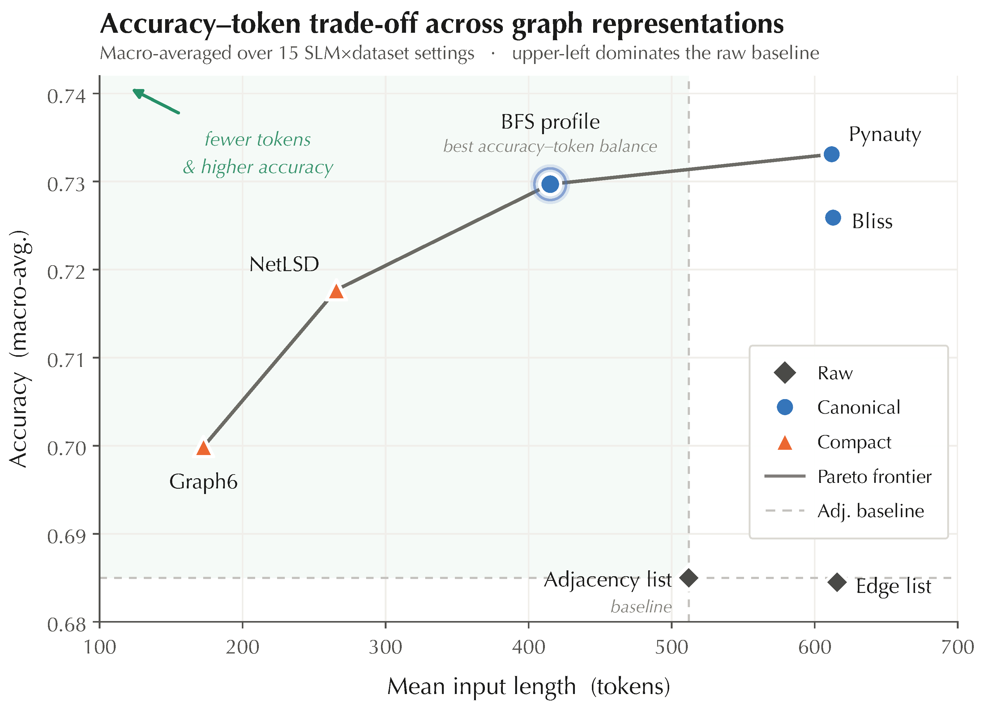

Table 1.
10-fold cross-validation accuracy (mean ± std) across datasets.
| Model | PROTEINS | MUTAG | BZR | PTC_MR | IMDB-BINARY |
| GNN Baselines | |||||
| GCN | 0.7071 ± 0.0466 | 0.6865 ± 0.0961 | 0.8099 ± 0.0419 | 0.5608 ± 0.0517 | 0.6950 ± 0.0453 |
| GIN | 0.7134 ± 0.0372 | 0.7822 ± 0.0795 | 0.7951 ± 0.0194 | 0.5810 ± 0.0508 | 0.7134 ± 0.0372 |
| SAGE | 0.6901 ± 0.0767 | 0.7018 ± 0.0731 | 0.7924 ± 0.0416 | 0.5603 ± 0.0809 | 0.6660 ± 0.0566 |
| GAT | 0.7035 ± 0.0579 | 0.6754 ± 0.0840 | 0.7927 ± 0.0149 | 0.5903 ± 0.0495 | 0.6400 ± 0.0435 |
| Llama-3.2-1B-Instruct | |||||
| Adjacency list | 0.6909 ± 0.0414 | 0.8082 ± 0.0366 | 0.7401 ± 0.0876 | 0.5292 ± 0.0508 | 0.6570 ± 0.0537 |
| Edge list | 0.6881 ± 0.0437 | 0.7848 ± 0.1722 | 0.7624 ± 0.1382 | 0.5236 ± 0.0498 | 0.6530 ± 0.0297 |
| Soft stats MLP | 0.7233 ± 0.0579 | 0.8143 ± 0.0816 | 0.7877 ± 0.0101 | 0.5321 ± 0.0494 | 0.6790 ± 0.0446 |
| Soft GNN | 0.7386 ± 0.0285 | 0.7345 ± 0.1201 | 0.7926 ± 0.0113 | 0.5468 ± 0.0707 | 0.6880 ± 0.0438 |
| Bliss | 0.6945 ± 0.0216 | 0.8246 ± 0.0531 | 0.7703 ± 0.0535 | 0.6098 ± 0.0650 | 0.6860 ± 0.0484 |
| Pynauty | 0.6963 ± 0.0202 | 0.8836 ± 0.0870 | 0.8220 ± 0.0485 | 0.5988 ± 0.0705 | 0.6980 ± 0.0309 |
| BFS profile | 0.7269 ± 0.0442 | 0.8029 ± 0.0871 | 0.8271 ± 0.0709 | 0.5901 ± 0.0443 | 0.6930 ± 0.0461 |
| Graph6 | 0.6945 ± 0.0291 | 0.7611 ± 0.0846 | 0.7779 ± 0.0257 | 0.5355 ± 0.0873 | 0.6840 ± 0.0307 |
| NetLSD | 0.7018 ± 0.0313 | 0.8088 ± 0.0820 | 0.7974 ± 0.0794 | 0.5142 ± 0.0913 | 0.6850 ± 0.0388 |
| Late fusion | 0.7304 ± 0.0326 | 0.8784 ± 0.0527 | 0.8445 ± 0.0469 | 0.6280 ± 0.0709 | 0.7050 ± 0.0512 |
| Qwen2.5-1.5B-Instruct | |||||
| Adjacency list | 0.6775 ± 0.0731 | 0.8085 ± 0.0715 | 0.7684 ± 0.1028 | 0.5469 ± 0.0744 | 0.6320 ± 0.0354 |
| Edge list | 0.7071 ± 0.0523 | 0.8085 ± 0.0484 | 0.7334 ± 0.1078 | 0.5291 ± 0.0908 | 0.6480 ± 0.0340 |
| Soft stats MLP | 0.7081 ± 0.0765 | 0.7713 ± 0.1063 | 0.7877 ± 0.0101 | 0.5289 ± 0.0765 | 0.6560 ± 0.0719 |
| Soft GNN | 0.7216 ± 0.0628 | 0.7459 ± 0.1004 | 0.7902 ± 0.0110 | 0.4999 ± 0.0503 | 0.6690 ± 0.0592 |
| Bliss | 0.7170 ± 0.0354 | 0.8459 ± 0.0546 | 0.7874 ± 0.0531 | 0.5789 ± 0.0717 | 0.6680 ± 0.0821 |
| Pynauty | 0.7071 ± 0.0365 | 0.8781 ± 0.0574 | 0.8001 ± 0.0370 | 0.5697 ± 0.0546 | 0.6990 ± 0.0375 |
| BFS profile | 0.7153 ± 0.0413 | 0.7988 ± 0.1049 | 0.8424 ± 0.0611 | 0.6248 ± 0.0677 | 0.6940 ± 0.0367 |
| Graph6 | 0.6927 ± 0.0389 | 0.8193 ± 0.0855 | 0.7731 ± 0.0557 | 0.5465 ± 0.0938 | 0.6680 ± 0.0223 |
| NetLSD | 0.7287 ± 0.0426 | 0.8406 ± 0.0521 | 0.8248 ± 0.0314 | 0.5585 ± 0.0528 | 0.6770 ± 0.0677 |
| Late fusion | 0.7313 ± 0.0346 | 0.8830 ± 0.0617 | 0.8542 ± 0.0450 | 0.5898 ± 0.0644 | 0.7150 ± 0.0557 |
| SmolLM2-1.7B-Instruct | |||||
| Adjacency list | 0.7162 ± 0.0428 | 0.8354 ± 0.0719 | 0.6912 ± 0.1446 | 0.5520 ± 0.0884 | 0.6210 ± 0.0301 |
| Edge list | 0.6963 ± 0.0322 | 0.8196 ± 0.0706 | 0.7351 ± 0.0226 | 0.5371 ± 0.0933 | 0.6410 ± 0.0579 |
| Soft stats MLP | 0.7376 ± 0.0380 | 0.7652 ± 0.0848 | 0.7877 ± 0.0101 | 0.5640 ± 0.0200 | 0.6890 ± 0.0439 |
| Soft GNN | 0.7368 ± 0.0384 | 0.7240 ± 0.0859 | 0.7877 ± 0.0101 | 0.5729 ± 0.0318 | 0.6960 ± 0.0361 |
| Bliss | 0.6999 ± 0.0371 | 0.8936 ± 0.0471 | 0.8246 ± 0.0464 | 0.6165 ± 0.0584 | 0.6710 ± 0.0421 |
| Pynauty | 0.6945 ± 0.0572 | 0.8462 ± 0.1085 | 0.8246 ± 0.0462 | 0.5989 ± 0.1132 | 0.6800 ± 0.0397 |
| BFS profile | 0.7269 ± 0.0274 | 0.8178 ± 0.0729 | 0.8224 ± 0.0457 | 0.5787 ± 0.0725 | 0.6850 ± 0.0258 |
| Graph6 | 0.7062 ± 0.0455 | 0.8456 ± 0.0373 | 0.7460 ± 0.0845 | 0.5607 ± 0.0809 | 0.6880 ± 0.0325 |
| NetLSD | 0.6990 ± 0.0281 | 0.8354 ± 0.0592 | 0.8023 ± 0.0375 | 0.5670 ± 0.0713 | 0.7250 ± 0.0377 |
| Late fusion | 0.7386 ± 0.0359 | 0.8833 ± 0.0454 | 0.8518 ± 0.0400 | 0.6365 ± 0.0843 | 0.6980 ± 0.0498 |
Table 2.
Aggregate accuracy over all five datasets. Lower average rank is better.
| Method | Llama | Qwen | Smol | Overall | vs Adj. | Avg. rank |
| Adjacency list | 0.6851 | 0.6867 | 0.6832 | 0.6850 | – | 8.20 |
| Edge list | 0.6824 | 0.6852 | 0.6858 | 0.6845 | -0.0005 | 8.73 |
| Soft stats MLP | 0.7073 | 0.6904 | 0.7087 | 0.7021 | +0.0172 | 6.37 |
| Soft GNN | 0.7001 | 0.6853 | 0.7035 | 0.6963 | +0.0113 | 5.70 |
| Bliss | 0.7170 | 0.7194 | 0.7411 | 0.7259 | +0.0409 | 4.63 |
| Pynauty | 0.7397 | 0.7308 | 0.7288 | 0.7331 | +0.0482 | 4.00 |
| BFS profile | 0.7280 | 0.7351 | 0.7262 | 0.7297 | +0.0448 | 4.27 |
| Graph6 | 0.6906 | 0.6999 | 0.7093 | 0.6999 | +0.0150 | 6.87 |
| NetLSD | 0.7014 | 0.7259 | 0.7257 | 0.7177 | +0.0327 | 4.90 |
| Late fusion | 0.7573 | 0.7547 | 0.7616 | 0.7579 | +0.0729 | 1.33 |
Table 3.
Accuracy–token trade-off across all datasets and SLM backbones. Accuracy is macro-averaged over 15 model–dataset settings. Token length is the mean input length; positive token reduction means shorter than the adjacency-list representation.
Table 3.
Accuracy–token trade-off across all datasets and SLM backbones. Accuracy is macro-averaged over 15 model–dataset settings. Token length is the mean input length; positive token reduction means shorter than the adjacency-list representation.
| Representation | Type | Accuracy | vs Adj. | Mean tokens | Token reduction |
| Adjacency list | Raw | 0.6850 | – | 511.9 | – |
| Edge list | Raw | 0.6845 | -0.0005 | 615.7 | -20.3% |
| Bliss | Canonical | 0.7259 | +0.0409 | 612.9 | -19.7% |
| Pynauty | Canonical | 0.7331 | +0.0482 | 611.9 | -19.5% |
| BFS profile | Canonical | 0.7297 | +0.0448 | 415.1 | +18.9% |
| Graph6 | Compact | 0.6999 | +0.0150 | 172.7 | +66.3% |
| NetLSD | Compact | 0.7177 | +0.0327 | 265.6 | +48.1% |
Disclaimer/Publisher’s Note: The statements, opinions and data contained in all publications are solely those of the individual author(s) and contributor(s) and not of MDPI and/or the editor(s). MDPI and/or the editor(s) disclaim responsibility for any injury to people or property resulting from any ideas, methods, instructions or products referred to in the content. |
© 2026 by the authors. Licensee MDPI, Basel, Switzerland. This article is an open access article distributed under the terms and conditions of the Creative Commons Attribution (CC BY) license (http://creativecommons.org/licenses/by/4.0/).
Copyright: This open access article is published under a Creative Commons CC BY 4.0 license, which permit the free download, distribution, and reuse, provided that the author and preprint are cited in any reuse.