

Submitted:
31 July 2026
Posted:
31 July 2026
You are already at the latest version
Abstract
Land subsidence is a widespread geological hazard in urban areas, yet accurate prediction remains challenging due to the complex, non-linear spatio-temporal dynamics governing subsurface deformation. In this work, the PEGNet (Peridynamics-Emergent-GAT-GRU Network) method integrates Graph Attention Networks (GAT) with Gated Recurrent Units (GRU) under a three-level embedding strategy to predict land subsidence at monitoring points. Peridynamics gradient and emergent velocity features are fused with multi-source data at the feature level; multi-head graph attention captures spatial dependencies among monitoring points at the structure level; and a Peridynamics-based loss regularizer penalizes unrealistic spatial gradients while an attention entropy regularizer encourages focused attention patterns at the constraint level. Evaluated in Tongzhou District, Beijing over 60 months, the model achieves an RMSE of 5.16 mm, outperforming the GAT-GRU baseline by 25.1% and reducing RMSE by 51.7% relative to GCN-LSTM. Comprehensive ablation studies and baseline comparisons validate each component, showing that the dual-constraint framework effectively suppresses large-magnitude outliers. This work demonstrates that coupling macro-micro priors with spatio-temporal deep learning provides an effective paradigm for integrating physical and geoscience principles into data-driven subsidence prediction.
Keywords:
land subsidence prediction
; spatio-temporal neural network
; Graph Attention Networks
; Peridynamics
; emergent features
; deep learning
; PEGNet
1. Introduction
Land subsidence is a geological hazard of growing global concern, characterized by increasing complexity, risk, and uncertainty [1,2]. The North China Plain, due to long-term intensive groundwater extraction, has developed the world's largest groundwater depression cone and the most extensive land subsidence area [3,4]. In Beijing, groundwater over-extraction has become the primary driver of land subsidence occurrence and development [3]. In recent years, the South-to-North Water Diversion Project has altered the regional water balance, leading to groundwater recovery in parts of Beijing and a deceleration of subsidence in some areas [5,6], adding new complexity to the spatio-temporal evolution of land subsidence. Precipitation is a key driver of groundwater recharge and a fundamental parameter in subsidence studies [7]. Climate change, through altered water cycles and more frequent extreme precipitation events, has introduced additional uncertainty into the long-term evolution of land subsidence. As Tongzhou has been designated as Beijing's deputy city center, understanding and accurately predicting subsidence patterns in this area is critical for infrastructure safety and sustainable urban development [8].
Physics-driven mechanistic models have long dominated subsidence simulation. These geomechanical models, typically implemented via numerical methods, offer interpretability and physical consistency for long-term scenario projections through rigorous theoretical formulations. However, these models often require extensive calibration data and face challenges in parameterizing heterogeneous aquifer systems [9]. In the Beijing Plain, where hydrogeological conditions are highly heterogeneous with multi-layered aquifer configurations, oversimplified assumptions and difficulties in parameter calibration lead to notable discrepancies between simulated and observed deformations [10,11]. Conventional statistical approaches, including regression models and Grey-Markov chains, are typically limited to simple deformation trends and cannot capture complex spatial interactions among monitoring points [12,13]. Similarly, more advanced machine learning and data-driven methods remain at a point-scale prediction level without modeling the spatial dependencies of the monitoring network [14,15,16].
Deep learning has substantially advanced spatio-temporal prediction in recent years. Recurrent Neural Networks (RNNs), including Long Short-Term Memory (LSTM) networks and Gated Recurrent Units (GRU), achieve strong performance in sequential modeling [17,18], while Graph Neural Networks (GNNs), particularly Graph Attention Networks (GATs) [19], naturally process irregular spatial structures [20]. Hybrid GNN-RNN architectures have demonstrated state-of-the-art results across diverse Earth science applications [21,22,23,24]. For subsidence prediction specifically, attention-based LSTM models have shown promising results [25,26,27], and Transformers have been explored for long-range temporal dependencies [28]. In the eastern Beijing Plain, Cao et al. [26] proposed an AM-LSTM (Attention Mechanism-LSTM) with improved performance. However, these approaches remain purely data-driven: they lack explicit integration with hydrogeomechanical principles and do not model spatial interactions among monitoring points, limiting their capacity to capture the physical mechanisms driving subsidence and producing potentially implausible predictions beyond the training distribution [29,30,31].
Physics-Informed Neural Networks (PINNs) represent a significant step toward bridging this gap by embedding physical laws as soft constraints within the loss function [32,33]. However, PINNs require explicit partial differential equation (PDE) formulations, which are often unavailable for heterogeneous aquifer systems with complex boundary conditions and sparse monitoring data [34]. Peridynamics (PD) offers an alternative theoretical framework that describes deformation through non-local integral equations without requiring PDEs [35,36]. The PD gradient, which quantifies local deformation intensity by measuring relative displacements between neighboring material points, can be computed directly from monitoring data using the existing graph structure, making it naturally compatible with GNN-based architectures. Recent studies have demonstrated the applicability of peridynamics to regional subsidence modeling in the Beijing Plain [37,38], establishing a foundation for integrating continuum mechanics into spatio-temporal deep learning. The coupling of physical mechanisms with data-driven approaches represents a transformative paradigm in the geosciences, yet most existing hybrid methods remain at a shallow integration level, incorporating physics only as loss penalties rather than embedding mechanistic knowledge throughout the entire modeling pipeline, from feature engineering to model architecture and constraint design [31,39].
Emergent features, grounded in complex system theory, capture macroscopic behavioral patterns that arise from collective microscale interactions rather than from explicit physical first principles [40]. The emergent velocity of subsidence reflects the self-organizing dynamics of the deformation field and provides a data-driven complement to physics-based gradient constraints. Beyond serving as an input feature, this emergent information also informs a constraint-level attention entropy regularizer that encourages focused and interpretable attention patterns. Geographic principles further underpin the modeling framework: Tobler's first law of geography, which states that near points are more related than distant points [41], provides the theoretical basis for graph construction based on spatial proximity, while the principle of spatial heterogeneity motivates the use of adaptive attention mechanisms across the monitoring network [20].
This paper proposes PEGNet (Peridynamics-Emergent-GAT-GRU Network), a spatio-temporal deep learning framework that integrates Graph Attention Networks with Gated Recurrent Units under a three-level prior embedding strategy. The core innovation lies in coupling Peridynamics gradient constraints and emergent velocity features within a unified architecture:
- At the feature level, PD gradient features and emergent velocity features are fused with multi-source inputs (subsidence, groundwater level, groundwater storage anomaly and precipitation) as additional input channels, providing the GAT encoder with explicit deformation gradient and subsidence rate information;
- At the structure level, multi-head graph attention adaptively captures spatial dependencies among monitoring points in Tongzhou District, Beijing, with the graph constructed via KD-tree search based on geographic proximity;
- At the constraint level, a PD-based loss regularizer penalizes physically implausible spatial gradients in the predictions while an attention entropy regularizer encourages focused and interpretable attention patterns.
The model is evaluated on 60 months (from January 2018 to December 2022) of PS-InSAR observations and multi-source hydrogeological data in Tongzhou District, Beijing. Extensive ablation studies and comprehensive baseline comparisons are conducted to validate the contribution of each component.
2. Materials and Methods
2.1. Study Area
Tongzhou District, eastern Beijing (116.2E–116.8E, 39.7N–40.0N), covers approximately 907 km² and serves as Beijing's deputy city center since 2015. The district lies on the alluvial plain, underlain by a thick Quaternary aquifer system comprising multiple confined aquifers interbedded with compressible clay layers. The study area is affected by the regional fault system of the North China Plain (Figure 1 (a)), exhibiting significant spatial heterogeneity in stratum thickness and sedimentary structure. The vertical profile consists of extensive Quaternary loose sediments, dominated by clay, silty clay, and sandy interbedded strata, forming a Quaternary aquifer system highly susceptible to consolidation deformation under groundwater level decline. Long-term groundwater abstraction and rapid urban construction have jointly altered pore water pressure and effective stress in shallow and middle aquifers, driving continuous and uneven land subsidence [7]. These characteristics make Tongzhou District a representative area for investigating the spatiotemporal evolution and intelligent prediction of land subsidence.
2.2. Dataset Description
A total of 13,505 persistent scatterers (PS) were derived from 73 scenes of Sentinel-1A imagery (from May 2017 to May 2023) using PS-InSAR processing [42], with line of sight (LOS) deformation converted to vertical displacement and validated against leveling survey data (maximum annual rate error < 10 mm/yr). For this study, 60 consecutive months (from January 2018 to December 2022) of vertical displacement time series were extracted for each scatterer, together with three auxiliary raster datasets covering hydrogeological and meteorological drivers: (i) monthly vertical subsidence (incremental deformation and cumulative deformation); (ii) shallow groundwater level at 1 km monthly resolution [43] and groundwater storage anomaly (GWSA) at 0.5° resolution [44]; and (iii) precipitation at 1 km monthly resolution [45]. All auxiliary raster data were assigned to each PS scatterer by directly sampling the corresponding grid cell value at the scatterer's geographic coordinate, without spatial interpolation. Consequently, all input features share a uniform monthly temporal resolution and PS-point spatial resolution, as visualized in Figure 1b-e.
The study period (2018–2022) covers a complete water cycle phase in the Beijing Plain, during which the South-to-North Water Diversion Project has gradually altered regional groundwater storage dynamics [6,10]. The 60-month window captures both the seasonal fluctuations and the interannual trend of subsidence, providing sufficient temporal depth for training spatiotemporal models with a 24-month input horizon. Each variable was independently normalized to [0,1] using MinMaxScaler. A sliding window (24-month input, 6-month prediction, stride = 1) yielded 31 samples, split chronologically into 19 training, 6 validation, and 6 test sets.
2.3. PEGNet Architecture
Figure 2 illustrates the overall framework of PEGNet. Two complementary constraints, a physics-informed Peridynamics gradient constraint and a data-driven emergent velocity feature, are embedded into a four-stage spatio-temporal architecture: graph construction and feature fusion, GAT-based spatial encoding, GRU-based temporal modeling, and dual-constraint optimization. The main workflow proceeds as follows:
- Graph construction and feature fusion. A spatial graph is built from PS scatterer coordinates using KD-tree search with a distance-based pruning threshold. Multi-source input variables are augmented with Peridynamics gradient features and emergent velocity features to form a fused representation that encodes both local deformation mechanics and macroscopic subsidence trends.
- GAT Spatial encoding. At each time step, a multi-head Graph Attention Network (GAT) adaptively aggregates information from neighboring scatterers, learning spatially varying attention weights that reflect the heterogeneity of subsidence patterns across the study area.
- GRU Temporal modeling. The spatially encoded features across all input time steps are processed by a Gated Recurrent Unit (GRU), which captures the long-term temporal evolution of subsidence through its gating mechanism.
- Prediction and dual-constraint regularization. The final hidden state of the GRU is mapped to the prediction output through a linear layer. During training, two regularizers are jointly optimized: a Peridynamics-based loss that penalizes unrealistic spatial gradients in the predicted deformation field, and an attention entropy regularizer that encourages focused attention patterns.
The specific methodological components are described in detail in the following subsections.
2.3.1. Graph Construction and Feature Fusion
The spatial graph serves as the structural backbone for both constraints in PEGNet. The PD gradient requires graph edges to compute local deformation gradients between neighboring scatterers, while the emergent velocity, though computed per node independently, provides a macroscopic context that complements the local interactions captured by the graph. Accordingly, an undirected graph is first constructed from the geographic coordinates of all PS scatterers using KD-tree search (k = 20, 1 km threshold), yielding approximately 305,000 edges. Edge weights represent the Euclidean distance between connected nodes.
The framework adopts a channel-level concatenation strategy to fuse three categories of features. The original input feature tensor contains all variables across T time steps. Two enhancement features are computed and concatenated along the channel dimension:
Peridynamics gradient features. Peridynamics (PD) is a non-local continuum theory that describes deformation through spatial integral equations rather than partial differential equations [35,36]. In the ordinary state-based PD formulation, the equation of motion for a material point x at time t is:
where is the material density, is the acceleration, is the horizon (neighborhood) of x defined by radius δ, T is the force state vector, and b is the body force density.
In the context of subsidence monitoring, we adopt a simplified, data-driven form of the PD gradient that measures local deformation intensity from the existing scatterer graph:
where is the monthly subsidence at node i, is the edge weight, is the node degree, and N(i) is the neighbor set. The gradient is computed independently for each time step, producing a per-node per-step feature .
Emergent velocity features. The emergent velocity captures the macroscopic subsidence trend over the input window, motivated by the concept that coherent macroscopic patterns can arise from coupled interactions at smaller scales. Rather than classifying scatterers into discrete subsidence rate categories, which would impose arbitrary thresholds and discard information about gradual spatial transitions [4,15], we retain velocity as a continuous feature. The average subsidence velocity for scatterer i is:
where and are the cumulative deformation at the first- and last-time steps. Unlike monthly subsidence and cumulative deformation, which capture short-term fluctuations and total accumulated deformation respectively, the emergent velocity describes the directional rate of change over the entire window. These three metrics are complementary: monthly subsidence provides fine-grained dynamics, cumulative deformation tracks long-term accumulation, and velocity encodes the underlying temporal trend. The scalar is expanded to match the temporal dimension, forming .
The final fused feature tensor is:
where ⊕ denotes channel-wise concatenation. The fused representation thus contains three complementary information levels: raw monitoring measurements, local deformation gradients derived from continuum mechanics, and a macroscopic trend descriptor of subsidence evolution. This multi-scale feature tensor is then passed to the GAT encoder for spatial feature extraction.
2.3.2. GAT Spatial Encoding
The GAT module serves as the core spatial component of the PEGNet framework, leveraging a self-attention mechanism to learn edge weights dynamically from the fused multi-scale features [19]. Unlike GCNs [20] that assign fixed and identical weights to all neighboring nodes, GAT adaptively highlights the influence of nodes with similar subsidence characteristics or deformation traits, while downweighting irrelevant or noisy connections.
For each node i and its neighbor j at a given time step, the attention coefficient is computed as:
where W is a shared linear transformation matrix, a is the attention vector, denotes feature concatenation, and N(i) is the neighbor set of node i. The softmax function normalizes the raw attention scores across all neighbors, ensuring the sum of attention weights for each node equals 1. Multi-head attention is used to stabilize the learning process.
This attention-driven design is well suited to the inherent spatial heterogeneity of land subsidence: scatterers under similar hydrogeological conditions or exhibiting comparable deformation patterns receive higher mutual attention, enabling the model to capture physically meaningful spatial correlations while suppressing noise. The resulting spatially encoded features across all time steps are then passed to the GRU module for temporal modeling.
2.3.3. GRU Temporal Encoding
The GRU module receives the spatially encoded feature sequence from the GAT module and models the temporal dynamics of land subsidence [18]. As a simplified variant of LSTM, the GRU retains the gating mechanism to address gradient vanishing in long-sequence modeling while reducing computational complexity, making it suitable for the slow-varying characteristics of hydrogeological processes.
For a given timestep t, the input is the spatial feature vector at that timestep, and is the previous hidden state. The core operations are:
where and are the update and reset gates, is the candidate hidden state, W and U are weight matrices, b are bias vectors, σ is the sigmoid function, and denotes element-wise multiplication [18]. Through this gating mechanism, the GRU captures the long-term temporal evolution of subsidence while preserving the spatiotemporally fused features derived from both the PD gradient and emergent velocity constraints. The final hidden state serves as the spatio-temporal feature representation for each scatterer, which is then passed to the output layer for prediction.
2.3.4. Dual-Constraint Regularization and Loss Function
The total loss function of PEGNet combines data fidelity with two physics-informed regularizers:
where is the data fitting loss between predictions and observations; =mean(g²) is the Peridynamics gradient loss that penalizes unrealistic spatial gradients in the predicted deformation field, and g is the PD gradient magnitude at each node; =mean(H(α)) is the emergent pattern regularization term computed as the average attention entropy across all GAT heads and edges, and α denotes the attention weight distribution across neighbors. and are the weighting coefficients. Minimizing this entropy encourages the attention mechanism to focus on a sparse subset of informative neighbors, producing more interpretable and selective spatial weights.
The weighting coefficients and control the contribution of each constraint. Through grid search, the optimal values were determined as = 5.0 and = 1.0 for single-constraint ablation variants, and = 0.5 and = 0.2 for the combined PEGNet model. The reduced weights in the combined configuration reflect a partial trade-off between the smoothness prior (PD) and the sparsity prior (entropy), as both regularizers act on the spatial distribution of predictions. Gradient clipping with a maximum norm of 1.0 is applied during training to prevent gradient explosion from the GAT and PD layers.
2.4. Experimental Setup
All models were implemented in PyTorch 2.6.0 with PyTorch Geometric 2.8.0 and trained on an NVIDIA RTX 4060 Ti GPU (8 GB VRAM). The Adam optimizer was used with a learning rate of 1e-3, a batch size of 1, and gradient clipping at a norm of 1.0. Training was run for a maximum of 50 epochs with early stopping (patience = 5), and all experiments used a fixed random seed of 42.
Four evaluation metrics were adopted. Let and denote the observed and predicted cumulative deformation for sample , respectively, and the mean of the observations. The Root Mean Square Error (RMSE) and Mean Absolute Error (MAE) quantify the absolute deviation between predictions and observations:
The Nash-Sutcliffe Efficiency (NSE) [46] measures the proportion of variance explained by the model relative to the observed mean:
The Kling-Gupta Efficiency (KGE) [47] decomposes model performance into correlation, variability, and bias components:
where r is the Pearson correlation coefficient, is the variability ratio, and is the bias ratio. All metrics were computed on the test set (windows 25–30, corresponding to February 2022–December 2022).
3. Results
3.1. Model Performance Comparison
The overall performance of all six models is evaluated from three perspectives. Figure 3 compares the models on the test set, ordered by architectural complexity: three baselines establish the encoder choices (GCN-LSTM, GCN-GRU, GAT-GRU), two ablation variants isolate the contribution of each constraint (PD-GAT-GRU, EF-GAT-GRU), and the full PEGNet integrates both. This hierarchical design enables systematic assessment of temporal encoding, spatial encoding, and physics-informed constraints within a unified framework.
Among the three baseline models, the choices of temporal and spatial encoders both have a substantial impact. GRU-based models consistently outperform LSTM-based ones: GCN-GRU (RMSE 7.63 mm) achieves a 29% reduction over GCN-LSTM (10.69 mm), confirming that the GRU gating mechanism is better suited to the slow-varying dynamics of land subsidence. Replacing GCN with GAT yields a further improvement: GAT-GRU (RMSE 6.89 mm) outperforms GCN-GRU (7.63 mm), demonstrating that adaptive attention weights capture spatial heterogeneity across PS scatterers more effectively than fixed spectral convolution.
The ablation study further validates the contribution of each proposed component. Adding the PD gradient alone (PD-GAT-GRU) reduces RMSE to 6.34 mm and raises KGE to 0.8951; adding the emergent velocity alone (EF-GAT-GRU) achieves RMSE of 6.09 mm and KGE of 0.9015. Both physics-informed constraints provide complementary gains, and when integrated in the full PEGNet framework, the model achieves the best overall performance (RMSE 5.16 mm, MAE 3.80 mm, NSE 0.9850, and KGE 0.9191) representing a 51.7% RMSE reduction relative to GCN-LSTM.
Figure 4 presents the error distribution of all six models from two complementary perspectives. The CDF panel (Figure 4a) shows that PEGNet consistently dominates across the entire error range: 74% of its predictions have absolute errors below 5 mm and 94% below 10 mm, compared to 59% and 86% for GAT-GRU and 58% and 83% for GCN-GRU. The 90th percentile error of PEGNet is 8.5 mm, substantially lower than those of GAT-GRU (11.4 mm) and GCN-GRU (12.6 mm). The gap between models widens at the upper tail, confirming that the dual-constraint framework is particularly effective at suppressing large-magnitude outliers.
The error density panel (Figure 4b) further reveals the directional bias of each model's predictions using raw errors (predicted minus observed). The density peak of PEGNet is centered closest to zero and exhibits the narrowest spread among all models, confirming that it produces the least biased predictions. In contrast, GCN-LSTM and, to a lesser extent, GAT-GRU show density peaks shifted toward positive values, indicating systematic overestimation of cumulative deformation. The ablation variants (PD-GAT-GRU and EF-GAT-GRU) occupy intermediate positions, consistent with their RMSE rankings. The combination of CDF and density plots provides a complete picture of both error magnitude and bias direction.
Figure 5 presents the scatter density of predicted versus observed cumulative deformation for all six models. The regression slope improves progressively from 0.849 (GCN-LSTM, Figure 5a) to 0.901 (GCN-GRU, Figure 5b), 0.916 (GAT-GRU, Figure 5c), 0.924 (PD-GAT-GRU, Figure 5d), 0.929 (EF-GAT-GRU, Figure 5e), and 0.936 (PEGNet, Figure 5f), confirming that each enhancement, including GRU over LSTM, GAT over GCN, and the two physics-informed constraints, reduces systematic bias. PEGNet achieves the slope closest to unity, demonstrating that the dual-constraint framework effectively guides predictions toward the observed deformation field.
3.2. Spatio-Temporal Prediction Results
The test set comprises six temporal windows (windows 25–30), covering February 2022 to December 2022. Within each test window, the model generates six consecutive monthly forecasts, referred to as Step 1 through Step 6. Since the six test windows start at different time points, all results reported in this section are averaged over the six test windows to reflect the model's average prediction performance rather than its performance on a single window.
Figure 6 compares the cumulative deformation predictions of all six models against the observed data at the first prediction step (February 2022). All models produce spatial patterns consistent with the observed deformation field, with mild local underestimation in the subsidence funnel across most models. PEGNet (Figure 6g) achieves the closest agreement with the observed values (Figure 6a), while GCN-LSTM (Figure 6b) shows slightly larger deviations. At the last prediction step (December 2022, Figure A1), GCN-LSTM and GCN-GRU exhibit substantial underestimation across the study area, while the four GAT-based models produce predictions that remain relatively consistent with the observations, although underestimation in the funnel core persists to some extent.
To further examine the prediction performance at the point scale, Figure 7 shows the full time series at three representative PS scatterers classified by their annual subsidence rate: severe (≥30 mm/yr), moderate (10-30 mm/yr), and slight (≤10 mm/yr), using the first test window (from February 2022 to July 2022). The black line denotes the observed values. Across all three subsidence regimes, PEGNet produces predictions closest to the observed values, confirming the effectiveness of the dual-constraint framework. The GAT-based models (GAT-GRU, PD-GAT-GRU, EF-GAT-GRU) also perform well, with predictions closely tracking the observations and largely overlapping with PEGNet. In the severe (Figure 7a) and moderate (Figure 7b) subsidence cases, GCN-LSTM and GCN-GRU exhibit a clear negative bias, substantially underestimating the cumulative deformation magnitude, consistent with their lower accuracy reported in Section 3.1. At the slight subsidence point (Figure 7c), where the annual rate is below 10 mm/yr, all models converge to a similar flat trend, reflecting the inherently low deformation magnitude at this location.
The corresponding predictions averaged across all six test windows are shown in Figure A2. The averaging process smooths individual trajectories, making the predictions less responsive to month-to-month variations while preserving the same relative model ranking: PEGNet maintains the closest agreement with the observations, GAT-based models form a tight cluster, and GCN-based models exhibit systematic underestimation in high-deformation areas.
3.3. Spatio-Temporal Error Analysis
To systematically evaluate the prediction errors of all models, this section provides a multi-perspective analysis covering spatial error distribution, lead-time dependence, and combined spatio-temporal error structure. The per-point RMSE is computed for each scatterer over the six prediction steps and then averaged across all scatterers to obtain the reported mean value.
Figure 8 maps the spatial distribution of per-point RMSE across all six model configurations. GCN-LSTM (Figure 8a) exhibits a mean per-point RMSE of 8.70 mm, with 15% of scatterers exceeding 15 mm, concentrated in the northwestern subsidence funnel. GCN-GRU (Figure 8b) reduces the mean to 6.33 mm and the high-error proportion to 5%. GAT-GRU (Figure 8c) further improves the mean to 5.86 mm. Adding the PD gradient constraint (PD-GAT-GRU, Figure 8d) and the emergent velocity feature (EF-GAT-GRU, Figure 8e) yields incremental improvements to 5.43 mm and 5.23 mm, respectively. PEGNet (Figure 8f) achieves the lowest mean RMSE of 4.45 mm, with virtually no scatterers exceeding 15 mm. The proportion of scatterers with RMSE below 5 mm increases progressively from 37% (GCN-LSTM) to 49% (GCN-GRU), 51% (GAT-GRU), 55% (PD-GAT-GRU), 57% (EF-GAT-GRU), and 66% (PEGNet). The progressive reduction in high-error outliers confirms that each enhancement contributes to suppressing prediction errors, with the dual-constraint framework in PEGNet being most effective in regions with steep subsidence gradients.
Figure 9 examines how prediction accuracy evolves with lead time by presenting the per-step RMSE of all six models across Step 1 to Step 6, with numerical values summarized in Table A3. PEGNet achieves the lowest RMSE at four of the six steps (Steps 1, 2, 4, and 5) and obtains the best overall RMSE of 5.16 mm. At Step 3, PD-GAT-GRU achieves the lowest value (4.69 mm), and at Step 6, EF-GAT-GRU performs best (4.22 mm). The performance degradation from Step 1 to Step 6 is most pronounced for GCN-LSTM, whose RMSE increases from 9.93 mm to 12.09 mm, and least for PEGNet, which exhibits a relatively flat error trajectory. This indicates that the dual physics-informed constraints not only reduce overall error but also stabilize predictions over longer lead times.
Figure 10 maps the per-point residuals (predicted minus observed) averaged over all six test windows at the first prediction step (from February 2022 to July 2022). PEGNet (Figure 10f) displays the most spatially uniform residual distribution with a mean bias close to zero, consistent with its lowest RMSE at Step 1 (Figure 9). At the third and sixth steps (see per-step RMSE in Figure 9), however, PEGNet's residual magnitude exceeds that of PD-GAT-GRU and EF-GAT-GRU individually, indicating that the dual constraints may partially interact under longer lead times. Despite this, the GAT-GRU backbone remains robust: even at the last prediction step averaged over the six test windows (from July 2022 to December 2022, Figure A4), GAT-GRU, PD-GAT-GRU, and EF-GAT-GRU maintain competitive performance with RMSE values well below GCN-based models. The fact that PD-GAT-GRU and EF-GAT-GRU outperform their combination in PEGNet at later steps suggests that the weighting or interaction between the two constraints has room for further optimization through hyperparameter tuning rather than reflecting a fundamental limitation of the framework.
3.4. Hyperparameter Sensitivity Analysis
To investigate the interaction between the two regularization terms, a grid search was conducted over the weighting coefficients and . The grid evaluated values of {0, 0.2, 0.5, 1.0, 2.0, 5.0, 10.0} for single-constraint variants and selected combinations for the joint PEGNet model. The RMSE from the grid search is reported in Table 1.
When applied individually, the optimal weights are = 5.0 for the PD gradient loss and = 1.0 for the emergent entropy regularizer. However, directly combining these individually optimal weights produces a joint RMSE of 6.26 mm, which is worse than the GAT-GRU baseline (5.13 mm on the validation set). This indicates a partial conflict between the two regularization objectives. The PD loss encourages spatial smoothness by penalizing large local gradients, while entropy minimization encourages the attention mechanism to focus on a sparse subset of neighbors, which can lead to less spatially smooth attention patterns.
The best joint configuration requires substantially reduced weights ( = 0.5, = 0.2), achieving a validation RMSE of 4.16 mm. The final PEGNet model, re-trained with these optimal weights, achieves an RMSE of 5.16 mm, confirming that the two regularizers capture complementary aspects of physically plausible deformation despite their partial conflict.
4. Discussion
4.1. Spatio-Temporal Architecture for Land Subsidence
PEGNet is designed around two characteristics of land subsidence monitoring data: irregular spatial distribution and slow temporal evolution. The PS scatterers from InSAR processing are irregularly distributed, with dense urban coverage and sparse peripheral zones. Unlike grid-based architectures, the GAT module operates directly on the graph structure defined by scatterer coordinates, capturing local deformation gradients near fault-bounded geological boundaries without requiring interpolation or grid resampling. The multi-head attention mechanism learns spatially varying correlation patterns, for example weighting scatterers within the same hydrogeological unit more heavily while reducing influence across structural boundaries.
Land subsidence evolves over months to years through gradual processes including aquifer consolidation and seasonal groundwater fluctuations. Although the model predictions appear smoother than the observed time series due to the averaging over six test windows (Figure 7), the GRU module's two-gate architecture is well suited to this slow-varying regime and reduces overfitting risk on the limited 60-month window. The 29% RMSE reduction from GCN-LSTM to GCN-GRU confirms that GRU-based temporal encoding is more effective than LSTM for this dataset.
The decoupled design, in which GAT adaptively weights neighbor contributions through learned attention coefficients at each time step before GRU temporal modeling, is validated: replacing GCN with GAT improves RMSE by 9.7%, while replacing LSTM with GRU improves it by 29%. The attention mechanism captures spatial heterogeneity more flexibly than the fixed normalization in GCN, which is critical for a study area where deformation patterns vary substantially across the northwestern subsidence funnel and the southeastern stable zone.
Compared with existing subsidence prediction approaches, PEGNet provides a structured framework that jointly models spatial dependence, temporal evolution, and physical consistency within a unified architecture. Earlier studies on the Beijing Plain, such as the Grey-Markov model [7] and machine learning approaches incorporating multiple driving factors [15], focused primarily on point-scale prediction without modeling spatial interactions among monitoring points. More recently, attention-based LSTM models [26] achieved improved performance for subsidence simulation in the eastern Beijing Plain by capturing temporal dependencies more effectively, yet these approaches did not incorporate spatial graph structures or physics-informed constraints. PEGNet extends these lines of work by introducing a decoupled spatio-temporal architecture augmented with Peridynamics gradient constraints and emergent feature regularizers, offering a more comprehensive framework that addresses both the spatial heterogeneity and the temporal dynamics of land subsidence.
4.2. Effectiveness of PD Gradient and Emergent Velocity Constraints
The PD gradient operates through two mechanisms: feature augmentation and loss regularization. Feature augmentation provides the GAT with explicit local gradient information at each input time step, while the PD loss penalizes unrealistic spatial gradients in predictions. Both mechanisms use the existing graph structure without additional trainable parameters. The 8.0% RMSE improvement from GAT-GRU (6.89 mm) to PD-GAT-GRU (6.34 mm) demonstrates that even this simple physical prior provides meaningful regularization.
The emergent velocity captures the average subsidence rate over the 24-month input window. Its standalone contribution (11.6% improvement, from 6.89 mm to 6.09 mm) indicates that encoding trend information reduces the modeling burden on the GRU, allowing it to focus on deviations from the linear trend rather than learning the rate of change from raw sequential data. The velocity is retained as a continuous variable to preserve information about gradual spatial transitions between deformation zones.
PEGNet embeds geoscientific constraints at the feature, structure, and optimization levels without adding parameters to the base architecture. Transformer-based models that rely solely on self-attention can produce physically unreasonable predictions in complex geological settings, whereas PEGNet imposes basic geomechanical principles through its multi-level design.
The interaction between the two regularizers warrants attention. As shown by the grid search results (Table 1), the PD loss encourages spatial smoothness while the entropy minimization promotes focused attention patterns. When combined at their individually optimal weights, these objectives conflict and degrade performance. The best joint configuration requires reduced weights that balance smoothness against sparsity. Despite this tension, the combined model outperforms both single-constraint variants, confirming that the two regularizers capture complementary aspects of physically plausible deformation.
4.3. Limitations of the Current Framework
Despite the promising results, several limitations should be acknowledged.
Model-wise, the GAT's spatial feature capture is constrained by the fixed graph topology and neighborhood size, potentially overlooking large-scale aquifer connectivity and long-distance subsidence transmission pathways. The GRU module's ability to fit extreme events, such as heavy precipitation-induced shallow groundwater level recovery, is limited by its reliance on historical data patterns rather than explicit extreme-event response mechanisms.
Data-wise, the model uses shallow groundwater level as a primary hydrogeological input, while the Beijing aquifer system consists of multiple confined layers with distinct piezometric heads. This limitation is partially mitigated by the inclusion of GWSA from satellite gravimetry, which integrates total water storage changes across the entire aquifer system, including deeper confined layers. The current framework does not incorporate anthropogenic factors such as underground construction activities or land use changes, which can significantly influence local subsidence dynamics. Furthermore, the dataset lacks detailed hydrogeological parameters (e.g., layer-specific permeability and storage coefficients), which would require dedicated field campaigns to obtain.
Application-wise, PEGNet is calibrated specifically for the Beijing Plain, and its generalization to other geological settings, such as loess plateaus or karst regions, remains untested. The model also does not account for feedback effects of subsidence on aquifer storage capacity, limiting its utility for long-term coupled water-resources and subsidence management.
To address these limitations, future efforts could focus on incorporating dynamic graph learning to capture evolving aquifer connectivity, integrating higher-resolution InSAR and LiDAR data, and validating the model across different geological settings. Extending the framework to a coupled groundwater-subsidence-aquifer storage model would further enhance its utility for integrated water resource management.
5. Conclusions
This paper presented PEGNet, a spatio-temporal deep learning framework integrating Graph Attention Networks, Gated Recurrent Units, Peridynamics gradient constraints, and emergent velocity features for land subsidence prediction. The model was evaluated on 13,505 persistent scatterers in Tongzhou District, Beijing over a 60-month period (January 2018 to December 2022).
Each proposed enhancement contributes positively to prediction accuracy. The PD gradient constraint reduces RMSE from 6.89 mm (GAT-GRU baseline) to 6.34 mm; the emergent velocity features achieve 6.09 mm; and their combination in PEGNet yields the best overall performance (RMSE = 5.16 mm, MAE = 3.80 mm, NSE = 0.9850, KGE = 0.9191), representing a 25.1% improvement over the baseline and a 51.7% reduction relative to GCN-LSTM. The dual-constraint framework not only reduces mean error but also suppresses large-magnitude outliers: 94% of PEGNet predictions have absolute errors below 10 mm. Critically, these improvements are achieved with simple, parameter-free physics-informed enhancements that require no additional trainable parameters or modifications to the underlying neural architecture.
Spatio-temporal error analysis confirms that PEGNet effectively mitigates the systematic underestimation that characterizes purely data-driven baselines in high-deformation zones, particularly in the northwestern subsidence funnel at longer lead times. The framework has potential to support regional subsidence management. Its spatial predictions support zoned management strategies, while its temporal capabilities enable dynamic early warning. Future work will extend the model through dynamic graph learning for improved aquifer connectivity capture, integration of higher-resolution multi-source data, and validation across diverse geological settings.
6. Patents
Cheng, S.Y.; Li, X.J.; Guan, Z.B.; Wang, L.; Wan, X.Y.; Wang, K. A land subsidence prediction method based on emerging knowledge and near-field dynamics constrained neural networks. China Patent Application No. 202610691548.8, filed 19 May 2026.
Author Contributions
Conceptualization, S.C., X.L. and R.T.; methodology, S.C., X.L., R.T. and M.C.; data curation, S.C., L.W. and K.W.; formal analysis, S.C.; writing—original draft preparation, S.C., X.L. and R.T.; writing—review and editing, all authors. All authors have read and agreed to the published version of the manuscript.
Funding
This research was funded by the National Natural Science Foundation of China, grant number 42271487. R.T. was also funded by the ESA–MOST China DRAGON-6 project (Grant No. 95355). S.C. was funded by the China Scholarship Council (CSC).
Data Availability Statement
The Sentinel-1 data are freely available through the Copernicus Program (ESA). The shallow groundwater level [43], GWSA [44], and precipitation [45] datasets are accessible from the National Tibetan Plateau/Third Pole Environment Data Center (https://data.tpdc.ac.cn). The PS-InSAR processing results and model code are available from the corresponding author upon reasonable request.
Conflicts of Interest
The authors declare no conflicts of interest. The funders had no role in the design of the study; in the collection, analyses, or interpretation of data; in the writing of the manuscript; or in the decision to publish the results.
Acknowledgments
The Sentinel-1 data were freely available through the Copernicus program from the European Space Agency (ESA). During the preparation of this manuscript, the authors used Codex (GPT-5, OpenAI) for code review and language refinement. The authors have reviewed and edited all output and take full responsibility for the content of this publication.
Appendix A
Figure A1.
Spatial distribution of Step 6 cumulative deformation for (a) observed, (b) GCN-LSTM, (c) GCN-GRU, (d) GAT-GRU, (e) PD-GAT-GRU, (f) EF-GAT-GRU, and (g) PEGNet at the last prediction step (December 2022). Color scale is shared across all panels.
Figure A1.
Spatial distribution of Step 6 cumulative deformation for (a) observed, (b) GCN-LSTM, (c) GCN-GRU, (d) GAT-GRU, (e) PD-GAT-GRU, (f) EF-GAT-GRU, and (g) PEGNet at the last prediction step (December 2022). Color scale is shared across all panels.
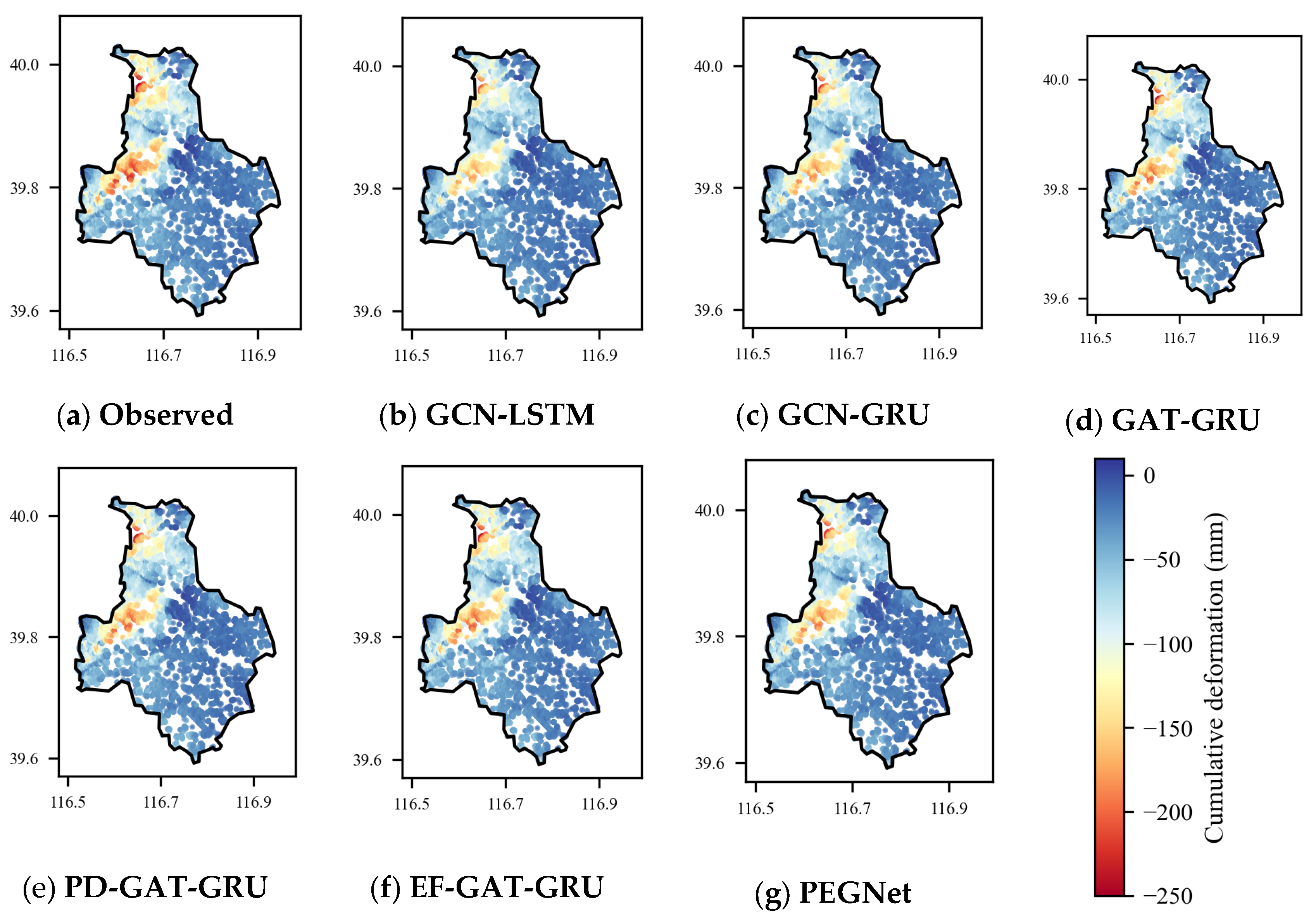
Figure A2.
Time series of cumulative deformation at three representative PS scatterers classified by annual subsidence rate: (a) severe ≥30 mm/yr, (b) moderate 10–30 mm/yr, and (c) slight ≤10 mm/yr, averaged across all six test windows. The x-axis spans 35 months from February 2020 to December 2022, with the first 24 months (from February 2020 to January 2022) serving as model input and the remaining 11 months (from February to December 2022) as the prediction period. Colored lines denote predictions from six model configurations; the black line denotes the observed values.
Figure A2.
Time series of cumulative deformation at three representative PS scatterers classified by annual subsidence rate: (a) severe ≥30 mm/yr, (b) moderate 10–30 mm/yr, and (c) slight ≤10 mm/yr, averaged across all six test windows. The x-axis spans 35 months from February 2020 to December 2022, with the first 24 months (from February 2020 to January 2022) serving as model input and the remaining 11 months (from February to December 2022) as the prediction period. Colored lines denote predictions from six model configurations; the black line denotes the observed values.
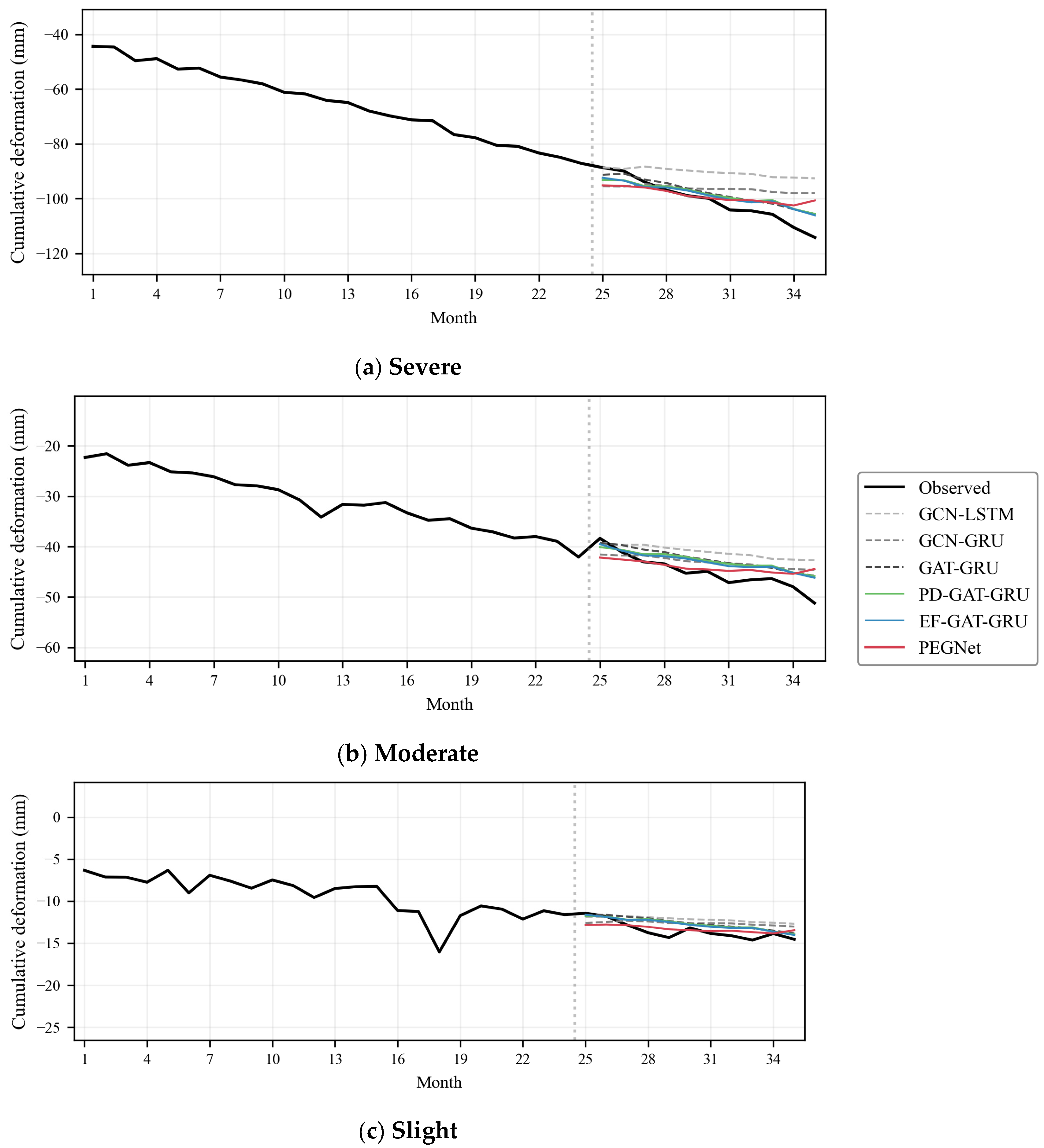

Table A3.
Per-step and overall RMSE (mm) of all models on the test set. The best value at each step is highlighted in bold.
Table A3.
Per-step and overall RMSE (mm) of all models on the test set. The best value at each step is highlighted in bold.
| Model | Step 1 | Step 2 | Step 3 | Step 4 | Step 5 | Step 6 | Overall |
|---|---|---|---|---|---|---|---|
| GCN-LSTM | 9.93 | 9.69 | 11.89 | 9.49 | 10.74 | 12.09 | 10.69 |
| GCN-GRU | 6.80 | 7.50 | 8.79 | 7.33 | 6.83 | 8.30 | 7.63 |
| GAT-GRU | 8.06 | 8.04 | 6.77 | 7.30 | 5.38 | 5.23 | 6.89 |
| PD-GAT-GRU | 6.47 | 5.93 | 4.69 | 8.82 | 6.61 | 4.54 | 6.34 |
| EF-GAT-GRU | 7.19 | 4.83 | 4.35 | 8.02 | 6.84 | 4.22 | 6.09 |
| PEGNet | 4.22 | 3.31 | 6.25 | 5.45 | 3.99 | 6.82 | 5.16 |
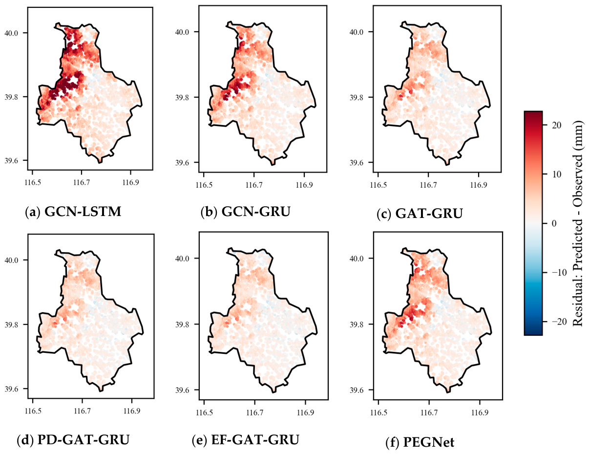
Figure A4.
Spatial distribution of residuals (predicted minus observed) for (a) GCN-LSTM, (b) GCN-GRU, (c) GAT-GRU, (d) PD-GAT-GRU, (e) EF-GAT-GRU, and (f) PEGNet, averaged over all six test windows at the last prediction step (from July 2022 to December 2022). Color scale is symmetric around zero.
Figure A4.
Spatial distribution of residuals (predicted minus observed) for (a) GCN-LSTM, (b) GCN-GRU, (c) GAT-GRU, (d) PD-GAT-GRU, (e) EF-GAT-GRU, and (f) PEGNet, averaged over all six test windows at the last prediction step (from July 2022 to December 2022). Color scale is symmetric around zero.
References
- Herrera-García, G.; Ezquerro, P.; Tomás, R.; Béjar-Pizarro, M.; López-Vinielles, J.; Rossi, M.; Mateos, R.M.; Carreón-Freyre, D.; Lambert, J.; Teatini, P.; Cabral-Cano, E.; Erkens, G.; Galloway, D.; Hung, W.-C.; Kakar, N.; Sneed, M.; Tosi, L.; Wang, H.; Ye, S. Mapping the global threat of land subsidence. Science 2021, 371, 34–36. [Google Scholar] [CrossRef] [PubMed]
- Bagheri-Gavkosh, M.; Hosseini, S.M.; Ataie-Ashtiani, B.; Sohani, Y.; Ebrahimian, H.; Morovat, F.; Ashrafi, S. Land subsidence: A global challenge. Sci. Total Environ. 2021, 778, 146193. [Google Scholar] [CrossRef] [PubMed]
- Chen, M.; Tomás, R.; Li, Z.H.; Motagh, M.; Li, T.; Hu, L.Y.; Gong, H.L.; Li, X.J.; Yu, J.; Gong, X.L. Imaging land subsidence induced by groundwater extraction in Beijing (China) using satellite radar interferometry. Remote Sens. 2016, 8, 468. [Google Scholar] [CrossRef]
- Fu, Y.Z.; Wang, J.L.; Zhang, Y.; Yang, H.L.; Li, L.; Ren, Z.Z. Spatiotemporal evolution of ground deformation in the Beijing Plain from 1992 to 2023 derived from a novel multi-sensor InSAR fusion method. Remote Sens. Environ. 2025, 319, 114635. [Google Scholar] [CrossRef]
- Zhou, C.D.; Tang, Q.H.; Zhao, Y.H.; Warner, T.A.; Liu, H.J.; Clague, J.J. Reduction of subsidence and large-scale rebound in the Beijing Plain after anthropogenic water transfer. Remote Sens. 2024, 16, 1528. [Google Scholar] [CrossRef]
- Meng, D.X.; Chen, B.B.; Gong, H.L.; Zhang, S.B.; Ma, R.; Zhou, C.F.; Lei, K.C.; Xu, L.W.; Wang, X.C. Land subsidence and rebound response to groundwater recovery in the Beijing Plain: A new hydrological perspective. J. Hydrol. Reg. Stud. 2025, 57, 102127. [Google Scholar] [CrossRef]
- Shi, M.; Gao, M.L.; Chen, Z.; Lyu, M.Y.; Gong, H.L.; Zhai, Y.Z.; Pan, Y. Land subsidence in Beijing: Response to the joint influence of South-to-North Water Diversion and ecological water recharge. GIScience Remote Sens. 2024, 61, 2315708. [Google Scholar] [CrossRef]
- Deng, Z.; Ke, Y.H.; Gong, H.L.; Li, X.J.; Li, Z.H. Land subsidence prediction in Beijing based on PS-InSAR and improved Grey-Markov model. GIScience Remote Sens. 2017, 54, 797–818. [Google Scholar] [CrossRef]
- Beck, H.E.; van Dijk, A.I.J.M.; de Roo, A.; Miralles, D.G.; McVicar, T.R.; Schellekens, J.; Bruijnzeel, L.A. Global-scale regionalization of hydrologic model parameters. Water Resour. Res. 2016, 52, 3599–3622. [Google Scholar] [CrossRef]
- Lyu, M.Y.; Ke, Y.H.; Guo, L.; Li, X.J.; Zhu, L.; Gong, H.L.; Constantinos, C. Change in regional land subsidence in Beijing after South-to-North Water Diversion observed using InSAR. GIScience Remote Sens. 2020, 57, 140–156. [Google Scholar]
- Lai, S.J.; Lin, J.X.; Dong, J.; Wu, J.Z.; Huang, X.L.; Liao, M.S. Investigating overlapping deformation patterns of the Beijing Plain by ICA of InSAR observations. Int. J. Appl. Earth Obs. Geoinf. 2025, 135, 104279. [Google Scholar]
- Ali, M.Z.; Chu, H.J.; Burbey, T.J. Mapping and predicting subsidence from spatio-temporal regression models. Hydrogeol. J. 2020, 28, 2865–2876. [Google Scholar]
- Lyu, M.Y.; Li, X.J.; Ke, Y.H.; Jiang, J.Y.; Zhu, L.; Guo, L.; Gong, H.L.; Chen, B.B.; Xu, Z.H.; Zhang, K.; Wang, Z.P. Reconstruction of spatially continuous time-series land subsidence based on PS-InSAR and improved MLS-SVR. GIScience Remote Sens. 2023, 60, 2230689. [Google Scholar] [CrossRef]
- Ikuemonisan, F.E.; Ozebo, V.C.; Olatinsu, O.B. Geostatistical evaluation of spatial variability of land subsidence rates in Lagos, Nigeria. Geod. Geodyn. 2020, 11, 316–327. [Google Scholar] [CrossRef]
- Shi, L.Y.; Gong, H.L.; Chen, B.B.; Zhou, C.F. Land subsidence prediction induced by multiple factors using machine learning. Remote Sens. 2020, 12, 4044. [Google Scholar] [CrossRef]
- Zhou, C.F.; Gong, H.L.; Chen, B.B. Prediction of land subsidence along Tianjin-Baoding railway using WT-RF. Remote Sens. Nat. Resour. 2021, 33, 34–42. [Google Scholar]
- Hochreiter, S.; Schmidhuber, J. Long short-term memory. Neural Comput. 1997, 9, 1735–1780. [Google Scholar] [CrossRef] [PubMed]
- Cho, K.; van Merriënboer, B.; Gulcehre, C.; Bahdanau, D.; Bougares, F.; Schwenk, H.; Bengio, Y. Learning phrase representations using RNN encoder-decoder. In Proceedings of the 2014 Conference on Empirical Methods in Natural Language Processing (EMNLP), Doha, Qatar, 25–29 October 2014. [Google Scholar]
- Veličković, P.; Cucurull, G.; Casanova, A.; Romero, A.; Lio, P.; Bengio, Y. Graph attention networks. In Proceedings of the 6th International Conference on Learning Representations (ICLR), Vancouver, BC, Canada, 24–28 April 2018. [Google Scholar]
- Kipf, T.N.; Welling, M. Semi-supervised classification with graph convolutional networks. In Proceedings of the 5th International Conference on Learning Representations (ICLR), Toulon, France, 24–26 April 2017. [Google Scholar]
- Navares, R.; Aznarte, J.L. Predicting air quality with deep learning LSTM. Ecol. Inform. 2020, 55, 101019. [Google Scholar] [CrossRef]
- Petty, T.R.; Dhingra, P. Streamflow hydrology estimate using machine learning (SHEM). J. Am. Water Resour. Assoc. 2018, 54, 55–68. [Google Scholar]
- Yu, B.; Yin, H.; Zhu, Z. Spatio-temporal graph convolutional networks: A deep learning framework for traffic forecasting. In Proceedings of the 27th International Joint Conference on Artificial Intelligence (IJCAI), Stockholm, Sweden, 13–19 July 2018. [Google Scholar]
- Karpatne, A.; Ebert-Uphoff, I.; Ravela, S.; Babaei, H.A.; Kumar, V. Machine learning for the geosciences: Challenges and opportunities. IEEE Trans. Knowl. Data Eng. 2019, 31, 1544–1554. [Google Scholar] [CrossRef]
- Liu, Q.H.; Zhang, Y.H.; Deng, M.; Wu, H.G.; Kang, Y.H.; Wei, J.J. Time series prediction of large-scale surface subsidence based on deep learning. Acta Geod. Et. Cartogr. Sin. 2021, 50, 396–404. [Google Scholar]
- Cao, X.Y.; Zhu, L.; Gong, H.L.; Guo, L.; Wei, Y.J.; Guo, T.; Chen, B.B.; Wang, H.G.; Li, H.J. Land subsidence simulation in the east of Beijing plain based on AM-LSTM. Natl. Remote Sens. Bull. 2022, 26, 1302–1314. [Google Scholar] [CrossRef]
- Peng, W.X.; Zhang, D.Y. Land subsidence prediction based on LSTM and Transformer: A case study of Shanghai. J. Spatio-Temporal Inf. 2024, 31, 94–103. [Google Scholar]
- Vaswani, A.; Shazeer, N.; Parmar, N.; Uszkoreit, J.; Jones, L.; Gomez, A.N.; Kaiser, Ł.; Polosukhin, I. Attention is all you need. In Advances in Neural Information Processing Systems; Long Beach, CA, USA, 4–9 December 2017; p. 30. [Google Scholar]
- Bergen, K.J.; Johnson, P.A.; de Hoop, M.V.; Beroza, G.C. Machine learning for data-driven discovery in solid Earth geoscience. Science 2019, 363, eaau0323. [Google Scholar] [CrossRef] [PubMed]
- Bauer, P.; Dueben, P.D.; Hoefler, T.; Quintino, T.; Schulthess, T.C.; Wedi, N.P. The digital revolution of Earth-system science. Nat. Comput. Sci. 2021, 1, 104–113. [Google Scholar] [CrossRef] [PubMed]
- Zhu, L.; Gong, H.L.; Li, X.J.; Zhou, C.F.; Ye, M.; Wang, H.G.; Zhang, K.; Han, M.M. Research progress and prospect of regional land subsidence. Hydrogeol. Eng. Geol. 2023, 51, 167–177. [Google Scholar]
- Raissi, M.; Perdikaris, P.; Karniadakis, G.E. Physics-informed neural networks. J. Comput. Phys. 2019, 378, 686–707. [Google Scholar] [CrossRef]
- Cuomo, S.; Di Cola, V.S.; Giampaolo, F.; Rozza, G.; Raissi, M.; Piccialli, F. Scientific machine learning through physics-informed neural networks. J. Sci. Comput. 2022, 92, 88. [Google Scholar] [CrossRef]
- Reichstein, M.; Camps-Valls, G.; Stevens, B.; Jung, M.; Denzler, J.; Carvalhais, N.; Prabhat, F. Deep learning and process understanding for data-driven Earth system science. Nature 2019, 566, 195–204. [Google Scholar] [CrossRef] [PubMed]
- Silling, S.A. Reformulation of elasticity theory for discontinuities and long-range forces. J. Mech. Phys. Solids 2000, 48, 175–209. [Google Scholar] [CrossRef]
- Silling, S.A.; Epton, M.; Weckner, O.; Xu, J.; Askari, E. Peridynamic states and constitutive modeling. J. Elast. 2007, 88, 151–184. [Google Scholar] [CrossRef]
- Zhang, K.; Gong, H.L.; Li, X.J.; Zhu, L.; Wang, C.; Chen, B.; He, J.; Guo, L.; Lyu, M.; Yan, Q.; Li, J. Application of peridynamic theory in regional land subsidence modeling. J. Geo-Inf. Sci. 2023, 25, 49–62. [Google Scholar]
- Zhu, L.; Li, J.T.; Gong, H.L.; Ye, M.; Dai, Z.; Li, X.; Teatini, P. Simulating earth deformation caused by groundwater pumping through ordinary state-based Peridynamics. J. Hydrol. 2024, 634, 131133. [Google Scholar] [CrossRef]
- Shen, H.F.; Zhang, L.P. Mechanism-learning coupling paradigms for parameter inversion and simulation in earth surface systems. Sci. China Earth Sci. 2023, 66, 568–582. [Google Scholar] [CrossRef]
- Holland, J.H. Emergence: From Chaos to Order, 1st ed.; Perseus Books: Cambridge, MA, USA, 1998. [Google Scholar]
- Tobler, W.R. A computer movie simulating urban growth in the Detroit region. Econ. Geogr. 1970, 46, 234–240. [Google Scholar] [CrossRef] [PubMed]
- Ferretti, A.; Prati, C.; Rocca, F. Permanent scatterers in SAR interferometry. IEEE Trans. Geosci. Remote Sens. 2001, 39, 8–20. [Google Scholar] [CrossRef]
- Wang, M.; Yao, J.; Chang, H.; Liu, R.; Cao, Y.; Zhao, Y. Monthly groundwater level grid dataset of China region (2005–2022). National Tibetan Plateau/Third Pole Environment Data Center. Available online: https://data.tpdc.ac.cn/en/data/96e53121-8c2e-419d-92e6-ff0e495087a3 (accessed on 29 July 2026).
- Xiong, Y.; Feng, W. Satellite gravity-based products for terrestrial water and groundwater storage changes in the China region (2002–2022). National Tibetan Plateau/Third Pole Environment Data Center. Available online: https://data.tpdc.ac.cn/en/data/7fe70fa6-5e34-497c-ac01-729c602e4663 (accessed on 29 July 2026).
- Peng, S.Z. 1-km monthly precipitation dataset for China (1901–2025). National Tibetan Plateau Data Center. Available online: https://data.tpdc.ac.cn/en/data/faae7605-a0f2-4d18-b28f-5cee413766a2 (accessed on 29 July 2026).
- Nash, J.E.; Sutcliffe, J.V. River flow forecasting through conceptual models part I — A discussion of principles. J. Hydrol. 1970, 10, 282–290. [Google Scholar] [CrossRef]
- Gupta, H.V.; Kling, H.; Yilmaz, K.K.; Martinez, G.F. Decomposition of the mean squared error and NSE performance criteria: A commentary on meaning and practical use. J. Hydrol. 2009, 377, 80–91. [Google Scholar]
Figure 1.
Study area and input features in Tongzhou District, Beijing. (a) Compressible layer thickness, faults, and district boundaries. (b)–(e) PS-InSAR, hydrogeological and meteorological data for January 2022: (b) cumulative deformation, (c) shallow groundwater level, (d) groundwater storage anomaly, and (e) precipitation.
Figure 1.
Study area and input features in Tongzhou District, Beijing. (a) Compressible layer thickness, faults, and district boundaries. (b)–(e) PS-InSAR, hydrogeological and meteorological data for January 2022: (b) cumulative deformation, (c) shallow groundwater level, (d) groundwater storage anomaly, and (e) precipitation.
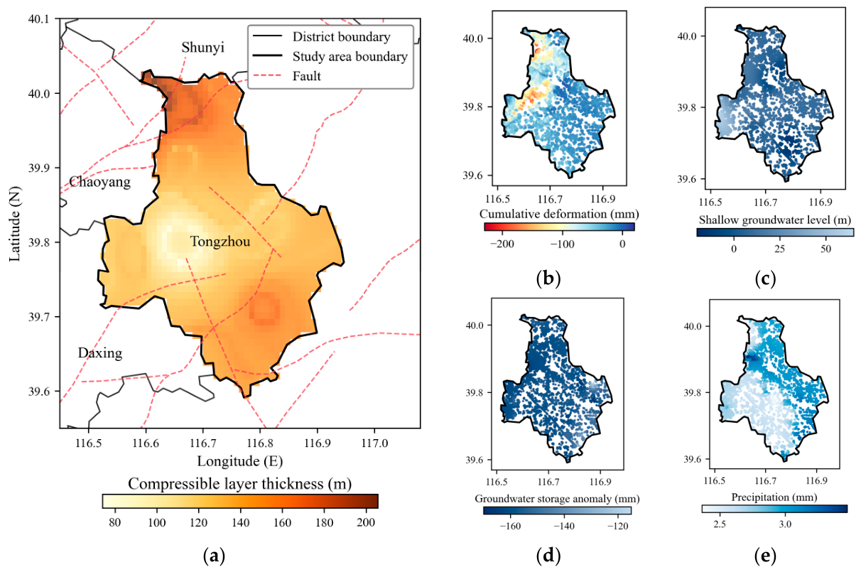
Figure 2.
Schematic diagram of the PEGNet framework. The Peridynamics gradient constraint (physics-based) and the emergent velocity features of subsidence are integrated into a four-stage spatio-temporal architecture.
Figure 2.
Schematic diagram of the PEGNet framework. The Peridynamics gradient constraint (physics-based) and the emergent velocity features of subsidence are integrated into a four-stage spatio-temporal architecture.
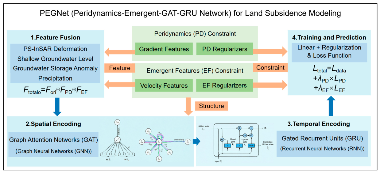
Figure 3.
Model performance comparison on the test set. Bars represent RMSE (blue) and MAE (red) with values annotated on the left y-axis. Overlaid markers represent NSE (green squares) and KGE (purple diamonds) referenced to the right y-axis. Models are ordered by architectural complexity, from the simplest temporal baseline (GCN-LSTM) to the full PEGNet framework.
Figure 3.
Model performance comparison on the test set. Bars represent RMSE (blue) and MAE (red) with values annotated on the left y-axis. Overlaid markers represent NSE (green squares) and KGE (purple diamonds) referenced to the right y-axis. Models are ordered by architectural complexity, from the simplest temporal baseline (GCN-LSTM) to the full PEGNet framework.
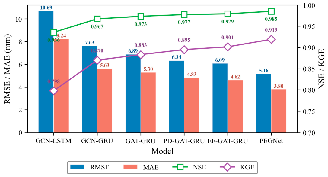
Figure 4.
Distribution of prediction errors for all six models. (a) Cumulative distribution function of absolute errors. (b) Probability density of raw errors (predicted minus observed). The CDF quantifies error magnitude, while the density plot reveals directional bias.
Figure 4.
Distribution of prediction errors for all six models. (a) Cumulative distribution function of absolute errors. (b) Probability density of raw errors (predicted minus observed). The CDF quantifies error magnitude, while the density plot reveals directional bias.
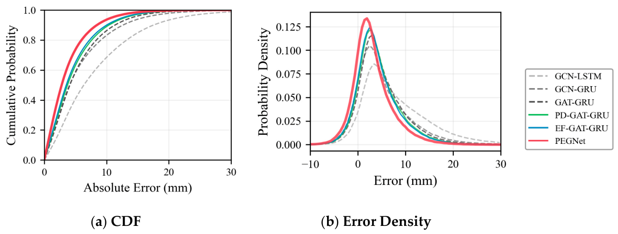
Figure 5.
Predicted versus observed cumulative deformation scatter density for all six models. Models are ordered from the simplest temporal baseline (GCN-LSTM) to the full PEGNet framework. Brighter colors indicate higher point density. Dashed red line denotes the 1:1 reference; solid blue line denotes the linear fit.
Figure 5.
Predicted versus observed cumulative deformation scatter density for all six models. Models are ordered from the simplest temporal baseline (GCN-LSTM) to the full PEGNet framework. Brighter colors indicate higher point density. Dashed red line denotes the 1:1 reference; solid blue line denotes the linear fit.
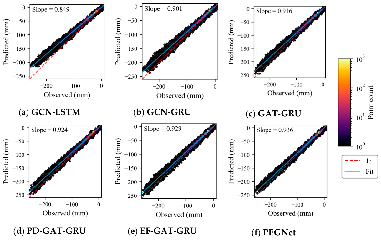
Figure 6.
Spatial distribution of cumulative deformation for (a) observed, (b) GCN-LSTM, (c) GCN-GRU, (d) GAT-GRU, (e) PD-GAT-GRU, (f) EF-GAT-GRU, and (g) PEGNet at the first prediction step (February 2022). Color scale is shared across all panels.
Figure 6.
Spatial distribution of cumulative deformation for (a) observed, (b) GCN-LSTM, (c) GCN-GRU, (d) GAT-GRU, (e) PD-GAT-GRU, (f) EF-GAT-GRU, and (g) PEGNet at the first prediction step (February 2022). Color scale is shared across all panels.
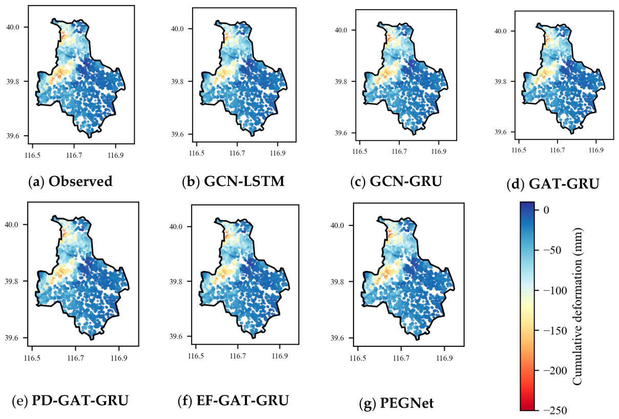
Figure 7.
Time series of cumulative deformation at three representative PS scatterers classified by annual subsidence rate: (a) severe ≥30 mm/yr, (b) moderate 10–30 mm/yr, and (c) slight ≤10 mm/yr. The vertical dashed line separates the 24-month input window (from February 2020 to January 2022, left) from the 6-month prediction period (from February 2022 to July 2022, right). Colored lines denote predictions from six model configurations; the black line denotes the observed values.
Figure 7.
Time series of cumulative deformation at three representative PS scatterers classified by annual subsidence rate: (a) severe ≥30 mm/yr, (b) moderate 10–30 mm/yr, and (c) slight ≤10 mm/yr. The vertical dashed line separates the 24-month input window (from February 2020 to January 2022, left) from the 6-month prediction period (from February 2022 to July 2022, right). Colored lines denote predictions from six model configurations; the black line denotes the observed values.
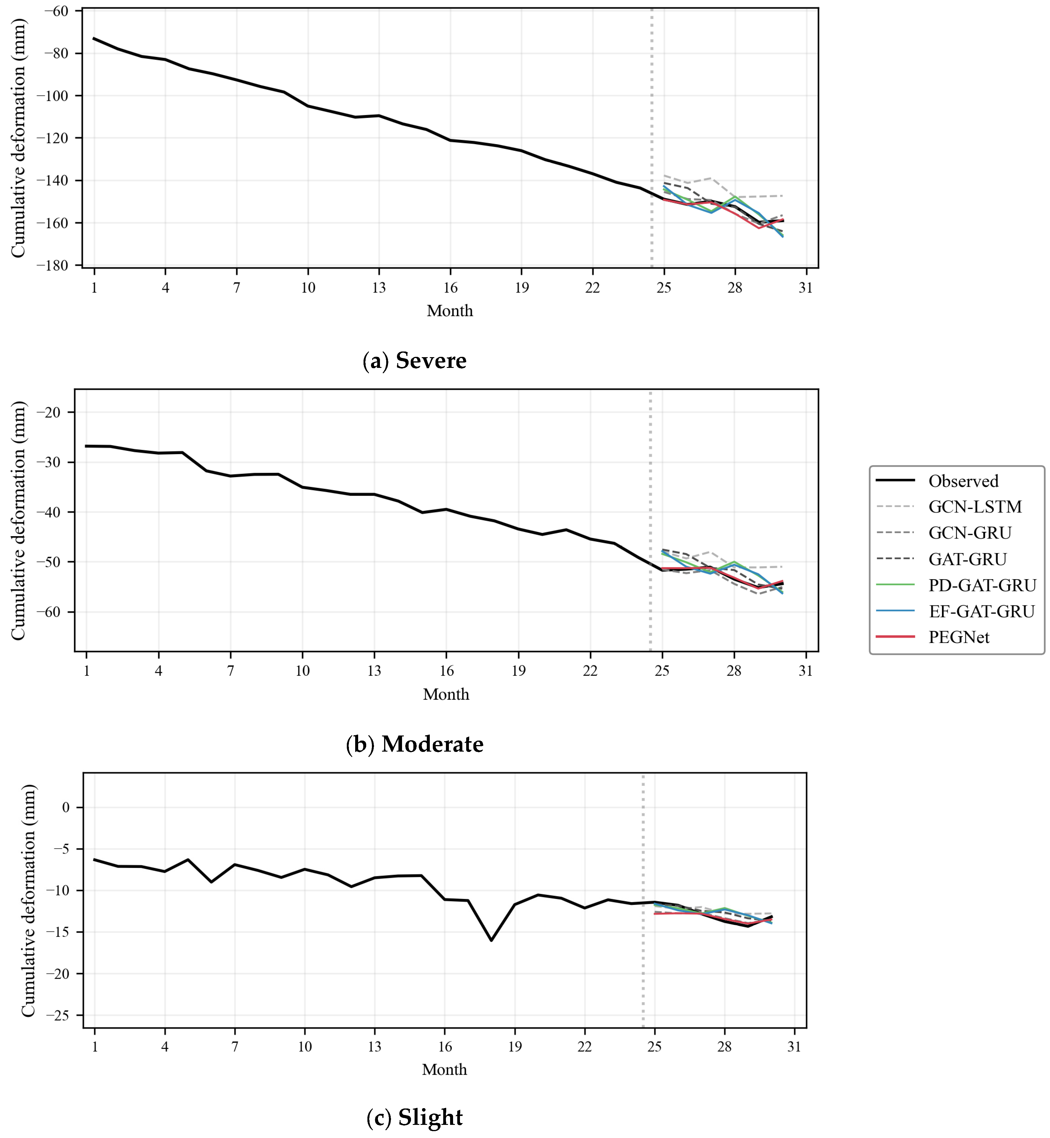
Figure 8.
Spatial distribution of per-point RMSE for (a) GCN-LSTM, (b) GCN-GRU, (c) GAT-GRU, (d) PD-GAT-GRU, (e) EF-GAT-GRU, and (f) PEGNet. Per-point RMSE is computed for each scatterer over the six prediction steps and then averaged across all scatterers.
Figure 8.
Spatial distribution of per-point RMSE for (a) GCN-LSTM, (b) GCN-GRU, (c) GAT-GRU, (d) PD-GAT-GRU, (e) EF-GAT-GRU, and (f) PEGNet. Per-point RMSE is computed for each scatterer over the six prediction steps and then averaged across all scatterers.
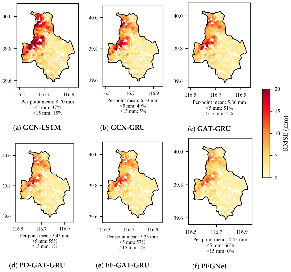
Figure 9.
Per-step RMSE comparison of all six models on the test set. Solid lines with markers indicate the RMSE at each prediction step.
Figure 9.
Per-step RMSE comparison of all six models on the test set. Solid lines with markers indicate the RMSE at each prediction step.
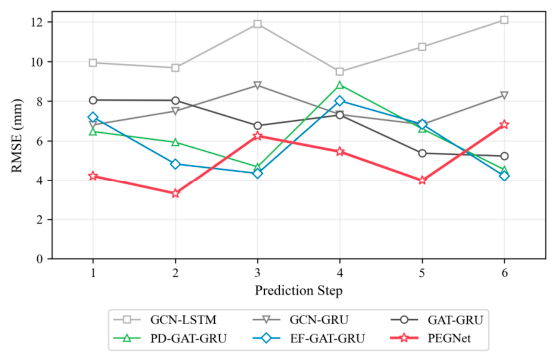
Figure 10.
Spatial distribution of residuals (predicted minus observed) for (a) GCN-LSTM, (b) GCN-GRU, (c) GAT-GRU, (d) PD-GAT-GRU, (e) EF-GAT-GRU, and (f) PEGNet, averaged over the first prediction step of all six test windows (covering from February 2022 to July 2022). Color scale is symmetric around zero.
Figure 10.
Spatial distribution of residuals (predicted minus observed) for (a) GCN-LSTM, (b) GCN-GRU, (c) GAT-GRU, (d) PD-GAT-GRU, (e) EF-GAT-GRU, and (f) PEGNet, averaged over the first prediction step of all six test windows (covering from February 2022 to July 2022). Color scale is symmetric around zero.
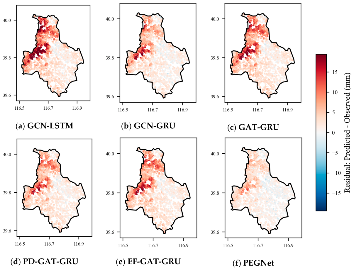
Table 1.
Sensitivity of validation RMSE (mm) to regularization weight combinations and . Values were obtained during hyperparameter tuning on the validation set. The optimal joint configuration is highlighted in bold.
Table 1.
Sensitivity of validation RMSE (mm) to regularization weight combinations and . Values were obtained during hyperparameter tuning on the validation set. The optimal joint configuration is highlighted in bold.
| Configuration | RMSE (mm) | ||
|---|---|---|---|
| PD-GAT-GRU (PD-only optimal) | 5.0 | 0.0 | 4.84 |
| EF-GAT-GRU (EF-only optimal) | 0.0 | 1.0 | 4.44 |
| PEGNet (naive combined) | 5.0 | 1.0 | 6.26 |
| PEGNet (PD dominant) | 5.0 | 0.2 | 5.23 |
| PEGNet (moderate weights) | 1.0 | 0.5 | 4.98 |
| PEGNet (best joint) | 0.5 | 0.2 | 4.16 |
Disclaimer/Publisher’s Note: The statements, opinions and data contained in all publications are solely those of the individual author(s) and contributor(s) and not of MDPI and/or the editor(s). MDPI and/or the editor(s) disclaim responsibility for any injury to people or property resulting from any ideas, methods, instructions or products referred to in the content. |
© 2026 by the authors. Licensee MDPI, Basel, Switzerland. This article is an open access article distributed under the terms and conditions of the Creative Commons Attribution (CC BY) license (http://creativecommons.org/licenses/by/4.0/).
Copyright: This open access article is published under a Creative Commons CC BY 4.0 license, which permit the free download, distribution, and reuse, provided that the author and preprint are cited in any reuse.