

Submitted:
30 July 2026
Posted:
31 July 2026
You are already at the latest version
Abstract
The critical-state branch of stress-fractional plasticity owes its analytical elegance to the Modified Cam-Clay surface, whose polynomial form admits closed-form Caputo gradients. We extend that elegance to the teardrop bounding surface of Chatwong et al., which is not polynomial in stress, by defining the operator as a Caputo derivative in the logarithm of normalized pressure, an orientation-corrected construction for that decreasing map (Section 2.3). On this axis the surface takes a power–exponential form, its critical-state terminal falls exactly at t* = 1/Ψ independently of Ω, and the fractional gradient reduces to incomplete-Beta–Kummer and Humbert-Φ₁ closed forms, verified against singularity-aware quadrature over 1,240 cases to relative errors below 10⁻¹¹. The resulting flow rule recovers associated flow (in the log-stress conjugate representation) as α → 1, and its flow vector coincides with the associated vector exactly at the critical state. Under the present endpoint-dependent hardening law and critical-state-dominated loading budget, substituting this operator for the fixed-window Grünwald–Letnikov flow of a companion factorial study collapses the dominant flow main effect from −60% to below 1% for both clays of the factorial study at every overconsolidation ratio tested, robustly across drained and approximately undrained proportional strain paths and conjugacy conventions — below 1% under the calibrated α(OCR) law, and within 2.5% across a constant-α sensitivity grid; the residual is a critical-state dwell transient, and the window semantics decide where fractional flow influence resides in a factorial design.
Keywords:
fractional plasticity
; ψ-Caputo derivative
; critical state
; bounding surface plasticity
; teardrop yield surface
; Humbert function
; closed-form solution
; non-associated flow
; factorial design
1. Introduction
Fractional-order plasticity entered soil mechanics along two connected lines: the fractional viscoplasticity of Sumelka [1,2,3], which generalized the direction of plastic flow to a non-local fractional gradient and showed that non-normality and induced plastic anisotropy follow from the operator itself [4], and the critical-state fractional flow rules of Sun, Shen and co-workers [5,6,7], developed across applications from ballast to bounding-surface, numerical-scheme and true-triaxial formulations [8,9,10,11,12,13] and extended to viscoplastic soils and anisotropically overconsolidated clay [14,15], with the dynamics of the fractional viscoplastic operator examined numerically in [16]; a related non-orthogonal flow-rule line was developed by Lu and co-workers [17]. In the classification of the recent review [18], these are the past-stress and future-critical-state branches of stress-fractional plasticity. The critical-state branch anchors the operator so that the integration limits are the current and the critical stress states, which merge as the critical state is approached [9], and demonstrated — for the Modified Cam-Clay (MCC) surface [19] within the critical-state framework [20] — that state-dependent non-associativity then emerges without any plastic potential [9,11]. The analytical appeal of that line rests on a specific coincidence: MCC is polynomial in linear stress, so its Caputo fractional gradients reduce to incomplete Beta and Gamma functions in closed form [9,18].
The companion study [21] embedded a fractional flow operator in a 2×2×2 factorial with the teardrop bounding surface of Chatwong et al. [22] and a nonlinear AJOP compression law [23], and found the flow factor to be the single largest main effect (≈ −60% of the baseline plastic volumetric response at OCR = 5 for two independently calibrated clays). That study was, however, deliberately explicit that its operator was a fixed-window, past-stress Grünwald–Letnikov (GL) scheme — a loading-memory semantics in the past-stress branch of [18] — and not the critical-state Caputo definition [9], which it retained as motivation only. Two questions follow immediately. First, can the critical-state Caputo operator be constructed exactly for the teardrop surface at all, given that the surface is not polynomial in linear stress? Second, do the factorial conclusions of the companion study survive the change of window semantics?
This paper answers both. The first answer is a closed form: on the log-stress axis — formally, a Caputo derivative taken with respect to another function [24], here the logarithm, in the weighted/conjugated sense of [25] — the teardrop takes a power–exponential form, its critical-state terminal is exactly the reciprocal shape parameter, and its Caputo gradient is an incomplete-Beta–Kummer or Humbert-Φ1 expression — the same class of special functions that made the MCC results attractive, now on a surface those results cannot reach. The second answer is a collapse: with the critical-state operator in place, the dominant flow main effect of the companion study falls below 1% at every tested state, for both soils and both loading paths, and is shown to be a transient that vanishes as the state reaches and dwells at the critical state. The contributions are: (i) the exact critical-state terminal t* = 1/Ψ and the closed-form Caputo gradients of the teardrop (Section 2), verified to near machine precision; (ii) a flow rule built on them that is exactly associated at the critical state (Section 2.3); (iii) a paired factorial re-evaluation showing the collapse of the flow main effect and its migration into the geometry×flow interaction (Section 4); and (iv) a clean discriminant between the two available routes to state-dependent non-associativity (Section 5).
Relation to the companion study, stated plainly: the calibrated parameters, path definitions, hardening semantics, factorial index definitions and the self-testing reference implementation are inherited from [21] to guarantee one-to-one comparability. Everything else is new to this paper: the operator belongs to the other branch of stress-fractional plasticity (critical-state window semantics rather than past-stress memory [18]); the closed-form ψ-Caputo gradients, the exact terminal t* = 1/Ψ and their 1,240-case verification are new analytical results; the principal numerical finding reverses the headline of [21]; and the dwell mechanism, the endpoint identity and the phase-transformation discriminant are new. The companion is the control experiment for this paper, not its template.
2. Closed-Form Critical-State Caputo Flow for the Teardrop
2.1. The Teardrop in Log-Stress Space and Its Exact Critical-State Terminal
In normalized triaxial space the teardrop yield curve of Chatwong et al. [22] is = g() = ·(Ω ln(1/))1/Ψ, with = p′/p′c, = q/(Mp′c) and shape parameters Ψ, Ω, where M is the critical-state stress ratio of Table 2. All stresses and dilatancies are hereafter M-normalized in this sense — η̅ = η/M and D̅ = D/M, equivalently M ≡ 1 in the canonical implementation (ff_canonical.py in Supplementary S1) — with physical values recovered as η = Mη̅ and D = MD̅; bars mark the normalized stress variables, while the dilatancy symbols D, D_int, D_cap and D_GL denote M-normalized values throughout. Substituting the log-stress variable t = ln(1/) gives
a power–exponential form: the algebraic component (Ωt)1/Ψ is a pure power of t — the substitution = e−t converts the logarithmic composition into this power — while the factor e−t is the exponential image of itself; it is precisely this structure (power × exponential against the Caputo kernel) that renders every required integral closed-form — the log-stress axis being the natural axis of soil compression, on which the classical and AJOP compression laws are themselves defined [19,20,23]. The critical state of the surface — the apex, at which the associated flow direction is purely deviatoric — satisfies dg̃/dt = 0, which reduces to Ω t = Ω/Ψ, i.e.,
g̃(t) = e−t · (Ω t)1/Ψ, t ≥ 0,
For the four soils of the companion calibration this gives * = 0.490 (Ψ=1.4, Boston Blue and London Clay), 0.513 (Ψ=1.5, kaolin) and 0.386 (Ψ=1.05, Lower Cromer Till). We verified the closed form against direct numerical maximization to 10−8 for Ψ ∈ [1.05, 2.0]. This point is a property of the surface (the associated-flow critical state) and must not be confused with the zero of the embedded non-associated rule of [22], which lies at ≈ 0.341 for the Boston Blue Clay shape (Section 5).
2.2. Closed-Form Caputo Integrals
With f(t) = 0 − g̃(t) at fixed 0 (the Caputo construction annihilates the constant), the fractional gradient — in the classical Caputo sense [26,27,28] — requires integrals of g̃′(s) = e−s·Ω1/Ψ·[(1/Ψ)s1/Ψ−1 − s1/Ψ] against the kernel |x−s|−α, i.e., two instances of the master integral with β = 1/Ψ and β = 1/Ψ − 1. For the tip terminal (a = 0) the master integral is classical (entry 3.383.1 of [29]):
∫0ᵗ sβ e−s (t−s)−α ds = B(β+1, 1−α) · tβ+1−α · 1F1(β+1; β+2−α; −t).
For the critical-state terminal a = t* > 0 we derived the shifted forms by the substitution s = a + (x−a)u and identification with the Euler-type integral representation of the Humbert confluent hypergeometric function Φ1 [30,31]:
dry side (x > a): ∫ₐˣ sβ e−s(x−s)−α ds = aβ e−a (x−a)1−α/(1−α) · Φ1(1, −β; 2−α; −(x−a)/a, −(x−a)),
wet side (x < a): ∫ₓᵃ sβ e−s(s−x)−α ds = xβ e−x (a−x)1−α/(1−α) · Φ1(1−α, −β; 2−α; −(a−x)/x, −(a−x)).
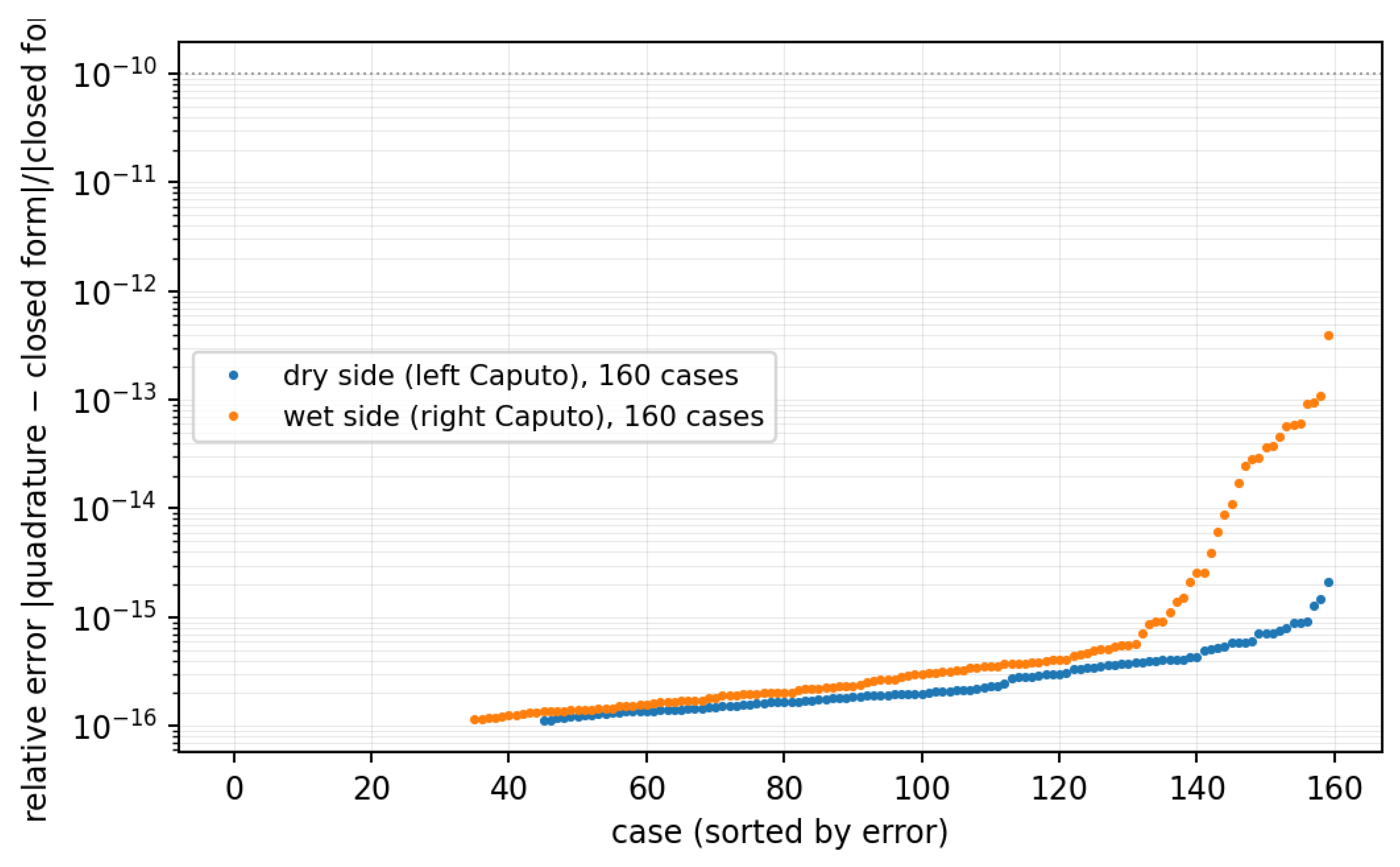
Φ1 was evaluated by its single-series expansion in the exponential variable with Gauss 2F1 factors, which remains valid under the analytic continuation of 2F1 for the parameter regimes encountered here (first argument down to −2.3). Verification against singularity-aware weighted quadrature [32] covered 400 cases for the tip-terminal form (3) over the teardrop exponents γ ∈ {1/Ψ − 1, 1/Ψ} (worst relative error 1.2×10⁻¹⁵), 200 cases at a second shifted terminal a = ln 2 in the moderate-|Z| regime with representative exponents γ ∈ {0.4, 0.7, 1.0, 1.5} (worst 7.4×10⁻¹⁶), and 640 cases for the critical-state terminal spanning both sides, both companion critical states, Ψ ∈ [1.05, 2.0] and α ∈ [0.3, 0.95] (worst 5.1×10⁻¹²); the a = ln 2 block stress-tests the master integrals at an additional shift value and is distinct from the dilatancy of the classical geometry, which is obtained from quadrature tables (Section 3.1). Figure 2 shows the full error distribution of a 320-case subset regenerated for this paper.
2.3. Flow Rule and Its Limits
The operator is defined as the terminal-directed, orientation-corrected Caputo operator in the log-stress coordinate t = −ln , taken toward the critical-state terminal t* = 1/Ψ (Section 2.2). It may equally be written as an orientation-corrected extension of the ψ-Caputo construction of Almeida [24] for the decreasing map ψ() = ln(1/): the kernel that keeps the integrand real and positive is the orientation-corrected form (ψ()−ψ(u))−α on the dry side (t > t*) and (ψ(u)−ψ())−α on the wet side (t < t*), rather than the increasing-ψ kernel of [24]. The two forms carry identical information: under u = e−s the change of variable maps the Caputo integral in t onto this ψ-Caputo integral in , and as α → 1 the operator returns dF/dt = − f′(), i.e., associated flow in the log-stress (t–q) conjugate representation. The choice ψ = ln(1/) is the modeling postulate, argued from the fact that soil compression laws — classical and AJOP alike — are native to the logarithmic stress axis [19,20,23]. In the variable t = ψ() these are exactly the terminal-directed, orientation-corrected Caputo operators of Section 2.2, which is how the closed forms arise. The flow vector is assembled as follows. The yield function f(,) = − g() is linear in , so its deviatoric flow component is the integer derivative ∂f/∂ = 1, left untouched; the volumetric component replaces ∂f/∂ψ (the log-conjugate volumetric direction, work-paired with the increment d ln ) by the terminal-directed, orientation-corrected Caputo operator of Proposition 1, left-sided on the dry side (t > t*) and right-sided on the wet side (t < t*). The Caputo construction annihilates the constant 0, so only integrals of g̃′ appear. The reported dilatancy is the component ratio Dcap = (volumetric)/(deviatoric) in this convention. The transformation to the -conjugate pairing is stated with its sign: dψ/d = −1/ = −et, so the covector components obey ∂f/∂ = −et·∂f/∂ψ; because Dcap is built from g̃′ = −f′, the -conjugate dilatancy is D̅p̅ = −et·Dcap: the factor −e^t < 0 is an orientation-reversing rescaling, converting the dilative-positive t-conjugate convention of Proposition 1 to the contractive-positive convention of the evolution equations while moving no zero; the physical dilatancy then follows as D = M·D̅_p̅, where M ≡ 1 in the normalized coordinates used throughout. Rescaling the flow magnitude does, however, alter the stress path and the hardening evolution en route, so convention-independence of the accumulated response is not a corollary of the zero analysis alone; it follows instead from an endpoint identity: the hardening law ties the increments exactly, dεvp = λeff(p′c)·d ln p′c, so the accumulated plastic volumetric strain of any converged configuration equals ∫ λeff d ln p′c between the initial and terminal states — a function of the endpoints only, independent of the dilatancy magnitude en route. Stated with its conditions: under the present hardening law and loading/convergence conditions, two configurations that reach the same absolute terminal state accumulate the same plastic volumetric response, irrespective of the path-dependent dilatancy magnitude and of the conjugacy convention. On the constant-p′ path used here, sharing the normalized terminal * does fix the absolute terminal, p′c* = p′/*, so the condition is met by construction; for other loading controls the coincidence of absolute terminals must be established rather than assumed. The GL window differs precisely because its effective terminal is displaced. The rerun confirms the identity in the cases checked: re-running the full Caputo factorial in the -conjugate convention leaves every flow-independent index unchanged and reduces the flow main effect to a numerically-zero contrast at OCR = 5 (|ΔF| < 0.1% of baseline for both soils; the exact last digit of such a near-zero contrast is floating-point-ordering dependent across platforms and is not a determinism target), while the terminal states of the integer and Caputo classical configurations agree to three decimals ( = 0.4996 versus 0.5000, accumulated strain −0.1375 versus −0.1377). Reported magnitudes of Dcap remain convention-specific and are labelled as such.
Proposition 1 (Closed-form critical-state Caputo flow). Let , with critical-state terminal , exponent and constant , so that and with . The volumetric flow component is , where is the terminal-directed, orientation-corrected Caputo operator toward — left-sided for , right-sided for , with the orientation sign fixed so that its integer limit is the associated dilatancy on both sides (deviatoric component ; the constant is annihilated). Then
with and the Humbert confluent function. For every fixed t > 0, the expressions are real-valued and finite in closed form for all , (including ); they diverge only in the endpoint limit t → 0+. Moreover , so the flow is purely deviatoric at the critical state for every ; and as , on both sides , the integer associated dilatancy in the -conjugate representation — dilative on the dry side, contractive on the wet side. As () both and diverge in step, reflecting the vertical surface tangent at the isotropic axis; this limit lies outside the loading paths, which remain in . The -conjugate dilatancy is , an orientation-reversing rescaling that preserves the zero at and returns the contractive-positive convention; the physical dilatancy follows as D = M·D̅_p̅(t), with M ≡ 1 in the present normalized coordinates.
Proof. Since is linear in , . Substituting into the terminal-directed integrals and evaluating term by term with the master integrals (4)–(5) at , and gives the stated forms (6) and (7); the common leading sign on both sides is fixed by the orientation correction, so that throughout.
Three structural properties were verified numerically (Figure 1). (i) As α → 1−, Dcap converges to the integer associated dilatancy at every tested state (seven states, agreement to the third decimal at α = 0.999). (ii) Associativity at the critical state, stated precisely: at t = t* both the ψ-Caputo volumetric component (its integration interval having shrunk to zero) and the integer volumetric gradient vanish, while the deviatoric components coincide identically; the full flow vector of the fractional rule therefore equals the associated flow vector — purely deviatoric — exactly at the critical state, for every α, and Dcap changes sign across it (contractive on the wet side, dilative on the dry side). In any neighbourhood of the critical state the two directions differ (the claim is exact coincidence at the terminal, not in its vicinity) — the defining property the fixed-window GL operator lacks, since its window remains finite at the critical state. (iii) The induced non-associativity is strongly non-uniform: at α = 0.641 the ratio Dcap/Dassoc ranges from ≈ 0.37 near the critical state to ≈ 1.13 far on the dry side, a richer structure than any uniform scaling.
Figure 2.
Verification of the closed forms: relative error between the Humbert-Φ1 expressions and singularity-aware weighted quadrature over 320 parameter cases (both sides, Ψ ∈ [1.05,2.0], α ∈ [0.3,0.95]). All cases fall below 10−11; the full 1,240-case grid of Section 2.2 attains a worst relative error of 5.1×10⁻¹².
Figure 2.
Verification of the closed forms: relative error between the Humbert-Φ1 expressions and singularity-aware weighted quadrature over 320 parameter cases (both sides, Ψ ∈ [1.05,2.0], α ∈ [0.3,0.95]). All cases fall below 10−11; the full 1,240-case grid of Section 2.2 attains a worst relative error of 5.1×10⁻¹².
3. Numerical Setup
3.1. Constitutive Equations and State Variables
For self-containment the governing relations of the companion study [21,22] are summarised here in the normalized coordinates used throughout, identical to those of Section 2: and ; the normalized stress ratio and dilatancy are η̅ = η/M and D̅ = D/M (physical values η = Mη̅, D = MD̅; the canonical implementation sets M ≡ 1 in these coordinates). . Its integer flow is the integer-order embedded non-associated rule of [22] — not the associated gradient of the locus —
The fixed-window Grünwald–Letnikov operator of [21] applies the same window to the locus function ,
an additive window in with binomial weights ; the critical-state Caputo dilatancy is that of Proposition 1. The AJOP compression law [23] sets the compression slope from the current preconsolidation pressure,
with per-soil from [23] (p_r denotes the AJOP reference pressure, relabelled from the source symbol to avoid clashing with the response R). The effective hardening modulus is , with for the AJOP-compression configurations and the constant for the conventional ones; a configuration is hardening-singular — its response undefined and reported as such rather than clamped — when . The fractional order is state-dependent and frozen at the initial state,
a modeling assumption retained for comparability with [21]. Along a drained, constant-, shear-strain-controlled path the state and the response (the M-normalized accumulated plastic volumetric response; the corresponding physical accumulated plastic volumetric strain is R_phys = MR) evolve as
while the approximately-undrained path integrates with . Here is a dimensionless numerical loading budget, not a physical strain target: it is set to — far beyond any laboratory strain — solely to drive every configuration through the critical-state dwell, so that the accumulated-response comparison is taken at a common, fully-developed terminal. The dilatancy D entering these evolution equations is the M-normalized quantity of Section 2.1 (M ≡ 1), so the computed response is likewise M-normalized, R_phys = MR; because all factorial contrasts are normalized by the within-soil baseline, the common factor M cancels identically from every within-soil percentage index; it also leaves equilibrium locations unchanged, because a positive rescaling does not move any dilatancy zero. The drained factorial tables use 30,000 increments (the sweep of record); a 60,000-increment rerun verifies refinement, and the approximately undrained runs use 200,000 increments.
Beyond the constitutive relations of Section 3.1, the numerical machinery follows the companion study [21]: the locked Level-I parameter set (Table 2) [21,22], the incremental drained (constant-p′, shear-strain-controlled, budget εₛᵖ = 6) and approximately undrained paths, the state-dependent fractional order α(OCR) with αmin = 0.55 and k = 0.40 (a modeling assumption, retained for comparability with [21]), the hardening-singularity semantics in which singular configurations raise and are reported as undefined rather than clamped, and the 42-check self-testing reference implementation. The critical-state Caputo dilatancy enters as a third flow level alongside the integer and GL-window operators. Because Φ1 evaluation per step is costly, Dcap() is precomputed on Hölder-aware per-side splines in the variable w = |t − t*|1−α, which removes the (t−t*)1−α kink at the critical state; the interpolation error is ≤ 2.4×10⁻⁸ against exact evaluation, and a full path integrated on the table agrees with a path integrated on exact per-step evaluation to 1.2×10⁻¹³ in accumulated strain. The classical reference geometry (the normalized MCC-type surface [19]), whose log-stress form is not a power law, receives its critical-state Caputo dilatancy (terminal t* = ln 2) by the same table machinery built on singularity-aware quadrature; the closed form is a property of the teardrop and is presented as such.
The design is presented as paired 2×2×2 factorials sharing the integer-flow baseline: the pairing {integer ↔ GL-window} reproduces the companion study [21] exactly, and the pairing {integer ↔ Caputo-CS} is new, with configurations C0–C7 mirroring F0–F7. This preserves one-to-one comparability of every index. For self-containment: with R denoting the M-normalized accumulated plastic volumetric response of a configuration and b = |R(C0)|, the indices are ΔG = (R(C1)−R(C0))/b, ΔF = (R(C2)−R(C0))/b, ΔC = (R(C3)−R(C0))/b, the pairwise interactions the standard 2×2 contrasts (e.g., IGF = (R(C4)−R(C2)−R(C1)+R(C0))/b), and IGFC the triple contrast; simple effects quoted below are geometry-conditional flow contrasts such as ΔF|teardrop = (R(C4)−R(C1))/b = ΔF + IGF.

Table 1.
Configurations of the Caputo pairing (mirroring F0–F7 of the companion).
| Config | Yield geometry | Flow operator | Hardening/compression |
|---|---|---|---|
| C0 | Classical | Integer-order | Conventional (λ) |
| C1 | Teardrop | Integer-order (embedded rule of [22]) | Conventional (λ) |
| C2 | Classical | Caputo–CS | Conventional (λ) |
| C3 | Classical | Integer-order | AJOP [23] |
| C4 | Teardrop | Caputo–CS | Conventional (λ) |
| C5 | Teardrop | Integer-order | AJOP [23] |
| C6 | Classical | Caputo–CS | AJOP [23] |
| C7 | Teardrop | Caputo–CS | AJOP [23] |
Table 2.
Locked Level-I parameter set of the companion study [21] (single set, whole program; identical to its published Supplementary S2; soil sources as compiled in [21,22]). The λ and κ listed here are the source-calibration constants of [22]; the integrator takes their ratio κ/λ and applies it to the AJOP-consistent compression index of [21], giving λ = 0.187, κ = 0.0365 for Boston Blue Clay and λ = 0.0586, κ = 0.0223 for London Clay. The normalized constant-λ indices are independent of λ − κ. The factorial uses Boston Blue Clay and London Clay; kaolin and Lower Cromer Till complete the calibration record. The critical-state ratio M enters the analysis only through the normalization of Section 2.1 and the recovery of physical quantities (η = Mη̅, D = MD̅).
Table 2.
Locked Level-I parameter set of the companion study [21] (single set, whole program; identical to its published Supplementary S2; soil sources as compiled in [21,22]). The λ and κ listed here are the source-calibration constants of [22]; the integrator takes their ratio κ/λ and applies it to the AJOP-consistent compression index of [21], giving λ = 0.187, κ = 0.0365 for Boston Blue Clay and λ = 0.0586, κ = 0.0223 for London Clay. The normalized constant-λ indices are independent of λ − κ. The factorial uses Boston Blue Clay and London Clay; kaolin and Lower Cromer Till complete the calibration record. The critical-state ratio M enters the analysis only through the normalization of Section 2.1 and the recovery of physical quantities (η = Mη̅, D = MD̅).
| Soil | λ | κ | ν | M | e0 | Ω | Ψ | n policy |
|---|---|---|---|---|---|---|---|---|
| Boston Blue Clay | 0.184 | 0.036 | 0.10 | 1.353 | 2.059 | 0.93 | 1.4 | n = 0.5+2/OCR (fixed at initial OCR) |
| Kaolin Clay | 0.26 | 0.05 | 0.20 | 0.896 | 2.957 | 1.17 | 1.5 | monotonic decreasing (n ≤ 4) |
| London Clay | 0.168 | 0.064 | 0.25 | 0.827 | 1.843 | 1.23 | 1.4 | n = 0.5+2/OCR (fixed at initial OCR) |
| Lower Cromer Till | 0.063 | 0.018 | 0.30 | 1.20 | 0.747 | 0.97 | 1.05 | monotonic decreasing |
The last column of Table 2 states each soil’s hardening-exponent policy in words; Table 3 gives the numerical exponent n it produces, each entry written as n (OCR) — the exponent value with its overconsolidation ratio in parentheses — at the ratios used in the analysis. For Boston Blue Clay and London Clay n follows n = 0.5 + 2/OCR, fixed at the initial OCR (convention B); for kaolin and Lower Cromer Till the exponent is instead held monotonically decreasing with OCR under the per-soil cap n ≤ 4.
Table 3.
Hardening exponent n used in the analysis (locked set), each entry n (OCR). Boston Blue Clay and London Clay follow the n–OCR convention of [22] at fixed initial OCR (convention B); kaolin and Lower Cromer Till are monotonically decreasing under the per-soil cap n ≤ 4.
Table 3.
Hardening exponent n used in the analysis (locked set), each entry n (OCR). Boston Blue Clay and London Clay follow the n–OCR convention of [22] at fixed initial OCR (convention B); kaolin and Lower Cromer Till are monotonically decreasing under the per-soil cap n ≤ 4.
| Soil | n (OCR) | |||||||
|---|---|---|---|---|---|---|---|---|
| Boston Blue Clay | 2.5(1.0) | 1.5(2.0) | 1.0(4.0) | 0.74(8.5) | ||||
| London Clay | 2.5(1.0) | 1.5(2.0) | 0.83(6.0) | 0.61(18.7) | ||||
| Kaolin Clay | 4.0(1.0)† | 4.0(1.2) | 4.0(1.4) | 4.0(1.8) | 3.1(2.5) | 3.1(3.0) | 2.25(4.5) | 2.1(6.4) |
| Lower Cromer Till | 4.0(1.0)† | 4.0(2.0) | 0.45(4.1) | 0.45(9.7) | ||||
† At OCR = 1 the exponent is unidentifiable (the spacing ratio → 1); the per-soil cap value is adopted.
4. Results: Collapse and Migration of the Flow Effect
4.1. The Flow Main Effect Collapses
Table 4 reports the paired factorial at OCR = 5, with the GL-window column reproducing the companion study [21]. Replacing the GL-window flow by the critical-state Caputo flow leaves every flow-independent index unchanged to the reported precision (ΔG, ΔC, IGC — an internal consistency check of the pairing) and collapses the flow main effect from −60.25% to +0.69% of |R(C0)| for Boston Blue Clay and from −60.32% to +0.10% for London Clay; the flow×compression interaction collapses equally (+41.70% → −0.60%; London: undefined → +0.13%). All tabulated values use n = 30,000 increments (the sweep of record); at n = 60,000 the Boston Blue Clay value moves only from +0.689% to +0.679%, and the near-zero London flow×compression contrast from +0.13% to +0.06%, i.e., within discretisation noise of contrasts that are numerically zero. Across the full OCR sweep (Table 5, Figure 4) the collapsed ΔF never exceeds 1.0% for either soil, against −37% to −115% for the GL window. The result is path-robust: under the approximately undrained path at OCR = 5, ΔFcap = 0.001% (BBC) and 0.000% (London). It is also robust to the assumed fractional-order law: replacing α(OCR) by constant α = 0.55 or 0.75 across a 12-point grid (both soils, OCR = 3, 5, 10) leaves the collapse intact everywhere, with |ΔFcap| ≤ 2.5% and the largest residual (+2.47%, Boston Blue Clay, OCR = 3, α = 0.55) occurring exactly where the mechanism predicts — the most strongly non-local operator on the longest approach path — and falling below 0.3% at α = 0.75.
4.2. The Collapse Is a Critical-State Dwell Effect
Figure 3 resolves the mechanism. At small imposed shear budgets — before the state reaches the critical state — the Caputo and integer flows differ strongly and ΔFcap is large (+71% at budget 0.2 for BBC); as the budget grows and the state dwells at the critical state, where the Caputo flow is exactly associated and shares the integer terminal, ΔFcap decays monotonically toward zero (+3.9% at budget 3, +0.7% at budget 6). London Clay, whose states reach the critical state faster, decays faster (below 1% already at budget 1.5). The companion study [21] showed that its classical configuration spends 96–100% of the imposed budget traversing the band between the two flow rules’ critical-state points, while its teardrop configuration reaches its own critical state early and remains there for the rest of the budget; in both cases the path dwells at or beside the critical state, where the GL window retains finite non-associativity and therefore accumulates its −60%, while the critical-state-anchored operator cannot. The dominant fractional flow main effect of the companion study is thereby identified as a critical-state-displacement effect of the window semantics — exactly the kind of operator-specific property that study cautioned about [21], now quantified.
4.3. The Flow Effect Migrates into the Geometry×Flow Interaction
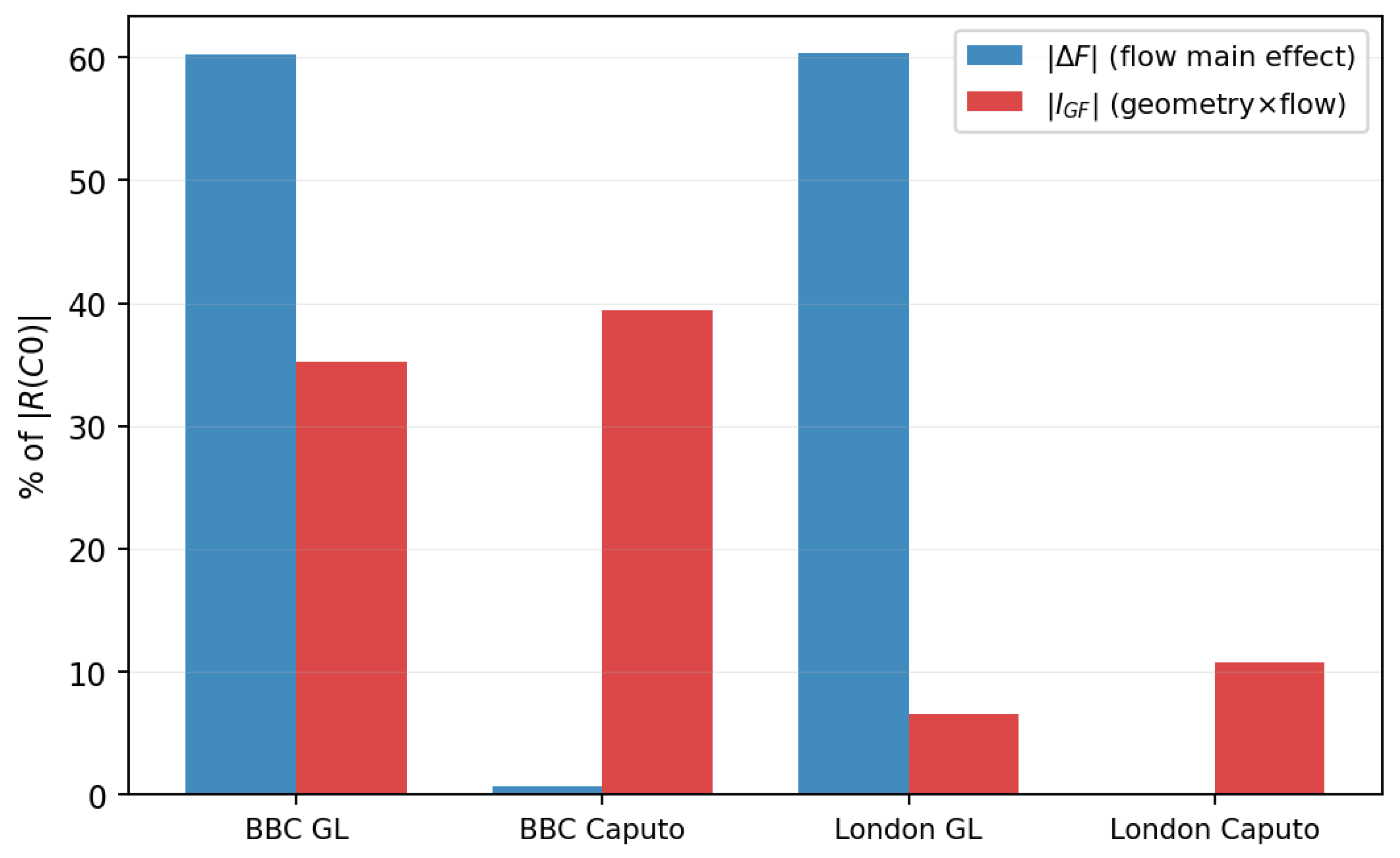
The flow operator does not become irrelevant. The least interpretation-laden statement uses simple effects: at OCR = 5 for Boston Blue Clay, the simple effect of replacing the integer by the Caputo-CS flow is +0.69% on the classical geometry but −38.8% on the teardrop (London: +0.10% versus −10.7%), whereas under the GL window it is large on both geometries (−60.2% and −95.5% for BBC; −60.3% and −66.9% for London). Under the critical-state operator the flow effect is therefore strongly geometry-dependent — on the teardrop the Caputo flow (critical state at * = 0.490) and the embedded rule of [22] (crossing at 0.341) disagree about where dilation stops, while on the classical reference the two flows share the terminal and nearly coincide — and in factorial bookkeeping this expresses itself as a dominant geometry×flow interaction, IGF = −39.5% (BBC) and −10.8% (London), of the same magnitude as and opposite sign to ΔG (Figure 5). We use ‘migration’ only in this bookkeeping sense: main effects and interactions depend on the coding and reference level of the design, and the invariant content is the geometry-conditional simple effects just quoted. The three-way interaction rises accordingly (IGFC up to +18% for BBC). A practical corollary concerns the hardening singularity of the companion study [21]: because the Caputo-flow configurations follow different stress paths, London Clay AJOP-compression configurations remain regular through OCR = 6 where their GL counterparts were already undefined, and the singular exposure re-enters only at OCR ≥ 7 through the compression factor itself (Table 5).
Figure 4.
Paired factorial across OCR = 3–10: ΔF collapses under the Caputo-CS operator (dashed) for both soils while ΔG is flow-independent by construction; the geometry×flow interaction absorbs the operator difference.
Figure 4.
Paired factorial across OCR = 3–10: ΔF collapses under the Caputo-CS operator (dashed) for both soils while ΔG is flow-independent by construction; the geometry×flow interaction absorbs the operator difference.
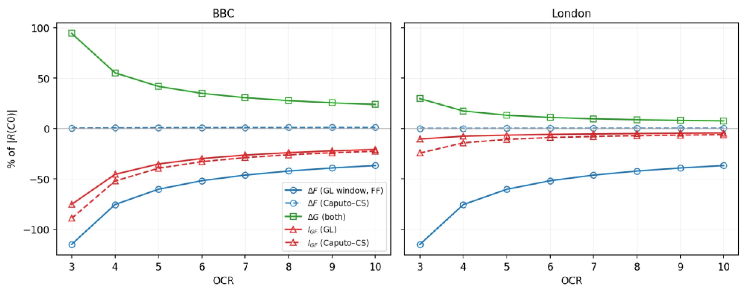
Figure 5.
Where the flow effect lives (OCR = 5): under the GL window it is a main effect; under the critical-state Caputo operator it migrates into the geometry×flow interaction.
Figure 5.
Where the flow effect lives (OCR = 5): under the GL window it is a main effect; under the critical-state Caputo operator it migrates into the geometry×flow interaction.
5. Two Routes to State-Dependent Non-Associativity: A Clean Discriminant
State-dependent non-associativity has classically been introduced through explicit state variables — the state parameter of Been and Jefferies [33], the state-dependent dilatancy of Li and Dafalias [34] and its two-surface and bounding-surface realisations [35,36] — and, in overconsolidated-clay modelling, through interpolation constructions of the MIT type [37]. The program now contains two distinct mechanisms that generate state-dependent non-associated flow on the same surface family without an explicit state variable: the interpolation-exponent route of [22], in which the critical stress ratio is scaled as Mk = M·−n with n tied to overconsolidation, and the critical-state Caputo route [9], in which non-locality toward a fixed critical-state terminal modulates the flow direction. The results above yield a discriminant that is independent of calibration: the Caputo route holds the phase-transformation point fixed at * = e−1/Ψ for every α and every OCR and modulates only the approach to it, whereas the interpolation route moves the phase-transformation point with state. For the Boston Blue Clay shape these anchor points are far apart (0.490 versus 0.341, Figure 1), so undrained effective-stress paths of heavily overconsolidated samples — whose contractive-to-dilative transition is expected, by analogy with the phase-transformation behaviour long resolved experimentally in sands since Ishihara et al. [38] and with the steady/critical state established there as a robust reference [39] — should distinguish the routes directly. A comparably systematic phase-transformation database for heavily overconsolidated clays is sparser, which we flag as a limitation of the proposed discriminant. A quantitative equivalence fit (whether an effective n(OCR) exists that reproduces the Caputo dilatancy within data scatter) is deliberately left to future work, since it must be conducted against laboratory data at the full-model level rather than at the component level isolated here.
6. Limitations
The scope restrictions of the companion study [21] carry over unchanged and are restated rather than resolved: one idealized shear-strain-controlled constant-p′ path with an approximate undrained variant; the α(OCR) form remains an uncalibrated modeling assumption (the collapse results were obtained under the same assumption as the companion for comparability, and were additionally checked at constant α = 0.55 and 0.75, Section 4.1, supporting a structural rather than α-specific mechanism); the compression law retains its calibration-domain idealisation; and the critical-state Caputo flow rule itself has not been validated against laboratory data — the present paper establishes its exact construction, its limits, and its factorial consequences, not its empirical superiority. The log-conjugate convention for the dilatancy magnitude is one of the admissible Jacobian conventions; the location of the zero, the associativity at the critical state, and the collapse results are convention-independent under the stated endpoint, loading, and convergence conditions, but reported magnitudes of D are not.
7. Conclusions
First, the teardrop bounding surface admits an exact critical-state Caputo fractional gradient in closed form once the operator is defined with respect to the log-stress function ψ = ln(1/) [24]: the critical-state terminal is exactly t* = 1/Ψ (* = e−1/Ψ, independent of Ω), and the gradient reduces to incomplete-Beta–Kummer 1F1 (tip terminal) and Humbert Φ1 (critical-state terminal, both sides) expressions, verified against singularity-aware quadrature over 1,240 cases to relative errors below 10−11 (worst case 5.1×10⁻¹² on the far dry side; tip-terminal and shifted-terminal cases below 10−15); the resulting flow rule recovers integer associated flow (in the log-stress conjugate representation) as α → 1 and its flow vector coincides with the associated (purely deviatoric) vector exactly at the critical state for every fractional order, with a sign-changing two-sided zero.
Second, substituting this operator for the fixed-window GL flow collapses the dominant flow main effect of the companion factorial [21] from −60% to below 1% of the baseline response for both soils included in the factorial analysis at every overconsolidation ratio tested, under drained and approximately undrained paths alike, and the collapse persists across a 12-point constant-α grid (both soils; OCR = 3, 5, 10; α = 0.55, 0.75) with |ΔF| ≤ 2.5%, and under the -conjugate flow convention (|ΔF| < 0.1% at OCR = 5), supporting a structural, convention-independent mechanism: under the loading and convergence conditions verified here, an endpoint identity of the hardening law makes the converged response a function of the terminal state only, and the constant-p′ path makes the shared normalized terminal fix the absolute one.
Third, the collapse is a critical-state dwell effect: at small shear budgets the two operators differ strongly (up to +71% of baseline) and the difference decays monotonically as the state reaches and dwells at the shared critical state — identifying the flow main effect of [21] as a critical-state-displacement effect of the window semantics rather than an operator-independent consequence of fractional non-associativity; the reported −60% is not transferable across window semantics.
Fourth, under the critical-state operator the flow effect is strongly geometry-conditional (simple effects +0.7% on the classical surface versus −38.8% on the teardrop for Boston Blue Clay at OCR = 5), appearing in factorial bookkeeping as a dominant geometry×flow interaction; a numerical corollary under the present model assumptions is that the singular exposure of the embedded compression law is itself flow-dependent, London Clay AJOP-compression configurations remaining regular through OCR = 6 under the Caputo flow where their GL counterparts were undefined.
Fifth, the two available routes to state-dependent non-associativity on this surface family are cleanly distinguishable by a calibration-independent discriminant: the interpolation-exponent route of [22] moves the phase-transformation point with state, while the critical-state Caputo route holds it fixed at e−1/Ψ (0.341 versus 0.490 for the Boston Blue Clay shape), making the discriminant experimentally accessible, in principle, on undrained paths of heavily overconsolidated samples [38,39]. All results inherit the reproducibility standard of the companion study: single locked parameter set, no-clamp singularity semantics, self-testing reference implementation, and full scripts as supplementary material.
Supplementary Materials
The following supporting information can be downloaded at the website of this paper posted on Preprints.org. Supplementary S1 (to accompany submission): dcap_engine.py (closed forms, Hölder-aware tables, exact evaluators), phi1_verify.py (1,240-case verification), ff2_run.py (paired factorial driver), the cached dilatancy tables, and ff_canonical.py, inherited from the companion study [21] (its published Supplementary S2). Every number in Table 4 and Table 5, and the data underlying every figure, regenerate from these scripts; Table 2 and Table 3 record the inherited calibration set of [21,22] and are not re-derived here.
Author Contributions
Conceptualisation, N.K. and T.C.; methodology, N.K. and T.C.; software, T.C.; validation, N.K., and T.C. (independent numerical reproduction); formal analysis, N.K.; investigation, T.C.; resources, S.E.-a. and A.K.; data curation, T.C.; writing—original draft preparation, N.K.; writing—review and editing, N.K., A.K., S.E.-a. and S.S.; visualisation, S.S., A.K. and S.E.-a.; supervision, A.K. and S.E.-a.; project administration, N.K.; funding acquisition, N.K. All authors have read and agreed to the published version of the manuscript.
Funding
This research project was financially supported by Mahasarakham University.
Institutional Review Board Statement
Not applicable.
Informed Consent Statement
Not applicable.
Data Availability Statement
The original contributions presented in this study are included in the article and its Supplementary Materials (closed-form dilatancy engine, paired-factorial driver, closed-form verification and self-testing reproduction scripts with the cached dilatancy tables of record, Supplementary S1). Further inquiries can be directed to the corresponding author.
Acknowledgments
The authors gratefully acknowledge Mahasarakham University for its support in all aspects of this research.
Conflicts of Interest
The authors declare no conflicts of interest.
References
- Sumelka, W. Fractional viscoplasticity. Mech. Res. Commun. 2014, 56, 31–36. [Google Scholar] [CrossRef]
- Sumelka, W. Application of fractional continuum mechanics to rate independent plasticity. Acta Mech. 2014, 225, 3247–3264. [Google Scholar] [CrossRef]
- Sumelka, W. A note on non-associated Drucker–Prager plastic flow in terms of fractional calculus. J. Theor. Appl. Mech. 2014, 52, 571–574. [Google Scholar]
- Sumelka, W.; Nowak, M. Non-normality and induced plastic anisotropy under fractional plastic flow rule: a numerical study. Int. J. Numer. Anal. Methods Geomech. 2016, 40, 651–675. [Google Scholar] [CrossRef]
- Sun, Y.; Shen, Y. Constitutive model of granular soils using fractional-order plastic-flow rule. Int. J. Geomech. 2017, 17, 04017025. [Google Scholar] [CrossRef]
- Sun, Y.; Xiao, Y. Fractional order plasticity model for granular soils subjected to monotonic triaxial compression. Int. J. Solids Struct. 2017, 118–119, 224–234. [Google Scholar] [CrossRef]
- Sun, Y.; Xiao, Y. Fractional order model for granular soils under drained cyclic loading. Int. J. Numer. Anal. Methods Geomech. 2017, 41, 555–577. [Google Scholar] [CrossRef]
- Sun, Y.; Indraratna, B.; Carter, J.P.; Marchant, T.; Nimbalkar, S. Application of fractional calculus in modelling ballast deformation under cyclic loading. Comput. Geotech. 2017, 82, 16–30. [Google Scholar] [CrossRef]
- Sun, Y.; Gao, Y.; Zhu, Q. Fractional order plasticity modelling of state-dependent behaviour of granular soils without using plastic potential. Int. J. Plast. 2018, 102, 53–69. [Google Scholar] [CrossRef]
- Sun, Y.; Gao, Y.; Chen, C. Critical-state fractional model and its numerical scheme for isotropic granular soil considering state dependence. Int. J. Geomech. 2019, 19, 04019001. [Google Scholar] [CrossRef]
- Sun, Y.; Gao, Y.; Shen, Y. Mathematical aspect of the state-dependent stress–dilatancy of granular soil under triaxial loading. Géotechnique 2019, 69, 158–165. [Google Scholar] [CrossRef]
- Sun, Y.; Gao, Y.; Shen, Y. Non-associative fractional-order bounding-surface model for granular soils considering state dependence. Int. J. Civ. Eng. 2019, 17, 171–179. [Google Scholar] [CrossRef]
- Sun, Y.; Sumelka, W. State-dependent fractional plasticity model for the true triaxial behaviour of granular soil. Arch. Mech. 2019, 71, 23–47. [Google Scholar] [CrossRef]
- Sun, Y.; Sumelka, W. Fractional viscoplastic model for soils under compression. Acta Mech. 2019, 230, 3365–3377. [Google Scholar] [CrossRef]
- Sun, Y.; Sumelka, W. Multiaxial stress-fractional plasticity model for anisotropically overconsolidated clay. Int. J. Mech. Sci. 2021, 205, 106598. [Google Scholar] [CrossRef]
- Szymczyk, M.; Nowak, M.; Sumelka, W. Numerical study of dynamic properties of fractional viscoplasticity model. Symmetry 2018, 10, 282. [Google Scholar] [CrossRef]
- Lu, D.; Liang, J.; Du, X.; Ma, C.; Gao, Z. Fractional elastoplastic constitutive model for soils based on a novel 3D fractional plastic flow rule. Comput. Geotech. 2019, 105, 277–290. [Google Scholar] [CrossRef]
- Qu, P.; Sun, Y.; Sumelka, W. Review on stress-fractional plasticity models. Materials 2022, 15, 7802. [Google Scholar] [CrossRef] [PubMed]
- Roscoe, K.H.; Burland, J.B. On the generalized stress–strain behaviour of ‘wet’ clay. In Engineering Plasticity; Heyman, J., Leckie, F.A., Eds.; Cambridge University Press: Cambridge, UK, 1968; pp. 535–609. [Google Scholar]
- Schofield, A.N.; Wroth, C.P. Critical State Soil Mechanics; McGraw-Hill: London, UK, 1968. [Google Scholar]
- Kaewhanam, N.; Chatwong, T.; Kampala, A.; Eua-apiwatch, S.; Sultornsanee, S. Continuous Geometry, Continuous Flow, Continuous Compression: A Numerical Component-Interaction Assessment for Fractional Clay Plasticity. Fractal Fract. 2026, 10, 501. [Google Scholar] [CrossRef]
- Chatwong, T.; Kaewhanam, N.; Kaewplang, S.; Phonchamni, N.; Inthidech, S.; Kampala, A.; Sultornsanee, S. A robust constitutive model for clays over a wide range of plasticity and overconsolidation ratio (OCR) with symmetric, continuous curvature control of a teardrop yield surface. Symmetry 2026, 18, 215. [Google Scholar] [CrossRef]
- Kaewhanam, N.; Chatwong, T.; Kaewplang, S.; Phonchamni, N.; Kampala, A.; Sultornsanee, S. AJOP-T: A High-Order Hardening Law for Continuous Teardrop Bounding Surface Plasticity. Mathematics 2026. under review (manuscript mathematics-4456356). [Google Scholar] [CrossRef]
- Almeida, R. A Caputo fractional derivative of a function with respect to another function. Commun. Nonlinear Sci. Numer. Simul. 2017, 44, 460–481. [Google Scholar] [CrossRef]
- Fernandez, A.; Fahad, H.M. Weighted fractional calculus: a general class of operators. Fractal Fract. 2022, 6, 208. [Google Scholar] [CrossRef]
- Caputo, M. Linear models of dissipation whose Q is almost frequency independent—II. Geophys. J. R. Astron. Soc. 1967, 13, 529–539. [Google Scholar] [CrossRef]
- Podlubny, I. Fractional Differential Equations; Academic Press: San Diego, CA, USA, 1999. [Google Scholar]
- Samko, S.G.; Kilbas, A.A.; Marichev, O.I. Fractional Integrals and Derivatives: Theory and Applications; Gordon and Breach: Yverdon, Switzerland, 1993. [Google Scholar]
- Gradshteyn, I.S.; Ryzhik, I.M. Table of Integrals, Series, and Products, 8th ed.; Academic Press: Amsterdam, The Netherlands, 2014. [Google Scholar]
- Erdélyi, A.; Magnus, W.; Oberhettinger, F.; Tricomi, F.G. Higher Transcendental Functions, Vol. I; McGraw-Hill: New York, NY, USA, 1953.
- Srivastava, H.M.; Karlsson, P.W. Multiple Gaussian Hypergeometric Series; Ellis Horwood: Chichester, UK, 1985. [Google Scholar]
- Diethelm, K. The Analysis of Fractional Differential Equations; Lecture Notes in Mathematics 2004; Springer: Berlin, Germany, 2010. [Google Scholar] [CrossRef]
- Been, K.; Jefferies, M.G. A state parameter for sands. Géotechnique 1985, 35, 99–112. [Google Scholar] [CrossRef]
- Li, X.S.; Dafalias, Y.F. Dilatancy for cohesionless soils. Géotechnique 2000, 50, 449–460. [Google Scholar] [CrossRef]
- Manzari, M.T.; Dafalias, Y.F. A critical state two-surface plasticity model for sands. Géotechnique 1997, 47, 255–272. [Google Scholar] [CrossRef]
- Dafalias, Y.F. Bounding surface plasticity. I: Mathematical foundation and hypoplasticity. J. Eng. Mech. 1986, 112, 966–987. [Google Scholar] [CrossRef]
- Whittle, A.J.; Kavvadas, M.J. Formulation of MIT-E3 constitutive model for overconsolidated clays. J. Geotech. Eng. 1994, 120, 173–198. [Google Scholar] [CrossRef]
- Ishihara, K.; Tatsuoka, F.; Yasuda, S. Undrained deformation and liquefaction of sand under cyclic stresses. Soils Found. 1975, 15, 29–44. [Google Scholar] [CrossRef]
- Verdugo, R.; Ishihara, K. The steady state of sandy soils. Soils Found. 1996, 36, 81–92. [Google Scholar] [CrossRef] [PubMed]
Figure 1.
Dilatancy structures on the Boston Blue Clay teardrop (Ψ=1.4, Ω=0.93): integer associated flow, critical-state Caputo flow at three fractional orders, and the embedded non-associated rule of [22]. The Caputo family shares the fixed, Ω-independent phase-transformation point = e−1/Ψ = 0.490 with a sign-changing two-sided zero; the embedded rule of [22] crosses at ≈ 0.341. All dilatancies are plotted in M-normalized form (M ≡ 1).
Figure 1.
Dilatancy structures on the Boston Blue Clay teardrop (Ψ=1.4, Ω=0.93): integer associated flow, critical-state Caputo flow at three fractional orders, and the embedded non-associated rule of [22]. The Caputo family shares the fixed, Ω-independent phase-transformation point = e−1/Ψ = 0.490 with a sign-changing two-sided zero; the embedded rule of [22] crosses at ≈ 0.341. All dilatancies are plotted in M-normalized form (M ≡ 1).
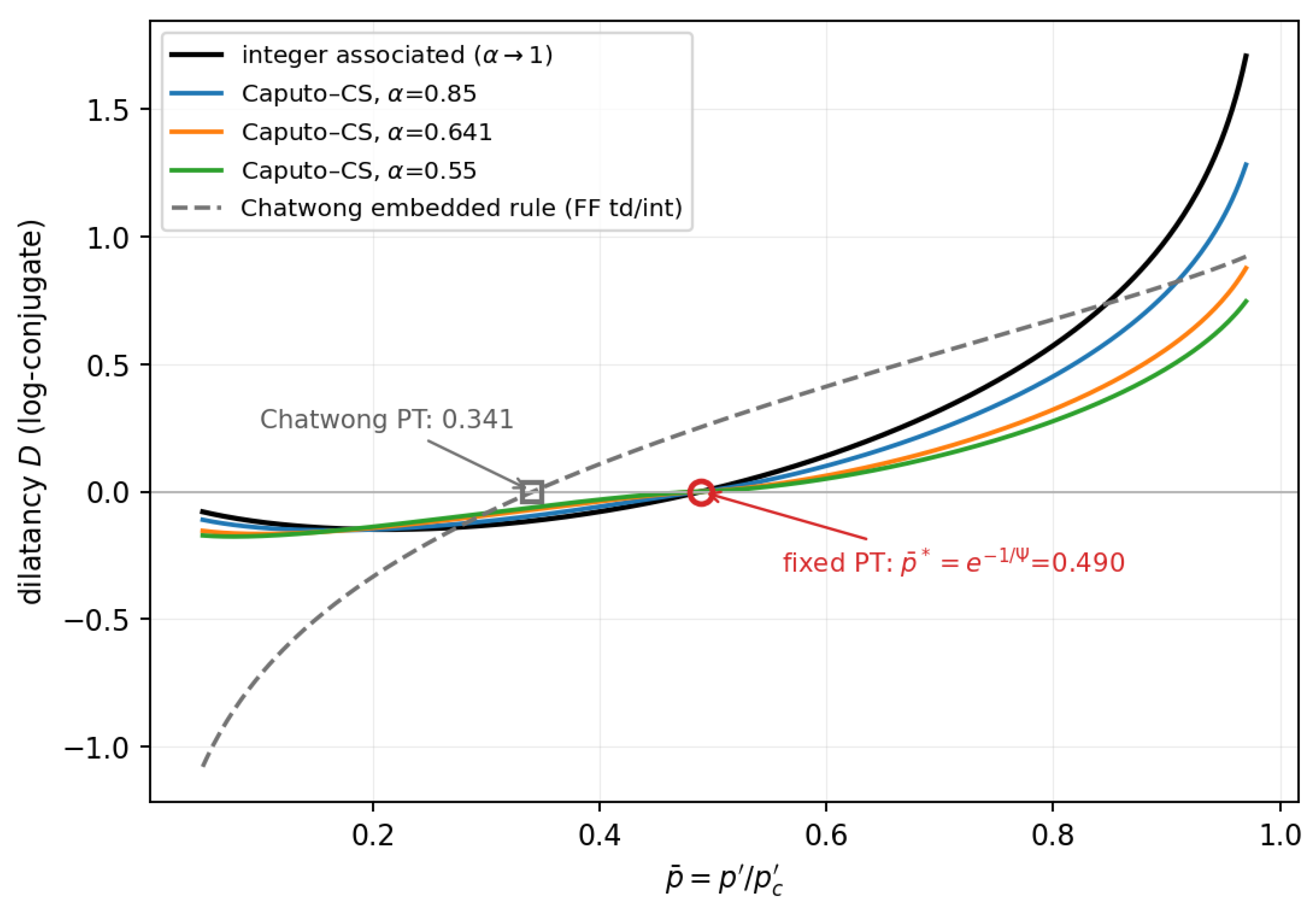
Figure 3.
Decay of the Caputo-CS flow main effect with imposed shear budget (OCR = 5): the effect is a transient of the approach to critical state and vanishes during the critical-state dwell.
Figure 3.
Decay of the Caputo-CS flow main effect with imposed shear budget (OCR = 5): the effect is a transient of the approach to critical state and vanishes during the critical-state dwell.
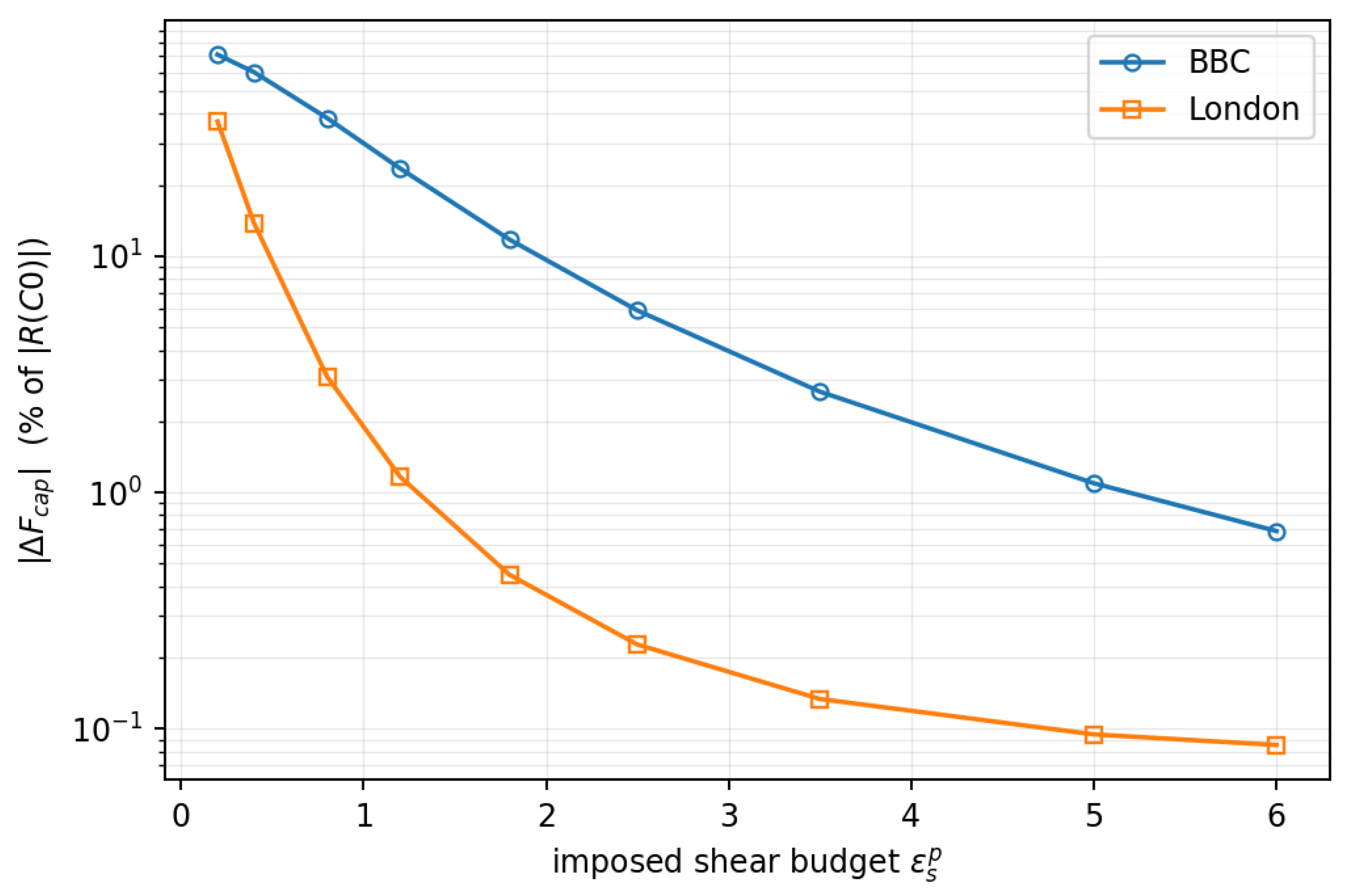
Table 4.
Paired factorial at OCR = 5 (% of |R(C0)|): GL-window pairing (companion) versus critical-state Caputo pairing.
Table 4.
Paired factorial at OCR = 5 (% of |R(C0)|): GL-window pairing (companion) versus critical-state Caputo pairing.
| index | BBC (GL) | BBC (Caputo) | London (GL) | London (Caputo) |
|---|---|---|---|---|
| ΔG | +41.71 | +41.71 | +13.10 | +13.10 |
| ΔF | -60.25 | +0.69 | -60.32 | +0.10 |
| ΔC | +21.38 | +21.38 | +37.97 | +37.97 |
| IGF | -35.21 | -39.46 | -6.59 | -10.80 |
| IGC | -17.58 | -17.58 | -10.30 | -10.30 |
| IFC | +41.70 | -0.60 | undef. | +0.13 |
| IGFC | +12.39 | +16.38 | undef. | +8.38 |
Table 5.
Caputo-CS pairing across OCR = 3–10 (% of |R(C0)|). “undef.” marks indices rendered undefined by the hardening singularity (no-clamp semantics).
Table 5.
Caputo-CS pairing across OCR = 3–10 (% of |R(C0)|). “undef.” marks indices rendered undefined by the hardening singularity (no-clamp semantics).
| BBC | |||||||
| OCR | ΔG | ΔF | ΔC | IGF | IGC | IFC | IGFC |
| 3 | +94.24 | +0.28 | +1.19 | -89.06 | -2.04 | -0.13 | +1.17 |
| 4 | +55.13 | +0.51 | +12.89 | -52.13 | -14.12 | -0.40 | +12.96 |
| 5 | +41.71 | +0.69 | +21.38 | -39.46 | -17.58 | -0.60 | +16.38 |
| 6 | +34.79 | +0.81 | +27.81 | -32.92 | -18.81 | -0.74 | +17.62 |
| 7 | +30.51 | +0.89 | +32.88 | -28.89 | -19.19 | -0.82 | +18.03 |
| 8 | +27.58 | +0.94 | +36.98 | -26.11 | -19.20 | -0.87 | +18.07 |
| 9 | +25.42 | +0.96 | +40.38 | -24.07 | -19.04 | -0.89 | +17.94 |
| 10 | +23.76 | +0.98 | +43.26 | -22.50 | -18.80 | -0.90 | +17.73 |
| London | |||||||
| OCR | ΔG | ΔF | ΔC | IGF | IGC | IFC | IGFC |
| 3 | +29.57 | +0.04 | +9.58 | -24.37 | -7.98 | +0.05 | +6.26 |
| 4 | +17.31 | +0.07 | +26.26 | -14.27 | -10.13 | +0.09 | +8.19 |
| 5 | +13.10 | +0.10 | +37.97 | -10.80 | -10.30 | +0.13 | +8.38 |
| 6 | +10.93 | +0.12 | +46.60 | -9.02 | -10.05 | +0.18 | +8.20 |
| 7 | +9.59 | +0.14 | undef. | -7.92 | undef. | undef. | undef. |
| 8 | +8.67 | +0.16 | undef. | -7.16 | undef. | undef. | undef. |
| 9 | +7.99 | +0.17 | undef. | -6.61 | undef. | undef. | undef. |
| 10 | +7.47 | +0.18 | undef. | -6.18 | undef. | undef. | undef. |
Disclaimer/Publisher’s Note: The statements, opinions and data contained in all publications are solely those of the individual author(s) and contributor(s) and not of MDPI and/or the editor(s). MDPI and/or the editor(s) disclaim responsibility for any injury to people or property resulting from any ideas, methods, instructions or products referred to in the content. |
© 2026 by the authors. Licensee MDPI, Basel, Switzerland. This article is an open access article distributed under the terms and conditions of the Creative Commons Attribution (CC BY) license (http://creativecommons.org/licenses/by/4.0/).
Copyright: This open access article is published under a Creative Commons CC BY 4.0 license, which permit the free download, distribution, and reuse, provided that the author and preprint are cited in any reuse.


