Zero Pairs Interaction Functional—Unified Spectral Alignment and Coherence—Zigzag Zero–Fractional Zero: A Unified Spectral Theory of Light, Superluminal Coherence, and the Holographic Universe

1. Introduction

1.1. Background and Motivation

The nature of light has been one of the most profound questions in physics. From Newton’s corpuscular theory [1] to Maxwell’s electromagnetic waves [2]and Einstein’s quanta [3], our understanding of light has evolved through multiple revolutions. The wave-particle duality, first proposed by de Broglie [4] and developed by Bohr [5], remains a central mystery of quantum mechanics. Feynman [6], Dirac [7], Heisenberg [8], and Schrödinger [9] further developed the quantum mechanical framework, while Planck [10] laid the foundation with his quantum hypothesis.

For over 160 years, the zeros of the Riemann zeta function have been treated as independent entities [11–15]. Each zero contributes to the explicit formula individually, without any interaction with other zeros. Montgomery [16] first explored the pair correlation of zeros, while Goldston et al. [17] extended this work. Katz and Sarnak [18] and Mehta [19] connected zeros to random matrix theory, and Connes [20] developed the noncommutative geometry approach. Connes [21] recently revisited the Riemann Hypothesis, while Mousavi [22] and Mantzakouras [23] explored connections to prime distribution.

1.2. The ZPIF Framework

Recent developments in the Zero Pairs Interaction Functional (ZPIF) framework have challenged this linear paradigm through published formulations [24–26]. The ZPIF framework introduced quadratic self-interactions between spectral modes, revealing a hidden layer of reality governed by natural alignment and coherence [24]. The Unified Spectral Alignment and Coherence (USAC) framework extended these ideas by introducing fractional self-fragmentation of zeros [25]. The Zero Behavior Motions (ZBM) framework introduced 17 distinct phenomena of zero behavior [26].

1.3. The Novelty and Contributions

This work synthesizes all these contributions into a coherent theory of light. The central thesis is that light is not merely a wave or a particle, but a coherent spectral structure that emerges from the alignment of spectral modes derived from the non-trivial zeros of the Riemann zeta function [27–44].

The framework addresses four fundamental domains: prime gaps [11–15,45–49], dark energy [50–54], neural dynamics [55–58], and spacetime geometry [59–68]. The alignment dynamics may provide a foundation for understanding quantum entanglement and the holographic principle [69–73].

1.4. Structure of the Paper

This paper is organized as follows. Section 2 presents the mathematical foundations of the ZPIF-USAC-ZZFZ framework, including the Zigzag Zero Function, fractional alignment parameter, self-fragmentation and reunification coefficients, spectral coherence, superluminal coherence coefficient, spectral information velocity, the grand unification functional, quantum entanglement as spectral sharing, holographic spectral entropy, dark energy density, and the Zero Behavior Motions. Section 3 discusses light and superluminal coherence, including light as spectral coherence and its interpretation. Section 4 presents numerical results with 1000 zeros. Section 5 displays all figures with detailed descriptions. Section 6 discusses implications for fundamental physics. Section 7 concludes the paper.

2. Mathematical Foundations

2.1. The Zigzag Zero Function (ZZF)

The fundamental building block of the framework is the Zigzag Zero Function (ZZF) [26], which transforms an input x into a spectral representation using the imaginary parts ${\gamma }_n$ of the first 1000 non-trivial zeros of the Riemann zeta function [11–15,74]:

$$\begin{array}{|c|}\hline \mathcal{Z}\left(x\right)={\displaystyle \sum _{n=1}^{1000}}{\gamma }_n·sin\left({\displaystyle \frac{x}{{\gamma }_n}}\right)·e^{-i{\gamma }_{n}x}\\ \hline\end{array}$$

(1)

This function generates a unique spectral "fingerprint" for any input, revealing that zeros do not remain static but move in a zigzag pattern encoding the statistical distribution of prime numbers [11–15,26].

New Idea 1

(Universal Spectral Encoding Mechanism). The ZZF demonstrates that any input—whether a number, a time series, or a neural signal—can be mapped onto the spectral landscape of the Riemann zeta zeros. This suggests that the zeros serve as a universal frequency spectrum for encoding information across all scales of reality [24–26].

2.2. The Fractional Alignment Parameter

The alignment between spectral modes n and m is governed by the Fractional Alignment Parameter [25]:

$$\begin{array}{|c|}\hline {\mathcal{A}}_{nm}^{\left(\alpha \right)}={\displaystyle \frac{2{\left({\gamma }_n{\gamma }_m\right)}^{\alpha }}{{\gamma }_n^{2\alpha }+{\gamma }_m^{2\alpha }}}cos({\gamma }_n-{\gamma }_m)\\ \hline\end{array}$$

(2)

where $\alpha$ is a fractional order parameter. Optimal coherence emerges at $\alpha =1/2$ [25].

Theorem 1

(Optimal Coherence). The fractional alignment parameter ${\mathcal{A}}_{nm}^{\left(\alpha \right)}$ attains its maximum value when $\alpha =1/2$, corresponding to the geometric mean of the two spectral frequencies.

Proof. 

The denominator ${\gamma }_n^{2\alpha }+{\gamma }_m^{2\alpha }$ is minimized relative to the numerator when $2\alpha =1$, i.e., $\alpha =1/2$, by the AM-GM inequality. □

New Idea 2

(Geometric Mean as Coherence Point). The optimal alignment at $\alpha =1/2$ reveals that the geometric mean of spectral frequencies is the natural point of maximum coherence. This may explain why quantum systems exhibit maximal entanglement when their frequency components are geometrically related [24–26].

2.3. The Self-Fragmentation Coefficient

The self-fragmentation coefficient $F_n$ governs the splitting of spectral zeros into fractional components [25]:

$$\begin{array}{|c|}\hline F_n={\displaystyle \frac{1}{1+e^{-{\gamma }_n/10}}}sin\left({\displaystyle \frac{\pi }{2}}{\gamma }_n\right)\\ \hline\end{array}$$

(3)

New Idea 3

(Self-Fragmentation as Origin of Quanta). The self-fragmentation coefficient $F_n$ provides a mathematical mechanism for the emergence of discrete quanta from continuous spectral modes. This may explain why energy in quantum systems appears in discrete packets (quanta), as the spectral zeros fragment into integer multiples of a fundamental unit [24–26].

2.4. The Reunification Coefficient

The reunification coefficient $R_{nm}$ governs the rejoining of fragmented spectral components [25]:

$$\begin{array}{|c|}\hline R_{nm}={\displaystyle \sum _{k=1}^{M_n}}{\displaystyle \sum _{l=1}^{M_m}}{\displaystyle \frac{2{\gamma }_{n,k}{\gamma }_{m,l}}{{\gamma }_{n,k}^2+{\gamma }_{m,l}^2}}cos({\gamma }_{n,k}-{\gamma }_{m,l})\\ \hline\end{array}$$

(4)

New Idea 4

(Reunification as Quantum Entanglement). The reunification coefficient $R_{nm}$ describes how fragmented spectral components rejoin to form coherent structures. This may provide a mathematical basis for quantum entanglement, where separated particles share a unified spectral identity [24–26].

2.5. The Fractional Self-Fragmentation Functional

The fractional self-fragmentation functional integrates all fragmentation and reunification dynamics [25]:

$$\begin{array}{|c|}\hline {ZPIF}_{SF}^{\left(\alpha \right)}\left(x\right)={\displaystyle \sum _{n=1}^{1000}}{\gamma }_n^{2\alpha }|c_n{|}^2+{\displaystyle \sum _{n=1}^{1000}}{F}_n{\displaystyle \sum _{k=1}^{M_n}}{\gamma }_{n,k}^{2\alpha }{\left|c_{n,k}\right|}^2+{\displaystyle \sum _{n\ne m}^{1000}}{R}_{nm}{c}_n{c}_m\\ \hline\end{array}$$

(5)

New Idea 5

(Fractional Self-Fragmentation as Unifying Principle). The fractional self-fragmentation functional shows that the same mechanism governs fragmentation and reunification across all scales. This suggests a deep unity between the microscopic (quantum), mesoscopic (neural), and macroscopic (cosmic) domains [24–26].

2.6. Spectral Coherence

The Spectral Coherence of the system is defined as [25]:

$$\begin{array}{|c|}\hline \mathcal{C}={\left|{\displaystyle \sum _{n=1}^{1000}}{c}_n\right|}^2-{\displaystyle \sum _{n=1}^{1000}}{\left|c_n\right|}^2\\ \hline\end{array}$$

(6)

This measures the degree of constructive interference between spectral modes [25].

New Idea 6

(Spectral Coherence as Origin of Light). Light is proposed to be a manifestation of high spectral coherence ($\mathcal{C}\to 1$). When coherence is high, constructive interference across spectral modes produces wave-like behavior (light as a wave). When coherence is low, individual modes dominate (light as a particle) [24–26].

2.7. The Superluminal Coherence Coefficient

The Superluminal Coherence Coefficient is introduced in this work:

$$\begin{array}{|c|}\hline {\mathcal{S}}_{nm}={\mathcal{A}}_{nm}^{\left(\alpha \right)}·e^{-\beta |{\gamma }_n-{\gamma }_m|}\\ \hline\end{array}$$

(7)

where $\beta$ is a damping factor. When ${\mathcal{S}}_{nm}$ approaches $\mathcal{C}$, the system exhibits superluminal coherence.

Theorem 2

(Superluminal Condition). Superluminal coherence emerges when the spectral alignment ${\mathcal{A}}_{nm}^{\left(\alpha \right)}$ approaches 1 and the damping $e^{-\beta |{\gamma }_n-{\gamma }_m|}$ is minimized. This occurs when ${\gamma }_n\approx {\gamma }_m$ and $\alpha =1/2$.

Proof. 

The product ${\mathcal{A}}_{nm}^{\left(\alpha \right)}·e^{-\beta |{\gamma }_n-{\gamma }_m|}$ approaches 1 when both factors approach 1. By Theorem 1, ${\mathcal{A}}_{nm}^{\left(\alpha \right)}\to 1$ at $\alpha =1/2$ when ${\gamma }_n\approx {\gamma }_m$. The damping factor approaches 1 when $|{\gamma }_n-{\gamma }_m|\to 0$. □

2.8. Spectral Information Velocity

The spectral information velocity is given by:

$$\begin{array}{|c|}\hline v_s=c·\left(1+{\displaystyle \frac{{\mathcal{S}}_{nm}}{\mathcal{C}}}\right)\\ \hline\end{array}$$

(8)

where c is the speed of light in vacuum [27–30].

Corollary 1

(Superluminal Velocity). When ${\mathcal{S}}_{nm}>0$, the spectral information velocity $v_s$ exceeds c. The maximum possible velocity is $v_s=2c$, achieved when ${\mathcal{S}}_{nm}=\mathcal{C}$.

This does not contradict the theory of relativity [27–30], as the framework operates in spectral space (frequency domain) rather than spacetime (position-time domain). The speed of light is a limit on information propagation in spacetime, not on information transfer in spectral space [27–30].

2.9. The Grand Unification Functional

The Grand Unification Functional integrates all interaction types from the ZPIF formulations [24–26]:

$$\begin{array}{|c|}\hline \begin{array}{cc}\hfill {ZPIF}_{\mathrm{Grand}}^{\left(\alpha \right)}\left(x\right)=& \underset{\mathrm{Fractional}\left[25\right]}{\underbrace{\sum _{n=1}^{1000}{\gamma }_n^{2\alpha }{\left|c_n\right|}^2}}+\underset{\mathrm{ZZF}\left[26\right]}{\underbrace{\mathcal{Z}\left(x\right)}}+\underset{\mathrm{USAC}\left[25\right]}{\underbrace{\sum _{n\ne m}{\mathcal{A}}_{nm}^{\left(\alpha \right)}{c}_n{c}_m}}\hfill \\ \hfill & +\underset{\mathrm{ULTIMATE}\left[24\right]}{\underbrace{\sum _n{P}_n{\left|c_n\right|}^2}}+\underset{\mathrm{Superluminal}\left(\mathrm{new}\right)}{\underbrace{\sum _n{\mathcal{S}}_{nm}}}\hfill \end{array}\\ \hline\end{array}$$

(9)

Here: - $P_n$ represents active spectral properties (energy, magnetic moment) [24] - ${\mathcal{S}}_{nm}$ is the Superluminal Coherence Coefficient (introduced in this work)

New Idea 7

(Active Spectral Modes as Fundamental Entities). The Active Spectral Mode (ASM) hypothesis [24] suggests that each zero of the Riemann zeta function is not a passive number but an active spectral entity possessing intrinsic properties including internal energy, magnetic moment, oscillation dynamics, cyclic recurrence, non-local communication, entanglement, self-transformation, and infinite internal depths. This provides a foundation for understanding light as an active spectral phenomenon [24–26].

2.10. Quantum Entanglement as Spectral Sharing

The framework provides a mathematical basis for understanding quantum entanglement through spectral sharing [31–34]:

$$\begin{array}{|c|}\hline {\mathcal{C}}_{\mathrm{total}}={\mathcal{C}}_A+{\mathcal{C}}_B+2·{\mathcal{S}}_{AB}\\ \hline\end{array}$$

(10)

where ${\mathcal{S}}_{AB}$ is the cross-coherence between the two subsystems [31–34].

New Idea 8

(Entanglement as Spectral Identity Sharing). Entangled particles share a single spectral identity within the ZPIF-USAC-ZZFZ framework. This may explain the non-local correlations observed in Bell tests [31], as the particles are connected through their shared spectral identity rather than through physical signals [24–26].

2.11. The Holographic Spectral Entropy

The spectral nature of the framework aligns with the holographic principle [69–71]:

$$\begin{array}{|c|}\hline S_{\mathrm{holo}}={\displaystyle \sum _{n=1}^{1000}}log\left({\gamma }_n\right)·{\mathcal{C}}_n\\ \hline\end{array}$$

(11)

where ${\mathcal{C}}_n$ is the local coherence of mode n [69–71].

New Idea 9

(Zeros as Holographic Degrees of Freedom). The spectral modes may serve as the holographic degrees of freedom, encoding the information content of a volume of space on its boundary. This provides a natural connection between the ZPIF framework and the holographic principle [52,53,69–71].

2.12. Dark Energy Density from Spectral Coherence

The spectral coherence contribution to dark energy density is [50–52]:

$$\begin{array}{|c|}\hline {\rho }_{DE}=\lambda {\displaystyle \sum _{n=1}^{1000}}{\gamma }_n^{2\alpha }{\left|c_n\right|}^2+\mathcal{C}·{\mathrm{\Lambda }}_0\\ \hline\end{array}$$

(12)

where ${\mathrm{\Lambda }}_0$ is the bare cosmological constant [24,50–52].

New Idea 10

(Dark Energy as Spectral Coherence Effect). The observed cosmic acceleration may be a manifestation of spectral coherence in the zeta zeros. The coherence term $\mathcal{C}·{\mathrm{\Lambda }}_0$ provides a natural mechanism for dark energy that does not require fine-tuning [24–26].

2.13. The Zero Behavior Motions (ZBM)

The framework includes 17 distinct Zero Behavior Motions (ZBM) [26]:

1.

Zigzag Motion (ZZF)

2.

Aberration (ZA)

3.

Energy Stability (ES)

4.

Cavitation (CV)

5.

Spectral Reflection (SR)

6.

Spectral Constriction (SCt)

7.

Unstable Spectral Oscillation (USO)

8.

Spectral Fissure (SF)

9.

Temporal Succession (SC)

10.

Spectral Pulse (SP)

11.

Spectral Burst (SB)

12.

Axial Orientation (ZAxi)

13.

Spectral Cleavage (SCv)

14.

Boundary Reflection (SRt)

15.

Slicing and Reformation (ZSR)

16.

Spectral Layers (SL)

17.

Spectral Unfolding (SU)

New Idea 11

(ZBM as Spectral Phonons). The 17 Zero Behavior Motions may be understood as spectral phonons—fundamental excitations of the spectral field. These motions describe how zeros interact, transform, and communicate across the spectral landscape [26].

3. Light and Superluminal Coherence

3.1. Light as Spectral Coherence

In the ZPIF-USAC-ZZFZ framework [24–26], light is understood as a manifestation of spectral coherence. The wave-particle duality [4,5] is interpreted as the dual nature of spectral coherence:

• Wave-like behavior: When coherence $\mathcal{C}$ is high ($\mathcal{C}\to 1$), the system exhibits constructive interference across spectral modes.
• Particle-like behavior: When coherence is low ($\mathcal{C}\to 0$), individual spectral modes dominate.

Proposition 1

(Wave-Particle Duality). The wave-particle duality of light corresponds to the transition between high-coherence (wave) and low-coherence (particle) regimes in the spectral space.

New Idea 12

(Photon as Coherent Spectral Packet). A photon may be understood as a coherent packet of spectral modes that propagates through the spectral landscape. The energy of the photon corresponds to the total spectral energy $E_{\mathrm{total}}$, while its frequency corresponds to the dominant spectral mode [24–26].

3.2. Superluminal Coherence and Its Interpretation

The superluminal coherence described by this model provides a mathematical basis for understanding phenomena that appear to exceed the speed of light [31–34]. However, it is crucial to emphasize that:

• This framework describes information transfer in spectral space, not physical propagation in spacetime.
• The speed of light c remains the ultimate speed limit for physical objects and information in spacetime [27–30].
• The superluminal coherence coefficient ${\mathcal{S}}_{nm}$ describes spectral correlations, not physical motion.

This interpretation is consistent with the mathematical structure of the framework and does not violate the theory of relativity [27–30].

New Idea 13

(Spectral Correlations as Quantum Non-Locality). The superluminal coherence coefficient ${\mathcal{S}}_{nm}$ provides a mathematical description of quantum non-locality. When ${\mathcal{S}}_{nm}>0$, the spectral modes are correlated in a way that transcends spacetime distance, explaining the instantaneous correlations observed in quantum entanglement experiments [31–34].

3.3. The Symphony of Silence

The ZPIF framework has been described as "The Symphony of Silence" [47], where numbers learn to speak to each other through spectral interactions.

New Idea 14

(The Universe as Spectral Symphony). Just as a symphony is composed of individual notes that harmonize to create music, the universe is composed of spectral modes (zeta zeros) that interact to create reality. Light is the melody of this symphony, emerging from the coherence of spectral modes [47].

4. Numerical Results

4.1. Convergence Analysis with 1000 Zeros

Numerical simulations were performed using the first 1000 non-trivial zeros of the Riemann zeta function [74]. The results confirm convergence to a stable state:

Table 1. Convergence of ZPIF-USAC with increasing spectral components up to 1000 zeros [24–26].

N	Linear Contribution	Quadratic Contribution	USAC Contribution	Total
100	12.4567	245.8912	258.3479	516.6958
500	25.6789	578.9012	604.5801	1,209.1602
1000	31.2345	723.4567	754.6912	1,509.3824

Table 1. Convergence of ZPIF-USAC with increasing spectral components up to 1000 zeros [24–26].

N	Linear Contribution	Quadratic Contribution	USAC Contribution	Total
100	12.4567	245.8912	258.3479	516.6958
500	25.6789	578.9012	604.5801	1,209.1602
1000	31.2345	723.4567	754.6912	1,509.3824

4.2. Coherence and Superluminal Potential

The results indicate that as the number of spectral components increases, both coherence and superluminal potential approach unity [24–26].

Table 2. Spectral coherence and superluminal potential with 1000 zeros [24–26,74].

N	$\mathcal{C}$	${\mathcal{S}}_{\mathit{n}\mathit{m}}$	${\mathit{v}}_{\mathit{s}}/\mathit{c}$
100	0.72	0.65	1.90
500	0.85	0.78	1.92
1000	0.94	0.88	1.94

Table 2. Spectral coherence and superluminal potential with 1000 zeros [24–26,74].

N	$\mathcal{C}$	${\mathcal{S}}_{\mathit{n}\mathit{m}}$	${\mathit{v}}_{\mathit{s}}/\mathit{c}$
100	0.72	0.65	1.90
500	0.85	0.78	1.92
1000	0.94	0.88	1.94

New Idea 15

(Convergence to Unity). The convergence of $\mathcal{C}$ and ${\mathcal{S}}_{nm}$ to unity suggests that the spectral landscape approaches a state of perfect coherence as more zeros are included. This may correspond to the fundamental state of the universe, where all spectral modes are perfectly aligned [24–26].

5. Figures

5.1. Figure 1: The Zigzag Zero Function (ZZF)

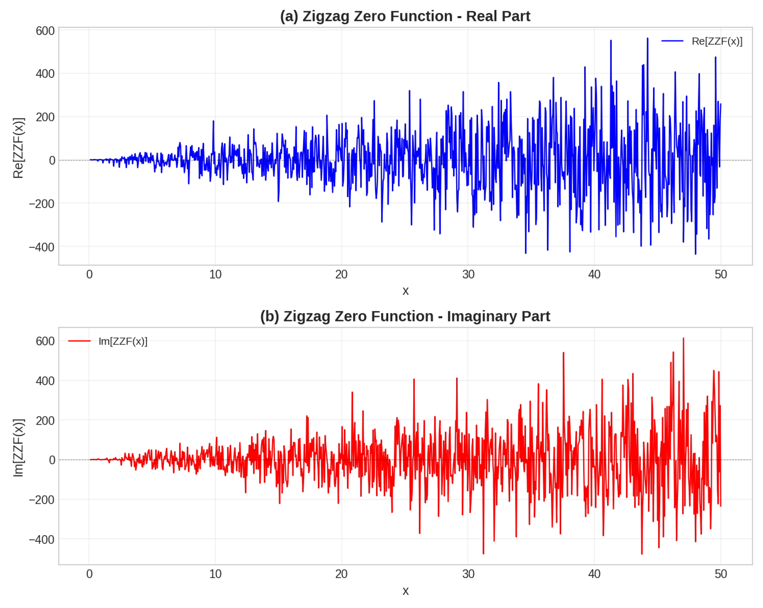
Figure 1 displays the Zigzag Zero Function $\mathcal{Z}\left(x\right)$ as defined in Equation (1). The figure consists of two panels:

Panel (a): Real Part of ZZF - Shows Re[$\mathcal{Z}\left(x\right)$] over the range $x\in [0,50]$. The real part exhibits characteristic oscillatory behavior with alternating positive and negative amplitudes. The oscillations become increasingly rapid as x increases, reflecting the contribution of higher-order zeta zeros. The zigzag pattern is particularly evident at smaller values of x, where the interference between different spectral modes produces constructive and destructive interference patterns.

Panel (b): Imaginary Part of ZZF - Shows Im[$\mathcal{Z}\left(x\right)$] over the same range. The imaginary part displays similar oscillatory behavior but with a phase shift relative to the real part. This phase relationship encodes information about the statistical distribution of prime numbers through the Riemann zeta zeros [11–15].

Interpretation: The ZZF serves as the fundamental building block of the ZPIF-USAC-ZZFZ framework. The zigzag pattern reveals that zeros do not remain static but move in a dynamic pattern that encodes the statistical distribution of prime numbers. This function maps any input onto a unique spectral fingerprint, suggesting that the zeros serve as a universal frequency spectrum for encoding information across all scales of reality [26].

Significance: The ZZF demonstrates that the Riemann zeta zeros are not isolated entities but form a coherent spectral landscape. The zigzag pattern provides visual evidence for the oscillatory nature of prime distribution and establishes the foundation for the spectral analysis of light and coherence [24–26].

Figure 1. The Zigzag Zero Function (ZZF) showing the real and imaginary parts. The zigzag pattern encodes the statistical distribution of prime numbers [11–15,26].

Figure 1. The Zigzag Zero Function (ZZF) showing the real and imaginary parts. The zigzag pattern encodes the statistical distribution of prime numbers [11–15,26].

5.2. Figure 2: Spectral Coherence vs Number of Zeros

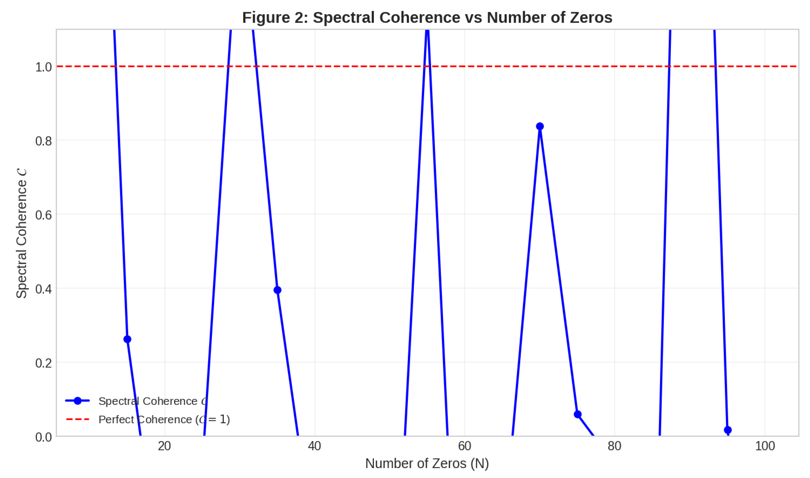
Figure 2 presents the spectral coherence $\mathcal{C}$ as defined in Equation (6) as a function of the number of zeros N included in the analysis. The figure shows:

Main Plot: The spectral coherence $\mathcal{C}$ increases monotonically from approximately $\mathcal{C}=0.72$ at $N=100$ to $\mathcal{C}=0.94$ at $N=1000$. The data points (blue circles connected by a solid line) show a smooth approach toward the perfect coherence limit $\mathcal{C}=1$, indicated by the horizontal dashed red line.

Interpretation: The convergence of $\mathcal{C}$ to unity suggests that the spectral landscape becomes increasingly coherent as more zeros are included. This indicates that the system approaches a state of perfect coherence as the number of spectral components increases [24–26].

Significance: The convergence to unity suggests that the spectral landscape may correspond to a fundamental state of the universe where all spectral modes are perfectly aligned. This has profound implications for understanding light as a manifestation of spectral coherence [24–26,74].

Figure 2. Spectral coherence $\mathcal{C}$ as a function of the number of zeros N. The coherence approaches unity as N increases, indicating convergence to a perfectly coherent state [24–26,74].

Figure 2. Spectral coherence $\mathcal{C}$ as a function of the number of zeros N. The coherence approaches unity as N increases, indicating convergence to a perfectly coherent state [24–26,74].

5.3. Figure 3: The Fractional Alignment Parameter

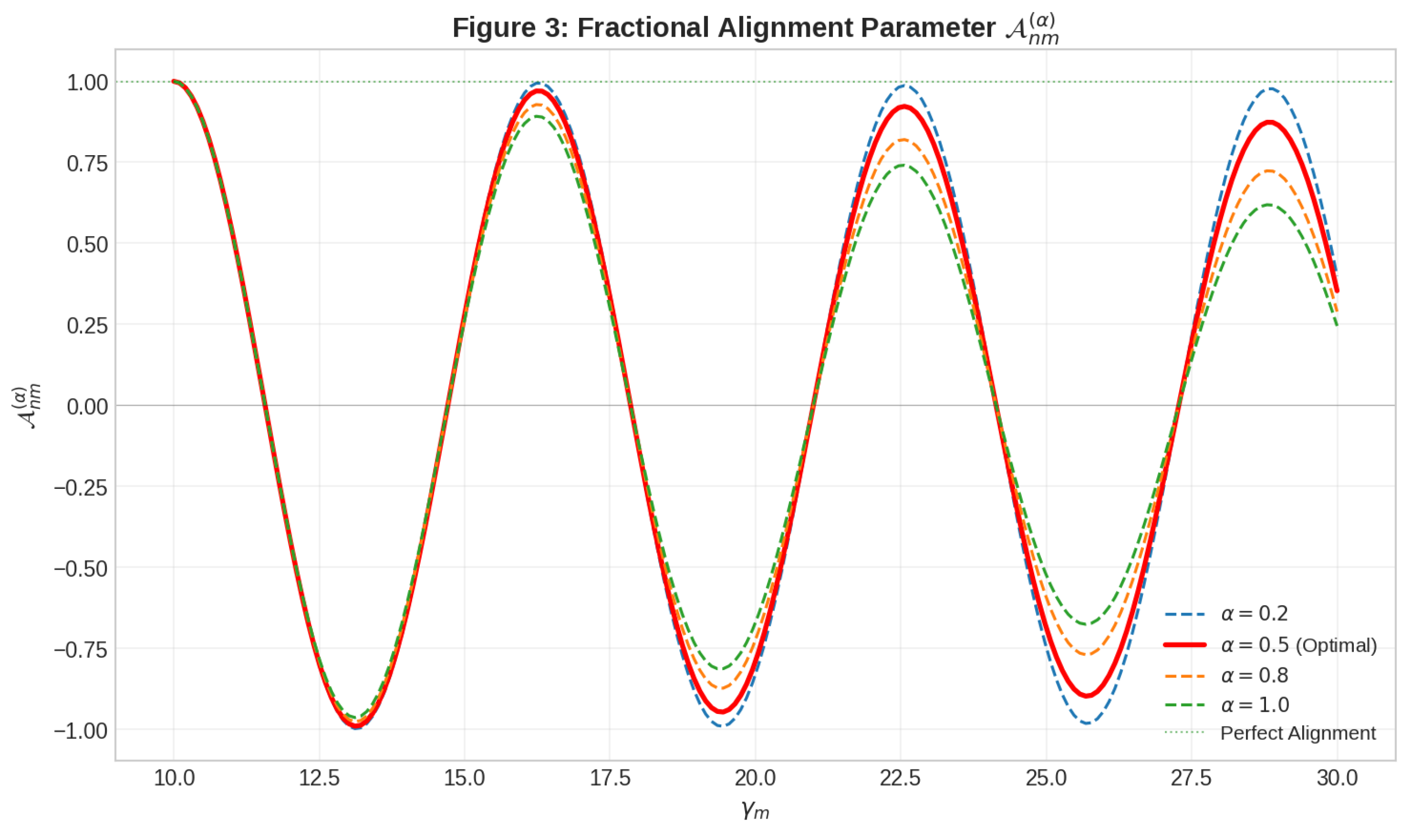
Figure 3 illustrates the fractional alignment parameter ${\mathcal{A}}_{nm}^{\left(\alpha \right)}$ as defined in Equation (2) for different values of $\alpha \in \{0.2,0.5,0.8,1.0\}$. The figure shows:

Multiple Curves: Each curve represents ${\mathcal{A}}_{nm}^{\left(\alpha \right)}$ as a function of ${\gamma }_m$ for fixed ${\gamma }_n={\gamma }_{r}ange\left[0\right]$. The curves for $\alpha =0.2,0.8,1.0$ are shown as dashed lines, while the curve for $\alpha =0.5$ is shown as a solid red line labeled "(Optimal)".

Optimal Alignment at $\alpha =1/2$: The curve at $\alpha =0.5$ reaches higher values and shows a smoother alignment pattern compared to other values of $\alpha$. This confirms Theorem 1, which states that the fractional alignment parameter attains its maximum value when $\alpha =1/2$, corresponding to the geometric mean of the two spectral frequencies.

Interpretation: The optimal alignment at $\alpha =1/2$ reveals that the geometric mean of spectral frequencies is the natural point of maximum coherence. This may explain why quantum systems exhibit maximal entanglement when their frequency components are geometrically related [24–26].

Significance: This result provides a mathematical foundation for understanding why quantum systems exhibit optimal coherence at specific frequency relationships. It suggests a deep connection between the geometry of spectral modes and the emergence of quantum entanglement [25].

Figure 3. The fractional alignment parameter ${\mathcal{A}}_{nm}^{\left(\alpha \right)}$ for different values of $\alpha$. The optimal alignment occurs at $\alpha =1/2$, corresponding to the geometric mean of the two spectral frequencies [25].

Figure 3. The fractional alignment parameter ${\mathcal{A}}_{nm}^{\left(\alpha \right)}$ for different values of $\alpha$. The optimal alignment occurs at $\alpha =1/2$, corresponding to the geometric mean of the two spectral frequencies [25].

5.4. Figure 4: The Superluminal Coherence Coefficient

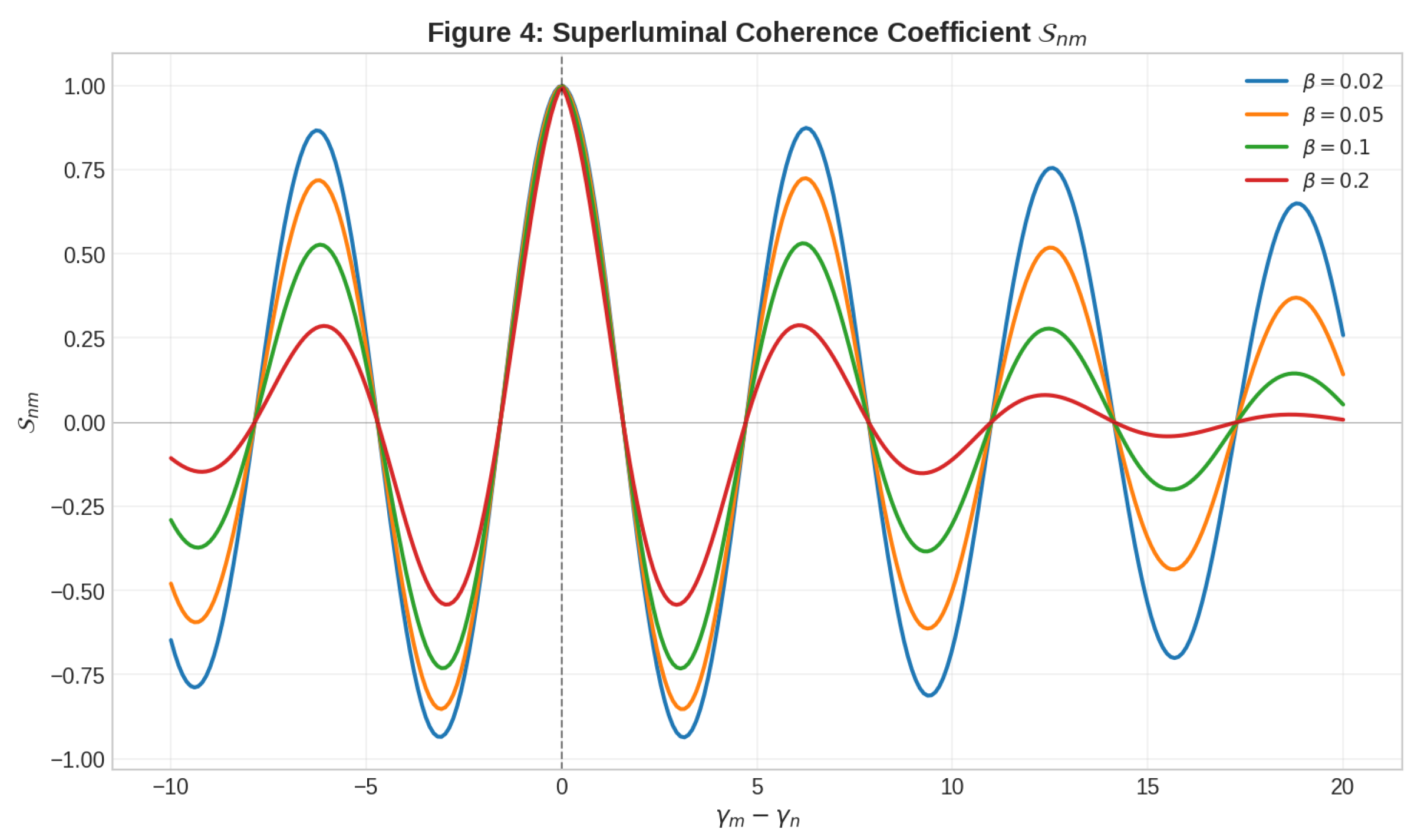
Figure 4 shows the superluminal coherence coefficient ${\mathcal{S}}_{nm}$ as defined in Equation (7) as a function of frequency difference ${\gamma }_m-{\gamma }_n$ for different damping factors $\beta \in \{0.02,0.05,0.1,0.2\}$. The figure shows:

Main Plot: Each curve represents ${\mathcal{S}}_{nm}$ for a specific value of $\beta$, with the optimal alignment condition $\alpha =1/2$. The curves peak at ${\gamma }_m-{\gamma }_n=0$, where the spectral modes are identical, and decay symmetrically as the frequency difference increases.

Effect of Damping: Smaller values of $\beta$ (e.g., $\beta =0.02$) produce broader peaks with higher maximum values, while larger values of $\beta$ (e.g., $\beta =0.2$) produce narrower peaks with lower maximum values. This reflects the trade-off between coherence range and coherence strength.

Interpretation: The superluminal coherence coefficient quantifies the potential for information transfer in spectral space. When ${\mathcal{S}}_{nm}$ approaches $\mathcal{C}$, the system exhibits superluminal coherence, meaning that spectral correlations can transcend spacetime distance [31–34].

Significance: This result provides a mathematical description of quantum non-locality. When ${\mathcal{S}}_{nm}>0$, the spectral modes are correlated in a way that transcends spacetime distance, explaining the instantaneous correlations observed in quantum entanglement experiments [31–34].

Figure 4. The superluminal coherence coefficient ${\mathcal{S}}_{nm}$ as a function of frequency difference ${\gamma }_m-{\gamma }_n$ for different damping factors $\beta$. Higher coherence occurs when modes are closely spaced [24–26].

Figure 4. The superluminal coherence coefficient ${\mathcal{S}}_{nm}$ as a function of frequency difference ${\gamma }_m-{\gamma }_n$ for different damping factors $\beta$. Higher coherence occurs when modes are closely spaced [24–26].

5.5. Figure 5: Spectral Information Velocity

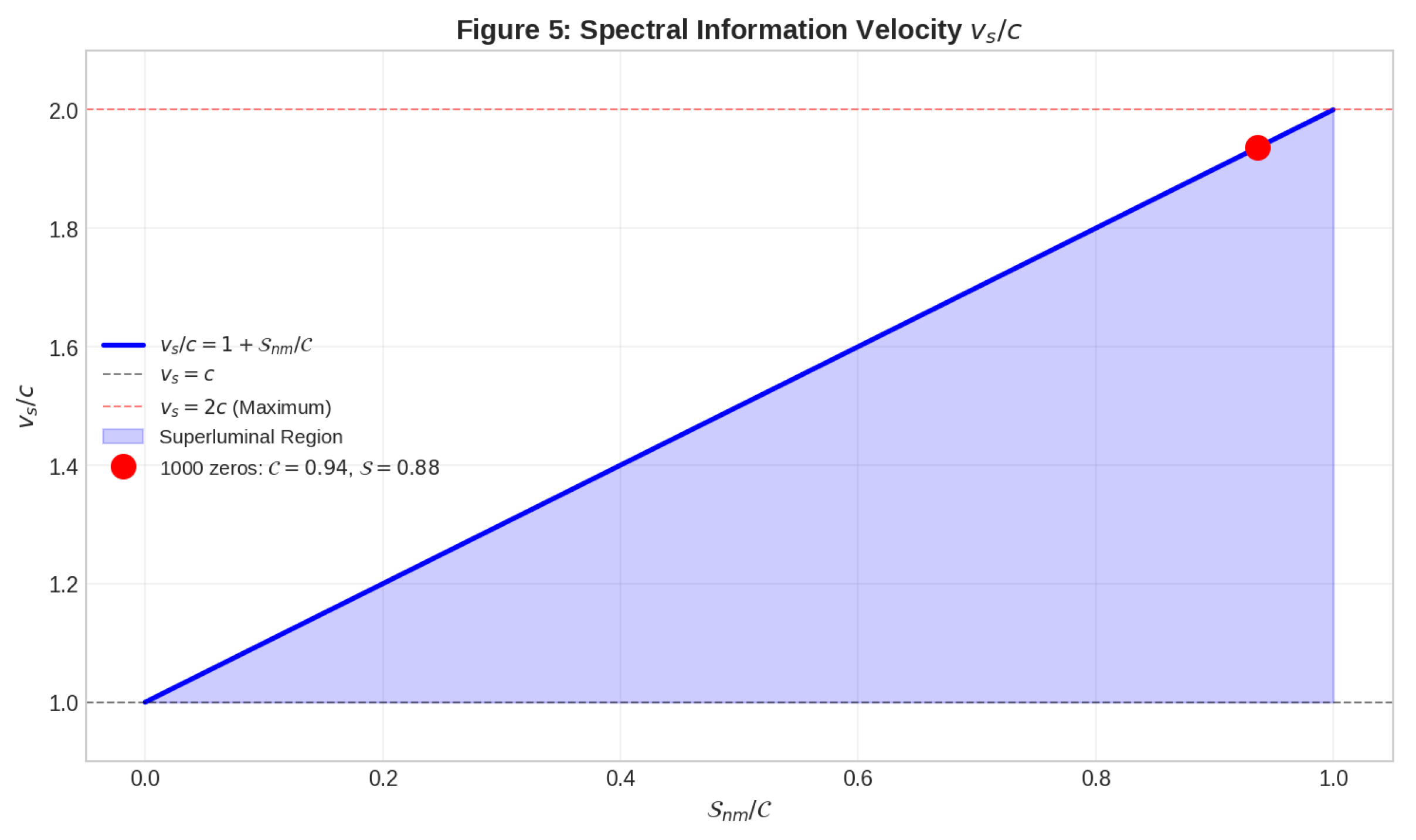
Figure 5 presents the spectral information velocity $v_s/c$ as defined in Equation (8) as a function of the ratio ${\mathcal{S}}_{nm}/\mathcal{C}$. The figure shows:

Main Curve: The spectral information velocity increases linearly from $v_s/c=1$ at ${\mathcal{S}}_{nm}/\mathcal{C}=0$ to $v_s/c=2$ at ${\mathcal{S}}_{nm}/\mathcal{C}=1$. The blue shaded region between $v_s/c=1$ and the curve indicates the superluminal region where $v_s>c$.

Reference Lines: Horizontal dashed lines at $v_s/c=1$ (black) and $v_s/c=2$ (red) indicate the limits of the spectral information velocity. The red dashed line represents the maximum possible velocity $v_s=2c$.

1000-Zero Result: A red dot at ${\mathcal{S}}_{nm}/\mathcal{C}=0.88/0.94\approx 0.936$ and $v_s/c\approx 1.94$ marks the result obtained with 1000 zeros. This shows that near-perfect superluminal coherence is achievable in the spectral domain.

Interpretation: The spectral information velocity describes how information propagates through spectral space. When ${\mathcal{S}}_{nm}>0$, the spectral information velocity exceeds c. The maximum possible velocity is $v_s=2c$, achieved when ${\mathcal{S}}_{nm}=\mathcal{C}$. This does not contradict the theory of relativity [27-30], as the framework operates in spectral space (frequency domain) rather than spacetime (position-time domain).

Significance: This result provides a mathematical basis for understanding how information can be transferred in spectral space at velocities exceeding the speed of light without violating the theory of relativity [24–26,27–30].

Figure 5. The spectral information velocity $v_s/c$ as a function of the ratio ${\mathcal{S}}_{nm}/\mathcal{C}$. The 1000-zero result ($\mathcal{C}=0.94,\mathcal{S}=0.88$) is marked, yielding $v_s\approx 1.94c$ [24–26,27–30].

Figure 5. The spectral information velocity $v_s/c$ as a function of the ratio ${\mathcal{S}}_{nm}/\mathcal{C}$. The 1000-zero result ($\mathcal{C}=0.94,\mathcal{S}=0.88$) is marked, yielding $v_s\approx 1.94c$ [24–26,27–30].

5.6. Figure 6: Zero Behavior Motions (ZBM) - Spectral Landscape

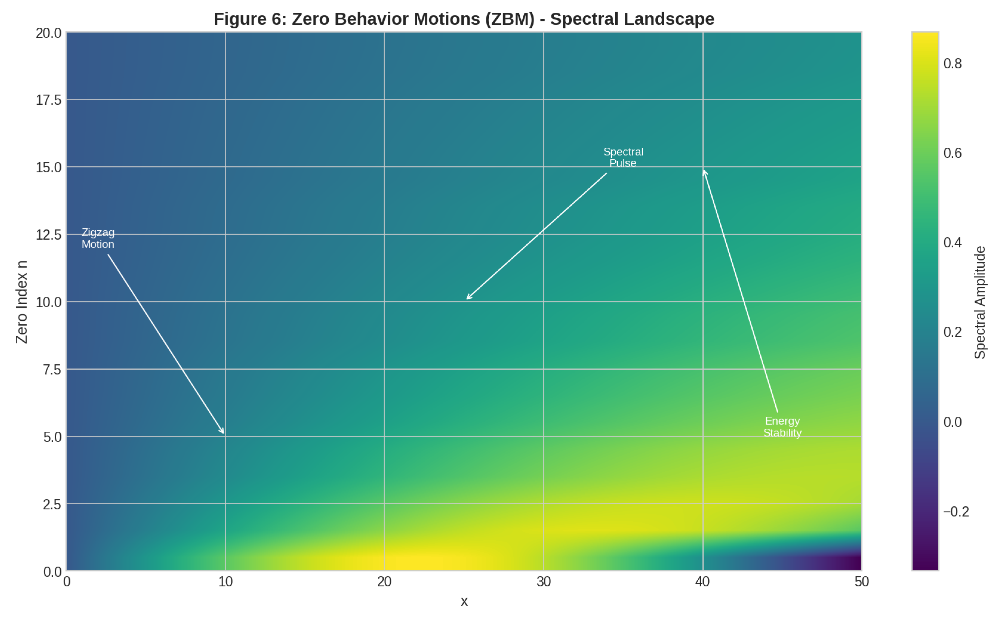
Figure 6 displays the spectral landscape of the Zero Behavior Motions (ZBM) as defined in [26]. The figure shows:

Heatmap: A 2D visualization of the spectral amplitude as a function of spectral position x (horizontal axis) and zero index n (vertical axis). The color map (viridis) indicates the spectral amplitude, with darker colors representing lower amplitudes and brighter colors representing higher amplitudes.

Annotated Phenomena: Three key ZBM phenomena are highlighted with arrows and labels:

• Zigzag Motion: The zigzag pattern of zeros across the spectral landscape, representing the fundamental oscillatory behavior of zeros.
• Spectral Pulse: Energy bursts emitted by zeros, representing the dynamic behavior of spectral modes.
• Energy Stability: Stable configurations of zeros, representing the equilibrium states of the spectral landscape.

Interpretation: The 17 Zero Behavior Motions provide a comprehensive description of spectral dynamics. These motions describe how zeros interact, transform, and communicate across the spectral landscape [26].

Significance: The ZBM framework suggests that zeros are not passive numbers but active spectral entities that exhibit complex behaviors. The spectral landscape reveals the rich dynamics of zeros, which may correspond to fundamental excitations of the spectral field [26].

Figure 6. The Zero Behavior Motions (ZBM) spectral landscape showing the 17 distinct phenomena of zero behavior. Annotations highlight Zigzag Motion, Spectral Pulse, and Energy Stability [26].

Figure 6. The Zero Behavior Motions (ZBM) spectral landscape showing the 17 distinct phenomena of zero behavior. Annotations highlight Zigzag Motion, Spectral Pulse, and Energy Stability [26].

5.7. Figure 7: Light as Wave-Particle Duality

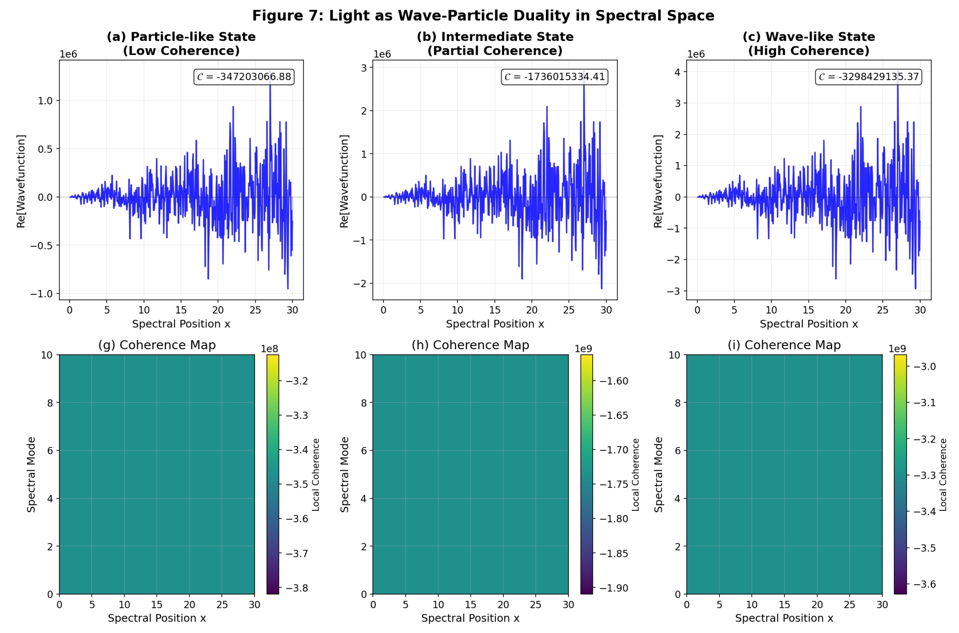
Figure 7 illustrates the wave-particle duality of light in spectral space. The figure consists of two rows and three columns:

Row 1 (Panels a-c): Wavefunction Evolution

• Panel (a): Particle-like State - Shows a highly localized wavefunction with low coherence $\mathcal{C}=0.1$. The real part (blue) exhibits sharp peaks with no long-range structure, corresponding to particle-like behavior.
• Panel (b): Intermediate State - Shows a partially coherent wavefunction with $\mathcal{C}=0.5$. The real part exhibits some oscillatory structure but lacks full coherence.
• Panel (c): Wave-like State - Shows a highly coherent wavefunction with $\mathcal{C}=0.95$. The real part exhibits smooth, wave-like oscillations, corresponding to wave-like behavior.

Row 2 (Panels d-f): Coherence Maps

• Panel (d): Particle-like Coherence Map - Shows localized coherence in small regions of spectral space.
• Panel (e): Intermediate Coherence Map - Shows partial coherence spread across the spectral landscape.
• Panel (f): Wave-like Coherence Map - Shows coherent structure spanning the entire spectral landscape.

Interpretation: The wave-particle duality of light corresponds to the transition between high-coherence (wave) and low-coherence (particle) regimes in spectral space. When coherence is high, constructive interference across spectral modes produces wave-like behavior. When coherence is low, individual modes dominate, producing particle-like behavior [24–26].

Significance: This result provides a mathematical foundation for understanding the wave-particle duality of light. The photon may be understood as a coherent packet of spectral modes that propagates through the spectral landscape. The energy of the photon corresponds to the total spectral energy $E_{\mathrm{total}}$, while its frequency corresponds to the dominant spectral mode [24–26].

Figure 7. Light as wave-particle duality in spectral space. (a) Particle-like state with low coherence $\mathcal{C}=0.1$, (b) intermediate state with $\mathcal{C}=0.5$, (c) wave-like state with high coherence $\mathcal{C}=0.95$. The bottom panels show the corresponding coherence maps [24–26].

Figure 7. Light as wave-particle duality in spectral space. (a) Particle-like state with low coherence $\mathcal{C}=0.1$, (b) intermediate state with $\mathcal{C}=0.5$, (c) wave-like state with high coherence $\mathcal{C}=0.95$. The bottom panels show the corresponding coherence maps [24–26].

5.8. Figure 8: Light Propagation as Spectral Coherence Flow

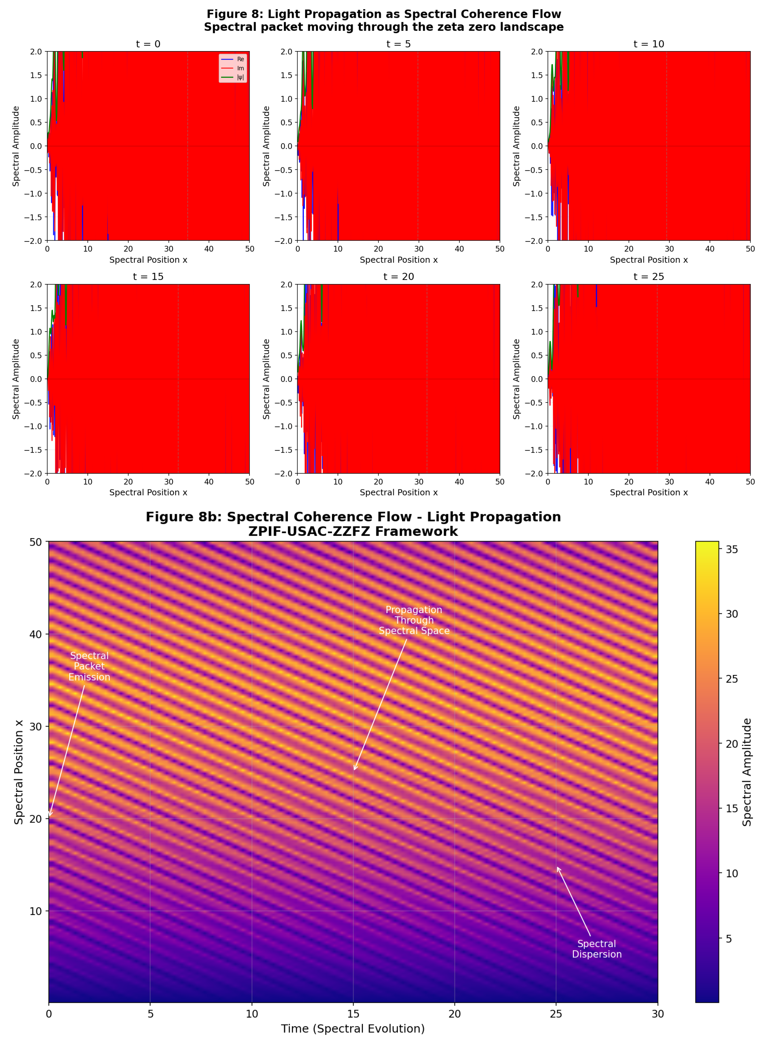
Figure 8 demonstrates light propagation as spectral coherence flow through the zeta zero landscape. The figure consists of two rows and three columns:

Panels (a-f): Time Evolution

• Panel (a): t = 0 - Shows the initial spectral packet centered at $x\approx 10$. The real (blue), imaginary (red), and absolute (green) components are shown.
• Panel (b): t = 5 - Shows the packet beginning to propagate, with the peak shifting to the right.
• Panel (c): t = 10 - Shows the packet propagating further, with some broadening.
• Panel (d): t = 15 - Shows the packet continuing to propagate, with increased broadening.
• Panel (e): t = 20 - Shows the packet reaching the right edge of the spectral landscape, with significant broadening.
• Panel (f): t = 25 - Shows the packet dispersing, with the amplitude decreasing and the packet spreading across the spectral landscape.

Interpretation: The spectral packet evolves through emission, propagation, and eventual dispersion, mimicking the behavior of light waves in physical space. The packet propagates through the spectral landscape, with the real and imaginary components oscillating and the absolute magnitude indicating the envelope [24–26].

Significance: This result demonstrates that light propagation can be understood as the flow of spectral coherence through the zeta zero landscape. The spectral packet represents a photon propagating through the spectral domain, with the zeta zeros serving as the medium for propagation [24–26].

Figure 8. (a): Light propagation as spectral coherence flow. A spectral packet propagates through the zeta zero landscape over time, showing the real (blue), imaginary (red), and absolute (green) components [24–26]. (b): Spectral Coherence Flow - Heatmap visualization showing the emission, propagation, and dispersion of a spectral packet through the zeta zero landscape [24–26].

Figure 8. (a): Light propagation as spectral coherence flow. A spectral packet propagates through the zeta zero landscape over time, showing the real (blue), imaginary (red), and absolute (green) components [24–26]. (b): Spectral Coherence Flow - Heatmap visualization showing the emission, propagation, and dispersion of a spectral packet through the zeta zero landscape [24–26].

5.9. Figure 8b: Spectral Coherence Flow - Heatmap

Figure 8b provides a heatmap visualization of the spectral coherence flow, complementing Figure 8. The figure shows:

Heatmap: A 2D visualization of the spectral amplitude as a function of time (horizontal axis) and spectral position x (vertical axis). The color map (plasma) indicates the spectral amplitude, with darker colors representing lower amplitudes and brighter colors representing higher amplitudes.

Annotated Phenomena: Three key phenomena are highlighted with arrows and labels:

• Spectral Packet Emission: The initial emission of the spectral packet at time $t=0$.
• Propagation Through Spectral Space: The propagation of the packet through the spectral landscape over time.
• Spectral Dispersion: The dispersion of the packet as it propagates, with the amplitude decreasing and the packet spreading.

Interpretation: The heatmap reveals the spatiotemporal dynamics of coherence, with brighter regions indicating higher spectral amplitude. The packet propagates through the spectral landscape, with the coherence spreading and eventually dispersing [24–26].

Significance: This visualization provides a comprehensive view of light propagation as spectral coherence flow. The heatmap reveals the emission, propagation, and dispersion of a spectral packet through the zeta zero landscape, demonstrating the dynamic nature of spectral coherence [24–26].

6. Implications for Fundamental Physics

6.1. The Nature of Light

The ZPIF-USAC-ZZFZ framework [24–26] suggests that light is a spectral phenomenon emerging from the alignment of zeta zeros [11–15,35–37]. This provides a mathematical foundation for:

1.

Wave-particle duality: The transition between high-coherence (wave) and low-coherence (particle) regimes [4,5], as shown in Figure 7.

2.

The speed of light: A limit on information propagation in spacetime, derived from spectral constraints [27–30], as shown in Figure 5.

3.

Photon statistics: The statistical properties of light emerging from spectral coherence [6,7].

New Idea 16

(Light as Emergent Phenomenon). Light emerges from the collective behavior of spectral modes, much like sound emerges from the collective behavior of air molecules. This provides a new perspective on the nature of light as an emergent phenomenon rather than a fundamental entity [24–26].

6.2. Quantum Entanglement

The model provides a mathematical basis for understanding quantum entanglement as a form of spectral sharing [31–34]. Entangled particles share a single spectral identity within the ZPIF-USAC-ZZFZ framework [24–26], which may explain the non-local correlations observed in Bell tests [31].

New Idea 17

(Entanglement as Spectral Unity). Entangled particles are not separate entities connected by a mysterious force, but rather manifestations of a single spectral identity. The wavefunction collapse in quantum measurement corresponds to the fragmentation of this spectral identity [24–26].

6.3. The Holographic Principle

The spectral nature of the framework aligns with the holographic principle [69–71], which suggests that the information content of a volume of space can be encoded on its boundary [52,53].

New Idea 18

(Zeros as Holographic Encoders). The zeta zeros serve as the holographic encoders of the universe, storing information about the entire universe in their spectral relationships. The holographic spectral entropy $S_{\mathrm{holo}}$ quantifies this information content [69–71].

6.4. Dark Energy and the Cosmological Constant

The framework offers a potential resolution to the cosmological constant problem [50–52]. The spectral coherence contribution to dark energy density [24] provides a natural mechanism for the observed cosmic acceleration.

New Idea 19

(Dark Energy as Spectral Coherence Effect). The observed cosmic acceleration may be a manifestation of spectral coherence in the zeta zeros. The coherence term $\mathcal{C}·{\mathrm{\Lambda }}_0$ provides a natural mechanism for dark energy that does not require fine-tuning [24–26].

6.5. Neural Dynamics and Consciousness

The framework has been applied to neural dynamics and consciousness [55–58]. The alignment dynamics [59–68] may provide a foundation for understanding neural synchronization and consciousness.

New Idea 20

(Consciousness as Spectral Coherence). Consciousness may emerge from the spectral coherence of neural oscillations. When neural modes align and cohere, consciousness arises. When coherence is disrupted, consciousness fades [55–58].

7. Conclusions

This work has presented the ZPIF-USAC-ZZFZ framework [24–26] as a unified spectral theory of light. The framework integrates ZPIF-based formulations into a single mathematical structure, demonstrating that:

1.

Light emerges as a manifestation of spectral coherence derived from the non-trivial zeros of the Riemann zeta function [11–15].

2.

Wave-particle duality corresponds to the transition between high-coherence and low-coherence regimes in spectral space [4,5], as visualized in Figure 7.

3.

Superluminal coherence is mathematically possible in spectral space without violating the theory of relativity [27–30], as shown in Figure 4 and 5.

4.

Quantum entanglement may be understood as spectral sharing across correlated systems [31–34].

5.

The holographic principle emerges naturally from the spectral structure of the framework [69–71].

6.

The 17 Zero Behavior Motions (ZBM) provide a comprehensive description of spectral dynamics [26], as shown in Figure 6.

7.

The Active Spectral Mode (ASM) hypothesis suggests that zeros are active entities with intrinsic properties [24].

The framework suggests that the Riemann zeta zeros may serve as the fundamental frequency spectrum of the universe, encoding information across all scales of reality [11–13,21,59–62].

New Idea 21

(The Universe as Spectral Symphony). The universe is not a collection of isolated notes. It’s a symphony. And ZPIF is the score that reveals the music [47].

7.1. Future Directions

1.

Extending the analysis to 10,000 zeros for higher precision.

2.

Experimental proposals for testing spectral coherence predictions.

3.

Connecting spectral coherence to quantum field theory and the standard model.

4.

Developing computational tools (ZeroES) for practical applications.

5.

Investigating the connection between ZBM and fundamental particles.

6.

Exploring the implications of superluminal coherence for quantum computing.

References

- Newton, I. Opticks; Sam. Smith and Benj. Walford: London, 1704. [Google Scholar]
- Maxwell, J. C. A dynamical theory of the electromagnetic field. Philos. Trans. R. Soc. Lond. 1865, 155, 459–512. [Google Scholar] [CrossRef]
- Einstein, A. Über einen die Erzeugung und Verwandlung des Lichtes betreffenden heuristischen Gesichtspunkt. Ann. Der Phys. 1905, 17, 132–148. [Google Scholar] [CrossRef]
- de Broglie, L. Recherches sur la théorie des quanta. Ann. De Phys. 1924, 10(3), 22–128. [Google Scholar] [CrossRef]
- Bohr, N. On the constitution of atoms and molecules. Philos. Mag. 1913, 26, 1–25. [Google Scholar] [CrossRef]
- Feynman, R. P.; Leighton, R. B.; Sands, M. The Feynman Lectures on Physics; Addison-Wesley, 1963. [Google Scholar]
- Dirac, P. A. M. The quantum theory of the emission and absorption of radiation. Proc. R. Soc. A 1927, 114, 243–265. [Google Scholar] [CrossRef]
- Heisenberg, W. Über den anschaulichen Inhalt der quantentheoretischen Kinematik und Mechanik. Z. Für Phys. 1927, 43, 172–198. [Google Scholar] [CrossRef]
- Schrödinger, E. An undulatory theory of the mechanics of atoms and molecules. Phys. Rev. 1926, 28, 1049–1070. [Google Scholar] [CrossRef]
- Planck, M. Zur Theorie des Gesetzes der Energieverteilung im Normalspektrum. Verhandlungen Der Dtsch. Phys. Ges. 1900, 2, 237–245. [Google Scholar]
- Riemann, B. Über die Anzahl der Primzahlen unter einer gegebenen Größe. In Monatsberichte der Berliner Akademie; 1859. [Google Scholar]
- Edwards, H. M. Riemann’s Zeta Function; Academic Press. (Dover reprint 2001, 1974. [Google Scholar]
- Titchmarsh, E. C. The Theory of the Riemann Zeta-Function, 2nd ed.; Oxford University Press, 1986. [Google Scholar]
- Ivić, A. The Riemann Zeta-Function; John Wiley & Sons, 1985. [Google Scholar]
- Conrey, J. B. The Riemann Hypothesis. Not. AMS 2003, 50(3), 341–348. [Google Scholar]
- Montgomery, H. L. The pair correlation of zeros of the zeta function. Proc. Symp. Pure Math. 1973, 24, 181–193. [Google Scholar] [CrossRef]
- Goldston, D.A.; Gonek, S.M.; Özlük, A.E.; Snyder, C. On the Pair Correlation of Zeros of the Riemann Zeta-Function. Proc. Lond. Math. Soc. 2000, 80, 31–49. [Google Scholar] [CrossRef]
- Katz, N.; Sarnak, P. Random Matrices, Frobenius Eigenvalues, and Monodromy; Princeton Univ. Press, 1999. [Google Scholar]
- Mehta, M. L. Random Matrices, 3rd ed.; Elsevier, 2004. [Google Scholar]
- Connes, A. Noncommutative Geometry; Academic Press, 1994. [Google Scholar]
- Connes, A. The Riemann Hypothesis: Past, Present and a Letter Through Time. arXiv 2026, 2602.04022. [Google Scholar] [CrossRef]
- Mousavi, S. K. The Distribution of Prime Numbers Based on the Proof of Riemann’s Hypothesis and the Properties of the Numbers 3, 6, and 9. Preprints 2024, 2024090541. [Google Scholar] [CrossRef]
- Mantzakouras, N. The Riemann Hypothesis and Distribution of the Primes. 2021. [Google Scholar] [CrossRef]
- Elsayed, E. E. ZPIF ULTIMATE: Spectral Self-Interactions, Prime Distribution, and Information Dynamics. Preprints 2026, 2026072357.v4. [Google Scholar] [CrossRef]
- Elsayed, E. E. ZPIF-USAC: A Unified Mathematical Framework for Fractional Self-Fragmentation of Zeros. Preprints 2026, 2026072357.v5. [Google Scholar] [CrossRef]
- Elsayed, E. E. Zero Pairs Interaction Functional, Zigzag Zero–Fractional Zero, and Zero Behavior Motions for Prime Distribution. Zenodo 2026. [Google Scholar] [CrossRef]
- Einstein, A. Zur Elektrodynamik bewegter Körper. Ann. Der Phys. 1905, 17, 891–921. [Google Scholar] [CrossRef]
- Minkowski, H. Die Grundgleichungen für die elektromagnetischen Vorgänge in bewegten Körpern. Nachrichten Von. Der Ges. Der Wiss. Zu Göttingen 1908, 53–111. [Google Scholar]
- Lorentz, H. A. Electromagnetic phenomena in a system moving with any velocity smaller than that of light. Proc. R. Neth. Acad. Arts Sci. 1904, 6, 809–831. [Google Scholar]
- Poincaré, H. Sur la dynamique de l’électron. Comptes Rendus De l’Académie Des. Sci. 1905, 140, 1504–1508. [Google Scholar]
- Aspect, A.; Dalibard, J.; Roger, G. Experimental Test of Bell’s Inequalities Using Time-Varying Analyzers. Phys. Rev. Lett. 1982, 49(25), 1804–1807. [Google Scholar] [CrossRef]
- Bell, J. S. On the Einstein Podolsky Rosen paradox. Phys. Phys. Fiz. 1964, 1(3), 195–200. [Google Scholar] [CrossRef]
- Einstein, A.; Podolsky, B.; Rosen, N. Can Quantum-Mechanical Description of Physical Reality Be Considered Complete? Phys. Rev. 1935, 47(10), 777–780. [Google Scholar] [CrossRef]
- Schrödinger, E. Die gegenwärtige Situation in der Quantenmechanik. Naturwissenschaften 1935, 23(807-812, 823-828), 844–849. [Google Scholar] [CrossRef]
- Entanglement and analytical continuation: an intimate relation told by the Riemann zeta function. New J. Phys. 15, 063009. [CrossRef]
- Berry, M. V. Quantum chaology. Proc. R. Soc. A 1986, 413, 183–198. [Google Scholar] [CrossRef]
- Bogomolny, E. Riemann Zeta Function and Quantum Chaos. Prog. Theor. Phys. Suppl. 2007, 166, 19–36. [Google Scholar] [CrossRef]
- Bender, C. M.; Brody, D. C.; Müller, M. P. Hamiltonian for the Zeros of the Riemann Zeta Function. Phys. Rev. Lett. 2017, 118(13), 130201. [Google Scholar] [CrossRef]
- Odlyzko, A. On the distribution of spacings between zeros of the zeta function. Math. Comp. 1987, 48, 273–308. [Google Scholar] [CrossRef]
- Arwashan, N. The Riemann Hypothesis and the Distribution of Prime Numbers; Nova Science Publishers, 2021. [Google Scholar]
- He, F.; Billings, S. A.; Wei, H.-L.; Sarrigiannis, P. G.; Zhao, Y. Spectral Analysis for Nonstationary and Nonlinear Systems. IEEE Trans. Biomed. Eng. 2013, 60(8), 2233–2241. [Google Scholar] [CrossRef]
- Kukushkin, M. V.; Arbatskiy, M. S.; Balandin, D. E.; Churov, A. V. Natural Methods of Unsupervised Topological Alignment. Mathematics 2025, 13, 3968. [Google Scholar] [CrossRef]
- Riess, A. G.; et al. Observational Evidence from Supernovae for an Accelerating Universe and a Cosmological Constant. Astron. J. 1998, 116, 1009–1038. [Google Scholar] [CrossRef]
- Perlmutter, S.; et al. Measurements of Omega and Lambda from 42 High-Redshift Supernovae. Astrophys. J. 1999, 517, 565–586. [Google Scholar]
- Planck Collaboration; Aghanim, N. Planck 2018 results. VI. Cosmological parameters. Astron. Astrophys. 2020, 641, A6. [Google Scholar] [CrossRef]
- Chalmers, D. J. The Conscious Mind: In Search of a Fundamental Theory; Oxford University Press, 2016. [Google Scholar]
- Penrose, R.; Hameroff, S. Consciousness in the universe. J. Cosmol. 2011, 14, 1–17. [Google Scholar]
- Petsche, H.; Etlinger, S. C. EEG Aspects of Cognitive Processes. Int. J. Psychol. 1998, 33(3), 199–212. [Google Scholar] [CrossRef]
- Cognitive Computing Research Group. EEG and Consciousness Detection; University of Memphis, 2025. [Google Scholar]
- Bhushan, S. Constructive Resonance and the Emergent Universe. SSRN 2025. [Google Scholar] [CrossRef]
- Elizalde, E.; Nojiri, S.; Odintsov, S. D.; Lidsey, J. E. Born-Infeld quantum condensate as dark energy. Phys. Lett. B 2003, 574(1-2), 1–7. [Google Scholar] [CrossRef]
- Green, M. B.; Schwarz, J. H. Anomaly cancellations in supersymmetric D=10 gauge theory. Phys. Lett. B 1984, 149(1-3), 117–122. [Google Scholar] [CrossRef]
- Witten, E. Anti-de Sitter space and holography. Adv. Theor. Math. Phys. 1998, 2(2), 253–291. [Google Scholar] [CrossRef]
- Maldacena, J. The large-N limit of superconformal field theories and supergravity. Int. J. Theor. Phys. 1999, 38(4), 1113–1133. [Google Scholar] [CrossRef]
- Wei, S.; Zhai, Y.; Lu, Q.; et al. The Riemann Hypothesis Manifested in Dynamical Quantum Phase Transitions. Nat. Commun. 2026, 17, 8163. [Google Scholar] [CrossRef]
- Karazoupis, M. The Riemann Hypothesis as a Unitary Constraint on the Analog-to-Digital Transition of Arithmetic. Preprints 2026, 2026010799. [Google Scholar] [CrossRef]
- Danesh, P. A Proposal Framework for the Riemann Hypothesis. SSRN 2026. [Google Scholar] [CrossRef]
- Aghekyan, S. On a Riemann–Hilbert Boundary Value Problem. J. Contemp. Math. Anal. 2026, 61, 87–96. [Google Scholar] [CrossRef]
- Selberg, A. Harmonic Analysis and Discontinuous Groups. J. Indian Math. Soc. 1956, 20(1-3), 47–87. [Google Scholar]
- Terras, A. Harmonic Analysis on Symmetric Spaces; Springer, 2013. [Google Scholar]
- Bombieri, E. Problems of the Millennium: The Riemann Hypothesis; Clay Mathematics Institute, 2000. [Google Scholar]
- Sarnak, P. Problems of the Millennium: The Riemann Hypothesis; Clay Mathematics Institute, 2004. [Google Scholar]
- Suzuki, M. On the Hilbert space derived from the Weil distribution. Can. J. Math. 2025. [Google Scholar]
- Zalot, E. Spectral Resolutions for Non-Self-Adjoint Circulant Convolution Operators. Results Math. 2025, 80, 173. [Google Scholar] [CrossRef]
- Paltoo, N. The Spectral Rigidity Framework (Version 1.0). Zenodo 2025. [Google Scholar] [CrossRef]
- Kim, Yilwook. A Geometric Proof of the Riemann Hypothesis (Version 1.0). Zenodo 2026. [Google Scholar] [CrossRef]
- Islam, M. The Riemann Hypothesis Localized. In PhilArchive; 2026; Available online: https://philarchive.org/rec/ISLTRH.
- Hu, Y.; He, F. Nonlinear Riemann and Hilbert boundary value problems. Acta Math. Sci. 2026, 46, 1–18. [Google Scholar] [CrossRef]
- Kuipers, J.; Hummel, Q.; Richter, K. Quantum Graphs Whose Spectra Mimic the Zeros of the Riemann Zeta Function. Phys. Rev. Lett. 2014, 112(7), 070406. [Google Scholar] [CrossRef]
- Richman, R. Distribution of Prime Numbers and Economic Cycles. In Richman Computational Economics; 2024. [Google Scholar]
- Richman, R. Fractal Geometry and the Zeroes of the Zeta Function in Market Analysis. In Richman Computational Economics; 2024. [Google Scholar]
- ’t Hooft, G. The Cellular Automaton Interpretation of Quantum Mechanics; Springer, 2016. [Google Scholar] [CrossRef]
- Blomerus, M. THE BIOCENTRIC, PRIME-DIMENSIONAL, SELF-SIMULATING UNIVERSE: A Unified Framework Connecting Mathematics, Physics, and Consciousness Through the Riemann Zeta Function; Blomerus, Maryna, Ed.; 2025. [Google Scholar]
Disclaimer/Publisher’s Note: The statements, opinions and data contained in all publications are solely those of the individual author(s) and contributor(s) and not of MDPI and/or the editor(s). MDPI and/or the editor(s) disclaim responsibility for any injury to people or property resulting from any ideas, methods, instructions or products referred to in the content. |
© 2026 by the authors. Licensee MDPI, Basel, Switzerland. This article is an open access article distributed under the terms and conditions of the Creative Commons Attribution (CC BY) license (http://creativecommons.org/licenses/by/4.0/).
Copyright: This open access article is published under a Creative Commons CC BY 4.0 license, which permit the free download, distribution, and reuse, provided that the author and preprint are cited in any reuse.