

Submitted:
31 July 2026
Posted:
31 July 2026
You are already at the latest version
Abstract
The object of research is the migration of a legacy hospital information system to a Domain-Driven Design architecture. The problem is accurate effort estimation under changing conditions, since use case-based methods rely on global, project-wide adjustment factors that are too abstract to capture localized architectural, logical, and technological anomalies within individual functional blocks. A modified Use Case Size Points method is proposed, integrating a multidimensional Complexity Amplification Factor across the Infrastructure, Logic, and Technology domains, each scored on calibrated indicator scales. The method was calibrated and validated on real functional blocks of the Unified Clinico-Statistical Classification of Disease subsystems of a Ukrainian surgical clinic. Incorporating the Complexity Amplification Factor increased the accuracy of prediction for query-oriented tasks by approximately 7.6 times (mean relative estimation error reduced from 120.0% to 15.8%), and for command-oriented tasks by approximately 3.6 times (mean relative estimation error reduced from 57.2% to 15.7%). In both cases, the resulting error falls within the range generally considered acceptable for reliable project planning, whereas the baseline method's errors were large enough to cause systematic effort underestimation and budget overruns. This improvement occurs because the Complexity Amplification Factor captures non-standard business logic and hidden infrastructural and technological effort that purely structural size metrics overlook. As a result, project managers obtain a more realistic and trustworthy basis for scheduling, cost control, and risk assessment when planning similar legacy migration projects.The method applies to effort estimation, planning, budgeting, and auditing of legacy migration projects, provided the Complexity Amplification Factor weights and the man-hour coefficient are recalibrated per task class and organizational context.
Keywords:
complexity factor
; computational experiments
; effort estimation
; hospital information system
; legacy software migration
; optimization
; software
Introduction
Problem Statement. Modernizing legacy software remains one of the most challenging problems that engineers face when maintaining information systems. Domain-Driven Design (DDD) and its architectural derivatives are widely recognized as effective industrial patterns for handling domain complexity [1], yet their practical execution within legacy infrastructure migration remains highly unpredictable. This unpredictability is especially acute when migrating complex, domain-specific business functions, such as clinical diagnosis classification, resource planning and specialized medical analytics, whose structural originality produces complexity anomalies that traditional use case-based effort-estimation frameworks, in particular standard Use Case Points (UCP) method, fail to capture [2].
As an E-type system that must continuously adapt to a changing environment, HIS software carries an evolutionary pressure whose existing estimation methods fail to anticipate. In the Ukrainian healthcare sector this pressure has intensified sharply since the 2018 launch of national digital-transformation initiatives and the eHealth ecosystem, which forced medical institutions to adapt their legacy infrastructures to cloud-based Medical Information Systems (MIS) [3,4]. However, Ukrainian hospitals operate under extreme constraints: frequent blackouts, cyberattacks and network instability severely degrade the Quality of Service of purely cloud-oriented solutions [5]. Consequently, many municipal and specialized clinics continue to rely on locally hosted legacy software to guarantee 24/7 operational resilience, and a full transition to a new certified MIS is regarded as highly risky, since such transitions cause major disruptions to healthcare delivery [6]. Moreover, certified cloud MIS cannot cover institution-specific clinical logic: a critical part of it relies on custom, domain-specific classifications such as the Unified Clinico-Statistical Classification of Diseases (UCSCD) [7], a frame-based model that lets clinicians encode a structured final diagnosis sufficient to trigger targeted clinical protocols. The obsolescence of the legacy platforms hosting such logic makes migrating these functions into modern service-oriented, DDD architectures an urgent necessity and estimating the effort of that migration the central engineering problem.
Analysis of Recent Research and Publications. Among the approaches to software effort estimation, methods based on requirements specifications (use cases) occupy a special place, since they do not require detailed component or algorithmic specifications as input. The base method, Use Case Points (UCP), and its size-oriented variant, Use Case Size Points (USP), are known to suffer from four recurring problems, systematized in [2]: subjective complexity definition within use case models (PRB1); subjectivity of the Technical and Environmental Adjustment Factors, TAF/EAF (PRB2); the absence of a standardized use case classification (PRB3); and the difficulty of converting size into person-hours without historical datasets (PRB4).
Recent modifications of UCP confirm that the adjustment stage remains the weakest link.
The traditional UCP method provides two adjustment factors: Technical Adjustment Factors (TAF) and Environmental Adjustment Factors (EAF).
The primary disadvantage of this method is that the TAF and EAF coefficients remain constant for the entire project, effectively applying the same weight to all use cases. This occurs because Technical and Environmental factors are overly abstract. For instance, 'programming language difficulty' (E8) is a highly specific variable that depends on individual team members and the unique nature of their tasks. Additionally, the pre-defined weights might be significantly underestimated for such tasks. A second critical issue is the lack of standardized criteria for measuring these factors on the [0,5] scale. The unreliability of these adjustment factors is confirmed by a convergence of empirical evidence.
In [8], the AUCSE method begins with six candidate variables: counts of simple, average and complex actors and use cases, the latter classified by the number of transactions in their scenario. Then the method applies stepwise regression to select significant predictors: for the dataset used, only the counts of the most complex actors and use cases (Actor 3, Case 3) were retained, and the authors report that the technical and environmental adjustment factors (TCF/ECF) had a small practical impact on accuracy and were excluded from the model entirely. While this yields a substantial accuracy gain over classical UCP and independently corroborates the unreliability of TAF/EAF, the resulting model reduces every use case to a single complexity class derived from its scenario's step count, discarding any step-level content. This design makes the method sensitive to the maturity of the use case model at the moment of estimation because a use case's complexity class depends on how many steps its scenario already documents, a use case that is genuinely complex but still only partially elaborated at an early analysis stage can be misclassified into a lower class, directly distorting the model's inputs. The authors acknowledge this risk and recommend calibrating on stage-matched local data, which mitigates the resulting bias statistically but does not remove its structural cause. The authors further claim that AUCSE scales naturally because both small and large projects are processed identically. However, this presumes that the proportional distribution of actors and use cases across complexity classes remains stable as project size grows – an assumption the paper does not test.
In [9], UCP was integrated with Activity-Based Costing (UCPabc) to allocate development cost across life-cycle activities more precisely than the Adjusted Function Point method (cost deviation 23.52% vs 33.35%, on a single case-study web application). The method retains Karner's full, unmodified set of twenty-one technical and environmental complexity factors as its size-estimation basis and does not revisit their reliability, localization, or granularity in any way; Activity-Based Costing is layered entirely on top of the resulting UCP figure to redistribute cost across activities, leaving the underlying TAF/EAF-based adjustment – and its project-wide, non-step-level character – completely untouched. The reported accuracy gain is therefore not evidence against PRB2 at all, but a demonstration that a more granular costing layer can be added without addressing the adjustment mechanism beneath it; moreover, the result stems from a single project and has not been validated across a broader dataset.
According to results in [10] the two variants of UCP with and without unadjusted actor weights (UAW) provided similar prediction accuracy; the UCP calculation should be based on steps instead of transactions (a set of activities in use-case-scenarios, which is either performed entirely, or not at all, e.g. condition-action). A large-scale cross-validation study found that the twenty-one technical and environmental adjustment factors exert only a minor influence on estimation accuracy and the number of factors may be reduced to six (four technical, two environmental) without loss of accuracy.
In [11], an empirical study of 110 projects tested whether productivity is proportionally influenced by each of the eight environmental factors; the hypothesis was rejected because only five of the eight factors exhibited the expected relationship. Building on this, the study partitions projects into locally homogeneous subsets by environmental-factor levels and trains ensemble ML models on each subset, showing that locality-based models outperform models trained on the full, heterogeneous dataset – and, notably, that conformance to the productivity hypothesis is not itself a requirement for a factor to yield a useful partition. However, this locality is defined at the level of the project dataset, requires a large, heterogeneous historical corpus (such as ISBSG) to populate each local subset, and offers no mechanism for adjusting an individual use case.
The problem remains open in [12], which reports that Karner's original TCF/ECF systematically deviate from observed project outcomes and proposes UCPRisk method: project risk-register items are clustered, scored by weight, probability and loss magnitude, and aggregated into a single average risk coefficient per project. This coefficient yields one project-wide correction factor RS, which is applied to the summary project UCP. Consequently, if one use case requires distributed processing (F2) and another does not, this distinction is invisible to the model: both are already merged into the same UCP total before the single, project-averaged RS is applied. UCPRisk therefore does not resolve the project-wide rigidity of TCF/ECF.
The most recent and methodologically most elaborate attempt in this direction is [13], which applies LASSO regression to automatically select and re-weight technical and environmental factors (yielding a dataset-level correction pair LaTF, LaEF) and further stacks seven statistical and ML models on top of the resulting UCP-based variables. Despite its sophistication, LaTF and LaEF remain scalars calibrated once per dataset and applied uniformly to every project and every use case within it – an even coarser granularity than Karner's original per-project TCF/ECF. Notably, the LASSO-based factor selection independently reproduces the redundancy Ochodek observed in 2011: several of the same technical and environmental factors are consistently discarded. This have improved how the project-wide multiplier is computed, but none has relocated the adjustment to the individual use case.
In prior work [14], a method resolving PRB1, PRB3 and PRB4 was proposed for evolutionary migration between DDD variations, where unlike revolutionary migration no technology change occurs and environmental/technological factors therefore play a comparatively minor role, which is why was left outside that method's scope. The method is grounded in a strict, frame-based definition of use cases: single-responsibility and rigorous step identification, explicit definition of alternative flows, use case decomposition to eliminate repeated logic, accounting for the number of domain entities at the use case level. This rule set transforms an informal use case description into a strictly defined model that fully reflects the system's architectural specifics. To resolve PRB3, use cases are further classified into frame-classes (e.g., addition, editing, deletion and retrieval), each with an ordered set of slots representing step types and their facets (e.g., capacity), enabling both controlled use case description and precise sizing in use case size points. Effort in person-hours (PRB4) was predicted using a coefficient calibrated from the historical average of prior estimates, that converts the resulting Fuzzy Use Case Size Points (FUSP) metric into labor effort, achieving a substantially lower error than the classical FUSP baseline (MMRE = 0.0343 vs. 0.1094). However, direct application of this method to revolutionary legacy system business-logic migration is not feasible due to the absence of an effective mechanism for accounting for negative factors connected to the environment (operational infrastructure, technologies, domain logic).
In work [15] authors proposed using CAF (complexity amplification factor) and CCF (complexity control factor) factors to resolve the problem PRB4 for evolutionary migration data-intensive system from monolith to microservice architecture. However, the method cannot be directly applied to resolve the task of legacy system migration, because of different type of migration, which require different structure of CAF components, secondly, because of different classes of use cases (the presented work is focused on standard data management systems with rich business logic instead of high-performance data-intensive systems).
Actuality of research. Thus, none of these works, except [15] relocates the adjustment to the individual use case. [10] and [8] discard the technical and environmental factors outright reducing them via factor analysis or excluding them from a stepwise-regression model built solely on actor and use case counts. In [11] authors leave the factors themselves untouched and merely clusters projects by their values to build local productivity models. [9] goes further in the opposite direction, retaining Karner's full, unmodified twenty-one-factor set and layering an activity-based costing model on top of it without ever revisiting the factors' reliability. [12] and [13] both attempt genuine recalibration aggregating a project's risk register into a single corrective coefficient or fitting factor weights via LASSO regression and a stacked ensemble, respectively – yet in both cases the result is still one scalar (or scalar pair) computed once per project or per dataset and applied uniformly to every use case within it. Across this entire body of work, the adjustment is variously discarded, clustered on, left untouched, or recalibrated, but never computed below the level of the whole project, and none of it is sensitive to the infrastructural complexity that dominates legacy HIS business logic migration. [14] and [15] oriented to evolutionary DDD projects migration left this gap unaddressed.
The Aim of the Article. The aim of the research is to develop a method based on principles described in [14,15] for estimating the effort of migrating complex, non-standard business logic of legacy hospital information systems to Domain-Driven Design architectures, which replaces the project-wide Technical and Environmental Adjustment Factors (TAF/EAF) with a Complexity Amplification Factor (CAF) linked to each use case, thereby increasing the objectivity of effort estimation and resource planning under unstable infrastructure conditions.
To achieve this foundational objective, the following specific research tasks must be resolved:
1. Formalization of the migration effort estimation methodology which implies establishing a mathematical framework extending the Use Case Size Points (USP) approach by introducing and formalizing multi-domain Complexity Amplification Factors (CAF) components to quantify localized architectural uncertainty for legacy system business logic migration.
2. Experimental verification based on conducting estimation experiments utilizing functional blocks from real-world Unified Clinico-Statistical Classification of Diseases (UCSCD) software subsystems in order to validate the predictive accuracy of the developed method against the baseline TAF/EAF-based estimation.
Main Part
Methodology for Effort Estimation of Complex Business Logic. The proposed approach is based on modified UUSP (hereafter xUUSP) method [16] based on granular, weighted accumulation of structural elements. The total complexity of a Use Case is defined as:
, (1)
where:
wb is the weight of a functional step (in case of presence bk = 3.0 for condition-action pairs, bk = 1.0 otherwise, bk = 0 for empty slots and when rs,k + ra,k + rc,k > 0) which is normally equaled to 1. For example, for checking object version step is equal to 3, because it is connected with alternative handling: checking the condition and generating exception (this metrics remains from basic USP method) which gives us bk = 3.0 multipled by wb = 1 it brings in result 3; wp is the informational capacity weight (pk denotes the number of fields-properties engaged in the k-th slot);
ws,r represents the weight of the simple rule, while rs,k indicates the number of simple rules connected to the k-th slot. Similarly, wa,r and ra,k represent average rules, wc,r and rc,k correspond to complex ones;
wd is the weight of dependency (dk represents the number of dependent entities engaged in the operation of the k-th slot).
Which in general form can be defined as
, (2)
where μj denotes i-th metrics and wj – weight of that metrics.
, where , (3)
where s denotes the number of slots in the use case frame to which the instance belongs; enti denotes the number entities as it is proposed by the base USP approach.
Effort prediction accuracy. Traditional software engineering benchmarks rely on the Mean of Magnitude of Relative Error (MMRE) and the Percentage of Prediction within x% (PRED(x)) as the two most common metrics for evaluating effort estimation accuracy [2]. Both parameters are based on the quantity called Magnitude of Relative Error (MRE), which is described by Equation 4. MMRE and PRED(x) are shown in Equation 5 and Equation 6 – respectively.
, (4)
, (5)
, (6)
- denotes predicted value, yi – known real value, i – iteration, n – number of iterations, x - value is considered to be 0.25. According to [17], an accurate effort prediction model should have an MMRE ≤ 0.25 (the mean estimation error should be less than 25%) and PRED(0.25) ≥ 0.75 (meaning no less than 75% of the predicted values with MRE are lower than 0.25.
Effort estimation methodology. The baseline step-size estimation formula, the general architecture of the multiplicative amplification factor applied to it are adapted from our companion work on monolith-to-microservice migration [15], which addresses a structurally different domain (evolutionary high-performance data-intensive software migration).
The present study departs from that framework in two aspects: it introduces a dedicated Logic complexity domain absent from the original model, reflecting the code-level (rather than infrastructure-level) nature of legacy business-logic migration, and it replaces the original unweighted CAF components aggregation with an AHP-weighted combination of indicators within each domain.
Based on [15] the uncertainty-aware version μ+(Ui), which considers CAF, is defined by Equation (7).
, (7)
where ,
wei – the weight of the enti parameter for i-th use case. Engineering inputs into data entities/structures are already captured by the CAF factors, primarily the Data management complexity factor (αD). Therefore, by default wei = 0 avoids double counting of entities' contribution, but the enti parameter remains manageable in case the CAF does not cover the direct per-entity contribution.
, (8)
where μ(sk) is the unadjusted baseline size of the use case step sk computed via the xUUSP method; αj(sk) represents the complexity-amplifying metric, where j is the index technical domain within the defined set; βj(sk) represents the corresponding complexity-controlling dampening values derived from pre-stabilized architectural components within the matching CAF sub-domain.
The subtractive interplay αj(sk) – βj(sk) ensures that the deployment of pre-existing, mature technical solutions suppress environment friction, thereby establishing stability within the prediction process.
In current method we define wej=1, because we don't have CAF factors capture this. Secondly, we omit βj(sk) because the originality of tasks often makes control factors affect lower.
Thus, the general formula (7) can be rewritten in a simple form adapted for legacy system migration:
, (9)
where μ+(sk) = αM(sk)μ(sk) and enti – number of entities connected to Ui.
αM(sk) is composed of measurable factors, in this work we select three domains relevant to legacy system migration:
Infrastructure complexity factor (αI): For example, because we lack an out-of-the-box ORM for FoxPro, we had to manually implement TransformSlot and TransformFrame. The code shows effort in manual data mapping. Infrastructure includes testing.
Logic complexity factor (αL): For example, some methods are recursive. Migrating recursive logic from data-centric approach to DDD is a non-trivial operation that increases effort exponentially, not linearly.
Technology complexity factor (αT): For example, using DocumentFormat.OpenXml requires low-level manipulation of the XML DOM, which is much more effort-intensive than a standard UI migration.
The result formula can be presented as follows
. (10)
It is notable that provided tripartite decomposition corresponds directly to the Cognitive Load Theory (CLT) [18]. Infrastructure Complexity maps to Extraneous Cognitive Load, because environmental obstacles, monitoring, verification and validation issues are unrelated to the application's core logic, introducing noise from business logic perspective, forcing engineers to expend working memory on environmental state-reconstruction. Logic Complexity maps to Intrinsic Cognitive Load, because the domain rules define the fundamental internal complexity of the task itself, setting the baseline mental demands required to process the business logic. Technology Complexity maps to Germane Cognitive Load, responsible for schema construction and automation, because framework operations and technological paradigm shifts represent the constructive mental effort required to transform obsolete realization into modern ones.
To enhance the objectivity, repeatability, and objectivity of the metrics, firstly, we proposed to introduce components-indicators for each factor; secondly, we tried to align the indicators [1,2,3,4,5,6,7,8,9,10] scales with contemporary software engineering measurement frameworks.
Inspired by material presented in [19] we developed specialized task-based and structural rating scales to approximate cognitive strain. The main concept we use is Cognitive Load, which is the mental effort applied to resolve a task [18]. The cognitive workload level can be used to indicate the level of learning, to promote task recommendations based on their cognitive workload [18]. To identify workload level researchers (e.g. [20]), use various biometric features such as brain waves, pupil size etc. However, they admit that the results are affected by the level of experience and can vary across individuals. Instead of relying on physical factors, we provide to use Bloom’s Taxonomy of Learning revised to computing and software development. For instance, in [21], Bloom's Revised Taxonomy is adapted to structure computing competencies, mapping technical operations across six distinct cognitive depth levels ranging from remembering to synthesizing and creating new knowledge. Thus, the infrastructure complexity factor model is defined as follows:
, (11)
, , , (12)
, (13)
, (14)
where tcj – approximate cognitive load (hereafter ACL) of test, dcp – ACL of data access component, mcj – approximate monitoring complex infrastructure. – baseline offset ensuring αI= 0 for typical steps (all metrics at project median). med(x) is median of ordered components, e.g. for tcj.The scale for the components is presented in Table 1.
While the cognitive load is a mental effort spent to resolve a task, in our case Approximate Cognitive Load is defined more precisely as the total mental effort required to synchronize the new system's logic with the legacy environment's constraints. For instance, tcj measures not the cyclomatic complexity of the test code itself, but the state-reconstruction effort necessary to validate a use case step. High values within the test verification complexity scale formalize the phenomenon of Cognitive Saturation. This state occurs when a single test case forces the developer to validate the state and execution paths of the complex logic. Empirically, this constraint is directly associated with the proliferation of architectural anomalies known as "test smells" specifically General Fixture and Eager Test [22]. To ensure practical relevance, the descriptions and parameters of the indicators are mapped directly to the specific project migration tasks analyzed in the experimental section of this study.
1 represents the normalized baseline not anomalous complexity. It means that each class has a number of tests and logs, but it cannot be regarded as anomal complexity. Expression max(0, αI′(sk)) prevents us from negative values impact.
Applying the method which has been used for defining αI′ for infrastructure to Logic and Technology axes, we got the following formulas:
, (15)
, (16)
, , , (17)
– analogically to , baseline offset. cci – Approximate Cognitive Load (Table 2), rp – number of recursion calls, cfj – coupling factor (Table 3).
Cognitive Load indicators define the mental effort required by a developer to comprehend, trace, and migrate a legacy functional block to the target platform. From the perspective of Cognitive Load Theory [18] restructuring logic flows and executing structural modifications significantly increase the intrinsic cognitive load, forcing the engineer to allocate critical working memory resources to maintain an active mental model of the system execution path. Furthermore, an architectural paradigm shift introduces an additional layer of complexity during legacy code modernization, accelerating working memory saturation due to the misalignment between source and target software abstractions.
Coupling Factor evaluates the degree of structural and informational interdependence between the target legacy functional block and its operational environment. As demonstrated in recent studies [25] in contemporary software engineering Coupling Between Objects (CBO) presents severe limitations, failing to differentiate between a desirable dependency on a clean abstraction and an architectural boundary violation involving a legacy implementation, which seems critical during incremental reverse migration.
Within our framework, an elevated coupling factor signifies that a legacy component cannot be isolated or encapsulated without forcing the modern domain-driven layer to cross layer boundaries and bind directly to historical infrastructure layouts, significantly multiplying the modernization effort.
For Technology factor we have the following formula:
, (18)
, (19)
–θT – analogically to θI, baseline offset. We use θI = 1, which represents the normalized baseline not anomalous complexity. νpif,k – is a complex characteristic which defines team unfamiliarity with the product (Table 4). νmit,k – inverse of maturity means the level of unfamiliarity with the target technologies (the greater maturity inverse causes the greater factor of anormal). νmis,k – inverse of maturity means the level of unfamiliarity with the source technologies.
As demonstrated by Idris et al. [26], traditional static metrics fail to capture the true understandability of architectural transformations because they omit the operational profile of the engineer. By validating the Experience-Weighted Cognitive Complexity Metric (EWCCM), contemporary research proves that cognitive workload must be cross-calibrated with human experience factors [26]. This approach aligns with empirical software engineering research [18], which establishes that a developer's professional experience and background directly modulate the mental effort expended during source code comprehension and task resolution.
Following this principle, our technology complexity factor (αT) integrates team unfamiliarity thresholds to scale the structural divergence, transformation depths, and paradigm shifts under a rigorous, cognitive-informatics perspective.
The specific indicators populating each domain in this study, for instance, recursion depth within the Logic domain, or FoxPro-specific coupling within the Infrastructure domain are project-specific instantiations rather than an exhaustive or universally fixed set. This mirrors the structure of the SEI software development risk taxonomy used as the basis in [12], which similarly organizes a small number of stable top-level risk classes into a much larger, extensible set of elements and attributes, from which researchers and practitioners select the subset relevant to their specific project context [27]. Analogously, the Infrastructure, Logic and Technology domains defined here are intended as stable top-level categories, while their constituent indicators (e.g. vtc, vdc, vmc) represent one context-specific instantiation; migrations characterized by different architectural patterns, legacy technologies, or team compositions may require different or additional indicators within the same three-domain structure.
Effort prediction. Two baseline prediction variants are considered. The average-based (static calibration) variant computes a single coefficient from a completed reference block of use cases (window) belonging to the same task class and then applies this fixed value to the entire subsequent block.
, (20)
, , (21)
is calculated for every use case in the new block Wt+1 using – the calculated coefficient for t+1 window, with no further adjustment as new actual results become available. The size of the window depends on the size of project and the specifics of the tasks, risks etc. It is obvious, that the method is inapplicable to the very first window of a migration project, since no completed reference window exists yet.
The cumulative (knowledge-accumulating) variant used in [14] treats estimation as a sequential process. The coefficient Γᵢ is recomputed before every use case i using only the actual effort and use case size in UUSP for all previous use cases [1;i-1], so Γᵢ is continuously updated as the migration progresses rather than fixed in advance.
, (22)
. (23)
The former assumes the calibration block is representative and stable, while the latter adapts step-by-step but is inherently more sensitive to abrupt complexity changes late in the sequence, since it has not yet "seen" them.
Project selection and methodology of experiment. Considering the specific of the Ukrainian hospitals, including public and private clinics we can make the following conclusion.
- Big Bang strategy of migration cannot be applied in most cases, because it requires rigorous preparation and testing before its overall implementation within the clinic. If clinics encompass multiple departments and services which rely on information systems, the immediate migration seems impossible.
- Forward migration is not applicable because this approach can only be applied to a software where the Data-access layer is decoupled from the upper layer by the interfaces. In most cases Ukrainian hospital systems don’t meet this condition.
- The main drawback of the Butterfly Migration methodology [28], in our opinion, is that the system cannot be used by the end-users until the whole migration process is completed. The switch of end-users to the Target System is not a continuous process and additional efforts are needed to train the personnel.
Based on these considerations, the most applicable way is to use an incremental, reverse-engineering-informed migration strategy with service-oriented legacy logic encapsulation [29]. This approach establishes a reverse migration gateway, where contemporary domain-driven components are forced to consume and synchronize state with historical, unabstracted storage layouts (such as FoxPro table spaces). This architectural decision explains the direct tight coupling with legacy data constraints and justifies the necessity of analyzing specialized cognitive complexity overheads within the infrastructure domain.
In this part we provide the results of migrations based on the approach described for the Hospital Information System of Garvis Clinic [30].
The critical and fundamental part of the business that gives the Clinic a competitive advantage is using custom classifications such as Unified Clinico-Statistical Classification of Disease, using original methods and approaches for managing and optimizing the resources, developing and improving clinical standards (especially surgical standards, because the main activity of the clinic is surgery). The classifications allow us to define protocols-standards of treatment and surgery more precisely, to analyze the groups of patients detecting most effective ways of treatment, optimize the resources.
Unified Clinico-Statistical Classification of Disease (UCSCD) was developed by the group of Ukrainian scientists under the leadership of prof. Bereznitsky Y.S. which was rather compact and easy to use in comparison with its foreign analogues [7]. UCSCD is based on standard International Statistical Classification of Diseases and Related Health Problems (10th Revision) [31] and can be thought as its compact and flexible extended version based on frame-based knowledge representation model which enables to define a final clinical diagnosis of a patient. A final diagnosis in this context is a formal, compact description of a disorder that is sufficient to initiate treatment.
According to UCSCD model each frame used to represent a set of clinical diagnoses is connected to definite ICD-10 code. As a rule, each frame is composed of several nonterminal slots each of which connected to clinical characteristic (such as Location, Complexity, Phase etc.). An example is shown in Figure 1. The structure of slot represented as a composition of facets which can be divided into two categories: semantical and syntactical. Semantical facets are as follows: capacity of the slot allowed to describe how many values of the same characteristic can be used simultaneously within clinical diagnosis description; type of characteristic (axis) allowed to describe the class of characteristics. While semantical facets are used to build semantically correct representation allowing statistical and analytical processing of clinical diagnosis information, syntactical facets are used for building syntactically correct and comprehensible textual representation of clinical diagnosis (Figure 2).
Source: prepared by the authors [7]
Source: prepared by the authors [7]
Thus, according to the frame structure mentioned above the following code of clinical diagnosis K25 L2T1P1 can be transformed into “Ulcer of the forestomach with moderate degree of injury in exacerbation phase”.
A primary challenge with the legacy software was the difficulty in managing this classification (e.g., updating and printing). This specific task was selected as a pilot project to define the technological stack, architecture, and migration methods for the entire system, as well as to validate the effort estimation model.
The migration methodology adopted in this study includes a preparatory zero phase, conducted before the main migration effort. Its purpose is to resolve foundational infrastructure and technology questions: building a reusable platform baseline and settling integration constraints with the legacy environment (e.g., FoxPro-specific access) so that the team is not forced to address such foundational issues reactively while simultaneously handling complex business-logic migration.
Effort estimation experiment. We initiated the experiment with the UCSCD printing module. This task was chosen because the legacy application required an unacceptable amount of time, often tens of minutes, to generate a Word document and could not function as a remote service. From a software engineering perspective, the core problem involved transforming the legacy model into more flexible object model based on Composite pattern (details can be found in [7,32]). The application was developed in 2 weeks. A significant amount of time was spent on tuning DocumentFormat.Openxml technology which was used for printing prepared part of classification.
The complex use case for printing a classification is formalized through the following sequential steps:
1. Input Range Specification. The analytics expert inputs the specific segment of the classification to be printed in a format such as 'C11-C45;C24;' using the ICD-10 classification codes, where a hyphen denotes a continuous range of diagnoses.
2. SQL Condition Generation. The system parses the input string and translates it into SQL conditions combined by the OR operator, converting hyphenated ranges into SQL.
3. Legacy Frame Retrieval. The system fetches domain frames from the legacy frame database table using the constructed SQL condition. Notably, some legacy frames may lack associated slots.
4. Legacy Slot Retrieval. The system retrieves individual attribute slots from the legacy slot table using the same generated SQL condition.
5. Object Graph Synthesis. The system dynamically maps and binds the slots to their aggregate frames, ordering them based on the presence of the slot definition within the frame description.
6. Hierarchical Mapping. The system attaches the synthesized frame entities to the respective ICD classes within the structural taxonomy.
7. Document Generation. The system translates the resulting hierarchical ICD classes and domain models into an external Microsoft Word document.
As can be observed, this specific use case cannot be directly mapped to a standard class of use case frames proposed in [14]. The operational steps are heavily influenced by unexpected environmental, architectural, and technological factors, causing the actual implementation effort to diverge from standard baseline estimations. This exceptional behavior necessitates a detailed classification of the steps by their complexity amplification levels, as presented in Table 5.
The results of the use case effort estimation using the baseline method µ(sk) and its modified version µ+(sk) (formulas (7) and (10)) are presented in Table 6, where we organize steps in blocks by the specific of task, representing these blocks as nested use cases. This decomposition is necessary because actual effort is incurred and measured at the granularity of steps, not at the level of an undecomposed parent use case.
When calculating the baseline estimation µ(sk) the specific structural weights are assigned as wb = wp = 1, ws,r = 3. It should be noted that the operational weights wd, wa,r, wc,r are omitted for this specific migration task, as the document printing process does not involve data integrity validation routines.
The weights of the components (wtc, wdc, wmc for αI, wcc, wcr, wr for αL and wpif, wmit, wmis for αT) were elicited through pairwise comparison in the style of the Analytic Hierarchy Process (AHP) [33], informed by the zero-phase pilot conducted on the ICD database.
For defining αI coefficients calibration depends on the specific project. In our case we use wtc = 0.25, wdc = 0.5, wmc = 0.25 based on experiments occurred at zero phase of migration devoted to experiments and infrastructure development, which showed that most complex tasks linked to legacy database adaptation. Database components took approximately two times more than other tasks because of legacy database structure specifics (FoxPro-specific SQL, database structure). Thus wdc was adjusted. Approximate values are shown in Table 6 (αI column). The formula captures non-uniform complexity distributions.
To illustrate the application of the infrastructure factor αI = 1 calculated in accordance with formula (13), we examine Steps 3-4 (Data Extraction and Selection). Based on our empirical observations, the infrastructure complexity (based on scale presented in Table 1) for these steps is calculated as follows.
= -1 + 0.25×1 + 0.5×3 + 0.25×1 = -1 + 2 = 1
– The test logic (GetTest method) relies on raw semicolon-delimited string queries such as "M16; M17; M20; M232; M23.5; S72.0;…"
– While the underlying database is FoxPro, this specific step involves a standard collection fetch without complex conditions but using Fox pro SQL dialect.
– The visibility remains at Baseline (1) as the developer can easily perform a control against the console log.
The weights of the Logic-domain components (wr, wcc, wcr) were likewise elicited through pairwise comparison in the style of AHP (Analytic Hierarchy Process). Recursion was judged the dominant source of logic complexity (wr = 0.5): the number of recursive invocations directly governs the effort required to correctly construct and test recursive logic, such as the Composite-pattern-based traversal used to migrate the hierarchical ICD classification in this study – recursive structures of this kind are inherently harder to reason about and validate than linear control flow, and migrating them from a data-centric approach to DDD increases effort exponentially rather than linearly. Domain-comprehension complexity was assigned an intermediate weight (wcc = 0.3), reflecting the effort required to correctly interpret domain-specific semantics (e.g., diagnosis-classification rules); this weight is explicitly project-specific and is expected to require re-tuning for domains with a different semantic density. Coupling with legacy structures was assigned the lowest weight (wcr = 0.2): although structural ambiguity in the legacy database schema does increase logic complexity, it does so largely through the recursive traversal it necessitates, meaning its effect is already partly captured by wr and assigning it a comparatively smaller independent weight allow us to avoid double-counting.
The weights of the Technology-domain components (wpif, wmit, wmis) were likewise elicited through pairwise comparison in the style of AHP. All three components are defined as an inverse-maturity measure: the lower the team's familiarity with a given technology, the higher the corresponding factor. The target-technology maturity inverse (wmit = 0.4) was assigned the highest weight, since migrating to the new platform required the team to work with unfamiliar frameworks and tooling, and greater unfamiliarity with the target technology directly increases anomalous effort. The source-technology maturity inverse (wmis = 0.3) received a lower weight, reflecting the team's substantial prior familiarity with the legacy source platform. The product-unfamiliarity factor (wpif = 0.3) was assigned the same weight as wmis, since the team's prior familiarity with the product itself was comparably strong. The individual component values and the resulting aggregated CAF metrics for each step are provided in Table 7.
The individual component values and the resulting aggregated CAF metrics for each step are provided in Table 7. The prediction results for both methods (CAF-enhanced method and the standard one) are shown in Table 8. Here we use = 0.11 and = 0.58 as if it was calculated for the same block of previous use cases which doubles the structure of current, other variants of window selection, as well as the materials are available at [32].
Based on the results in Table 8, CAF reduces Mean Relative Error (MRE) from 119.9% to 15.8% with the flat coefficient, and from 47.6% to 22.7% with the cumulative Γᵢ – the benefit of CAF holds regardless of the estimation strategy. If we use the three first use cases (1-2, 3-4, 5) to calibrate the coefficient, trying to predict the effort for 6 and 7, we get the following: for μ⁺, Ê₆=10.61 and Ê₇=38.83, yielding MRE⁺=10.9%; for μ, Ê₆=6.48 and Ê₇=10.37, yielding MRE=56.3%.
The next project was UCSCD editor [7]. The main challenge for the migrated version was using textual editor conception as the core idea of the project instead of widespread semantic tree-based variation. The new version of UCSCD is more robust to noise of modifications, such as adding new functions and ability to switch among different database providers and schemes, which significantly improves system maintainability. The switching is based on using Repository and Abstract Factory variation [34] patterns. Each set of repositories worked with one database provider is placed in different assembly. The main use cases are shown in Table 9.
The functions with CAF > 0 are as follows: GetIcdClassification (GIC), RegisterIcdClass (RIC), RegisterIcdDiagnosis (RID), GetFrame (GF), SaveFrame (SF). The results are shown in Table 10. The individual component values and the resulting aggregated CAF metrics for each use case are provided in [32].
Using calibrated average coefficient k = 0.046 (effort Ej per weighted µ+(UCj)), we calculate the prediction accuracy for each original use case. The results are shown in Table 11.
Based on the results in Table 11, CAF reduces MRE from 57.2% to 15.7% with the flat coefficient, and from 51.4% to 16.4% with the cumulative Γᵢ – again confirming that the CAF benefit holds regardless of the estimation strategy. Unlike Case 1 (print classification use case), the cumulative and flat variants perform almost identically here (16.4% vs 15.7%). If we use the three first use cases (GIC, RIC, RID) to calibrate the coefficient, trying to predict the effort for GF and SF, we get the following: for μ⁺, ÊGF=10.26 and ÊSF=6.39, yielding MRE⁺=25.3%; for μ, ÊGF=7.20 and ÊSF=2.65, yielding MRE=56.8%.
Key scientific and practical insights from the results of the experiments include:
– Task class-Specific Calibration (The Context Boundary). The research highlights a critical constraint: coefficients are not interchangeable across different classes of functional tasks. The discrepancy between the Query-oriented model (k = 0.11, Table 6) and the Write-oriented model (k = 0.046, Table 10) of the UCSCD classification reflects the inherent structural differences between data presentation and data persistence logic. Using a "reporting" coefficient to estimate "data entry" forms would lead us to overestimation of resources, while the reverse would result in a critical project deficit. It is worth noting that in both cases we work only with original tasks related to complex business logic rules with high value of CAF, excluding simple ones.
– Prediction Accuracy. By integrating multi-domain Complexity Amplification Factors (CAF), the developed model achieved a highly stable Mean Relative Error (MRE) of 15.8% (against 120% in case without CAF introduction) for query-oriented tasks and 15.7% (against 57.2%) for complex operation-oriented tasks. The empirical results confirm that accounting for infrastructure, logic, and technology domains significantly reduces estimation errors compared to baseline functional metrics, validating that structural sizing alone cannot yield high-fidelity estimates in legacy migration environments without proper cognitive complexity amplification.
– Estimation Strategy Choice. A flat, pre-calibrated coefficient outperforms a cumulative, self-updating one when the sequence contains a late complexity spike (15.8% vs 22.7% MRE), but the two converge under gradual complexity growth (15.7% vs 16.4%), making the cumulative variant a viable fallback when no prior calibration window exists.
The proposed methodology provides a robust instrument for the audit and evaluation of legacy system migration, integrating localized architectural uncertainty analysis.
Conclusions
This paper introduces an adjustment framework designed to refine functional software sizing and effort estimation within complex, non-standard application domains. The specific scientific and practical conclusions, aligned with the stated research tasks, are as follows.
Regarding the formalization of the migration effort estimation methodology, this work introduces a modified Use Case Size Points (USP) approach, which quantifies Complexity Amplification Factors (CAF) across Infrastructure, Logic, and Technology domains. The proposed three-domain CAF structure builds on the amplification-factor architecture introduced in our companion work on infrastructure-oriented migration [15], extended here with a dedicated Logic domain and AHP-derived indicator weighting to address the code-centric character of legacy business-logic migration. The application of this three-domain framework enables the identification of hidden implementation dependencies that traditional size-based metrics and TAF/EAF oriented methods fail to capture.
Experimental verification on real functional blocks of the Unified Clinico-Statistical Classification of Diseases (UCSCD) software subsystems confirmed the accuracy and stability of the developed method: the Mean Relative Error (MRE) was reduced to 15.8% (against 120% in case without CAF introduction) for query-oriented tasks and 15.7% (against 57.2%) for operation-oriented tasks, which is well within acceptable software engineering limits. The study established stable baseline calibration coefficients, specifically k=0.11 for UCSCD printing tasks and k=0.046 for complex UCSCD management tasks, confirming that the two task classes require distinct calibration. A comparison between a flat, pre-calibrated coefficient and a cumulative, self-updating one further showed that the former remains preferable when a representative prior calibration window exists, while the latter offers a viable fallback when no such history is available.
These calibrated coefficients and low error rates demonstrate that the developed mathematical framework can be applied for life-cycle planning, budgeting and automated auditing of other high-uncertainty functions, transforming legacy business-logic migration estimation from an intuitive, high-risk activity into a manageable engineering process.
Conflicts of Interest
The authors declare that they have no conflict of interest regarding this study, including financial, personal, authorship or other, which could influence the research and its results presented in this article.
References
- Lytvynov, O.; Hruzin, D.; Frolov, M.; Грузін, Д. ON THE MIGRATION OF DOMAIN DRIVEN DESIGN TO CQRS WITH EVENT SOURCING SOFTWARE ARCHITECTURE. Inf. Technol. Comput. Sci. Softw. Eng. Cyber Secur. 2024, 50–60. [Google Scholar] [CrossRef]
- Nhung, H.L.T.K.; Hoc, H.T.; Van Hai, V. A Review of Use Case-Based Development Effort Estimation Methods in the System Development Context. In Proceedings of the Computational Methods in Systems and Software; LOCATION OF CONFERENCE, Czech RepublicDATE OF CONFERENCE; pp. 484–499.
- Baieva, O.; Kovalenko, O.; Chemerys, N. Formation of digital competence in the training of future doctors. 2025, 135–144. [Google Scholar] [CrossRef]
- Malakhov, K.S. Insight into the Digital Health System of Ukraine (eHealth): Trends, Definitions, Standards, and Legislative Revisions. Int. J. Telerehabilitation 2023, 15, e6599. [Google Scholar] [CrossRef] [PubMed]
- Сoрoка, І.М.; Кізім, А.В.; Мoчалoв, Ю.О.; Бoбельський, В.В.; Кoмісар, А.В. АНАЛІЗ ПРОБЛЕМ ВЗАЄМОДІЇ ОПЕРАТОРІВ МЕДИЧНИХ ІНФОРМАЦІЙНИХ СИСТЕМ ІЗ САМИМИ СИСТЕМАМИ НА ЗАГАЛЬНОСВІТОВОМУ РІВНІ (ОГЛЯД ЛІТЕРАТУРИ). Вісник Сoціальнoї Гігієни Та Організації Охoрoни Здoрoв'я України 2025, 128–138. [Google Scholar] [CrossRef]
- Sittig, D.F.; Lakhani, P.; Singh, H. Applying requisite imagination to safeguard electronic health record transitions. J. Am. Med. Inform. Assoc. 2022, 29, 1014–1018. [Google Scholar] [CrossRef] [PubMed]
- Litvinov, A.; Litvinov, M. ON REDESIGN OF UNIFIED CLINICO-STATISTICAL CLASSIFICATION OF DISEASE INFORMATION SYSTEM. Syst. Technol. 2021, 2, 3–11. [Google Scholar] [CrossRef]
- Silhavy, R.; Silhavy, P.; Prokopova, Z. Using Actors and Use Cases for Software Size Estimation. Electronics 2021, 10, 592. [Google Scholar] [CrossRef]
- Haryono, A.F.; Farhan, A.; Khairani, D.; Razak, S.; Mintarsih, F. Use Case Point Activity-Based Costing and Adjusted Function Point for Software Cost Estimation. J. Tek. Inform. 2025, 18, 310–326. [Google Scholar] [CrossRef]
- Ochodek, M.; Nawrocki, J.; Kwarciak, K. Simplifying effort estimation based on Use Case Points. Inf. Softw. Technol. 2011, 53, 200–213. [Google Scholar] [CrossRef]
- Azzeh, M.; Nassif, A.B.; Martín, C.L. Empirical analysis on productivity prediction and locality for use case points method. Softw. Qual. J. 2021, 29, 309–336. [Google Scholar] [CrossRef]
- Dewi, R.S.; Sarno, R.; Astuti, E.S. A Risk-Integrated Perspective on the Influence of Technical and Environmental Complexity in Software Effort Estimation. Eng. Technol. Appl. Sci. Res. 2025, 15, 30617–30623. [Google Scholar] [CrossRef]
- Nhung, H.L.T.K.; Van Hai, V.; Silhavy, P.; Prokopova, Z.; Silhavy, R. Incorporating statistical and machine learning techniques into the optimization of correction factors for software development effort estimation. J. Softw. Evol. Process. 2023, 36. [Google Scholar] [CrossRef]
- Lytvynov, O.A.; Khandetskyi, V.S.; Lytvynov, M.O. ESTIMATION OF EFFORT OF MIGRATION AMONG DOMAIN-DRIVEN DESIGN ARCHITECTURAL VARIATIONS. Radio Electron. Comput. Sci. Control. 2026, 159–175. [Google Scholar] [CrossRef]
- Lytvynov, O.; Lytvynov, M. “High-Performance Data-Intensive Software Migration Effort Estimation”. Preprints.org. 2026. [Google Scholar] [CrossRef]
- Lytvynov, M.; Gerasimov, V. “Operation-Oriented Model and Method for Effort Estimation of Architectural Migration Among Domain-Driven Design Variations”. EngrXiv 2026. [Google Scholar] [CrossRef] [PubMed]
- Mahmood, Y.; Kama, N.; Azmi, A.; Khan, A.S.; Ali, M. Software effort estimation accuracy prediction of machine learning techniques: A systematic performance evaluation. Softw. Pr. Exp. 2021, 52, 39–65. [Google Scholar] [CrossRef]
- Goncales, L.; Farias, K. Towards the Measurement of Mental Effort in Software Engineering: A Research Agenda. Int. J. Comput. Appl. 2020, 177, 1–8. [Google Scholar] [CrossRef]
- Gonçales, L.J.; Farias, K.; da Silva, B.C. Measuring the cognitive load of software developers: An extended Systematic Mapping Study. Inf. Softw. Technol. 2021, 136. [Google Scholar] [CrossRef]
- Ahsan, Z.; Obaidellah, U. Eye-Tracking Indicators of Novice Programmers’ Proficiency: A Machine Learning Approach. ACM Trans. Comput. Educ. 2025, 26, 1–24. [Google Scholar] [CrossRef]
- ACM Committee for Computing Education in Community Colleges Bloom's for Computing: Enhancing Bloom's Revised Taxonomy with Verbs for Computing Disciplines; Association for Computing Machinery (ACM): New York, NY, United States; ISBN, 2023.
- Pontillo, V.; D’aRagona, D.A.; Pecorelli, F.; Di Nucci, D.; Ferrucci, F.; Palomba, F. Machine learning-based test smell detection. Empir. Softw. Eng. 2024, 29, 1–44. [Google Scholar] [CrossRef] [PubMed]
- Ramos-Vidal, D.; Cortiñas, A.; Luaces, M.R.; Pedreira, O.; Places, Á.S.; Assunção, W.K.G. Seamless Data Migration between Database Schemas with DAMI-Framework: An Empirical Study on Developer Experience. In EASE '25: Evaluation and Assessment in Software Engineering; LOCATION OF CONFERENCE, TurkeyDATE OF CONFERENCE; pp. 453–464.
- Adkins, H.; Beyer, B.; Blankinship, P.; Lewandowski, P.; Oprea, A.; Stubblefield, A. Building Secure and Reliable Systems: Best Practices for Designing, Implementing, and Maintaining Systems; O'Reilly Media, Inc., 2020; Available online: https://books.google.co.uk/books/about/Building_Secure_and_Reliable_Systems.html?id=93HnDwAAQBAJ. (accessed on 24 July 2026).
- Ortiz-Fuentes, J. D.; Herranz, Á.; Colomo-Palacios, R. “Quest for a Better Coupling Metric”. SSRN Prepr. 2026. [Google Scholar] [CrossRef]
- Idris, H.S.; Isah, O.M.; Fasola, O.O.; Onwudebelu, U. Experience-Weighted Cognitive Complexity Metric for Software Understandability: A Cognitive-Informatics Perspective. ITM Web Conf. 2026, 81, 01005. [Google Scholar] [CrossRef]
- Menezes, J.; Gusmão, C.; Moura, H. Risk factors in software development projects: a systematic literature review. Softw. Qual. J. 2018, 27, 1149–1174. [Google Scholar] [CrossRef]
- Romero-Organvidez, D.; Benavides, D.; Horcas, J.-M.; Gómez-López, M.T. Variability in data transformation: towards data migration product lines. VaMoS 2024: 18th International Working Conference on Variability Modelling of Software-Intensive Systems; LOCATION OF CONFERENCE, SwitzerlandDATE OF CONFERENCE; pp. 83–92.
- Wolfart, D.; Assunção, W.K.G.; da Silva, I.F.; Domingos, D.C.P.; Schmeing, E.; Villaca, G.L.D.; Paza, D.D.N. Modernizing Legacy Systems with Microservices: A Roadmap. In EASE 2021: Evaluation and Assessment in Software Engineering; LOCATION OF CONFERENCE, NorwayDATE OF CONFERENCE; pp. 149–159.
- Garvis. Official website. Available online: https://garvis.com.ua/ (accessed on 23 July 2026).
- World Health Organization. International Statistical Classification of Diseases and Related Health Problems, 10th Revision (ICD-10), 2019 ed.; World Health Organization: Geneva, 2019; Available online: https://icd.who.int/browse10/2019/en. (accessed on 25 July 2026).
- Lytvynov, M. Working Materials for the Article “Effort Estimation for Complex Business Logic Migration in Legacy Systems: A Case Study of Hospital Information System Modules in Ukraine”. Zenodo 2026. [Google Scholar] [CrossRef]
- Mu, E.; Pereyra-Rojas, M. Practical Decision Making using Super Decisions v3; Springer Nature: Durham, NC, United States, 2018; ISBN 9783319683683. [Google Scholar]
- Litvinov, A. ON THE VARIATION OF ABSTRACT FACTORY PATTERN. Syst. Technol. 2021, 1, 107–115. [Google Scholar] [CrossRef]
Figure 1.
UCSCD frame structure.
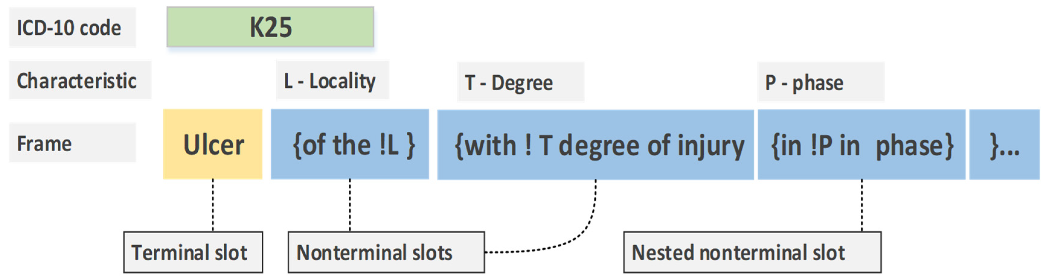
Figure 2.
UCSCD slot structure.
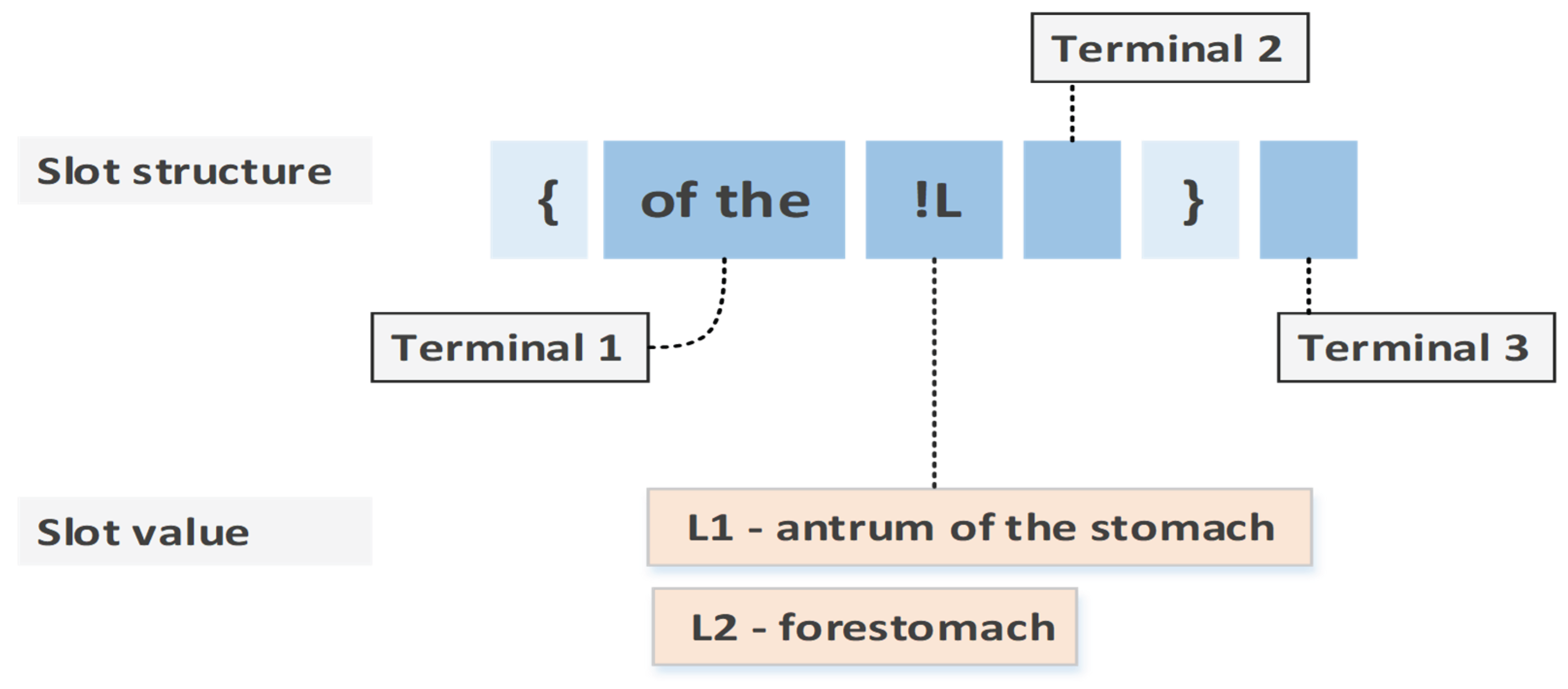

Table 1.
Assessment Scale for Cognitive Complexity of Test (tci).
| Score | Complexity Level | Description and Indicators |
| Cognitive Complexity of Test (tcj) | ||
| 1–2 | Baseline | Minimal Friction. Standard state verification with clearly defined inputs and outputs. No external environment setup is required. |
| 3–5 | Medium | Environmental Friction. Requires specific state preparation (e.g., legacy FoxPro tables, specific SQL dialects, data sets). Demands deep knowledge of legacy data structures [23]. |
| 6-8 | High | Testing complex object graphs or moderately nested structures, which requires partial reconstruction of system state to verify a single test case. |
| 9–10 | Extreme | Cognitive Saturation. Testing recursive structures or complex object graphs where a single test forces the verification of the entire hierarchy [22] . |
| Cognitive Complexity of Data Access (dcp) | ||
| 1–2 | Baseline | Standard Access. Direct mapping using modern ORM/ADO.NET providers. |
| 3–5 | Medium | Environmental Friction. Working with legacy SQL dialects (e.g., FoxPro-specific SQL) or flat tables without relational integrity [23]. |
| 6–8 | High | Data access through low-level file operations with predictable, documented behavior. |
| 9–10 | Extreme | Structural Entropy. Accessing data through low-level file manipulations, proprietary drivers with side effects. |
| Monitoring Complexity (mcj) | ||
| 1–2 | Baseline | High Observability. Integrated logging frameworks provide full stack traces. State can be inspected via standard debugger without side effects. |
| 3–5 | Medium | Limited Visibility. Requires manual insertion of logging entries to track data flow through legacy components. Debugging is hindered by proprietary drivers or asynchronous boundaries [24]. |
| 6–8 | High | Limited observability, requiring custom diagnostic tools outside standard tooling. |
| 9–10 | Extreme | Black Box. System state is opaque. Developer must write custom visualization tools or use high-density debug and logging points to verify complex side effects [24]. |
Source: compiled by the authors
Table 2.
Approximate Cognitive Load (CC).
| Score | Level | Description | Example (Migration Context) |
| 1 | Trivial | Direct pass-through of business rules. No change in data structure or logic flow. | Simple logic, trivial tasks. |
| 2–3 | Linear | Logic remains flat and predictable and can be mapped onto target platform with minimum efforts. | Validation of intermediate business rules. |
| 4–5 | Functional | Transition requires restructuring logic flow. Cannot be easily mapped from source platform onto target one. | Implementation of non-trivial algorithmic transformations. |
| 6–7 | Structural | Transition requires significant effort related to structural modifications (e.g. shift in data topology). | Implementing recursive mapping for ICD classes tree with up to 4 levels of nesting. |
| 8–9 | Complex | Original complex logic which requires significant effort to realize the task. Paradigm shift. | Working with hierarchical knowledge structures. |
| 10 | Extreme | Architectural Gravity: Unpredictable flow due to extreme complexity of task or legacy side effects. | We don't have such logic in the presented projects |
Source: compiled by the authors
Table 3.
Coupling factor scale (CF).
| Score | Level | Description | Example |
| 1-2 | Isolated | Method works with primitive types or local DTOs. No dependency on legacy state. | Math utility or internal string formatter. |
| 3-5 | Domain Bound | Dependent on modern domain entities but isolated from the legacy database. | ICD classification hierarchy management without direct SQL calls. |
| 6-8 | Environment Bound | Tight coupling with legacy database schemas. | Frame collection retrieval |
| 9-10 | Global State Bound | Dependency on side effects, shared legacy buffers, or non-deterministic external states. | We don't have such logic in the presented projects |
Source: compiled by the authors
Table 4.
Team unfamiliarity with the product (PIF, MIT, MIS).
| Score | Level | Description | Example |
| 1-2 | Native | Full support by modern frameworks. The team is acquainted with the technology. | Standard operations, known tasks. |
| 3-5 | Adapters, average complexity of domain | Requires wrappers or adapters. Synthetic solution. | FoxPro-specific SQL queries for .NET developers. |
| 6-8 | Complex domain or unknown technology | Requires deep understanding of the domain, source and target technological stacks. | Unknown OpenXML technology |
| 9-10 | Incompatible or unknown complex technologies applied to very high complexity tasks | Requires significant efforts to find a proper solution to the task. Always connected with research and experiments. | We don't have such tasks in presented projects. |
Source: compiled by the authors
Table 5.
The classification of the Print UCSCD steps by CAF levels.
| # | Use Case Step | Complexity Amplifier Factor |
| 1 | Input range (C11-C45) | Low: Involves routine string parsing and basic input query validation. |
| 2 | Translate to SQL | Low: Relies on Regular Expressions and standard string splitting algorithms to construct SQL queries. |
| 3-4 | Get Frames & Slots | Medium: Complicated by the need to map semi-structured frame-slot models and handle legacy Visual FoxPro-specific SQL dialect constraints. |
| 5 | Connect Slots to Frames | High: Effort diverges due to the overhead of building the aggregate object graph. Requires gathering and ordering relational slots based on unstructured textual frame descriptions. |
| 6 | Get ICD tree and attach Frames to Icd diagnoses | High: Transforming a flat relational table structure into a deeply hierarchical data structure using the Composite architectural design pattern. The mapping logic requires handling two interdependent recursions. |
| 7 | Translate to Word | Extreme: Requires mapping of the hierarchical ICD structure containing UCSCD clinical diagnosis frames into low-level OpenXML considering specifics of technology. |
Source: compiled by the authors
Table 6.
Results of the use case effort estimation using the baseline method µ(sk) and its modified version µ+(sk).
Table 6.
Results of the use case effort estimation using the baseline method µ(sk) and its modified version µ+(sk).
| Nested use case | μ | μ+ | Complexity amplifier factor | Approx. Effort (m-h) |
|||||
| 1-2 | 14 | 14 | 1.0 | - | - | - | 2 | 0.14 | 0.14 |
| 3-4 | 15 | 42 | 2.8 | 1 | - | 0.8 | 4 | 0.26 | 0.1 |
| 5 | 25 | 87.5 | 3.50 | 1 | 1.5 | - | 8 | 0.32 | 0.09 |
| 6 | 25 | 108.75 | 4.35 | 1.25 | 1.9 | 0.2 | 10 | 0.4 | 0.09 |
| 7 | 40 | 398 | 9.95 | 1.25 | 2.5 | 5.2 | 46 | 1 | 0.12 |
| Total | 119 | 650.25 | Avg(αM)=4.32 | 70 | 0.58 | 0.11 | |||
Source: compiled by the authors
Table 7.
The individual component values and the resulting aggregated CAF metrics for each step.
| Nested use case | Complexity amplification factor | |||||||||
| tc | dc | mc | cc | r | cr | pif | mit | mis | ||
| 1-2 | 1.0 | 1 | - | - | - | - | - | - | - | - |
| 3-4 | 2.8 | 1 | 3 | 1 | - | - | - | 2 | - | 4 |
| 5 | 3.50 | 1 | 3 | 1 | 5 | - | 5 | - | - | - |
| 6 | 4.35 | 2 | 3 | 1 | 5 | 2 | 2 | 3 | 0 | 1 |
| 7 | 9.95 | 2 | 3 | 1 | 6 | 1 | 6 | 7 | 8 | 3 |
Source: compiled by the authors
Table 8.
The prediction results for both methods (CAF-enhanced method and the standard one).
| Nested use case | | Predicted (=0.11) | Relative Error (MRE+) | using Гi | MRE+ | Predicted (=0.58) | Relative Error (MRE) | using Гi | MRE | |
| 1-2 | 2 | 14 | 1.5 | 0.25 | - | - | 8.12 | 3.06 | - | - |
| 3-4 | 4 | 42 | 4.5 | 0.12 | 6 | 0.5 | 8.7 | 1.18 | 2.14 | 0.46 |
| 5 | 8 | 87.5 | 9.4 | 0.18 | 9.38 | 0.17 | 14.5 | 0.81 | 5.17 | 0.35 |
| 6 | 10 | 108.75 | 11.7 | 0.17 | 10.61 | 0.06 | 14.5 | 0.45 | 6.48 | 0.35 |
| 7 | 46 | 398 | 42.7 | 0.07 | 37.87 | 0.18 | 23.2 | 0.5 | 12.15 | 0.74 |
| h = 69.8 = 0.158 |
= 0.227 | h = 69.02 MMRE = 1.199 |
MMRE = 0.476 | |||||||
Source: compiled by the authors
Table 9.
The main use cases of the UCSCD editor project.
| Use case | Abbreviation | xUUSP | Anomaly |
| GetIcdClassification | GIC | 115 | Middle |
| RegisterIcdClass | RIC | 42 | Middle |
| RegisterIcdDiagnosis | RID | 13 | Middle |
| ChangeIcdClassName | CICN | 15 | Low |
| ChangeIcdDiagnosisName | CIDN | 7 | Low |
| GetAxisCollection | GAC | 16 | Low |
| GetFrame | GF | 68 | High |
| SaveFrame | SF | 25 | High |
| RemoveFrame | RF | 5 | Low |
Source: compiled by the authors
Table 10.
The prediction results for the functions with CAF > 0.
| Steps Block | CAF | Appr. Effort (m-h) |
|||||||
| GIC | 115 | 184 | 1.6 | - | 0.6 | - | 8 | 0.07 | 0.044 |
| RIC | 42 | 212.1 | 5.05 | 1.25 | 1.2 | 1.6 | 8 | 0.19 | 0.038 |
| RID | 13 | 51.35 | 3.95 | 0.75 | 0.9 | 1.3 | 2 | 0.154 | 0.039 |
| GF | 68 | 255 | 3.75 | 1.25 | 1.5 | 0 | 12 | 0.176 | 0.047 |
| SF | 25 | 158.75 | 6.35 | 1.25 | 2.1 | 2.0 | 10 | 0.400 | 0.063 |
| Total | 263 | 861 | 40 | 0.198 | 0.046 | ||||
Source: compiled by the authors
Table 11.
Prediction accuracy for use cases (Table 10).
Table 11.
Prediction accuracy for use cases (Table 10).
| Nested use case | | (=0.046) | Relative Error (MRE+) | using Гi | MRE+ | (=0.2) | Relative Error (MRE) | using Гi | MRE |
| GIC | 8 | 8.5 | 0.063 | - | - | 23 | 1.88 | - | - |
| RIC | 8 | 9.8 | 0.225 | 9.22 | 0.15 | 8.4 | 0.05 | 2.92 | 0.64 |
| RID | 2 | 2.4 | 0.2 | 2.07 | 0.04 | 2.6 | 0.3 | 1.32 | 0.34 |
| GF | 12 | 11.7 | 0.025 | 10.26 | 0.15 | 13.6 | 0.13 | 7.2 | 0.4 |
| SF | 10 | 7.3 | 0.27 | 6.78 | 0.32 | 5 | 0.50 | 3.15 | 0.69 |
| h = 39.7 MRE = 0.157 (15.7%) |
MMRE+= 0.164 | h = 52.6 MRE = 0.572 |
MMRE = 0.514 | ||||||
Source: compiled by the authors
Disclaimer/Publisher’s Note: The statements, opinions and data contained in all publications are solely those of the individual author(s) and contributor(s) and not of MDPI and/or the editor(s). MDPI and/or the editor(s) disclaim responsibility for any injury to people or property resulting from any ideas, methods, instructions or products referred to in the content. |
© 2026 by the authors. Licensee MDPI, Basel, Switzerland. This article is an open access article distributed under the terms and conditions of the Creative Commons Attribution (CC BY) license.
Copyright: This open access article is published under a Creative Commons CC BY 4.0 license, which permit the free download, distribution, and reuse, provided that the author and preprint are cited in any reuse.