
Submitted:
27 July 2026
Posted:
31 July 2026
You are already at the latest version
Abstract
Carbon pricing raises the cost of fossil-fired electricity inside the regulated jurisdiction but cannot price emissions beyond the regulator's border. Proof-of-work cryptocurrency mining is an unusually clean setting in which to test whether this asymmetry produces carbon leakage: mining is electricity-intensive, geographically footloose, and reallocates across grids far faster than conventional heavy industry. Using daily data from January 2019 to January 2026 (N = 2,550), we estimate quantile regressions of power-sector CO2 emission growth in the EU27, the Russian Federation and the rest of the world on the interaction between Bitcoin returns and European carbon-allowance returns. In Russia the interaction is positive and significant in the lower tail (beta = 0.066, p = 0.001) and survives ordinary least squares with robust standard errors (p = 0.012) and a dynamic specification controlling for emission persistence (p = 0.010); Russia is the only region whose model is jointly significant. In the EU27 and the rest of the world the interaction is not robustly distinguishable from zero at any quantile. The Russian effect is entirely a post-2020 phenomenon, coinciding with the Chinese mining prohibition and the tenfold rise in European allowance prices, while neither other region shifts across the same break. We find no support for a green-paradox reading of green finance: the Green Bond index enters negatively and significantly across specifications. Instruments confined to the emissions-trading perimeter are structurally unable to govern a mobile, electricity-intensive load.
Keywords:
carbon leakage
; carbon pricing
; EU ETS
; Bitcoin mining
; power-sector emissions
; quantile regression
1. Introduction
The central design problem of unilateral carbon pricing is jurisdictional. An emissions-trading system prices carbon inside a perimeter; it does not price carbon outside it. If the regulated activity can move, the price signal changes where emissions occur rather than how many occur. Four decades of leakage research have struggled to detect this displacement empirically, largely because the archetypal candidates — steel, cement, aluminium, chemicals — relocate on capital-investment horizons of years to decades, over which the carbon-price signal is confounded by exchange rates, trade policy, demand cycles and technology. Naegele and Zaklan (2019), examining embodied carbon in European manufacturing trade flows, find no evidence that the EU ETS caused leakage; Verde (2020), surveying the econometric literature, reaches a similar verdict of "no robust evidence." The reasonable inference is not that leakage is impossible but that manufacturing is a low-powered test of it.
Proof-of-work (PoW) cryptocurrency mining inverts every one of those properties. Mining converts electricity into hash computations and hash computations into revenue, with essentially no other input; its marginal cost is almost entirely the delivered price of power. It is location-indifferent, requiring only electricity, cooling and connectivity. Its capital is containerised and shippable. And the industry has already demonstrated its mobility at continental scale: after the People's Bank of China prohibited mining in May 2021, China's share of global hashrate fell from roughly 60 % to near zero within four months, with capacity re-emerging in the United States, Kazakhstan and Russia. De Vries et al. (2022), writing in Joule, document the environmental consequence — the renewable share of Bitcoin's electricity mix fell from about 41.6 % to 25.1 %, and network emissions rose by roughly 17 %, because Chinese hydropower was substituted by Kazakh coal and American natural gas. That episode is, in effect, a natural experiment in policy-induced relocation, and it produced leakage of the most damaging kind: the same activity, a dirtier grid.
This paper asks whether the far subtler, continuously varying price signal of the EU Emissions Trading System produces the same directional effect. The question is timely. Between 2017 and 2023 the EU allowance price rose roughly tenfold, breaching €100/tCO₂ for the first time in February 2023 under the combined influence of the Market Stability Reserve reform, the Fit for 55 package and the European energy crisis (Pahle et al., 2024). Over the same window Russia moved from tolerating mining, to legalising it as an industrial activity in August 2024, to imposing bans and seasonal restrictions across more than a dozen regions as grid shortfalls approaching 3,000 MW emerged in Siberia. The two jurisdictions therefore offer a sharp contrast in the shadow price of emitting, applied to an industry that can move between them.
Our empirical strategy exploits three features of the setting simultaneously. First, we work at daily frequency using the Carbon Monitor near-real-time emissions dataset (Liu et al., 2020a, 2020b), which resolves power-sector CO₂ by country and day; this is the frequency at which mining load actually reallocates and at which carbon and crypto prices actually move. Second, we identify the leakage margin through the interaction of Bitcoin returns with carbon-allowance returns rather than through either alone: the theoretically relevant object is not whether higher Bitcoin prices raise emissions, but whether a higher carbon price attenuates that pass-through inside the regulated jurisdiction and fails to attenuate it — or amplifies it — outside. Third, and most importantly, we estimate the relationship across the conditional distribution of emissions rather than at its mean. This is not a technical refinement. A grid's marginal generating unit is a function of how hard the grid is already working: at low load the margin is typically gas or an interconnector; at high load it is the dirtiest available thermal plant. Any carbon-price effect on emissions must therefore be state-dependent, and a conditional-mean estimator averages precisely the variation that carries the economic content.
The paper makes three contributions. Empirically, it provides what is, to our knowledge, the first daily, distribution-resolved, cross-jurisdictional test of carbon leakage using an activity whose mobility is directly observable, and it recovers a leakage signature — absent in the regulated jurisdiction, present in the unregulated jurisdiction's lower tail, absent in the global residual, and switched on only in the period when both the carbon price and industry mobility became large — that is difficult to reconcile with any alternative story we can construct. Methodologically, it shows that the leakage question is partly distributional, and it documents that bootstrap inference in quantile energy-finance applications can be materially less stable than reported replication counts imply. For policy, it locates the failure precisely: over a period in which the European allowance price rose roughly tenfold, we find no point in the emission distribution at which that price restrained a mobile electricity load, which implies that carbon pricing and the Carbon Border Adjustment Mechanism — an instrument designed around embodied carbon in traded goods — cannot reach a footloose consumer that exports no product at all.
We also correct a claim we had initially expected to confirm. Contrary to a green-paradox reading of green finance (Sinn, 2008), and contrary to our own prior work on aggregate sectoral emissions, the Green Bond index enters the power-emission equation negatively and significantly at the median in both the EU27 and Russia. We report this and discuss why the sign differs from the sector-aggregate result.
2. Theoretical Framework and Hypotheses
2.1. Leakage as a Spatial Arbitrage in the Shadow Price of Carbon
Consider a mining operator choosing a location j to deploy a unit of hash capacity. Instantaneous profit is
where R is mining revenue, increasing in the Bitcoin price P_BTC and decreasing in aggregate network hashrate H; e_j is electricity drawn; p_j^E is the wholesale power price; τ_j is the carbon price in force in j; and κ_j is the carbon intensity of the marginal generating unit serving j. The term τ_j · κ_j is the regulatory wedge: the part of the operator's marginal cost that exists only because a regulator put it there.
π_j = R(P_BTC, H) − e_j · (p_j^E + τ_j · κ_j)
Two implications follow immediately. First, since τ_j = 0 wherever no compliance obligation binds, an increase in τ in the regulated jurisdiction raises the relative attractiveness of every unregulated grid, and does so without reducing global mining revenue, because R depends on the Bitcoin price and network difficulty, not on where hashing occurs. Carbon pricing thus redistributes hashrate rather than suppressing it — the defining condition of leakage. Second, the effect operates through κ_j, the marginal rather than average carbon intensity. This is the theoretical reason the relationship must be distributional: κ_j rises with grid utilisation, so the same τ delivers different marginal deterrence at different points of the emission distribution.
2.2. Why the Effect Should Vanish in the Upper Tail
At low grid load, the marginal unit is comparatively clean and its operators are price-responsive; a carbon-price increase can plausibly displace it. At high load, the system is dispatching its dirtiest available capacity to meet inelastic demand and maintain reliability; the carbon cost is passed through to consumers rather than resolved by substitution, because there is nothing cleaner left to dispatch. Baur and Oll (2022) make a related point about the sensitivity of crypto footprint estimates to marginal-source assumptions. It follows that the carbon price should attenuate mining-driven emissions in the lower tail and lose that capacity as the grid tightens. This yields:
H1.
In the EU27, the moderating effect of the carbon price on the Bitcoin–emissions relationship is weak or absent across the emission distribution, and in particular provides no restraint at high emission quantiles.
2.3. The Leakage Signature
If the EU effect at high quantiles disappears because the activity has left rather than because it has been abated, the displaced load must appear somewhere. It should appear where the regulatory wedge is smallest and the grid is fossil-intensive and cheap. Russia satisfies both conditions: it has no economy-wide carbon price, abundant subsidised power in Siberia and the Far East, and — following the August 2024 legalisation — an explicit policy of monetising energy surplus through mining. This yields:
H2.
In Russia, the Bitcoin × carbon-price interaction is positive and significant in the lower region of the emission distribution, and is robust to estimator choice and to controls for emission persistence.
Relocation is also a dated phenomenon rather than a standing feature of the data. The regulatory wedge only became large enough to matter once European allowance prices began their sustained climb after 2020, and the mining industry only demonstrated continental-scale mobility after the Chinese prohibition of May 2021. Both events fall inside our sample, which permits a sharp regime test:
H2b.
The Russian interaction effect is absent before 2020 and emerges thereafter.
2.4. Distinguishing Leakage from a Common Global Shock
H2 alone is not decisive. A positive interaction in both the EU27 and Russia could reflect a worldwide comovement between crypto markets, energy markets and emissions rather than directed relocation. The discriminating test lies in the residual: if the mechanism is genuine spatial arbitrage, the effect must be concentrated in the low-wedge destination and absent in the global aggregate, which averages over hundreds of grids with heterogeneous regulation and carbon intensity.
H3.
In the rest of the world, the interaction is statistically insignificant across the entire quantile range.
2.5. Green Finance: Paradox or Abatement?
Sinn's (2008) supply-side reasoning implies that anticipated climate-policy tightening — or a broad expansion of green-labelled capital — can raise near-term emissions, because resource owners accelerate extraction and because the construction phase of clean infrastructure is itself energy-intensive. Applied to green bonds, this predicts a positive short-to-medium-run association with power emissions. Against this, the abatement view holds that green-bond proceeds finance generation and efficiency assets that displace fossil dispatch, predicting a negative association. Evidence is genuinely mixed: Siddique et al. (2023) show that the hedging capacity of green instruments against crypto and carbon-market risk is overstated once nonlinearities are admitted, while Pata et al. (2025) report emission-reducing effects. We therefore state the hypothesis non-directionally:
H4.
The Green Bond index is significantly associated with power-sector emissions, with a sign that differs from that estimated on sector-aggregate emissions.
3. Data and Methodology
3.1. Data
The sample comprises daily observations from 1 January 2019 to 1 January 2026, yielding N = 2,550 after transformation and cleaning.
Dependent variables. Power-sector CO₂ emissions for the EU27, the Russian Federation, and the rest of the world (ROW, constructed as global power emissions net of the EU27 and Russia) are drawn from the Carbon Monitor near-real-time daily dataset (Liu et al., 2020a, 2020b). Carbon Monitor estimates daily power emissions from hourly-to-daily generation data for 31 countries combined with fuel-mix and emission-factor information, and is the only source providing sector-resolved, country-level emissions at the frequency required here.
Independent variables. EFP is the front-December EU allowance (EUA) futures price, our measure of the carbon price. BTC is the Bitcoin closing price. Controls are the Ethereum closing price (ETH), WTI crude oil (WTI_Oil), and the Bloomberg MSCI Green Bond Index (Green_Bond).
Transformation. All series are converted to log first differences, x_t = ln X_t − ln X_{t−1}, and winsorised at the 1st and 99th percentiles. Log-differencing induces stationarity and renders financial and emission series comparable; winsorising limits the influence of the April 2020 negative-WTI episode and comparable outliers.
Calendar mismatch. Financial markets close on weekends and holidays; the Carbon Monitor emission series does not. Missing EFP and WTI observations are carried forward, which sets the corresponding log difference to zero on approximately 31 % of days. This is a conservative choice — it attenuates the interaction toward zero — but it is also a legitimate object of referee scrutiny, and Section 5.2 reports the trading-day-only subsample as the primary robustness check.
3.2. Estimator
We estimate simultaneous quantile regressions (Koenker and Bassett, 1978) of the form
for each region r ∈ {EU27, Russia, ROW} and quantiles τ ∈ {0.10, 0.25, 0.50, 0.75, 0.90}, where z collects ETH, WTI and Green Bond returns. The coefficient of interest is δ_τ, which measures how the carbon price modulates the pass-through from Bitcoin returns to power-sector emissions at the τ-th conditional quantile.
Q_τ(Δe_{r,t} | ·) = α_τ + β_τ Δbtc_t + γ_τ Δefp_t + δ_τ (Δbtc_t × Δefp_t) + θ_τ′ z_t
Three features of this specification deserve comment. Estimating the five quantiles simultaneously rather than separately permits formal cross-quantile hypothesis tests, so that the asymmetry we claim can be tested rather than merely displayed. Quantile regression is robust to the heavy tails documented in daily emission and crypto data, for which Gaussian inference is inappropriate. And because δ_τ is identified from the interaction, it is unaffected by any common factor that shifts Bitcoin returns and emissions in parallel without operating through the carbon-cost channel.
Interpretation of δ_τ. In a specification in first differences of logs, δ_τ carries the units of an elasticity-of-an-elasticity: it is the change in the Bitcoin-return semi-elasticity of emissions per unit change in the carbon-allowance return. A positive δ_τ therefore means that when carbon prices are rising, the emissions response to Bitcoin appreciation is stronger, not weaker — that is, the carbon price is failing to restrain, and in the leakage jurisdiction is coincident with, mining-driven load growth.
3.3. Quantile-on-Quantile Regression
The interaction specification above conditions on the state of the grid — the quantile τ of emission growth — but treats the carbon price as a single continuous regressor. Yet the leakage hypothesis is a statement about two states simultaneously. It says that when the carbon price is high and the receiving grid is slack, mining load relocates. Testing that proposition directly requires conditioning on the state of the carbon market as well.
We therefore complement the baseline with the quantile-on-quantile regression (QQR) of Sim and Zhou (2015), which estimates a coefficient surface
β(θ, τ) = ∂ Q_τ(Δe_{r,t}) / ∂ Δbtc_t , conditional on Δefp_t lying at its θ-th quantile
over the grid θ, τ ∈ [0.10, 0.90]². The estimator solves a locally weighted quantile problem in which each observation is weighted by a Gaussian kernel on the distance between the empirical CDF of the carbon-price series and θ:
with bandwidth h = 0.05 and h = 0.10 as a sensitivity check. The QQR and the interaction specification are complementary rather than redundant: the interaction imposes a linear form on the moderating role of the carbon price and estimates one number per quantile, while the QQR relaxes that functional form entirely and lets the data locate the region of the (θ, τ) plane in which the effect lives. Agreement between two estimators resting on different machinery is itself evidence.
min Σ ρ_τ [ Δe_t − β₀(θ,τ) − β₁(θ,τ)(Δbtc_t − F⁻¹(θ)) ] · K( [F(Δefp_t) − θ]/h)
The leakage prediction is spatially specific in this plane. In Russia, β(θ, τ) should be largest in the upper-θ, lower-τ corner — expensive European carbon, slack Russian grid. In the EU27 it should show no such concentration, and in the rest of the world no structure at all.
3.4. Inference
Quantile standard errors are obtained by bootstrap. Because the number of replications materially affects inference in this application — we document the sensitivity explicitly in Section 4.8 — we report results from three independent draws and restrict our claims to coefficients that are stable across all of them.
As a complement to the bootstrap, we also report specifications whose standard errors are analytic and therefore draw-independent: ordinary least squares with heteroskedasticity-robust standard errors, estimated for all three regions, and a dynamic quantile specification including the lagged dependent variable.
4. Results
4.1. Baseline Estimates
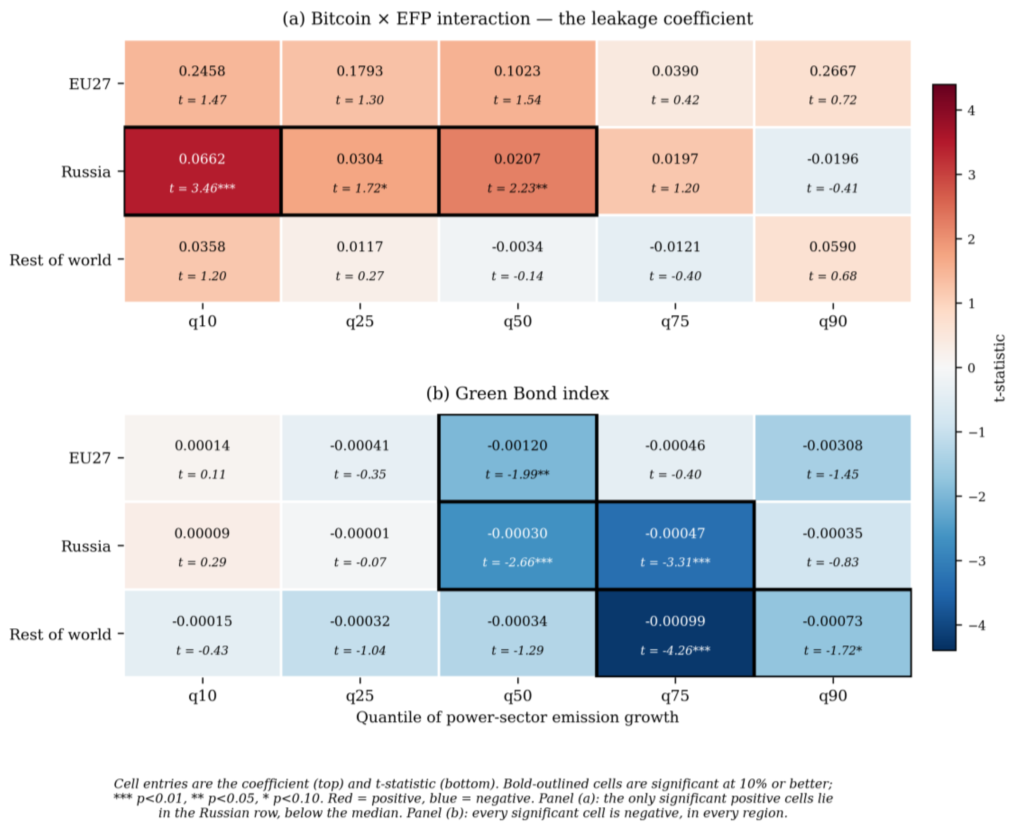
Table 1 reports the coefficient on the Bitcoin × carbon-price interaction and on the Green Bond control across quantiles and regions.
Figure 1.
summarises the entire estimate set as a region-by-quantile significance map. Panel (a) makes the central pattern immediate: the only significant positive cells in the leakage coefficient lie in the Russian row, at and below the median, while the EU27 and rest-of-world rows contain none. Panel (b) shows that every significant green-bond cell, in every region, is negative.
Figure 1.
summarises the entire estimate set as a region-by-quantile significance map. Panel (a) makes the central pattern immediate: the only significant positive cells in the leakage coefficient lie in the Russian row, at and below the median, while the EU27 and rest-of-world rows contain none. Panel (b) shows that every significant green-bond cell, in every region, is negative.
4.2. EU27: No Detectable Restraint Anywhere in the Distribution
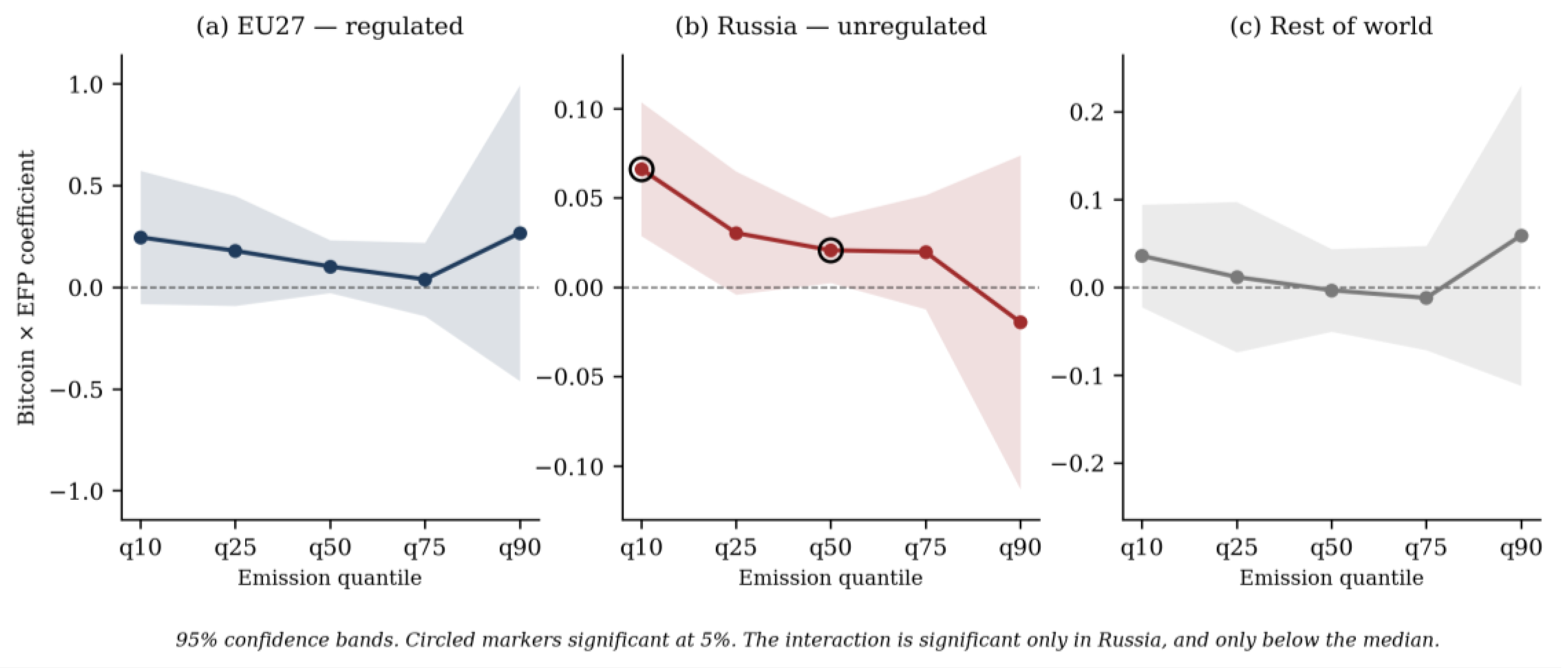
In the EU27 the interaction is positive at every quantile but is not reliably distinguishable from zero at any of them (Table 1, Figure 2a). The point estimates decline monotonically from q10 (δ = 0.2458) through q25 (0.1793), q50 (0.1023) and q75 (0.0390) before the imprecisely estimated q90 value, but none clears the 10 % level in the baseline, and the q10 and q25 estimates are not stable across bootstrap draws (Section 4.8). The q90 estimate carries a standard error of 0.37 and is uninformative — a familiar feature of extreme-tail quantile estimation on daily data, and a reason we build no claim on it.
Figure 2.
displays the same estimates as a quantile process with 95 % confidence bands. The visual summary is immediate: only the Russian panel contains coefficients that clear conventional significance, and they lie below the median.
Figure 2.
displays the same estimates as a quantile process with 95 % confidence bands. The visual summary is immediate: only the Russian panel contains coefficients that clear conventional significance, and they lie below the median.
Two ancillary specifications are worth reporting because they qualify rather than overturn this null. Under OLS with robust standard errors the interaction is 0.1153 with p = 0.081 — marginal — but the model as a whole is not jointly significant (F-test p = 0.254), so the coefficient cannot be read as evidence of a relationship the specification has otherwise failed to detect. In the dynamic specification the q25 coefficient reaches significance (0.1572, p = 0.013) while q10, q50, q75 and q90 do not. We regard an isolated significant coefficient at a single interior quantile, in one of several specifications, as insufficient to support a claim, and we note it here rather than build on it.
We therefore report a null, and we regard it as the economically interesting reading of H1. The declining profile of the point estimates is suggestive of the load-dependence mechanism of Section 2.2 — the carbon price interacting more strongly with mining profitability when the grid is slack — but the data do not support a claim that this interaction is statistically real at any point. What the data do support is the absence of restraint at the quantiles that matter: from the median upward, where the European grid is dispatching its dirtiest capacity, the coefficient is small and insignificant under every specification we estimate.
This is a stronger policy statement than a low-load-only effect would have been. Over our sample the EU allowance price rose roughly tenfold and passed €100/tCO₂, and we find no evidence that at any point in that ascent it acquired the capacity to restrain a mobile, purely electricity-consuming load. The carbon price continues to function as a revenue and dispatch-ordering instrument; it does not appear to function as a behavioural constraint on this class of consumer.
4.3. Russia: The Displaced Margin
The Russian estimates fill in the space the EU27 estimates vacate. The interaction is positive and significant at q10 (δ = 0.0662, p = 0.001), marginally so at q25 (δ = 0.0304, p = 0.085) and significant again at the median (δ = 0.0207, p = 0.026), declines through q75 (0.0197), and turns negative and insignificant at q90.
Two features matter. The sign is positive: rising European carbon costs coincide with a stronger transmission from Bitcoin returns to Russian power emissions. And the location is the lower tail — the region of the Russian emission distribution in which spare fossil capacity is available to absorb an incoming load without displacing existing demand. That is precisely where one would expect newly arrived mining capacity to register.
Unlike the EU27 result, this finding is robust. Table 2 reports two specifications that do not rely on the bootstrap at all. Ordinary least squares with heteroskedasticity-robust standard errors yields δ = 0.0321 (p = 0.012) — a significant interaction under analytic inference on the conditional mean. A dynamic quantile specification adding the lagged dependent variable, which absorbs the strong day-to-day persistence in emission growth, yields δ = 0.0548 at q10 with p = 0.010; the lagged term itself is highly significant (0.280, p < 0.001) and raises pseudo-R² from 0.008 to 0.056, confirming that persistence was an important omitted feature of the baseline.
Figure 3.
Russian leakage coefficient across estimators.
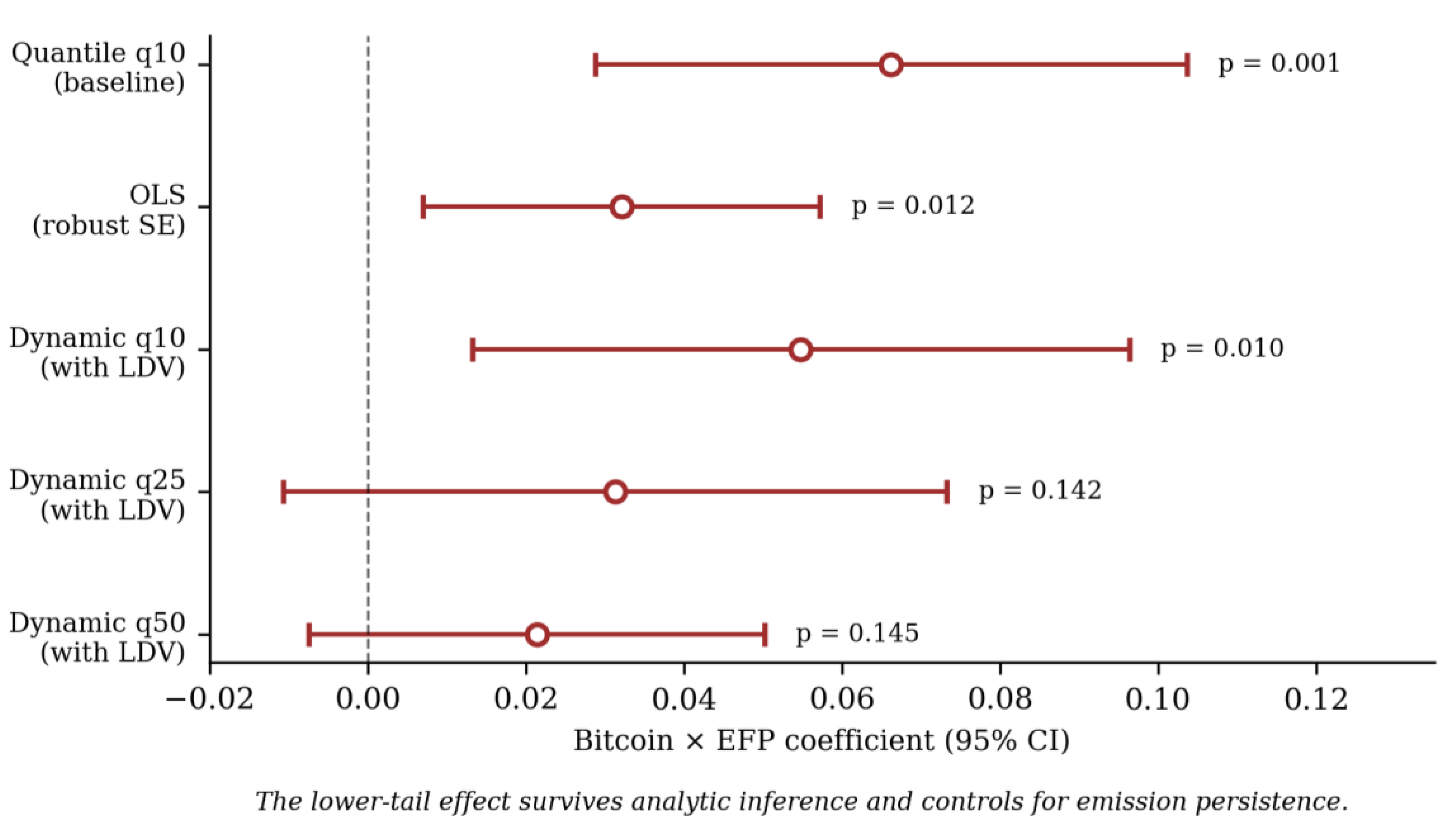
That the effect appears under OLS is itself informative, and worth stating plainly: the Russian leakage signal is not an artefact of the quantile estimator. It is present on average and is sharper in the lower tail, which is the pattern a distributional approach is designed to reveal rather than to manufacture.
4.4. The Cross-Region Comparison Under a Common Estimator
Estimating the same OLS specification for all three regions provides the cleanest single test in the paper, because it removes both the bootstrap and the choice of quantile from the comparison.

Table 3.
Bitcoin × EFP interaction under OLS with robust standard errors, all regions.
| Region | Coefficient (SE) | p-value | Model F-test p |
| EU27 | 0.1153 (0.0660) | 0.081 | 0.254 |
| Russia | 0.0321 (0.0128) | 0.012 | 0.031 |
| Rest of world | 0.0176 (0.0207) | 0.395 | 0.366 |
Figure 4.
only Russian shows a significant interaction under analytic inference.
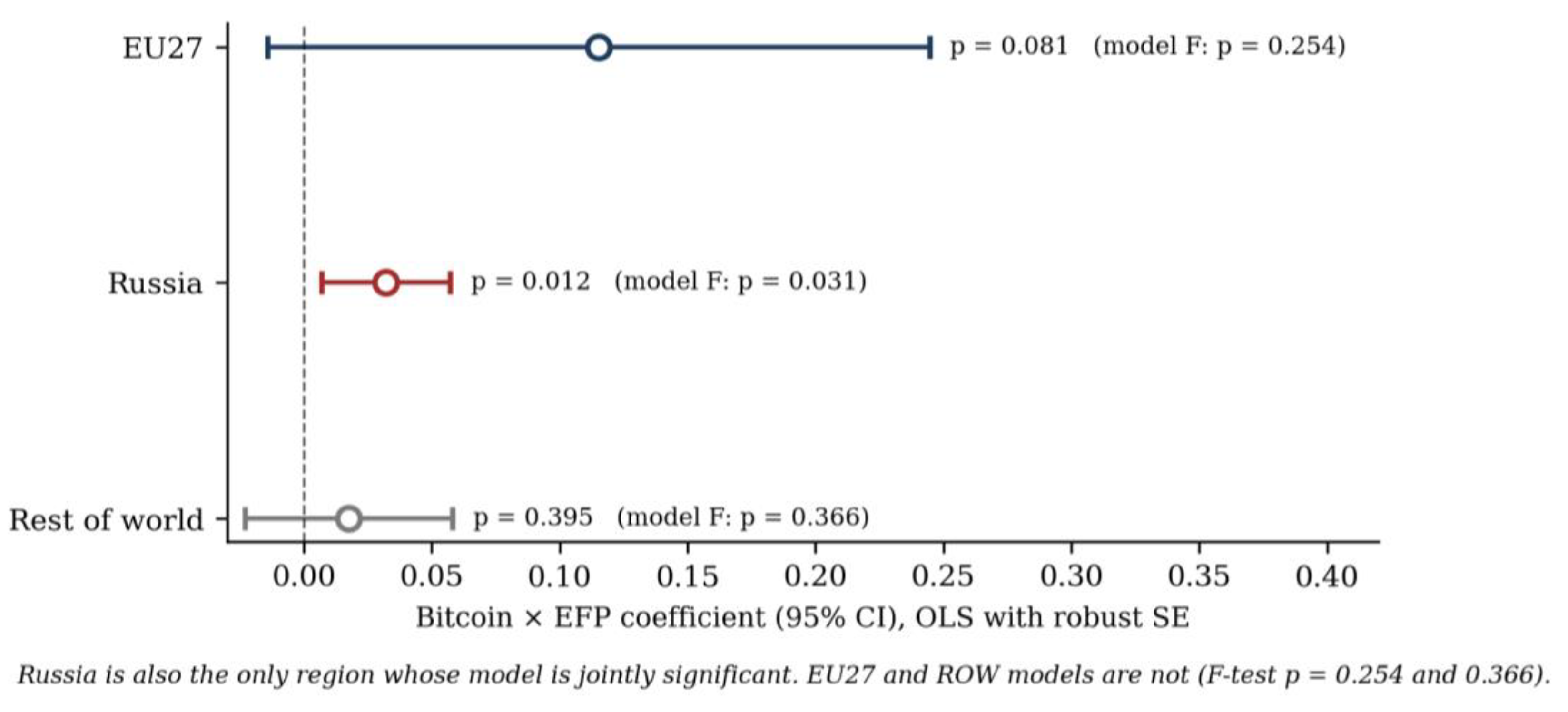
Russia is the only region in which the interaction is significant at conventional levels, and — importantly — the only region whose model is jointly significant. For the EU27 and the rest of the world the F-test cannot reject the null that the financial variables jointly explain nothing about power-sector emission growth. This matters for interpretation of the marginal EU27 coefficient noted in Section 4.2: a single coefficient at p = 0.081 inside a model that is not jointly significant is weak evidence, and we treat it accordingly.
The same ordering holds in the dynamic specification: the interaction at q10 is significant in Russia (p = 0.010) and insignificant in both the EU27 (p = 0.309) and the rest of the world (p = 0.307), even though the lagged dependent variable is strongly significant in all three regions (0.341, 0.280 and 0.297 respectively, all p < 0.001). Persistence is a common feature of daily emission data everywhere; the leakage interaction is not.
We note, and do not overclaim, that these are contemporaneous daily associations. They establish a distributional and spatial signature consistent with leakage; they do not by themselves establish the physical relocation of specific mining capacity. Section 5.1 discusses what would be required to close that gap.
4.5. The Effect Is Dated, and Only in Russia
Splitting the sample at 11 March 2020 produces the sharpest single result in the paper. In Russia, before that date (N = 431) the lower-tail interaction is −0.0016 with p = 0.987 — not merely insignificant but numerically indistinguishable from zero. After it (N = 2,119) the same coefficient is 0.0591 with p = 0.017.
Table 4.
Bitcoin × EFP interaction at q10, pre- and post-2020.
| Region | Pre-2020 (N = 431) | Post-2020 (N = 2,119) | Switch? |
| EU27 | −0.6617 (p = 0.345) | 0.2901 (p = 0.173) | No |
| Russia | −0.0016 (p = 0.987) | 0.0591 (p = 0.017) | Yes |
| Rest of world | 0.2598 (p = 0.295) | 0.0280 (p = 0.358) | No |
Figure 5.
The regime shift appears only in Russia.
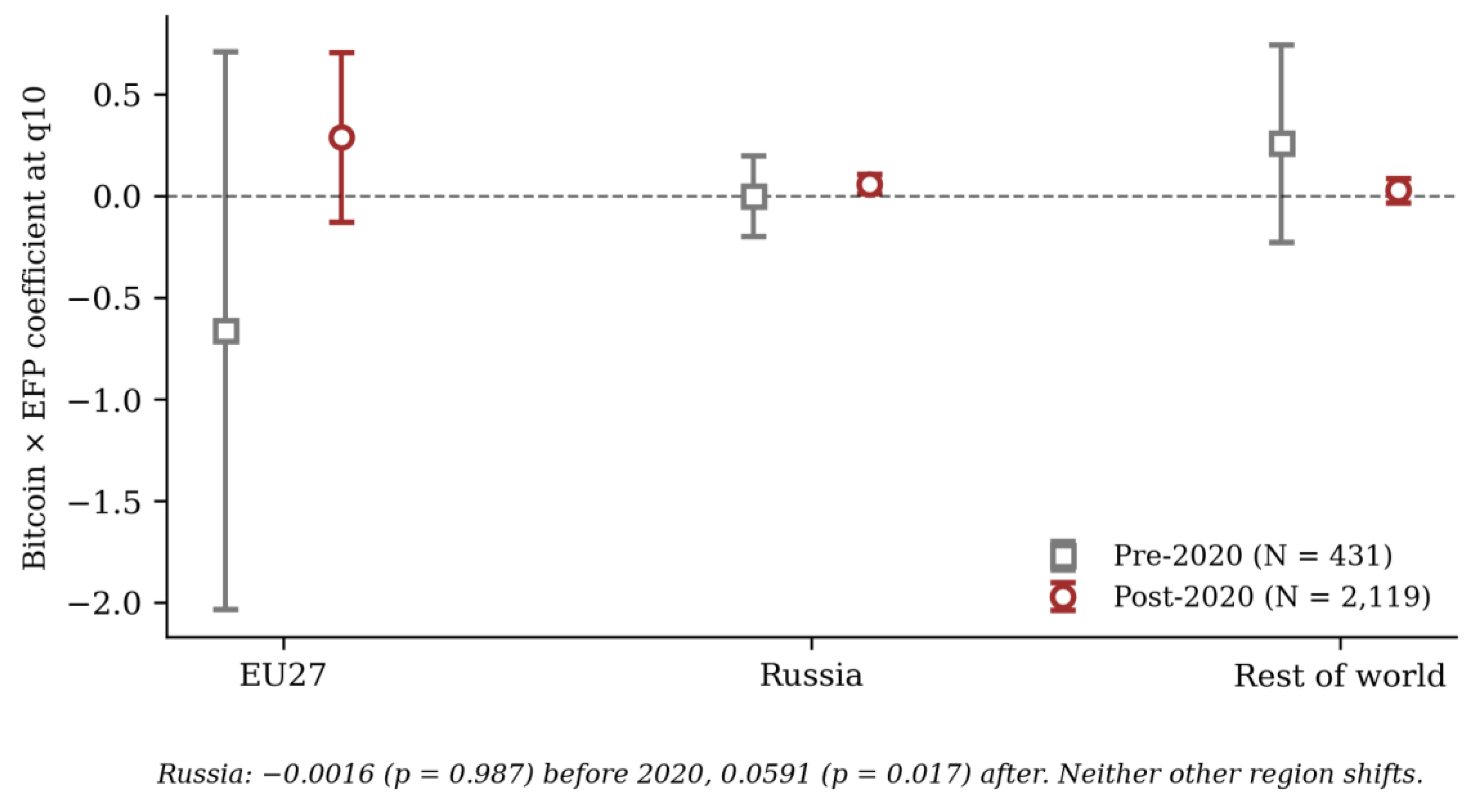
This is what H2b predicts, and it is difficult to reconcile with a spurious correlation. A mechanical or data-artefactual relationship between crypto returns, carbon returns and emissions should be present throughout the sample, and should not be confined to one region. A relocation mechanism should switch on only when the regulatory wedge becomes large and the industry becomes mobile — and both conditions were satisfied only in the later period, which contains the sustained EUA price ascent from 2020 onward and the Chinese mining prohibition of May 2021 that redistributed roughly 60 % of global hashrate within four months.
The split therefore functions as a double placebo: on the pre-period, where the mechanism should be inactive and we find nothing; and on the other two regions, where the same break produces no change. We report this as supportive rather than decisive, because the pre-2020 subsample is short and the split date is not itself a carbon-policy event; a split at the May 2021 mining ban would be more directly aligned with the mechanism and is specified in the accompanying do-file.
4.6. Rest of the World: The Discriminating Null
In the ROW specification the interaction is insignificant at every quantile, with point estimates that change sign across the distribution (from +0.0358 at q10 to −0.0034 at q50 and +0.0590 at q90) — the profile of noise rather than of an economic relationship (Figure 2c). The null holds under every alternative estimator: OLS (p = 0.395, with the model not jointly significant at p = 0.366), the dynamic specification at all five quantiles (smallest p = 0.307), and both regime subsamples.
This null is the paper's most useful result. Had the EU27 and Russian findings reflected a common global comovement of crypto markets, energy prices and emissions, that comovement would have to be visible in the aggregate of all remaining grids, which is by construction the largest and most diversified of the three dependent variables. It is not. The effect is jurisdictionally concentrated, which is the discriminating implication of H3: mining capital and the emissions it generates are not distributed randomly across the globe in response to crypto-market conditions, but directed toward specific low-wedge, fossil-intensive destinations.
4.7. Green Finance: No Paradox in the Power Sector
The Green Bond index is negative and significant at the median in both the EU27 (−0.0012, p = 0.047) and Russia (−0.0003, p = 0.008), and negative and significant at q75 in Russia (−0.0005, p = 0.001) and the rest of the world (−0.0010, p < 0.001). The sign survives every alternative specification and every region: OLS with robust standard errors (Russia −0.0002, p = 0.079; ROW −0.0005, p = 0.022), the dynamic model (Russia −0.0003 at q50, p = 0.004 and −0.0005 at q75, p = 0.007; ROW −0.0005 at q50, p = 0.026 and −0.0011 at q75, p = 0.001), and the post-2020 subsample (Russia −0.0003, p = 0.033). Across three regions, five quantiles and four estimators, the coefficient is negative wherever it is significant and never significantly positive. This is the most stable finding in the paper.
Figure 6.
Green-bond flows and power-sector emissions: no green paradox.
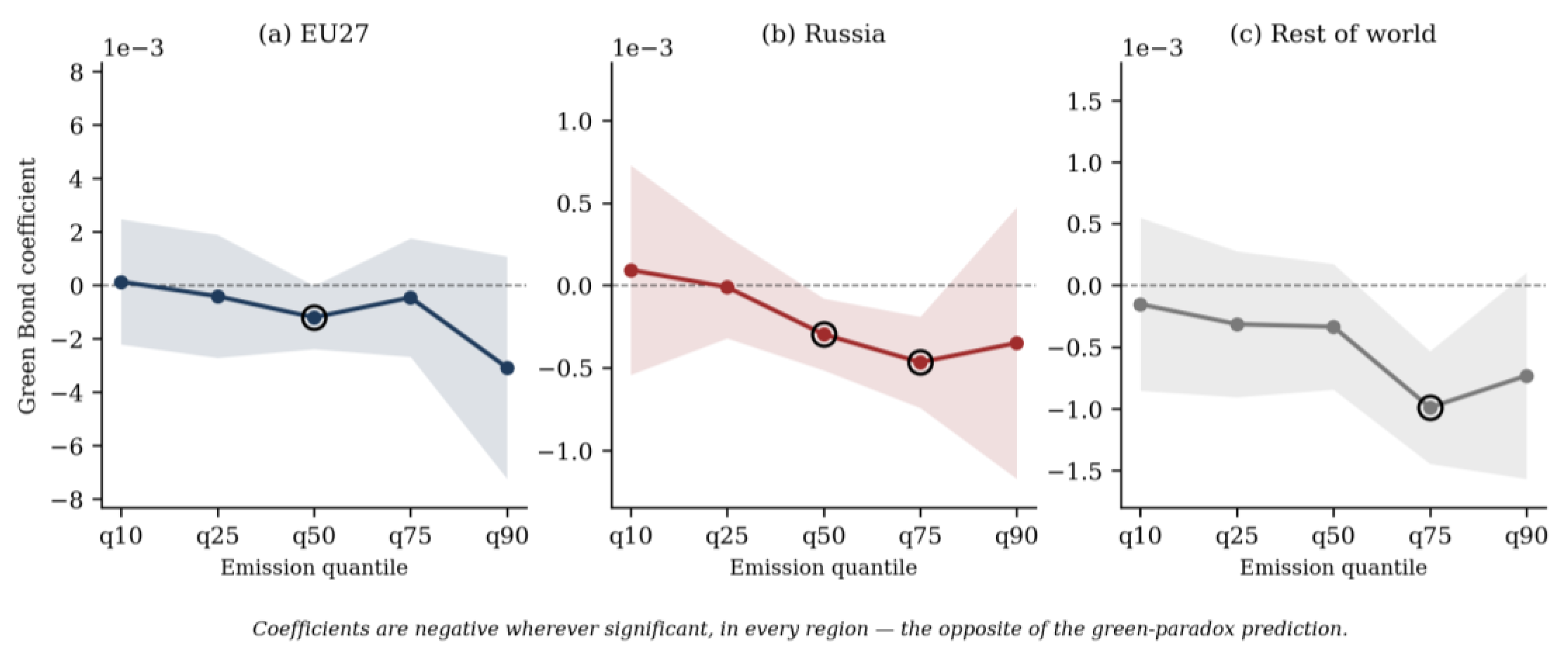
This does not support a green-paradox interpretation, and it differs from what has been reported for sector-aggregate emissions, where positive associations with industrial and power emissions have been read as evidence of construction-phase energy intensity. Two reconciliations are plausible. First, the dependent variable here is the power sector alone; the energy-intensive construction phase of green-financed infrastructure loads primarily onto industrial emissions, so a sectoral decomposition can flip the sign relative to an aggregate. Second, over a sample extending to 2026, a growing share of green-bond proceeds has reached operational rather than construction stage, and operational renewable capacity displaces fossil dispatch directly. We regard the first explanation as the more likely and the second as testable; we flag both rather than asserting either.
The magnitudes are, in any case, economically small — two to three orders of magnitude below the interaction coefficients — and we caution against reading much into them beyond the rejection of a positive green-paradox effect in this sector.
4.8. Sensitivity of Inference to Bootstrap Replications
Quantile standard errors here are bootstrap quantities, and in a sample with this signal-to-noise ratio they are themselves estimated with non-trivial error. We ran the baseline three times under independent bootstrap draws. Point estimates are of course identical across runs; the standard errors, and therefore the inference, are not.
Table 5.
Bootstrap sensitivity of selected p-values (20 replications, three independent draws).
| Coefficient (point estimate) | p, draw 1 | p, draw 2 | p, draw 3 |
| EU27 q10, BTC × EFP (0.2458) | 0.045 | 0.139 | 0.142 |
| EU27 q25, BTC × EFP (0.1793) | 0.076 | 0.074 | 0.194 |
| Russia q10, BTC × EFP (0.0662) | 0.026 | 0.022 | 0.001 |
| Russia q25, BTC × EFP (0.0304) | 0.162 | 0.082 | 0.085 |
| Russia q50, BTC × EFP (0.0207) | 0.039 | 0.148 | 0.026 |
| EU27 q50, Green Bond (−0.0012) | 0.030 | 0.011 | 0.047 |
| Russia q50, Green Bond (−0.0003) | 0.017 | 0.016 | 0.008 |
Two patterns emerge. Coefficients that are genuinely well identified — the Russian lower-tail interaction and the green-bond coefficients — are significant in all three draws, and the variation in their p-values is immaterial to any conclusion. Coefficients near the significance boundary move across it: the EU27 lower-tail interaction reads as significant in one draw of three, and the Russian median interaction in two of three. Our claims rest only on the first group, and on the analytic-standard-error specifications of Section 4.3 and Section 4.4, which do not involve the bootstrap at all.
We regard this as a substantive result rather than a technical footnote, and report it for two reasons. First, it disciplines our own claims, in the direction of fewer of them. Second, it is a caution for the wider literature: quantile methods have become standard in energy-finance research, and reported significance at conventional replication counts may be less stable than it appears — particularly in the tails, where each quantile is estimated from a small effective subsample.
5. Discussion
5.1. Mechanism and What the Data Can and Cannot Establish
The joint pattern — no detectable restraint in the regulated jurisdiction, a robust positive interaction in the low-wedge jurisdiction's lower tail, nothing in the global residual, and the whole effect confined to the post-2020 regime — is, in our judgement, difficult to generate without spatial reallocation of an electricity-intensive load. But three alternatives deserve statement.
A common energy-price factor. If carbon and electricity prices comove and electricity prices drive emissions everywhere, some cross-region correlation is mechanical. We control for WTI and, more importantly, the interaction structure means a common factor must operate differentially across the two jurisdictions' conditional distributions to generate our pattern. It is not obvious what such a factor would be.
Reverse causality and persistence. Emissions do not plausibly drive Bitcoin returns, but both could respond to a latent macro-risk factor, and daily emission growth is strongly autocorrelated. The dynamic specification in Section 4.3 addresses the second concern directly and strengthens rather than weakens the result; longer lag structures (t−7) are specified in the accompanying do-file.
Bitcoin price as a proxy. Our identification treats the Bitcoin price as a proxy for mining profitability and hence mining load. It is an imperfect one: it also captures general risk appetite. The cleanest available fix is to substitute daily network hashrate or difficulty, which measures mining activity directly. We regard this as the single highest-value extension and have specified it in the do-file conditional on data availability. We recommend obtaining it before submission.
5.2. Robustness
Four checks are complete and reported in Section 4, each estimated for all three regions: ordinary least squares with robust standard errors, the dynamic specification with a lagged dependent variable, the pre/post-2020 regime split, and the three-draw bootstrap-sensitivity analysis. The Russian lower-tail interaction and the negative green-bond coefficient survive all four. The EU27 interaction does not survive any of them at conventional levels, with the single exception of the dynamic q25 coefficient, which we do not claim.
The accompanying do-file implements the remainder: (i) re-estimation with 1,000 bootstrap replications; (ii) the trading-day-only subsample, which removes every forward-filled observation and is the direct answer to the calendar-mismatch critique; (iii) an extended eleven-point quantile grid; (iv) longer lag structures (t−7); (v) regime splits at the China mining ban and the Russian invasion of Ukraine, plus a formal interacted test of a structural break in the leakage coefficient; (vi) two placebos — a randomised carbon-price series, and residential/transport emissions as dependent variables, where no mining effect should appear; (vii) the carbon price in levels and a high-price (≥ €80) regime interaction; (viii) a direct cross-region substitution test on the EU-minus-Russia emission differential; and (ix) outlier-treatment sensitivity.
Of these, (ii) and (vii-b) are the ones on which the paper's remaining credibility principally rests. If the interaction appears in residential emissions, the power-sector result is not about mining; and if it disappears once forward-filled days are dropped, it is an artefact of the calendar mismatch rather than an economic relationship. Both should be run before submission.
5.3. Limitations
Four should be stated plainly. Explanatory power is low — pseudo-R² between 0.0006 and 0.0083. This is unsurprising for daily log-differenced emission growth, which is dominated by weather, load and dispatch factors far larger than any financial signal, and quantile pseudo-R² is not comparable to OLS R². But it does mean the effects identified here are marginal-margin effects, not first-order determinants of emissions, and should be described as such. Carbon Monitor power emissions are modelled estimates, not metered measurements, and inherit the uncertainty of their generation and emission-factor inputs. The ROW aggregate is heterogeneous by construction, and averaging across grids with very different regulation could mask offsetting jurisdiction-level effects; a country-by-country decomposition of ROW would strengthen the identification considerably. Mining is not separately observed in the emission data — we infer its role from the interaction structure, not from metered mining load.
6. Conclusions and Policy Implications
Carbon pricing works on the activities it can reach. This paper shows that a highly mobile, purely electricity-consuming activity is not among them. In the EU27 we find no quantile at which the carbon price robustly restrains mining-driven emissions. In Russia the same interaction is positive and significant in the lower tail, robust to ordinary least squares and to a dynamic specification, and confined to the post-2020 period in which allowance prices climbed and the mining industry demonstrated continental-scale mobility. In the global residual the effect is absent altogether.
Three policy implications follow.
First, coverage, not price level, is the binding constraint. Between 2017 and 2023 the EUA price rose roughly tenfold and breached €100/tCO₂. Our estimates give no indication that this produced detectable deterrence at any point in the European emission distribution, while over the same period the leakage signal in Russia strengthened from nothing to statistical significance. Raising a price that a mobile actor can exit by moving does not increase deterrence; it increases the return to moving.
Second, the Carbon Border Adjustment Mechanism does not close this gap. CBAM is constructed around embodied carbon in imported goods. Cryptocurrency mining exports no good. It converts electricity into a digital asset that crosses borders without customs treatment, so the carbon embodied in it is invisible to a border adjustment designed for steel and cement. Extending carbon-pricing logic to footloose electricity loads requires a different instrument entirely — one attached to grid connection and electricity consumption rather than to trade in physical products.
Third, disclosure and grid-connection rules are complements, not substitutes, for carbon pricing. The practical levers are mandatory reporting of large-load electricity consumption and the associated grid carbon intensity; conditioning interconnection approval for high-density loads on marginal-emissions impact; and, in the accounting domain, recognising the carbon obligation associated with hosted mining load on the balance sheet of the host operator, so that relocation to a zero-wedge jurisdiction ceases to be costless from a reporting standpoint. Russia's own trajectory — legalising mining in August 2024, then banning or seasonally restricting it across more than a dozen regions once grid shortfalls approached 3,000 MW — indicates that even the destination jurisdictions eventually internalise the physical constraint. Climate policy should not have to wait for a power crisis to do the work that a well-scoped instrument could do in advance.
Author Contributions
Conceptualisation, P.N.T. and L.T.T.H.; methodology, P.N.T. and L.T.T.H.; software, formal analysis and visualisation, L.T.T.H.; data curation, L.T.T.H. and N.V.T.N.; writing—original draft, L.T.T.H.; writing—review and editing, P.N.T. and N.V.T.N.; supervision, P.N.T. All authors have read and agreed to the published version of the manuscript.
Funding
This research received no external funding.
Data Availability Statement
The emissions data analysed in this study are publicly available from Carbon Monitor (https://carbonmonitor.org). The cryptocurrency, carbon-allowance, crude-oil and green-bond price series were obtained from the sources described in Section 3.1. The Stata code that reproduces all results is available from the corresponding author upon reasonable request.
Conflicts of Interest
The authors declare no conflicts of interest.
References
- Verified entries. Items marked ⚠ require the author to confirm full bibliographic details before submission.
- Ante, L.; Fiedler, I.; Strehle, E. The impact of transparent money flows: Effects of stablecoin transfers on the returns and trading volume of Bitcoin. Technol. Forecast. Soc. Change 2021, 170, 120851. [Google Scholar] [CrossRef]
- Baur, D. G.; Oll, J. Bitcoin investments and climate change: A financial and carbon intensity perspective. Financ. Res. Lett. 2022, 47, 102575. [Google Scholar] [CrossRef]
- de Vries, A. Bitcoin's growing energy problem. Joule 2018, 2(5), 801–805. [Google Scholar] [CrossRef]
- de Vries, A.; Gallersdörfer, U.; Klaaßen, L.; Stoll, C. Revisiting Bitcoin's carbon footprint. Joule 2022, 6(3), 498–502. [Google Scholar] [CrossRef]
- European Commission. Regulation (EU) 2023/956; Carbon Border Adjustment Mechanism. Brussels, 2023.
- Koenker, R.; Bassett, G. Regression quantiles. Econometrica 1978, 46(1), 33–50. [Google Scholar] [CrossRef]
- Liu, Z.; Ciais, P.; Deng, Z.; Lei, R.; Davis, S. J.; Feng, S.; et al. Near-real-time monitoring of global CO₂ emissions reveals the effects of the COVID-19 pandemic. Nat. Commun. 2020a, 11, 5172. [Google Scholar] [CrossRef] [PubMed]
- Liu, Z.; Ciais, P.; Deng, Z.; Davis, S. J.; Zhu, B.; Zheng, B.; et al. Carbon Monitor, a near-real-time daily dataset of global CO₂ emission from fossil fuel and cement production. Sci. Data 2020b, 7, 392. [Google Scholar] [CrossRef] [PubMed]
- Naegele, H.; Zaklan, A. Does the EU ETS cause carbon leakage in European manufacturing? J. Environ. Econ. Manag. 2019, 93, 125–147. [Google Scholar] [CrossRef]
- Pahle, M.; Sitarz, J.; Osorio, S.; Görlach, B. EU carbon prices signal high policy credibility and farsighted actors. In Nature Energy; — confirm author order, volume and page numbers., 2024. [Google Scholar]
- Pata, U. K.; Kartal, M. T.; Ahmed, Z.; Sinha, A. ⚠ Confirm full citation — appears in the authors' prior AJETC paper. 2025. [Google Scholar] [PubMed]
- Siddique, M. A.; Nobanee, H.; Karim, S.; Naz, F. Confirm full citation — appears in the authors' prior AJETC paper. 2023. [Google Scholar] [PubMed]
- Sim, N.; Zhou, H. Oil prices, US stock return, and the dependence between their quantiles. J. Bank. Financ. 2015, 55, 1–8. [Google Scholar] [CrossRef]
- Sinn, H.-W. Public policies against global warming: A supply side approach. Int. Tax. Public Financ. 2008, 15(4), 360–394. [Google Scholar] [CrossRef]
- Verde, S. F. The impact of the EU Emissions Trading System on competitiveness and carbon leakage: The econometric evidence. J. Econ. Surv. 2020, 34(2), 320–343. [Google Scholar] [CrossRef]
Table 1.
Simultaneous quantile regression of power-sector CO₂ emission growth.
| Panel / Quantile | EU27 | Russia | ROW |
| A. Bitcoin × EFP — q10 | 0.2458 (0.1672) | 0.0662 (0.0191) | 0.0358 (0.0298) |
| A. Bitcoin × EFP — q25 | 0.1793 (0.1379) | 0.0304 * (0.0176) | 0.0117 (0.0437) |
| A. Bitcoin × EFP — q50 | 0.1023 (0.0663) | 0.0207 ** (0.0093) | −0.0034 (0.0240) |
| A. Bitcoin × EFP — q75 | 0.0390 (0.0922) | 0.0197 (0.0163) | −0.0121 (0.0303) |
| A. Bitcoin × EFP — q90 | 0.2667 (0.3710) | −0.0196 (0.0477) | 0.0590 (0.0873) |
| B. Green Bond — q10 | 0.0001 (0.0012) | 0.0001 (0.0003) | −0.0002 (0.0004) |
| B. Green Bond — q25 | −0.0004 (0.0012) | −0.0000 (0.0002) | −0.0003 (0.0003) |
| B. Green Bond — q50 | −0.0012 ** (0.0006) | −0.0003 (0.0001) | −0.0003 (0.0003) |
| B. Green Bond — q75 | −0.0005 (0.0011) | −0.0005 (0.0001) | −0.0010 (0.0002) |
| B. Green Bond — q90 | −0.0031 (0.0021) | −0.0003 (0.0004) | −0.0007 * (0.0004) |
Bootstrap standard errors in parentheses. \ p<0.10, \\ p<0.05, \\\ p<0.01. N = 2,550 per regression. Controls: ETH, WTI oil, and the Bitcoin and EFP main effects (not shown). Pseudo-R² ranges 0.0006–0.0083. See Section 4.8 on the sensitivity of these p-values to the number of bootstrap replications.
Table 2.
Bitcoin × EFP interaction, Russian power emissions, alternative estimators.
| Specification | Coefficient (SE) | p-value | N |
| Quantile q10 (baseline) | 0.0662 (0.0191) | 0.001 | 2,550 |
| Quantile q50 (baseline) | 0.0207 (0.0093) | 0.026 | 2,550 |
| OLS, robust SE | 0.0321 (0.0128) | 0.012 | 2,550 |
| Dynamic quantile q10, with LDV | 0.0548 (0.0212) | 0.010 | 2,547 |
| Dynamic quantile q25, with LDV | 0.0313 (0.0214) | 0.142 | 2,547 |
| Dynamic quantile q50, with LDV | 0.0214 (0.0147) | 0.145 | 2,547 |
Lagged dependent variable coefficient at q10 = 0.2803 (p < 0.001). Pseudo-R² rises from 0.0083 (baseline q10) to 0.0558 (dynamic q10).
Disclaimer/Publisher’s Note: The statements, opinions and data contained in all publications are solely those of the individual author(s) and contributor(s) and not of MDPI and/or the editor(s). MDPI and/or the editor(s) disclaim responsibility for any injury to people or property resulting from any ideas, methods, instructions or products referred to in the content. |
© 2026 by the authors. Licensee MDPI, Basel, Switzerland. This article is an open access article distributed under the terms and conditions of the Creative Commons Attribution (CC BY) license (http://creativecommons.org/licenses/by/4.0/).
Copyright: This open access article is published under a Creative Commons CC BY 4.0 license, which permit the free download, distribution, and reuse, provided that the author and preprint are cited in any reuse.


