

Submitted:
02 August 2026
Posted:
06 August 2026
You are already at the latest version
Abstract
Selective logging often marks the beginning of forest degradation, but remote sensing alert systems typically detect it long after it starts. This type of disturbance produces a subtle canopy signal not easily recognised in the early stages, causing alerts in some areas of the Brazilian Legal Amazon to lag behind the first visible signs by several months. This study explores whether a geospatial foundation model can help reduce this time gap. For each documented disturbance site, we compile Harmonized Landsat and Sentinel-2 (HLS) image time series spanning October 2024 to May 2026 into a datacube and use it to pretrain, without labels, a compact spatiotemporal masked autoencoder (ST-MAE). This model learns to embed the dynamics of forest degradation into latent-space representations, the so-called "embeddings". Following this, a lightweight downstream model — trained with few labelled samples — interprets ST-MAE's embeddings to evaluate every new HLS observation for recent logging activity. To effectively translate the evaluation scores into production-ready alerts, we apply a simple change-detection approach: an edge filter for sudden logging-level changes, paired with a persistence filter for sustained detections. We conducted a leave-one-out cross-validation assessment across 20 well-documented logging sites: yielding no false alarms prior to the first disturbance evidence, the change detector confirmed the onset of the 20 logging activities with a median delay of 15 days after the first post-disturbance image. The downstream model's scores remain low during the pre-disturbance period but increase once logging begins, confirming that it responds to logging-related events rather than to other landscape dynamics or calendar artefacts. This label-free pretraining enables effective performance with minimal annotations, providing a practical solution to reduce the temporal gap in monitoring forest degradation.
Keywords:
geospatial artificial intelligence
; remote sensing foundation model
; self-supervised learning
; forest disturbance
; change detection
; early warning system
; deep learning
; spatiotemporal analysis
; transfer learning
; representation learning
1. Introduction
Anthropogenic forest degradation — the partial, non-stand-replacing loss of canopy caused by selective logging, fire, mining, and edge effects — now unfolds on a scale that rivals outright deforestation. Between 1992 and 2014, it is estimated to have affected 337427 km2 of the Brazilian Amazon, more than the area cleared by regular deforestation over those same years [1], with lasting repercussions for carbon emissions, biodiversity, and forest function [2]. Among the processes behind it, selective logging stands out as an important driver and a largely unaccounted-for source of greenhouse gas emissions [3]. A recent tropics-wide meta-analysis puts its immediate above-ground carbon loss at roughly a third of the pre-disturbance stock (mean ) [4]. Even as clear-cutting deforestation has slowed, degradation has continued to expand, and the two processes have become increasingly entangled in the Amazon. Repeated degradation gradually strips a forest of its capacity to recover until the canopy opens, so that a rising share of deforestation now arrives through incremental decay rather than a single clearing event [5]. Across the Brazilian Amazon, the fraction of deforestation attributable to such cascade effect climbed from 7.3% of the annual total in 2022 to 27.4% in 2024 [5].
Selective logging is often triggered by this trajectory: once the canopy is broken by the extraction of high-value emergent trees, the removal of lighter timber and understorey, encroachment by pasture, and recurrent fire follow, until the stand loses its ecological function and can no longer regenerate [5,6]. The canopy break itself exposes the forest floor to sunlight and wind, creating a drier microclimate that turns the remaining understory vegetation into a dry fuel load and makes the stand more likely to burn. [4]. That break is seldom confined to the large tree’s felling gaps: roads, log decks, and skid trails (Figure 1) are opened to reach and haul out the timber, and neighbouring stems come down as each is felled, so the opening extends well beyond the harvest itself [7]. Where logging proceeds without the reduced-impact planning that would mitigate such damage, the opening is larger still, compounding both the immediate carbon loss and the stand’s exposure to future fire [4].
Intercepting the first stages of selective logging is therefore one of the earliest points at which a process that increasingly ends in permanent forest loss can still be discontinued. However, operational monitoring only catches that initial disturbance after a long delay. A recent study of 200 selective-logging alerts from 2022–2023 used high-resolution monthly mosaic images (≈ ) to evaluate Brazil’s DETER program. It revealed a median delay of about 312 days between the first visible sign of logging and the corresponding alert, likely due to differences in spatial resolution between datasets [8,9]. Imagery spatial resolution alone does not close this gap: even at metre scale, the Brazilian Legal Amazon (BLA) is far too vast for careful, recurrent visual screening, so interpreter throughput — not only sensor detail — sets the pace. This delay matters all the more because the evidence itself is short-lived: most small canopy gaps close within about two years [10], and the risk is not confined to enforcement. Carbon-loss science faces a similar clock, since typical post-disturbance measurements in the broader literature occur, on average, 2.5 years after the disturbance [4], long enough for many of the smaller, faster-healing scars to have already closed. A meaningful share of selective-logging disturbances may therefore go uncounted in the data used to characterise their own impact. The stakes of speed are legal as well as ecological. Unauthorised selective logging is a criminal offence in Brazil, punishable by imprisonment under the Environmental Crimes Law [11], yet prosecution turns on establishing who is responsible — which a disturbance found only after the fact seldom allows, since the imagery records the damage, not its author. Detecting the activity while it is still underway widens the window in which offenders can be intercepted on-site and held to account, a deterrence dimension beyond a faster environmental response.
The lag is a symptom of how elusive the signal is. The canopy scars left by selective logging are spectrally faint [12], span a few pixels wide (Figure 1), and are routinely hidden by the persistent cloud cover of the humid tropics. Large-area mapping consequently relied on spectral mixture analysis and careful spatial reasoning using cloud-free Landsat scenes [13,14]. Even contemporary time-series methods built on spectral unmixing need a sufficient set of clear views before disturbance can be distinguished from phenology [15]. The supervised deep-learning pipelines, when applied to Amazon disturbance mapping [16,17], improve accuracy but rely on large, painstakingly annotated datasets that are slow and costly to build for a class this rare and difficult to delineate. Shortening the interval between the onset of a disturbance and a reliable detection, without inflating the annotation burden, is the central problem this work addresses.
The strategy pursued here rests on a premise now central to geospatial artificial intelligence (GeoAI) [19]: a general representation of data can be learned once and then reused across many downstream tasks [20]. Learning from pretrained representations requires far less annotation effort than training from scratch, and the Earth Observation community has been bearing this out. To name a few, Prithvi — a task-agnostic geospatial foundation model (GeoFM) devised by IBM in partnership with NASA — employs self-supervised learning to pretrain on unlabelled satellite imagery and learn general-purpose representations by reconstructing deliberately hidden portions of the input, and these representations then serve a breadth of geospatial tasks [21]. LandSegmenter, on the other hand, assembles a task-specific but flexible GeoFM that leverages massive weak labels borrowed from previous map products, and the result transfers competitively to datasets it never saw during pretraining [22]. Google’s AlphaEarth Foundations dispense with downstream fine-tuning by distributing precomputed global embeddings, and producing a new map then amounts to fitting a lightweight predictor over these final representations at the few labelled locations available, which may number only in the tens to hundreds [23].
The appetite for scarce labels is precisely the bind selective-logging detection is in: annotated instances of the disturbance are few, while unlabelled HLS imagery over the Amazon is abundant. The present work therefore takes as its substrate the HLS v2.0 record — an analysis-ready stream that fuses Landsat 8/9 and Sentinel-2 into a consistent surface-reflectance series at 30 [24] — and assembles, for each region of interest, a dense multispectral datacube. A GeoFM is pretrained from scratch on these datacubes, using the masked-autoencoder paradigm [25] to infer the theoretical surface reflectance of pixels whose signal is corrupted by atmospheric noise. Instead of a large, generalist backbone, its architecture is deliberately domain-specific and compact, so its capacity is devoted to encoding the land (and atmospheric) dynamics of a single biome while keeping the approach feasible.
Different forest-related tasks can build upon this foundation model’s encoder. The current focus, though, is on near-real-time selective logging detection. Here, that task is undertaken by a lightweight downstream model fitted to recognise class-invariant patterns that, in turn, score for recent logging activity. Then, by coupling an edge filter (which responds to abrupt rises in score) with a persistence filter (which requires sustained consecutive high scores), a simple change detection rule translates the score time series into traceable alerts that adhere to a parsimony confirmation framework (Sec. Section 4.2). Assessed with 20 carefully curated selective-logging sites under a leave-one-site-out cross-validation, the change detector confirmed all monitoring sites on time (past the onset of logging activities), bringing the typical disturbance confirmation to within weeks of the first post-disturbance observation — a median lag of 15 days — while maintaining a minimal false-positive detection fingerprint.
2. Background and Related Work
2.1. Remote Sensing of Forest Disturbance
Run by the National Institute for Space Research (INPE), the programs PRODES and DETER bolster Brazil’s institutional network responsible for controlling, assessing, and reporting forest disturbances in the BLA [9,26]. The former publishes thorough interannual reports of stand-replacing deforestation in primary forest; the latter supplies near-real-time disturbance alerts over the remaining primary forest in order to support field enforcement. Trained interpreters delineate alert polygons through visual analysis of wide-swath optical imagery and assign each to a disturbance class, namely clear-cut and vegetation-loss deforestation; geometric and disorderly selective logging; degradation; mining; and fire scars. The wide-field sensors it draws on — historically MODIS at 250 , and today the WFI-class instruments aboard CBERS-4/4A and Amazonia-1 at 56– 64 — revisit any location every few days, trading spatial detail for coverage and speed. For selective logging, that trade-off is costly: its faint, sub-pixel canopy signature is easily overlooked at such resolutions until the disturbance is widespread, so the alert commonly arrives long after the event has started [8].
Early operational mapping, therefore, turned to sub-pixel cues. Linear spectral-mixture models resolve each pixel into soil, shade, and green-vegetation fractions, in which log decks and skid trails become legible [13]. The same fractions were fed into the spatial pattern-recognition algorithms used to map logging across the BLA’s timber-producing states [14]. Later work moved from single-date mapping to continuous monitoring, running time-series change detection over the unmixed fractions to separate genuine degradation from seasonal phenology and to recover disturbance that any single scene would miss [15]. More recently, learning-based methods have begun to loosen this reliance on hand-engineered indices. Dalagnol et al. [16] map selective logging, fire, and roads over the Brazilian state of Mato Grosso with a U-Net on ≈ Planet–NICFI mosaics [27] (logging ), though at the price of tens of thousands of manually labelled tiles and of a data stream whose open access has since lapsed. The NICFI mosaics remained freely available only until the programme was wound down through 2025, its next-phase procurement finally cancelled in September [28,29], leaving such pipelines non-viable for sustained monitoring. The recurring limitation across all of these approaches is a shared dependence on a sufficient stack of clear views together with either hand-built spectral indicators or dense supervision, all of which are scarce for an event as rare, as small, and as cloud-prone as fresh selective logging.
An alternative line of research confronts the annotation cost head-on and, in doing so, recasts the machine’s role as an aid to the human interpreter rather than a substitute for one. Active-learning change detectors rank the unlabelled scenes by informativeness and query a human oracle only for the most critical ones [30]. Ortega Adarme et al. [31] evaluate deep-learning change detection as a means of reducing the time interpreters spend on visual inspection of candidate deforestation, and Chamorro Martinez et al. [32] make the division of labour explicit: a network automatically classifies the confident majority, while uncertainty estimation flags the ambiguous minority. In this strategy, photo-interpreters carefully audit only the high-uncertainty areas, and the heavy workload shrinks to a small fraction of the scene. Such methods keep an annotator in the loop by design, motivated by the principle that automation should concentrate scarce human attention where it is most needed rather than remove the human from the decision.
2.2. Harmonized Landsat and Sentinel-2
The HLS version 2.0 product harmonises the Landsat 8/9 and Sentinel-2A/B/C imagery into a single, consistent surface-reflectance record on a common 30 resolution grid [24,33]. Its L30 (Landsat) and S30 (Sentinel-2) sub-products are atmospherically corrected, view-angle normalised, and band-pass adjusted to a shared spectral response, and then released within 1 to 2 days of acquisition [33]. The two constellations together provide a short global average revisit interval — about 1.4 days since Sentinel-2C entered service in January 2025, down from 1.6 days with four satellites [34,35] — such that when one date is lost to cloud, the neighbouring acquisitions still carry enough signal to localise a change in time. That average is slightly skewed near the equator, where the overlap between adjacent sun-synchronous swaths is smallest, yet staying under 1.9 days in the tropics [34].
Nominal revisit, however, counts overpasses rather than effective delivered data takes. What a monitoring system consumes is the record of granules the archive supplies over a fixed footprint: every granule retrieved over it enters the record, cloudy or clear, yet not every overpass yields one. Across HLS records retrieved for this study (Section 3), the intervals between consecutive entries — measured on their acquisition timestamps, within a stretch in which all five satellites were in service (July 2025–January 2026) — average about 2.4 days (median 2.0), with 23% exceeding 3 days and 2.8% exceeding a week. On top of that, an acquisition footprint straddling two or more HLS tiles yields one same-day granule from each, and the two constellations occasionally acquire also on the same day (roughly one in ten entries shares its calendar day with another). The days-apart cadence a monitoring system experiences is therefore nearer two to three days than the nominal figure, and it is this realised rate, not the nominal one, that converts a count of observations into calendar time.
The spectral bands shared between L30 and S30 that are used in this work are Blue (0.51–0.45 ), Green (0.53–0.59 ), Red (0.64–0.67 ), NIR (0.85–0.88 ), SWIR1 (1.57–1.65 ) and SWIR2 (2.10–2.29 ). Each HLS granule also ships with a per-pixel quality assessment (QA) band that provides a fine-grained record of the atmospheric state of the observation. This assessment is carried out by the Fmask algorithm [36], which runs a sequence of object-based spectral and thermal tests to bitwise-label each pixel by its type of atmospheric occlusion: cloud, cloud adjacency, cloud shadow, snow or ice, and water, alongside a coarse aerosol level inherited from the surface-reflectance retrieval (LaSRC) [37].
Compared with the remote sensing products mentioned in Section 2.1, HLS strikes a favourable balance. Its 30 resolution is finer than the 56–64 of DETER’s wide-field sensors at comparable cadence, so disturbances that slip past DETER may become resolvable without sacrificing revisit. It is coarser than Planet-NICFI’s ≈ mosaics; still, it is freely available, displays higher temporal resolution, and is spectrally richer, with six bands extending into the SWIR compared to NICFI’s four. These features make HLS a natural substrate for solutions that require high-volume training data but benefit from a wider spectral and finer spatiotemporal landscape-sensed context. Moreover, its shipped QA band, when properly managed, bears a real opportunity to overcome the persistent cloud cover of the humid tropics.
2.3. Geospatial Foundation Models
A foundation model (FM) is a single large model pretrained on a broad training corpus, whose learned representations — the embeddings it distils from raw input — transfer to many downstream tasks with little to no extra annotation [38]. Pretraining is most often self-supervised on unlabelled data, though it can also rely on weak labels through weakly-supervised learning [39]. CLIP, a Vision Language Model (VLM), turned the loose captions that accompany web images into exactly such a signal: an image encoder and a text encoder are trained contrastively on 400 million image–caption pairs, drawing each image and its own caption to nearby points in a shared embedding space while pushing mismatched pairs apart, so that new visual categories can later be recognised from a textual description alone [40]. LandSegmenter also tap into weak labels by assembling a land-use/land-cover (LULC) GeoFM pipeline largely from globally sampled labels harvested from pre-existing mappings rather than from manual annotation, and still attains competitive zero-shot transfer to unseen datasets — reinforcing that an embedding, once learned, may be reused across sensors, taxonomies, and tasks [22]. Its zero-shot capacity also draws on a special backbone: the pretrained text encoder of GeoRSCLIP [41] — which in turn is the GeoFM version of CLIP, fine-tuned on remote sensing image–caption pairs and effectively turning LandSegmenter into a VLM as well. In this manner, one can resort to textual prompts to task LandSegmenter with the segmentation of even LULC categories the model has possibly never seen in the training corpus.
An example of self-supervised approach, AlphaEarth Foundations (AEF), takes this reusability to planetary scale: an embedding field model assimilates sources as diverse as optical imagery, radar, LiDAR, and climate reanalysis into a single 64-dimensional representation of Earth’s terrestrial surface [23]. Using those embeddings to produce maps reduces to reading them at the labelled locations, fitting a deliberately minimal predictor and applying it anywhere else. The worldwide embeddings are distributed as precomputed analysis-ready features into annual layers for 2017–2024 on Google Earth Engine. This delivery, however, prevents fine-tuning (there are no shared weights) and fixes the temporal grain of the representation: each released layer condenses a year of observations into one summary, and the change detection assessed with AEF compares one annual summary with the next. AEF therefore shows how far precomputed embeddings can carry mapping from sparse labels; near-real-time monitoring, however, resembles more of a streaming pipeline that must weigh each new observation as it arrives, contrasting with the batch-wise processing of such an interannual mapping.
The GeoFM paradigm rests on the Vision Transformer (ViT) [42] architecture, which treats an image not as a fixed grid of pixels but as a sequence of patch tokens. Masked autoencoding exploits that view: a masked autoencoder (MAE) hides a large random fraction of the patches — typically around three-quarters —, encodes only the visible remainder, and tasks a lightweight decoder with reconstructing the missing pixels [25]. The pretext task is, in essence, inpainting, the classic computer-vision problem of restoring missing or damaged regions of an image from their surrounding context. Convolutional neural networks had already been used to turn this objective into a feature-learning signal [43], but the ViT makes it cheap at scale, since an encoder operating on tokens simply skips the masked ones.
Masked autoencoding extends from still images to multi-temporal images in the spatiotemporal masked autoencoders (ST-MAEs), initially developed for video processing tasks [44,45]. Earth-observation adaptations follow the same template: SatMAE adds spectral and temporal masking to satellite image series [46], and Prithvi pretrains a ViT-based masked autoencoder directly on HLS for generalist geospatial tasks [21], part of a fast-growing GeoFM ecosystem [20]. Powerful as they are, these generalist models tokenise space–time into patch-cubes drawn from only three or four coarsely spaced observations, at a granularity coarser than the native pixel [21,47]. For a forest disturbance whose spatial features span only a few 30 pixels wide and whose onset must be caught within days, both the spatial down-tokenisation and the sparse temporal sampling are limiting — the very gap that motivates the compact, pixel-preserving, densely temporal design pretrained here (Sec. Section 4).
The mismatch runs deeper than tokenisation: throughout this architecture family, what pretraining hides remains a random draw, indifferent to cloud cover — the obstruction that any operational use of optical imagery must face. Real cloud masks have so far been used in masked autoencoding only outside the pretext objective. In Godwin et al. [48], cloud mask inpainting defines the downstream task itself: an already-pretrained Prithvi is fine-tuned to impute cloud gaps, the reconstruction serving as the product rather than the pretext. In another application, real cloud masks appear only at evaluation: MAESSTRO, a masked autoencoder that fills gaps in sea-surface temperature fields, learns from simulated data under conventional random masking. Its reconstruction error rises when the mask is a realistic cloud rather than a random draw, and training under real cloud masks is identified as the focus of future work [49].
3. Study Area and Sample Design
3.1. Area of Interest
The BLA (Figure 2) is an administrative region whose expanse covers more than 5 million of Brazilian territory [50], holding roughly 60% of the world’s largest tropical rainforest [51]. DETER alerts over BLA are used to guide monitoring of regions of interest and law enforcement actions. Retrieved through TerraBrasilis [52], a single export of the alerts filtered by "view dates" ranging 1 January–1 May 2026 returns 3,288 polygons spanning the full DETER’s disturbance catalogue (Table 1). Anchoring the sample across these alerts is because each marks where and when a forest disturbance is taking place, such that datacubes assembled around them are likely to encompass both pre- and post-disturbance landscape conditions. The initial date range marks the year-long joining of the Sentinel-2C satellite into the HLS constellation [34,35], so that January 2026 holds the earliest dates that guarantee at least one year of imagery record entirely within the denser five-satellite era. As DETER constrains BLA monitoring to primary forest — the very same extent PRODES reports interannual stand-replacing deforestation — this allocation strategy ensures that sampling sites fall back on the BLA active degradation frontier, while overlooking secondary forests.
3.2. Monitoring Site, Monitoring Unit, and Lookback Window
The sampling design rests on three general abstractions, set out here regardless of current application so that they can be leveraged into other remote sensing monitoring solutions. Consider a location revisited repeatedly by a remote imaging instrument. An observation is a single instrument’s acquisition over that location: within a fixed footprint, the observation at timestamp t is the multi-band image , where B is the number of spectral plus metadata bands, and are the image’s height and width dimensions, in pixels. Acquisitions are irregularly spaced in time as the platform revisits are uneven and some dates may be lost to cloud, so the record of a location is an ordered sequence of N observations , with , indexed by acquisition timestamp rather than laid on a regular calendar grid.
The first abstraction settles where to sample. A monitoring site (MS) is a purely spatial feature whose sole role is to delimit the area from which observation records are drawn. It makes no temporal commitment and serves to concentrate monitoring systems’ efforts on regions of interest as well as to guide sampling design toward representative samples for machine-learning modelling.
The second abstraction settles when to sample. A monitoring unit (MU) is a bounded spatiotemporal extent: a fixed footprint within an MS, constrained by a monitoring period , both delimiting the stretch to which the record is reserved under scrutiny,
It is a subsequence of comprising at most N observations, whose length is set by whatever the sensors deliver within the interval, rather than fixed in advance. An MS is at least as large as a single MU footprint and is tiled into one or more MU footprints, so a single site can supply several units spread across space and time, and the union of the units’ footprints is the site’s footprint itself.
The third abstraction settles how much of the record is retrieved at once. For any observation over a location’s footprint, its lookback window (LW) of a retrieval of length L is the stretch of the past acquisitions up to (defined for ), written
The observation it leads up to is called the window’s target. In practical terms, LW is the past spatiotemporal context a model needs to predict a single target. For instance, a model in charge of predicting whether a disturbance occurs within and whose input record length is L requires retrieving, beyond the unit’s own record, the past observations up to , being the timestamp of unit’s first observation. Thus, the scope such a model needs to accomplish this task is expressed by
In this work, each MU shares the same spatial dimensions, an approximately footprint ( pixels at 30 ) with (6 surface reflectance bands, 1 occlusion mask), whether it is drawn for pretraining corpus or the labeling downstream task. Every model input, in turn, has the same fixed length observations — the target preceded by its 79-lookback window — a value realised by a cloud-coverage analysis rather than a random pick, as detailed in the next Section 3.3.
3.3. The Occlusion Mask
Alongside the surface reflectance bands (Section 2.2) an observation carries the occlusion mask: a binary band derived from the HLS’ QA, and whose entry flags pixel as obstructed. A pixel of is clear when its occlusion mask leaves it unflagged, and the observation itself is deemed clear when the whole mask vanishes, . Stacking observations projects these per-frame verdicts onto the footprint: for any stretch of n consecutive observations of the record , the n occlusion masks flatten into the single two-dimensional projected mask
an elementwise conjunction along the time axis that keeps a pixel flagged only when no frame of shows it clear. A pixel of the footprint therefore counts as covered when it is clear in at least one of the n frames, and fully covers the footprint when . The retrieval length adopted throughout this work is then fixed by a coverage analysis of the corpus. For each MS one estimates, sliding along the full-length record , the probability that n consecutive observations leave the footprint fully covered; the smallest n for which this probability reaches 95% in at least 90% of the sites is , rounded up to .
The resolved HLS cadence — consecutive record entries two-to-three days apart, not the sub-two-day nominal revisit (Section 2.2) — spreads those eighty observations over a median of 209 days (6.9 months) in the records retrieved for the pretraining corpus and 217 days (7.1 months) in those of the downstream task. Such a roughly seven-month span is long enough to bracket the slow build-up of a logging front yet well short of the typical MU’s monitoring period (see Section 3.5), while keeping each model input tractable.
3.4. Foundation Model Training Corpus
For self-supervised pretraining, an MS is specified by grouping DETER’s alert polygons across all disturbance types: each polygon’s bounding box is enlarged, and overlapping enlarged boxes are merged into a single cluster. The clustering is far from one-to-one: across the full export, the 3,288 alerts collapse into 2,057 spatial groups, of which 1,551 (75%) hold a single alert while the remaining 506 merge between 2 and 24 overlapping alerts each (mean 1.60 alerts per cluster). Then, each cluster is tiled into units’ footprints on a fixed -pixel () grid with tiling origins pinned to the cluster’s top-left coordinate and advancing tile-wide strides until the whole cluster is engulfed by the newborn MS (Figure 3). Beyond avoiding inter-sample redundancy due to polygons’ proximity, this merging strategy ensures the rasters of those merged areas are fetched, downloaded, clipped and stored once rather than repeatedly.
Since an MS footprint extends beyond the polygons of its origin cluster, its units capture not just the disturbances but also the surrounding LULC dynamics: the conversion to cropland or pasture that often ensues and the recurring vegetation cycles of those plots. The same applies in time when a unit’s monitoring period surrounds a stand-replacing deforestation, exposing the model to new land uses that follow the canopy loss. Exposing the FM to this broad spectrum of change, anchored in but not confined to the disturbance, lets it learn the general dynamics of forest change that the downstream model later specialises in. The corpus spans every disturbance type for the same reason. Selective logging is not the only process at work on the degradation frontier: clear-cutting, degradation, mining, and fire unfold in the same landscapes, and 35 of the 119 eligible sites that hold a selective-logging alert also hold an alert of another type. Pretraining on selective logging alone would leave those processes outside the representation, so their signatures reach the downstream model as in-distribution input rather than as an unfamiliar one — though whether the head actually exploits that familiarity to tell disturbance types apart is untested (Section 5.4).
The training corpus is drawn from MU scopes (Eq. 3) by setting a list of pretraining target observations as anchors for the training sample retrieval. Following the conventions of Eqs. 1 and 2, let be such a target observation drawn from a unit . This leads us to
a training sample the FM is going to learn from. The criteria used to qualify as a pretraining target are threefold: (1) its footprint has to pass a set of per-class QA screens; (2) it has to pertain to S30; and (3) . The screens are strict on the classes that corrupt the surface signal outright, yet lenient on mild residues, admitting up to 5% cirrus, 30% moderate aerosol, 10% open water, and 10% invalid reflectance. These rules filter out observations unable to fulfil the FM pretext objective — properly explained in Section 4.
The search for these targets runs over a single calendar window shared by all sites. It opens at , 1 October 2024, the earliest date an observation is eligible as a target, and closes at , 13 May 2026, the latest acquisition available when the corpus was assembled. Every record inspected satisfies . Within this window, criterion (3) instantiates the monitoring period of Eq. 1 with , the timestamp of the record’s L-th entry, and , so the observations it admits as target candidates form the pretraining unit
where the calendar constraint reduces to a pure index cut, no entry falling outside . The opening is therefore site-specific, as cadence varies, while the closing is common to the whole corpus. The scope of Eq. 3 then anchors at , the timestamp of the unit’s first observation. Its lookback — Eq. 2 at its boundary — consumes exactly the record’s first entries, so that
The scope of a pretraining unit is thus its whole record, precisely the stretch the retrieval assembles. The construction presumes — a record that never reaches its L-th entry affords no candidate at all. Criteria (1) and (2) then decide which candidates are resolved as pretraining targets, each anchoring one training sample . Across the corpus, the targets so realised span 7 February 2025 to 13 May 2026.
The eligibility test used to probe pretraining candidates also determines which sites enter the corpus at all. An MS counts as eligible when it affords at least two pretraining targets, that is, when it gathers enough usable observations for the footprints to pass the screens on at least two S30 observations backed by their full LW. These screens keep 1,404 out of the 2,057 monitoring sites, which supply 91,145 pretraining targets — about 65 per site. Since every sample couples its target with the 79 observations of its LW, the sample tensors total 7,291,600 observations (), drawn from 847,803 distinct ones as individual observations recur across overlapping windows. The surviving sites hold 2,378 of the 3,288 alerts, spanning every disturbance type (Table 1). The leniency written into the screens is what sustains this volume: demanding only clear observations () would retain 1,344 sites yet only 69,790 pretraining targets — 95.7% and 76.6% of the corpus, respectively — in a cloud regime where a spotless view is the exception. No labels are used at this stage.
3.5. Labelled Training Samples
Unlike the FM, the downstream model is task-specific and trained with a regular supervised-learning algorithm, requiring a handful of labelled training samples. Its training pipeline consumes the selective logging subset alone: out of 254 selective logging alerts, 77 were retained in the training pool. Of these, 20 instantiate the framework of Section 3.2 in its simplest form, where each of the 20 alerts defines its own independent MS, tiled into exactly one MU, and each of these 20 MUs bears at least one logging activity observation. The remaining 57 are ad hoc logging-free sites from which punctual negative samples are drawn, aiming to improve the training pool variability.
The locations of the 20 MUs were drawn at random from the alerts with view dates in January 2026. Each alert’s view date closes the monitoring period of the related MU: is the view date itself, and precedes it by exactly one calendar year, so these periods run from about January 2025 to January 2026. The unit’s observations sit just inside that period, as acquisitions are irregular: the first observation (the anchor of Eq. 3) falls a few days after , and the last on or a few days before it. That one-year span is deliberate: the alert’s reference date can trail the earliest visible logging by a wide margin, so a period opened a full year before DETER’s view date is long enough, in most cases, to enclose the onset of the logging activities [8]. Consequently, the units carry pre-disturbance observations alongside post-disturbance ones, which exposes the model to the transient patterns of ongoing selective logging.
The 57 logging-free sites were instead hand-picked; however numerous, the pre-disturbance stretches of the 20 MUs’ own series alone did not vary enough to represent the full range of logging-free conditions. Each site contributes negative samples only, and sparingly — one to three isolated target observations, 77 in all — with no stretch of its record ever monitored: the hand-picking simply guarantees that every target observation and its LW do not exhibit a logging activity event. Backing those scattered targets with complete lookback windows nevertheless pushes retrieval to April 2024 for the earliest of them, though most fall far later in the record.
Annotation Protocol
An interpreter carefully inspects each MU observation by visually interpreting its FM-denoised version, which surfaces candidate changes for confirmation (an example interpretation panel appears in Figure 6, Section 4). Through the annotation process, only two verdicts are recorded: logging activity, when a new selective logging event is unambiguously discernible in the canopy, and ambiguous, when the logging state cannot be confidently resolved. The remaining observations are left unmarked and are automatically deemed as "undisturbed". Logging activity, in turn, comes in two kinds: (1) onset logging activity, the first observation whose acquisition timestamp marks the disturbance starting point
against which all detection timing is measured; and (2) increment logging activity, any later observation showing a further, distinguishable escalation of the disturbance. In all, the interpreters inspected 2,699 observations across the 20 MUs: 2,527 left undisturbed, 56 ambiguous, and 116 logging activity (20 onset, 96 increment) across 70 distinct dates, spanning 25 January 2025 to 17 January 2026.
Soft Labels
The categorical labels gathered by interpreters are then used to derive an observation score that fuzzy encodes both the presence and the recency of logging disturbance. Walking a MU series forward, v is zero on the pre-disturbance baseline (before the onset); is set to 1 at every logging-activity observation (onset or increment), and otherwise decays linearly by a fixed step per observation down to a floor of zero. An ambiguous observation, read as weak evidence of ongoing disturbance, instead raises the running value by the same step. Writing for the soft label of the i-th observation and for that of its predecessor,
The decay makes the target peak at each event and fade afterwards, so, unlike a binary classifier, a regression predictor model can learn to react to recent change rather than to the mere existence of a past disturbance.
4. Methods
The pipeline comprises two stages: a foundation model pretrained by self-supervision on the unlabelled HLS corpus, and a lightweight detector that reads its representation to score and flag selective logging (Figure 4). Implementation choices — layer widths, hyperparameters, and the software stack — are deferred to the released code and Section 4.4. Both models operate on a monitoring unit through its lookback window (Section 3.2): each forward pass reads one sample (Eq. 5), its observations stacked into an tensor. A unit is traversed by sliding the window along its record.
4.1. Self-Supervised Foundation Model
The foundation model is a spatiotemporal masked autoencoder (Section 2), adapting the MAE paradigm [25] to dense multi-sensor time series. From one sample , a lookback window and the pretraining target it leads up to (Section 3.4), it reconstructs the target’s held-out reflectance.
Two design choices set it apart from the generalist patch-cube models of Section 2. First, the model is pixel-preserving: every frame is embedded per pixel and the full 30 grid is carried throughout, with no patch merging or down-sampling, so a disturbance only a few pixels wide is never blurred away by tokenisation. Second, it is time-first: attention runs per pixel across the L time steps before any spatial mixing, so the model first reasons about each pixel’s temporal trajectory — the very axis along which a logging event declares itself — and only then refines that read-out spatially across the footprint.
The encoder maps the L-observation input to a per-pixel representation of its target in three steps (Figure 4a). First, invalid pixels are zeroed and every observation is embedded independently by a shared convolution, a per-pixel tokeniser that lifts the B input channels to a width-D token while preserving the full grid,
Second, a stack of temporal self-attention blocks mixes information along time, independently for each pixel: at pixel the L tokens attend to one another, after a learned temporal position encoding and an acquisition-date embedding have been added, so the model reads each pixel’s own trajectory,
from which the target slot (the most recent observation) is taken as the temporal embedding . Third, spatial self-attention blocks let that embedding attend across the grid, after a two-dimensional spatial position encoding, producing the spatiotemporal embedding
A -convolution decoder maps back to the reflectance bands. So that the network spends its capacity on the obscured pixels rather than re-encoding those already seen, the decoder output is combined with the visible target reflectance through a hard identity bypass gated by the occlusion mask of the target observation,
The occlusion mask plays two roles in this design: it gates the bypass at the output, and it defines what pretraining hides at the input. A conventional masked autoencoder hides a random fraction of square patches, drawn with no regard to image content (Section 2). Here the pretraining target is a near-clear observation; what is hidden is the occlusion mask of a donor — another observation of the same unit, drawn from the sample’s own lookback window — transplanted onto the target. The transplant is synthetic only in its placement: its shape is a real cloud footprint, every class the HLS QA flags pixel by pixel (Figure 6b). This is what the strict screening of Section 3.4 buys: observed reflectance underlies every transplanted pixel, so the pretext task carries a ground truth no genuinely clouded frame could supply. At inference the same input channel carries the target’s own occlusion mask, and the model meets real cloud with the task it rehearsed: recovering the surface from clear views at earlier dates, instead of discarding the obscured frames.
A band-gated masking curriculum sets how heavy the transplanted mask is: each epoch admits donors within one band of occlusion fraction, read from the HLS quality bits, and the bands advance from light gap-filling to aggressive reconstruction before settling into a mixed regime (Figure 5c), so the task grows steadily harder as the representation matures. The light bands let the model learn to read the clear views at earlier dates while the target’s own visible signal still grounds the reconstruction; the heavy bands then make that reading carry the task alone. The donor rotates across epochs, so one target is rehearsed under many real masks. Training minimises the reconstruction error over the transplanted pixels alone (those the curriculum hides and asks the model to recover), averaged over bands,
with the set of masked pixels. The objective is reweighted so that no single high-magnitude band dominates and so that lightly masked, near-trivial samples do not swamp the gradient. The corpus is split site by site: one in five of each eligible site’s pretraining targets — rounded, and never fewer than one — is held out for validation, dividing the 91,145 targets of Section 3.4 into 72,887 training and 18,258 validation targets. This holdout is why site eligibility demands a second target: every site then contributes to both sides of the split.
The learning rate follows the curriculum (Figure 5b): ten-epoch cycles of cosine annealing with warm restarts, two per masking band [53]. Within each cycle the rate decays along a half-cosine to near zero, and the shrinking steps settle the optimisation into what the current band teaches — consolidation at the price of plasticity. Each restart returns the rate to its peak, warm because the trained weights carry over; one lands on each band change, restoring plasticity just as the heavier transplanted masks redefine the task. Across the extended mixed regime, where the task no longer shifts, the cycles lengthen and decay towards zero, consolidating the representation. Each restart costs a brief loss spike (the sawtooth of Figure 5a), but every cycle ends below the last. Over the 460-epoch schedule the validation reconstruction error falls 32-fold, tracks the training loss throughout with no widening gap, and reaches its minimum at epoch 450 of 460, holding it to the end. The best checkpoint, taken at the tail of the final decay, supplies the encoder used for all downstream experiments.
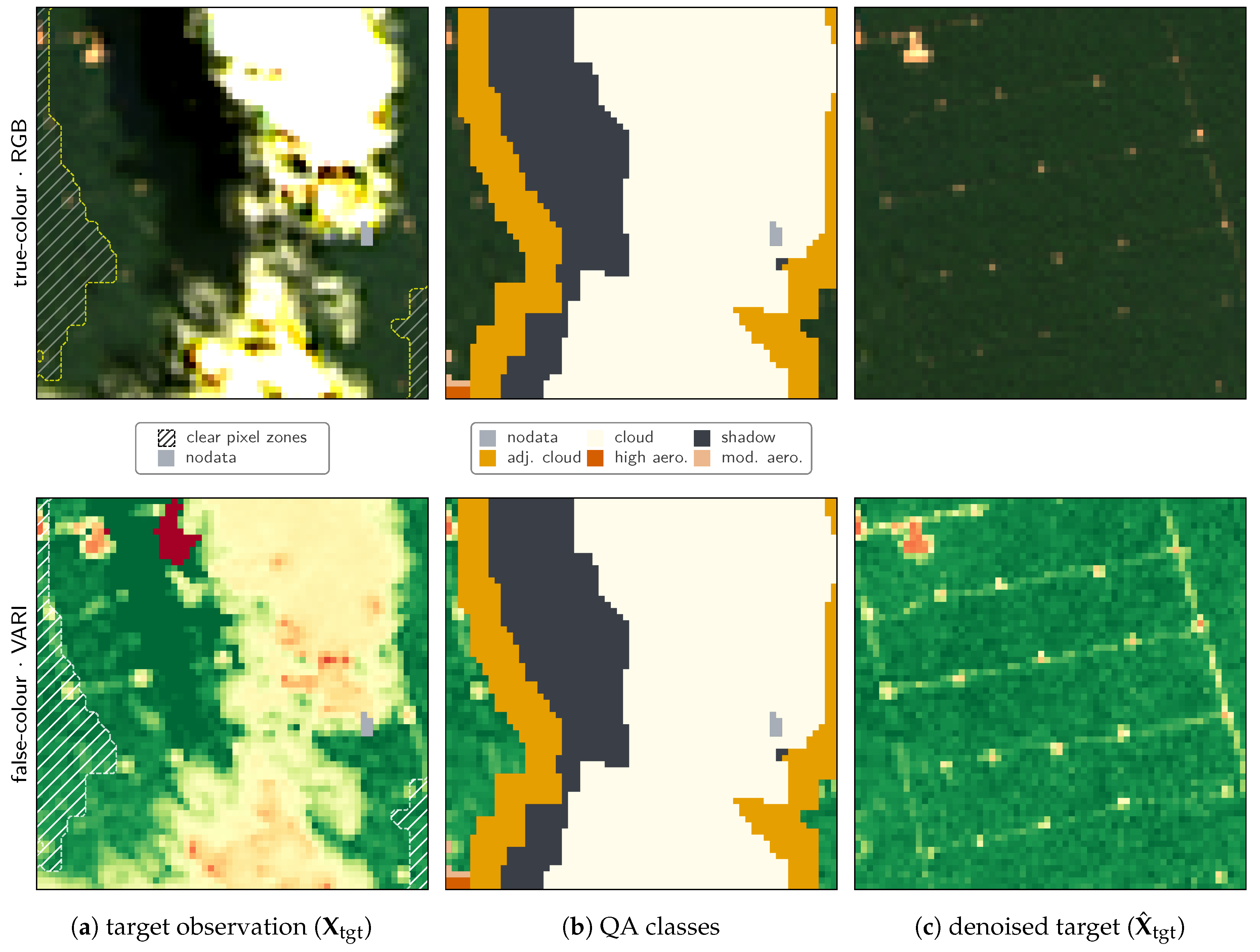
Given an observation whose surface is largely obscured, this stage reconstructs the cloud-free reflectance from the pixel’s surrounding temporal context (Figure 6); in effect, it denoises the scene of atmospheric occlusion. These reconstructions are what interpreters read to place the curated change dates of Section 3.5, and the encoder that produces them is the same one the downstream detector reads.
Figure 6.
Visual-interpretation panel: foundation-model reconstruction on a heavily clouded observation (one monitoring unit, single date; VARI vegetation index [18]). (a) The target observation, 90.2% masked; the dashed outline and faint hatch mark the clear-pixel zone — the small unmasked area which the identity bypass (Eq. 13) copies unchanged into the reconstruction. (b) The same frame’s Fmask-derived occlusion mask, coloured by class — cloud, cloud shadow, pixels adjacent to cloud, moderate and high aerosol, and no-data (invalid reflectance); cirrus, the mask’s remaining component, flags no pixel in this frame. (c) The denoised target. This monitoring unit holds a selective-logging feature that the cloud cover leaves entirely obscured in the observed frame.
Figure 6.
Visual-interpretation panel: foundation-model reconstruction on a heavily clouded observation (one monitoring unit, single date; VARI vegetation index [18]). (a) The target observation, 90.2% masked; the dashed outline and faint hatch mark the clear-pixel zone — the small unmasked area which the identity bypass (Eq. 13) copies unchanged into the reconstruction. (b) The same frame’s Fmask-derived occlusion mask, coloured by class — cloud, cloud shadow, pixels adjacent to cloud, moderate and high aerosol, and no-data (invalid reflectance); cirrus, the mask’s remaining component, flags no pixel in this frame. (c) The denoised target. This monitoring unit holds a selective-logging feature that the cloud cover leaves entirely obscured in the observed frame.
4.2. Downstream Soft-Label Regressor
For the downstream task, the pretrained encoder’s per-pixel representation of the target observation is read out and passed to a lightweight head that emits one scalar per target observation, covering the unit’s footprint: the downstream score (Figure 4b). The head takes the concatenation of the temporal and spatiotemporal embeddings (Eqs. 11–12), pools it over the grid, and maps it through a small multilayer perceptron to a scalar,
with the logistic function. The head is trained as a soft-label regressor against the continuous target of Section 3.5 (Eq. 9), by minimising the mean squared error
so the head learns the strength and recency of disturbance.
The samples in Eq. 16 are drawn from the 20 MUs and the 57 logging-free sites alike, but not symmetrically. Samples with come only from the 20 MUs: the logging-activity observations together with their clearest post-onset augmentations. For every such sample, the interval between the labelled event and the target observation is force-masked, so that post-disturbance observations never leak into the visible history. Samples with come from two disjoint sources. The first is within-MU: each MU contributes its own pre-disturbance observations, drawn round-robin from the pre-onset window over equal-count time bins crossed with cloud-fraction strata, so the baseline samples span the same temporal and atmospheric range as the set, at a one-to-one quota. Within that window, a warm-up withholds each MU’s first ten eligible observations after (Eq. 1) from the round-robin draw, so no baseline sample falls in the monitoring period’s opening stretch. The second is cross-MU: the 57 logging-free sites (Section 3.5) contribute negative samples at training time only, each counted toward a single MU’s quota. With augmentation included, the final dataset comprises 1,579 samples (807 with / 772 with ).
While the head trains, the encoder’s temporal blocks are frozen and only its spatial parameters are fine-tuned (Figure 4b), a split that keeps the label-free temporal representation intact while letting the spatial read-out adapt to the labelled task. The head is fed the visible input a deployed system actually sees (the raw observation with occluded pixels masked out) and is always given the real acquisition dates, so it cannot rely on a fixed temporal layout. Evaluation is by leave-one-MU-out cross-validation (CV) over the 20 MUs: each fold trains on the other 19, together with the training-only cross-MU negatives, and scores every observation of the held-out unit, so the pooled out-of-fold (OOF) predictions carry no cross-MU leakage.
4.3. Temporal Detection Rule
Applying the regressor to every HLS observation of a monitoring unit yields a score series ordered by acquisition date, which a temporal detector reads through two complementary filters. The early-detection (edge) filter responds to a sharp rise: at observation i it contrasts the mean score over the next f observations with the mean over the previous p,
and fires at the first i with , flagging an abrupt onset the moment it surfaces. The sustained-detection filter smooths the score with a length- Gaussian kernel g (standard deviation , normalised to unit sum) and adds a persistence requirement:
where centres the kernel and K is the number of consecutive observations that must stay above threshold, trading immediacy for robustness against transient spikes. The observations at which this criterion holds form the sustained detection zone; a run that stays above threshold for exactly K observations yields a zone of one observation, and every further above-threshold observation widens it by one. A monitoring unit fires when either filter fires. Each filter resolves two dates: a detection date at the first firing observation, where the disturbance first becomes recognisable, and a later confirmation date — the edge filter’s look-ahead endpoint ( observations on) or the end of the persistence run ( on) — at which the criterion is fully met and a warning could be published.
The seven filter parameters are fixed once, by an exhaustive grid search over the 20 MUs, rather than tuned per event. Every candidate configuration is scored on the per-MU confirmation lags (pooled) against a fixed lexicographic objective — first minimise early false positives, then the number of missed MUs, then the median confirmation lag — and the top-ranked configuration defines the reference operating point used throughout, four of whose values bound the filters’ reach: , , (a two-observation half-width), and . Of the three quantities that bound how far a filter reaches beyond its firing observation — the edge filter’s one-observation look-ahead (Eq. 17), the Gaussian kernel’s two-observation half-width, and the sustained filter’s four-observation persistence run (Eq. 18) — the persistence run is the widest and dominates. The corresponding backward margins, for the edge filter and the same two-observation half-width for the Gaussian kernel, are narrower still: too small to account for the ten-observation exclusion the training sampler applies at the start of a monitoring period (Section 4.2), which follows from its warm-up rather than either filter’s own reach. Because the selection depends only on the ordering of firings relative to each onset, and the same frozen score series feed every candidate, the search adds no free parameters to the regressor itself.
4.4. Implementation and Computing Environment
All experiments were run on a BDC-Lab instance — the geospatial data science computational environment of the Brazil Data Cube (BDC) initiative, hosted on the on-premises infrastructure of Brazil’s National Institute for Space Research (INPE) [54,55]. The instance runs Ubuntu 22.04 and provides a single NVIDIA H100 NVL GPU (94 GB), an AMD EPYC 9534 processor exposing 248 logical cores, and about 684 GiB of system memory. The models are implemented in PyTorch and trained in bfloat16 with graph compilation enabled, while the imagery corpora are assembled and read with an open geospatial stack (GDAL, xarray, zarr, and earthaccess). The foundation model totals 522,630 parameters; the downstream regressor’s head adds 33,281. In each cross-validation fold, only the head and the encoder’s spatial parameters are updated, 395,521 in all (Section 4.2). Exact layer widths, optimiser settings, the masking-curriculum schedule, and the detector grid are recorded in the released code.
Pretraining the foundation model took approximately 87 hours of active GPU time (about 3.6 days). The downstream regressor’s leave-one-MU-out cross-validation over the 20 MUs, with folds trained concurrently in batches of three on the same GPU, completed in 7.6 hours.
Assembling the foundation-model corpus (Section 3.4) — downloading, clipping to each monitoring unit, and converting to Zarr — shrank roughly 8 TB of raw HLS scenes to 53 GB of clipped tiles and, ultimately, to a 23 GB Zarr corpus. The downstream regressor’s candidate pool of all 254 selective-logging alerts (Section 3.5), processed the same way ahead of the 77-site selection, adds a further 15 GB of clipped tiles and 4.3 GB of Zarr data.
An AI code assistant hastened code development; all generated code was verified by the authors, who take full responsibility for the final results. A grammar assistant was also employed to check language inconsistencies.
5. Results and Discussion
5.1. Out-of-Fold Regression Accuracy
Pooled over the held-out observations (807 post-disturbance, 695 pre-disturbance), the regressor attains an OOF MSE of and an MAE of against the soft label v (Section 3.5), well below the of predicting the target mean and the of predicting zero — a reduction over the mean baseline (Table 2). The residual is larger on post-disturbance observations () than on pre-disturbance (), as expected for the harder rising and decaying portion of the target. Per-observation accuracy, however, is only a means to an end: what matters operationally is when the score first crosses a detection rule.
What carries the signal. The regressor operates on the raw observation a deployed system sees (with no manually engineered change index and no auxiliary inputs) and still resolves the disturbance: its score stays flat across the pre-disturbance window and rises sharply at the change. The pretrained spatiotemporal representation is what supplies the temporal context that makes this possible from a single visible input — the same context that lets the model reconstruct a clear surface through near-total cloud (Figure 6) and, in turn, guide the human interpretation behind the labels.
The per-fold error is not uniform (macro MSE ; Figure 7b): larger errors concentrate on MUs whose held-out observations are dominated by the rising and decaying portions of the target, consistent with the larger post-disturbance residual reported above. Two factors track this ranking. The amount of pre-onset monitoring history available to a fold is the strongest: MUs whose first observation falls closer to tend toward higher fold MSE (Spearman , ; Figure 7a), though MU12 runs against it: one of the longest pre-onset records (277 days) yet only a mid-ranked fold MSE. How long a fold trained before early stopping also tracks the ranking: folds reaching their best checkpoint after fewer epochs tend toward higher MSE (, ). The two predictors are not independent: longer-context folds also train longer ( between pre-onset span and epoch count), and a partial-correlation analysis points to context as the dominant factor — holding epoch count fixed, the span–MSE association stays strong (), whereas holding span fixed, the epoch–MSE association nearly vanishes ().
Training length as a trace, not a cause. The epoch pattern still admits a mechanical reading: under one shared early-stopping patience, applied uniformly to keep the folds comparable, the ten lowest-MSE folds reached their best checkpoint at a median of 112 epochs against 19 for the ten highest, and all ten highest stopped on the patience criterion while six of the ten lowest ran to the 120-epoch budget. A plausible, though untested, interpretation is that a flatter validation trajectory exhausts the common patience early, leaving the context-poor folds under-trained relative to their attainable error rather than genuinely converged; whether they would close the gap if trained well past the shared criterion is not tested here.
A candidate cause: contaminated context. Why should a short pre-onset window raise the error? Every model input is a target observation preceded by a lookback window of the previous 79 acquisitions, and when a unit’s onset falls early in its monitoring period that window reaches back before the period opens. Across the 20 units the onset target’s lookback crosses the start of the observations interval (the curated window) in 8, by as much as 77 acquisitions (roughly nine months of calendar time that no interpreter inspected for logging). Monitoring can begin partway through an extraction, so those earlier acquisitions may already carry logging that was never labelled; the observations meant to teach a clean baseline would then present a contaminated one, degrading the training target and the prediction together, and doing so for exactly the early-onset units that also hold the least context and the highest error. This cannot be confirmed here — any such events predate monitoring and were by construction never observed. It is also entangled with season: the two longest-lag units are the two shortest-context, highest-MSE folds, so both effects coincide at that extreme, though the context–MSE association survives dropping them (, ) with the mid-year onsets in between. The narrow takeaway is that the per-fold MSE spread (Figure 7b) should not be read as data difficulty alone, and separating genuine difficulty from boundary contamination (with monitoring periods opened well before onset) is left to future work.
5.2. Disturbance Specificity of the Score
A score that tracked the calendar rather than the canopy could reproduce a before-and-after contrast without detecting anything: it would only have to rise as each monitoring period ran on. The onsets rule this out. Across the 20 units the onset falls between 5 and 356 days after the unit’s first observation (Table S1), two of them within a fortnight of it and the rest between five and twelve months later. The 20 monitoring periods overlap in calendar time and the onset dates spread from January 2025 to January 2026, so on 215 of the 371 acquisition dates in the pooled record some units are already disturbed and others are not. Neither a calendar date nor a fixed offset from the opening of monitoring separates the pre- from the post-onset observations. Against that spread the out-of-fold score still splits cleanly: pooled across the 20 MUs, its mean is before the first logging activity and afterwards (medians and ), a five-fold jump (Figure 8a). The gap is highly significant — Welch’s , , with a large effect size [56] (Cohen’s ; a Mann–Whitney U test agrees) — so the elevated score is a response to the disturbance, not to the passage of time.
The pre-onset baseline is not a static landscape either. A monitoring unit is a fixed square (Section 3.2) rather than a delineation of the logging, so its record takes in the vegetation cycles and land-use change of the surrounding frontier (Section 3.4) under the heavy occlusion of the humid tropics. The 1,638 pre-onset observations pooled here cover all twelve months of the year, and the within-unit negatives that trained the regressor were drawn across the same time bins and cloud-fraction strata as the positive samples (Section 4.2), so the two sets are matched on date and viewing condition by construction. That variation left the pre-onset score at a median of zero. The comparison here is against ordinary landscape and atmospheric change, not against other disturbance types.
5.3. Near-Real-Time Detection
The two filters run together as a combination that encodes a single operating principle: detect as fast as the observations allow — when clear acquisitions, image quality, and the size of the cleared-area increment make an abrupt signal legible — and otherwise forgo immediate detection to secure a confirmation once the logging front has developed. For enforcement the confirmation date is the operative one: it is when a field team can be dispatched on an alert that has passed its persistence check, whereas the detection date is an earlier, internal indication.
At the confirmation operating point the detector confirms all 20 of 20 MUs on time, with 0 false positives and a median confirmation lag of days (Figure 9); most MUs are confirmed within about three weeks of the event, with a sparse long tail. The detection dates, the retroactive anchors of these confirmations, reach a median of days across the 19 of 20 that anchor after the onset. The remaining MU anchors two days early (the one false detection of Table 3), though its confirmation still fell after the onset.
Closing the temporal gap. The distribution is right-skewed: over half the units are confirmed within about two weeks, eighteen of the twenty within four months, and the two remaining only after 220 and 270 days. The elevated score responds to the disturbance, not to elapsed time: it jumps at the change from a flat, low baseline instead of climbing along a trend, the before-versus-after separation is large, and firing essentially never precedes the onset (Section 5.2). This is evidence that an HLS-based foundation-model pipeline can move selective-logging detection toward near-real-time operation, the intervention-facing capability a recent pantropical carbon synthesis sets apart from the slower carbon-accounting cycles and lists among the field’s needed improvements [4].
Seasonality of the confirmation lag. The long tail reflects viewing conditions rather than a failure to detect. A confirmation needs a cloud-free acquisition, and these concentrate in the dry season. Onsets in the dry season (August–November) are confirmed within about two weeks; an onset in the wet season is confirmed only once the clouds clear, which usually means waiting for the following dry season. The two January onsets, for instance, are not confirmed until 220 and 270 days later. Nineteen of the twenty confirmations fall in the same August–November window, regardless of when the onset occurred. Timeliness here is bounded by data availability, not by the score’s response to the disturbance.
Table 3 recasts these confirmations as a deliberately simplified binary test, centred on the decision the detector is designed to make: whether an alert precedes the documented onset. An observation counts as positive when it falls at or after ; the prediction is the detector’s firing state, at the detection date and at the confirmation date (Figure 8b,c). Specificity and precision carry the operational weight: one of the 1,638 pre-onset observations lies at or after the first firing at the detection date, and none at the confirmation date. Sensitivity is capped by construction: post-onset observations inside the detection-lag window count as false negatives, so its shortfall restates the lags of Figure 9, not a misclassification. Behaviour after the first alert is informative rather than targeted: once a unit is confirmed, later observations no longer change the alert.
The reference operating point emerges from the grid search of Section 4.3, not from hand-tuning. Sweeping each parameter about it, with the others fixed, shows how it is reached (Figure 10). Persistence K is the decisive control: raising it clears the last false alarms (three to none) and lifts on-time confirmations from 17 to all 20 MUs, at a cost of about eight days of median lag. The sustained threshold traces a valley — set too low, the smoother over-fires on score noise; set too high, it misses slow-rising events — and the reference sits at the widest false-alarm-free setting that still confirms every MU. The early threshold is likewise the lowest value at which the edge filter reaches full coverage without an early firing, and a minimum smoothing width suppresses the last noise-driven alarm. The reference point is therefore the corner of the search where zero false alarms and full coverage first coincide, not a latency-minimising choice: the sweeps show that spending a few false alarms buys only marginal reductions in lag.
Figure 11 traces this division of labour on two held-out units (MU3 confirmed by the edge filter, MU5 by the sustained filter), the two paths by which the combined rule detects as fast as the observations allow and otherwise waits for a confirmation once the logging front has developed.
Automation as an ally, not a replacement. In a critical operational setting the human interpreter must remain the final arbiter of an alert, and the results here are not an argument for removing that oversight but for relieving it. Screening a forest of continental extent by eye is precisely what makes selective logging so slow to catch, and the practical value of an early-warning tool grows as the manual burden it imposes shrinks. The semi-automatic monitoring advanced by Ortega Adarme et al. [31] and Chamorro Martinez et al. [32] adopts exactly this stance — a model disposes of the confident majority while interpreters concentrate on the ambiguous cases — and the pipeline developed here is complementary to it: the foundation model distils a year-long, cloud-ridden record over each monitoring unit into a short list of dated, confirmed candidates, and its cloud-penetrating reconstructions (Figure 6) already served, in this study, to guide the very interpreters who curated the labels. Read in this light, the contribution is a means to potentiate forest monitoring, directing scarce expert attention to the right place and time, rather than to supplant the expert.
From alert to field response. Trust in the alert stream is what turns detection into enforcement. Verifying an alert means sending a team into remote terrain, a scarce and costly resource; a false positive spends it on a non-event and, repeated, teaches teams to distrust the stream. The zero false positives recorded here therefore matter as much as the speed: they let a situation-room dashboard hand analysts alerts they can act on, concentrating limited enforcement capacity on the areas that most warrant it.
5.4. Broader Considerations
Label efficiency. A detector that confirms all 20 held-out events on time, with no false alarms, was obtained from just 1,579 labelled samples over 77 sites, with supervision from only 20 MUs. It reuses a representation pretrained without any labels on 91,145 samples from 1,404 sites — more than fifty times as much data — at no annotation cost. This backs the central claim that foundation models relax the annotation bottleneck that constrains conventional supervised approaches to a rare, hard-to-delineate disturbance class. This efficiency, however, does not follow from backbone generality alone. In the low-shot evaluations of AlphaEarth Foundations, Prithvi, a generalist backbone likewise pretrained on HLS, performed poorly when read through a minimal predictor, an outcome the evaluation itself attributes to a representation that requires further fine-tuning to transfer [21,23]. Just as telling, the construction of the small labelled set — within-MU negatives, clearest-target augmentation, and continuous soft-label targets — proved to matter as much as its size for transferring the pretrained representation.
Specificity across disturbance types. The pretraining corpus spans every DETER disturbance type, so the representation the detector reads was fitted on clear-cutting, degradation, mining, and fire alongside selective logging (Section 3.4). Supervision is narrower: it comes from selective-logging sites alone, and no observation of another disturbance type ever carries a label (Section 4.2). The expectation behind the broad corpus is that a representation exposed to the full range of frontier processes encodes what tells them apart, and that the head can read that distinction from the embedding — but nothing here tests it. The absence of false alarms is established on pre-onset windows of selective-logging units, which never probe how the score responds to a fire scar or a fresh mining pit. Whether the score is specific to selective logging among disturbance types, rather than to disturbance in general, is therefore open, and an ablation contrasting the present corpus against one restricted to selective logging would measure what the breadth buys.
Model sizing and planned ablations. The reported backbone is deliberately compact, at half a million parameters (Section 4.4). An earlier, larger configuration showed signs of overparameterisation relative to the available labelled signal, which motivated the narrower baseline. Controlled ablations that would quantify each design choice — representational capacity, the content-aware identity bypass, and global versus windowed spatial attention — are specified but not yet run, and are the most immediate next step. The present results should be read as the baseline those ablations are meant to probe, rather than as a tuned optimum.
Detection, not mapping. A more basic limitation is one of kind. This is a detection method, not a mapping one: it locates a disturbance in time but does not delineate its extent, and so estimates affected area poorly, unlike per-pixel mapping approaches such as that of Dalagnol et al. [16]. The tradeoff is deliberate: spatial detail is exchanged for the temporal detail an early-warning system most needs. Nor is it total: should the sustained detection zone’s area prove a usable proxy for disturbance severity, it would let alerts be ranked for the field triage above, a coarse stand-in for the spatial map this method forgoes.
Radar as a complement. The long confirmation tail above is a limit of the optical record, not of the score. Radar carries no such limit, and spaceborne L-band data now arrive fast enough to matter: NISAR, freely distributed, repeats exactly every 12 days [57] and releases products within 36–72 hours [58]; ALOS-4 repeats every 14 [59]. The transfer is not automatic. Per-pixel discrimination of selective logging has failed in both C- and L-band series, recovering breakpoints in at best half of the logged pixels [60]. NISAR’s own disturbance requirement is coarser still — one hectare, at least half the canopy lost, once a year [61]. But this method does not classify pixels. It scores an entire monitoring unit at once, and whether the clearings, skid trails, and log decks spread across that footprint shift its aggregate backscatter remains untested. The fine-grained alternative carries a price: Sentinel-1 radar shadow detects over 65% of disturbances above 200 m2, but confirms one only after about four months [62]. Fusion for coverage under cloud, not for finer sensitivity, is therefore a direction for future work.
Limitations. The labelled set is small and confined to a single biome; evaluation is MU-stratified, so it probes geographic generalisation, with the temporal confound controlled by the analysis of Section 5.2 rather than by an independent operational trial. A per-event operational validation over a larger sample of documented disturbances, comparing each alert against an independent reference date, is left to future work, as is transfer to other degradation processes (fire, edge effects) and to other biomes. Selective logging itself spans a range of impact: the same carbon synthesis reports markedly higher immediate carbon loss under conventional practices than under reduced-impact logging (mean versus of pre-disturbance stock) [4]. The detector presented here does not distinguish between these regimes, treating every selective-logging onset uniformly; separating them, and testing whether detection lag or score trajectory differs by intensity, is left to future work.
6. Conclusions
This work presented an innovative pipeline for near-real-time detection of selective logging in the Brazilian Legal Amazon that couples Harmonized Landsat–Sentinel-2 time series with a self-supervised spatiotemporal foundation model and a lightweight downstream detector. The foundation model, a compact masked autoencoder pretrained on 91,145 unlabelled samples from 1,404 monitoring sites, yields a per-pixel representation of forest dynamics. On that representation, a soft-label regressor trained on only 1,579 labelled samples (with supervision from just 20 MUs) reaches an out-of-fold MSE of 0.076 (-like 0.55) under leave-one-MU-out cross-validation.
Read by a lightweight temporal detector that pairs an edge filter with a persistence filter, this score confirms all 20 held-out logging events on time, with zero false positives and a median confirmation lag of days. That it stays flat and low across the pre-disturbance window and rises sharply only at the change, with a before-versus-after separation of and no confirmation before the known onset, points to genuine event detection rather than a calendar shortcut.
By learning from unlabelled HLS data, the approach eases the annotation burden that bottlenecks conventional methods, and the careful construction of the small labelled set proved decisive in reaching this performance. Its aim is not to displace the human interpreter who must sign off on an operational alert, but to concentrate that expertise where it is most needed — flagging when and where a disturbance has emerged across an area too vast to screen by eye. More broadly, the results show how geospatial foundation models can help close the temporal gap in forest-degradation monitoring, where the timeliness of an alert is as consequential as its accuracy. This speed comes at an accepted price: the method resolves disturbance in time rather than in space, and does not replace the area mapping of per-pixel approaches. For catching selective logging before its traces fade, trading spatial detail for temporal detail is a tradeoff worth making.
Immediate next steps are the controlled architecture ablations noted above, a larger-sample, per-event operational validation, and transfer to further degradation types and biomes. Beyond speed, the value at stake is temporal resolution on the disturbance itself. Because the detector already reads a continuous, per-observation score rather than a single onset flag, extending it to characterise how a disturbance evolves — not just when it starts — could support the shift from binary degradation classification toward the intensity continuum that recent carbon-synthesis work argues is needed to compare losses and gains across sites and forest types [4]. Transfer to other disturbance types carries a further benefit beyond broader coverage. Applied consistently across drivers, the same dense, per-observation timing that anchors selective-logging onsets here could resolve exactly when, how often, and in what order co-occurring disturbances unfold at a site, for instance, the drier microclimate and elevated fuel load that selective logging leaves behind, which raises the likelihood of subsequent fire [4]. Such precise sequencing is exactly what cumulative carbon-loss modelling needs to account for synergies between disturbances, rather than treating each as an isolated event.
Supplementary Materials
Table S1: per-monitoring-unit metadata (originating DETER identifier, out-of-fold regressor MSE, training epochs, documented onset, observations interval (the effective analysis window), detection/confirmation day, date, and sensor, and mean obstructed-pixel fraction over the confirmation window and over the whole monitoring unit) for all 20 monitoring units, sorted by MSE; Figure S1: detection mechanics for the same 20 monitoring units, in the style of Figure 11, four per landscape page across five pages, each reproducing the shared legend, followed by a sixth page with the covering caption; Equation S1: the standard confusion-matrix metric definitions used in Table 3. These items are provided in a single separate Supplementary Materials file.
Author Contributions
Conceptualization, E.T.; methodology, E.T.; software, E.T.; validation, E.T.; formal analysis, E.T.; investigation, E.T.; data curation, E.T., S.N. and D.B.; writing—original draft preparation, E.T.; writing—review and editing, E.T., G.M., S.N., D.B., G.Q. and L.A.; visualization, E.T.; supervision, G.Q. and L.A. All authors have read and agreed to the published version of the manuscript.
Funding
G.M. acknowledges funding from the São Paulo Research Foundation (FAPESP - grants 2025/07124-4 and 2025/28244-8). L.A. acknowledges funding from the National Council for Scientific and Technological Development - CNPq (310652/2025-1) and the UKRI Amazon-SOS (NE/X019039/1).
Data Availability Statement
The complete implementation — data-acquisition and preprocessing pipeline, foundation-model and detector training and inference code, and the trained model weights — is openly available at https://github.com/EvandroCT/mdpi-nrt-forest-monitoring. The datacube corpora and the trained weights are archived on Zenodo at https://doi.org/10.5281/zenodo.21712166. The underlying HLS v2.0 imagery and DETER warnings are public products of NASA and INPE, respectively.
Acknowledgments
The authors thank the Brazil Data Cube initiative and INPE’s Scientific Data Center (Centro de Dados Científicos) for the computing environment that made the experiments reported here possible.
Conflicts of Interest
The authors declare no conflicts of interest.
References
- Matricardi, E.A.T.; Skole, D.L.; Costa, O.B.; Pedlowski, M.A.; Samek, J.H.; Miguel, E.P. Long-term forest degradation surpasses deforestation in the Brazilian Amazon. Science 2020, 369, 1378–1382. [Google Scholar] [CrossRef] [PubMed]
- Lapola, D.M.; Pinho, P.; Barlow, J.; et al. The drivers and impacts of Amazon forest degradation. Science 2023, 379, eabp8622. [Google Scholar] [CrossRef] [PubMed]
- Pearson, T.R.H.; Brown, S.; Murray, L.; Sidman, G. Greenhouse gas emissions from tropical forest degradation: an underestimated source. Carbon Balance Manag. 2017, 12, 3. [Google Scholar] [CrossRef] [PubMed]
- Heinrich, V.; Holcomb, A.; Besnard, S.; Requena Suarez, D.; Cook-Patton, S.; Bourgoin, C.; Chazdon, R.; Gibbs, D.A.; Souza Mendes, F.; McNicol, I.; et al. A Meta-Analysis of Carbon Losses and Gains from Tropical Moist Forest Degradation and Regeneration. Sci. Adv. 2026, 12, eadz1923. [Google Scholar] [CrossRef] [PubMed]
- Mataveli, G.; Maure, L.A.; Sanchez, A.; Dutra, D.J.; de Oliveira, G.; Jones, M.W.; Amaral, C.; Artaxo, P.; Aragão, L.E.O.C. Forest Degradation Is Undermining Progress on Deforestation in the Amazon. Glob. Change Biol. 2025, 31, e70209. [Google Scholar] [CrossRef] [PubMed]
- Fearnside, P.M. Deforestation in Brazilian Amazonia: History, Rates, and Consequences. Conserv. Biol. 2005, 19, 680–688. [Google Scholar] [CrossRef]
- Asner, G.P.; Keller, M.; Pereira, R., Jr.; Zweede, J.C.; Silva, J.N.M. Canopy Damage and Recovery after Selective Logging in Amazonia: Field and Satellite Studies. Ecol. Appl. 2004, 14, S280–S298. [Google Scholar] [CrossRef]
- Taquary, E.C.; Nogueira, S.H.d.M.; Lopes, N.G.d.S.; Pereira, V.B.; dos Santos, L.B.; Barni, P.E.; de Aragão, L.E.O.e.C. Métrica da eficiência temporal na produção de avisos precoces de corte seletivo em sistemas de monitoramento florestal. In Proceedings of the Anais do Simpósio Brasileiro de Sensoriamento Remoto (SBSR), 2025. [Google Scholar]
- Diniz, C.G.; Souza, A.A.d.A.; Santos, D.C.; et al. DETER-B: The New Amazon Near Real-Time Deforestation Detection System. IEEE J. Sel. Top. Appl. Earth Obs. Remote Sens. 2015, 8, 3619–3628. [Google Scholar] [CrossRef]
- Dalagnol, R.; Phillips, O.L.; Gloor, E.; Galvão, L.S.; Wagner, F.H.; Locks, C.J.; Aragão, L.E.O.C. Quantifying Canopy Tree Loss and Gap Recovery in Tropical Forests under Low-Intensity Logging Using VHR Satellite Imagery and Airborne LiDAR. Remote Sens. 2019, 11, 817. [Google Scholar] [CrossRef]
- Brasil. Lei 9.605/1998: Brazilian Environmental Crimes Law Federal law establishing criminal and administrative sanctions for conduct harmful to the environment. 1998. Available online: https://www.planalto.gov.br/ccivil_03/leis/l9605.htm (accessed on 2026-07-24).
- Broadbent, E.N.; Zarin, D.J.; Asner, G.P.; Peña-Claros, M.; Cooper, A.; Littell, R. Recovery of Forest Structure and Spectral Properties after Selective Logging in Lowland Bolivia. Ecol. Appl. 2006, 16, 1148–1163. [Google Scholar] [CrossRef]
- Souza, C.; Barreto, P. An alternative approach for detecting and monitoring selectively logged forests in the Amazon. Int. J. Remote Sens. 2000, 21, 173–179. [Google Scholar] [CrossRef]
- Asner, G.P.; Knapp, D.E.; Broadbent, E.N.; Oliveira, P.J.C.; Keller, M.; Silva, J.N. Selective Logging in the Brazilian Amazon. Science 2005, 310, 480–482. [Google Scholar] [CrossRef] [PubMed]
- Bullock, E.L.; Woodcock, C.E.; Olofsson, P. Monitoring tropical forest degradation using spectral unmixing and Landsat time series analysis. Remote Sens. Environ. 2020, 238, 110968. [Google Scholar] [CrossRef]
- Dalagnol, R.; Wagner, F.H.; Galvão, L.S.; et al. Mapping tropical forest degradation with deep learning and Planet NICFI data. Remote Sens. Environ. 2023, 298, 113798. [Google Scholar] [CrossRef]
- Maretto, R.V.; Fonseca, L.M.G.; Jacobs, N.; Körting, T.S.; Bendini, H.N.; Parente, L.L. Spatio-Temporal Deep Learning Approach to Map Deforestation in Amazon Rainforest. IEEE Geosci. Remote Sens. Lett. 2021, 18, 771–775. [Google Scholar] [CrossRef]
- Gitelson, A.A.; Kaufman, Y.J.; Stark, R.; Rundquist, D. Novel Algorithms for Remote Estimation of Vegetation Fraction. Remote Sens. Environ. 2002, 80, 76–87. [Google Scholar] [CrossRef]
- Janowicz, K.; Gao, S.; McKenzie, G.; Hu, Y.; Bhaduri, B. GeoAI: spatially explicit artificial intelligence techniques for geographic knowledge discovery and beyond. Int. J. Geogr. Inf. Sci. 2020, 34, 625–636. [Google Scholar] [CrossRef]
- Janowicz, K.; Mai, G.; Huang, W.; Zhu, R.; Lao, N.; Cai, L. GeoFM: how will geo-foundation models reshape spatial data science and GeoAI? Int. J. Geogr. Inf. Sci. 2025, 39, 1849–1865. [Google Scholar] [CrossRef]
- Jakubik, J.; Roy, S.; Phillips, C.E.; Fraccaro, P.; Godwin, D.; Zadrozny, B.; Szwarcman, D.; et al. Foundation Models for Generalist Geospatial Artificial Intelligence. arXiv 2023, arXiv:2310.18660. [Google Scholar]
- Liu, C.; Huang, W.; Zhu, X.X. LandSegmenter: Towards a Flexible Foundation Model for Land Use and Land Cover Mapping. arXiv 2025, arXiv:2511.08156. [Google Scholar] [CrossRef]
- Brown, C.F.; Kazmierski, M.R.; Pasquarella, V.J.; Rucklidge, W.J.; Samsikova, M.; Zhang, C.; Shelhamer, E.; Lahera, E.; Wiles, O.; Ilyushchenko, S.; et al. AlphaEarth Foundations: An Embedding Field Model for Accurate and Efficient Global Mapping from Sparse Label Data. arXiv 2025, arXiv:2507.22291. [Google Scholar] [CrossRef]
- Ju, J.; Zhou, Q.; Freitag, B.; Roy, D.; Zhang, H.; Sridhar, M.; Mandel, J.; Arab, S.; Schmidt, G.L.; Crawford, C.; et al. The Harmonized Landsat and Sentinel-2 version 2.0 surface reflectance dataset. Remote Sens. Environ. 2025, 324, 114723. [Google Scholar] [CrossRef]
- He, K.; Chen, X.; Xie, S.; Li, Y.; Dollár, P.; Girshick, R. Masked Autoencoders Are Scalable Vision Learners. In Proceedings of the Proceedings of the IEEE/CVF Conference on Computer Vision and Pattern Recognition (CVPR), 2022; pp. 15979–15988. [Google Scholar]
- Instituto Nacional de Pesquisas Espaciais (INPE). PRODES — Amazon deforestation monitoring by satellite. 2024. Available online: http://terrabrasilis.dpi.inpe.br/en/home-page/ (accessed on 2026-06-30).
- Planet Labs, P.B.C. NICFI Satellite Data Program User Guide. 2024. Available online: https://assets.planet.com/docs/NICFI_User_Guide_EN.pdf (accessed on 2026-07-11).
- Norway’s International Climate and Forest Initiative. NICFI Satellite Data Program enters new phase Free public access to the Planet–NICFI mosaics ended. 2025. Available online: https://www.nicfi.no/2025/01/28/nicfi-satellite-data-program-enters-new-phase/ (accessed on 2026-06-26).
- Norway’s International Climate and Forest Initiative. Norway cancels procurement for the Tropical Forest Satellite Data Program Next-phase procurement cancelled 9 September 2025 after an upheld legal challenge. Available online: https://www.nicfi.no/2025/09/09/norway-cancels-procurement-for-tropical-forest-satellite-data-program/ (accessed on 2026-07-02).
- Sahbi, H. Label-frugal satellite image change detection with generative virtual exemplar learning. arXiv 2025, arXiv:2510.06926. [Google Scholar]
- Ortega Adarme, M.; Queiroz Feitosa, R.; Nigri Happ, P.; De Almeida, C.A.; Rodrigues Gomes, A. Evaluation of Deep Learning Techniques for Deforestation Detection in the Brazilian Amazon and Cerrado Biomes From Remote Sensing Imagery. Remote Sens. 2020, 12, 910. [Google Scholar] [CrossRef]
- Chamorro Martinez, J.A.; Ostwald Pedro da Costa, G.A.; Messias, C.G.; de Souza Soler, L.; de Almeida, C.A.; Queiroz Feitosa, R. Enhancing deforestation monitoring in the Brazilian Amazon: A semi-automatic approach leveraging uncertainty estimation. ISPRS J. Photogramm. Remote Sens. 2024, 210, 110–127. [Google Scholar] [CrossRef]
- NASA Land Processes Distributed Active Archive Center. Harmonized Landsat Sentinel-2 (HLS) Product User Guide, Version 2.0. 2026. Available online: https://lpdaac.usgs.gov/documents/1698/HLS_User_Guide_V2.pdf (accessed on 2026-06-26).
- NASA Goddard Space Flight Center. Harmonized Landsat Sentinel-2 (HLS). 2026. Available online: https://hls.gsfc.nasa.gov/ (accessed on 2026-07-07).
- European Space Agency. Copernicus Sentinel-2 mission update: transfer of duty from Sentinel-2A to Sentinel-2C on 21 January 2025. Available online: https://sentinels.copernicus.eu/-/copernicus-sentinel-2-mission-update-transfer-of-duty-from-sentinel-2a-to-sentinel-2c-on-21-january-2025 (accessed on 2026-06-26).
- Zhu, Z.; Woodcock, C.E. Object-based cloud and cloud shadow detection in Landsat imagery. Remote Sens. Environ. 2012, 118, 83–94. [Google Scholar] [CrossRef]
- Vermote, E.; Justice, C.; Claverie, M.; Franch, B. Preliminary analysis of the performance of the Landsat 8/OLI land surface reflectance product. Remote Sens. Environ. 2016, 185, 46–56. [Google Scholar] [CrossRef] [PubMed]
- Bommasani, R.; Hudson, D.A.; Adeli, E.; et al. On the Opportunities and Risks of Foundation Models. arXiv 2021, arXiv:2108.07258. [Google Scholar]
- Zhou, Z.H. A brief introduction to weakly supervised learning. Natl. Sci. Rev. 2018, 5, 44–53. [Google Scholar] [CrossRef]
- Radford, A.; Kim, J.W.; Hallacy, C.; Ramesh, A.; Goh, G.; Agarwal, S.; Sastry, G.; Askell, A.; et al. Learning Transferable Visual Models From Natural Language Supervision. In Proceedings of the International Conference on Machine Learning (ICML), 2021. [Google Scholar]
- Zhang, Z.; Zhao, T.; Guo, Y.; Yin, J. RS5M and GeoRSCLIP: A Large-Scale Vision-Language Dataset and a Large Vision-Language Model for Remote Sensing. IEEE Trans. Geosci. Remote Sens. 2024, 62, 1–23. [Google Scholar] [CrossRef]
- Dosovitskiy, A.; Beyer, L.; Kolesnikov, A.; Weissenborn, D.; Zhai, X.; Unterthiner, T.; Dehghani, M.; Minderer, M.; Heigold, G.; Gelly, S.; et al. An Image is Worth 16x16 Words: Transformers for Image Recognition at Scale. In Proceedings of the International Conference on Learning Representations (ICLR), 2021. [Google Scholar]
- Pathak, D.; Krähenbühl, P.; Donahue, J.; Darrell, T.; Efros, A.A. Context Encoders: Feature Learning by Inpainting. In Proceedings of the Proceedings of the IEEE Conference on Computer Vision and Pattern Recognition (CVPR), 2016; pp. 2536–2544. [Google Scholar]
- Feichtenhofer, C.; Fan, H.; Li, Y.; He, K. Masked Autoencoders As Spatiotemporal Learners. In Proceedings of the Advances in Neural Information Processing Systems (NeurIPS), 2022; Vol. 35. [Google Scholar]
- Tong, Z.; Song, Y.; Wang, J.; Wang, L. VideoMAE: Masked Autoencoders are Data-Efficient Learners for Self-Supervised Video Pre-Training. In Proceedings of the Advances in Neural Information Processing Systems (NeurIPS), 2022; Vol. 35. [Google Scholar]
- Cong, Y.; Khanna, S.; Meng, C.; Liu, P.; Rozi, E.; He, Y.; Burke, M.; Lobell, D.B.; Ermon, S. SatMAE: Pre-training Transformers for Temporal and Multi-Spectral Satellite Imagery. In Proceedings of the Advances in Neural Information Processing Systems (NeurIPS), 2022; Vol. 35. [Google Scholar]
- Szwarcman, D.; Roy, S.; Fraccaro, P.; Gíslason, Þ.E.; Blumenstiel, B.; Ghosal, R.; de Oliveira, P.H.; et al. Prithvi-EO-2.0: A Versatile Multi-Temporal Foundation Model for Earth Observation Applications. arXiv 2024, arXiv:2412.02732. [Google Scholar]
- Godwin, D.; Li, H.; Cecil, M.; Alemohammad, H. Seeing Through the Clouds: Cloud Gap Imputation with Prithvi Foundation Model. arXiv 2024, arXiv:2404.19609. [Google Scholar]
- Goh, E.; Yepremyan, A.; Wang, J.; Wilson, B. MAESSTRO: Masked Autoencoders for Sea Surface Temperature Reconstruction under Occlusion. Ocean Sci. 2024, 20, 1309–1323. [Google Scholar] [CrossRef]
- Instituto Brasileiro de Geografia e Estatística (IBGE). Legal Amazon Official territorial delimitation of the Brazilian Legal Amazon. 2021. Available online: https://www.ibge.gov.br/en/geosciences/environmental-information/geology/17927-legal-amazon.html.
- Leal Filho, W.; Dinis, M.A.P.; Canova, M.A.; Cataldi, M.; Costa, G.A.S.d.; Enrich-Prast, A.; Symeonakis, E.; Brearley, F.Q. Managing ecosystem services in the Brazilian Amazon: the influence of deforestation and forest degradation in the world’s largest rain forest. Geosci. Lett. 2025, 12, 24. [Google Scholar] [CrossRef]
- Assis, L.F.F.G.; Ferreira, K.R.; Vinhas, L.; Maurano, L.; Almeida, C.; Carvalho, A.; Rodrigues, J.; Maciel, A.; Camargo, C. TerraBrasilis: A Spatial Data Analytics Infrastructure for Large-Scale Thematic Mapping. ISPRS Int. J. Geo-Inf. 2019, 8, 513. [Google Scholar] [CrossRef]
- Loshchilov, I.; Hutter, F. SGDR: Stochastic Gradient Descent with Warm Restarts. In Proceedings of the International Conference on Learning Representations (ICLR), 2017. [Google Scholar]
- Ferreira, K.R.; Queiroz, G.R.; Vinhas, L.; Marujo, R.F.B.; Simoes, R.E.O.; Picoli, M.C.A.; Camara, G.; Cartaxo, R.; Gomes, V.C.F.; Santos, L.A.; et al. Earth Observation Data Cubes for Brazil: Requirements, Methodology and Products. Remote Sens. 2020, 12, 4033. [Google Scholar] [CrossRef]
- Brazil Data Cube Team; National Institute for Space Research (INPE). Brazil Data Cube Platform and BDC-Lab Data-Science Environment; National Institute for Space Research (INPE): Brazil, 2026; Available online: https://data.inpe.br/bdc/ (accessed on 2026-07-02).
- Cohen, J. Statistical Power Analysis for the Behavioral Sciences, 2nd ed.; Lawrence Erlbaum Associates: Hillsdale, NJ, USA, 1988. [Google Scholar] [CrossRef]
- NASA. NISAR Mission Overview. 2026. Available online: https://science.nasa.gov/mission/nisar/mission-overview/ (accessed on 2026-07-27).
- Alaska Satellite Facility. NISAR Data User Guide: Data Availability Level 1–3 products have a nominal latency of 36–72 hours. 2026. Available online: https://nisar-docs.asf.alaska.edu/availability-overview/ (accessed on 2026-07-28).
- ESA eoPortal. ALOS-4 (Advanced Land Observing Satellite-4). 2025. Available online: https://www.eoportal.org/satellite-missions/alos-4 (accessed on 2026-07-27).
- Hethcoat, M.G.; Carreiras, J.M.B.; Edwards, D.P.; Bryant, R.G.; Quegan, S. Detecting tropical selective logging with C-band SAR data may require a time series approach. Remote Sens. Environ. 2021, 259, 112411. [Google Scholar] [CrossRef]
- Chapman, B.; et al. The NASA ISRO SAR (NISAR) Mission – Validation of Science Measurement Requirements. In Proceedings of the IGARSS 2024 – 2024 IEEE International Geoscience and Remote Sensing Symposium, Athens, Greece, July 2024. [Google Scholar] [CrossRef]
- Welsink, A.J.; Dupuis, C.; Cue La Rosa, L.; Weghorst, M.; van der Zee, J.; van der Woude, S.; Peña-Claros, M.; Herold, M.; Fesenmyer, K.; Reiche, J. Monitoring fine-scale natural and logging-related tropical forest degradation using Sentinel-1. Remote Sens. Environ. 2025, 328, 114878. [Google Scholar] [CrossRef]
Figure 1.
Spatial pattern of selective logging in a 16 September 2025 observation. Under the Harmonized Landsat Sentinel-2 — a surface-reflectance product fusing Landsat and Sentinel-2 — the diagnostic skid trails (paths left by dragging felled logs), log landings (clearings where logs are collected for transport), and felling gaps (canopy openings left where trees were cut) span only a few 30 pixels, yet remain discernible.
Figure 1.
Spatial pattern of selective logging in a 16 September 2025 observation. Under the Harmonized Landsat Sentinel-2 — a surface-reflectance product fusing Landsat and Sentinel-2 — the diagnostic skid trails (paths left by dragging felled logs), log landings (clearings where logs are collected for transport), and felling gaps (canopy openings left where trees were cut) span only a few 30 pixels, yet remain discernible.
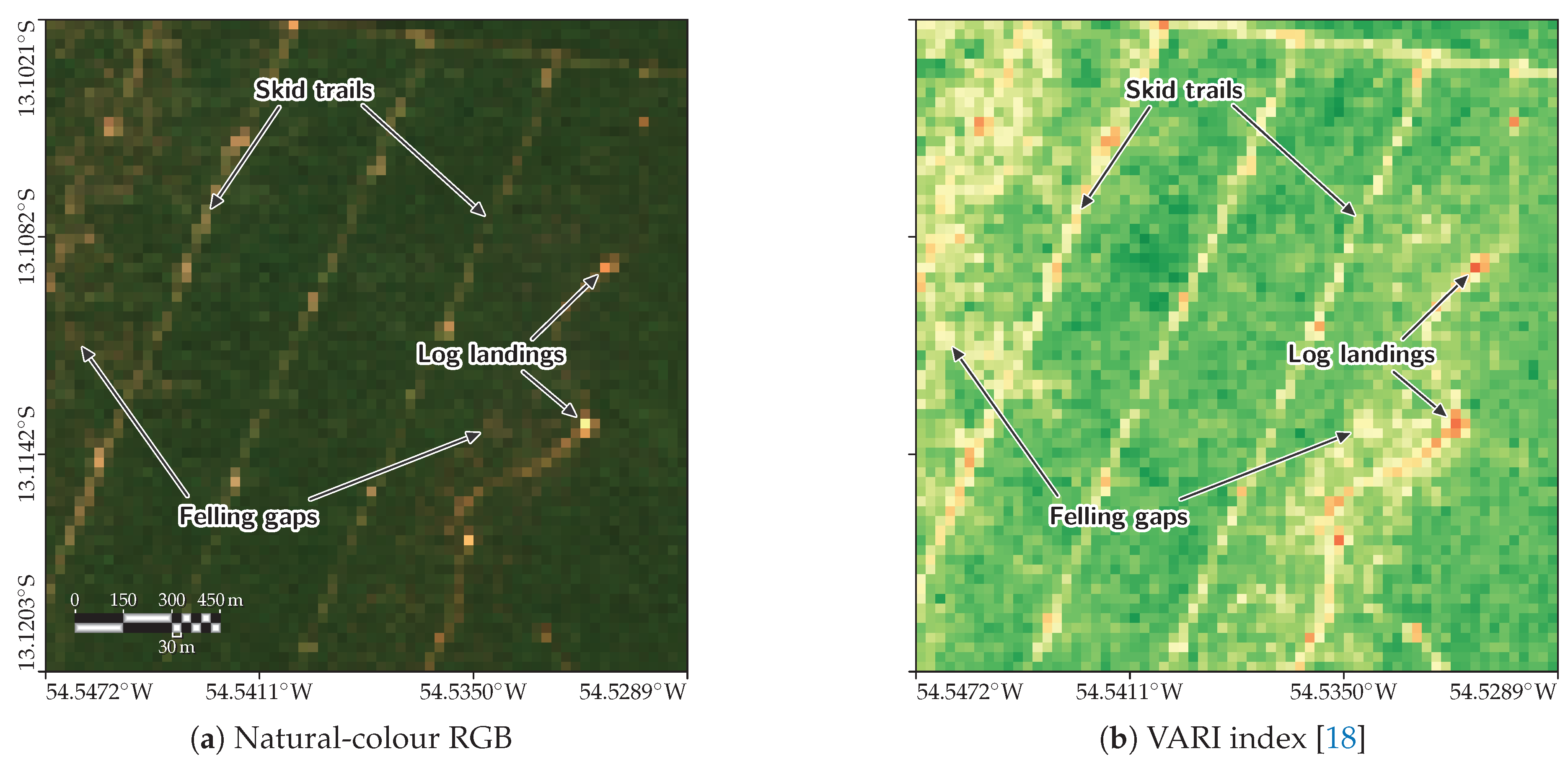
Figure 2.
Study area: monitoring sites over the Brazilian Legal Amazon (BLA; thick outline) and its states. In blue, the 1,404 foundation-model sites (clusters of one or more DETER alerts) used for self-supervised pretraining; in orange, the 77 labelled selective-logging sites used to train and evaluate the downstream regressor. Inset: location in South America.
Figure 2.
Study area: monitoring sites over the Brazilian Legal Amazon (BLA; thick outline) and its states. In blue, the 1,404 foundation-model sites (clusters of one or more DETER alerts) used for self-supervised pretraining; in orange, the 77 labelled selective-logging sites used to train and evaluate the downstream regressor. Inset: location in South America.
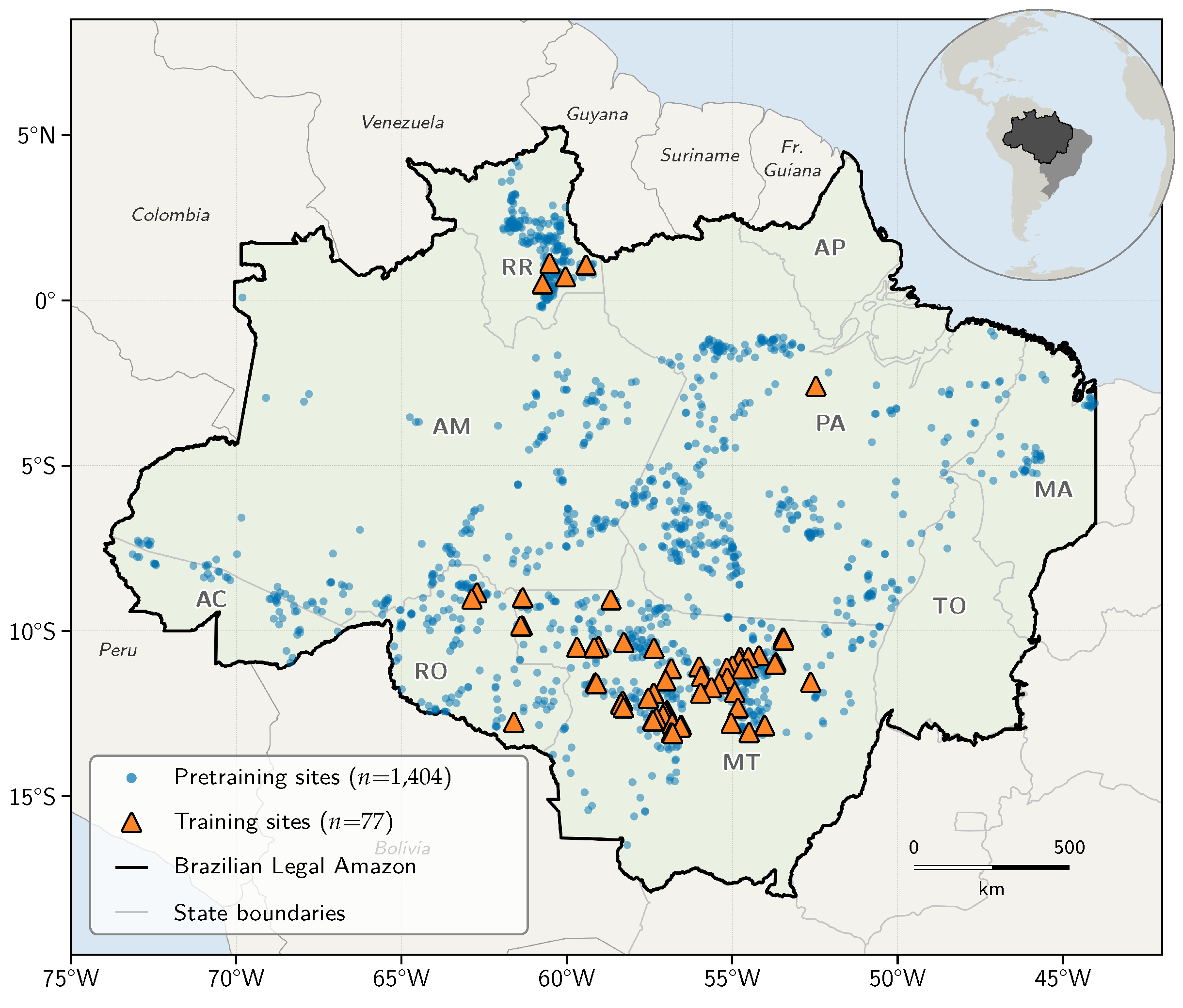
Figure 3.
Sampling relationship for one example cluster of six DETER alerts in Buriticupu, Maranhão: five Desmatamento CR (clear-cut deforestation) and one Degradação (degradation) alert, view dates 10–25 January 2026. The monitoring site (MS), tiled into monitoring-unit (MU) footprints, engulfs the six enlarged alert boxes. The polygons (in the pretraining-site colour of Figure 2) form three disjoint groups: a contiguous block of four plus outliers to the north and southeast. The tiling is independent of this arrangement: the upper-left MU intersects five of the six alerts, the central alert spans four MUs, and the upper-right MU contains only the tip of the southeastern outlier. As the foundation-model clustering spans all disturbance types, none of the six alerts is selective logging.
Figure 3.
Sampling relationship for one example cluster of six DETER alerts in Buriticupu, Maranhão: five Desmatamento CR (clear-cut deforestation) and one Degradação (degradation) alert, view dates 10–25 January 2026. The monitoring site (MS), tiled into monitoring-unit (MU) footprints, engulfs the six enlarged alert boxes. The polygons (in the pretraining-site colour of Figure 2) form three disjoint groups: a contiguous block of four plus outliers to the north and southeast. The tiling is independent of this arrangement: the upper-left MU intersects five of the six alerts, the central alert spans four MUs, and the upper-right MU contains only the tip of the southeastern outlier. As the foundation-model clustering spans all disturbance types, none of the six alerts is selective logging.
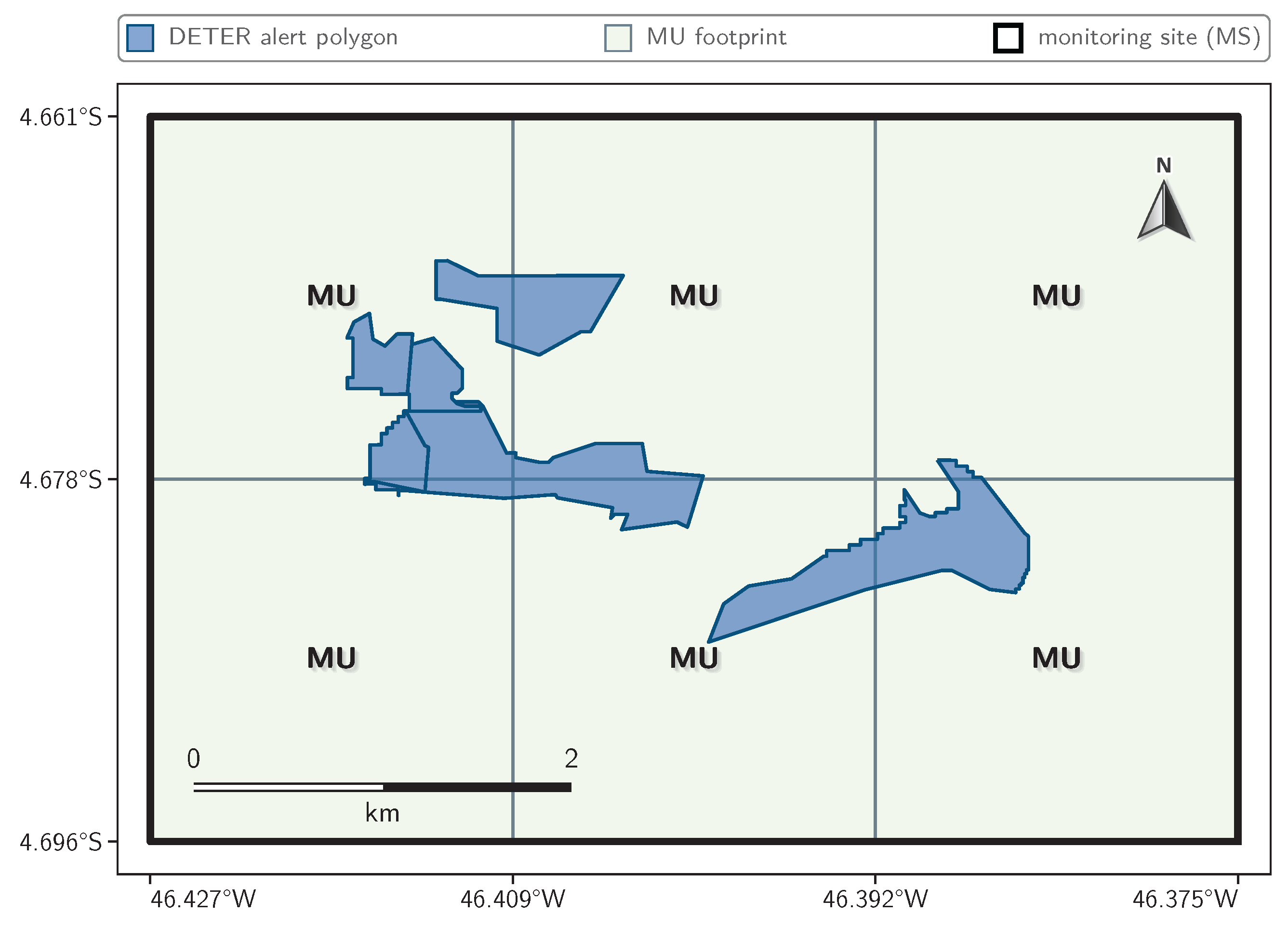
Figure 4.
Architecture of the two models; arrow shapes are , C the channel width at each stage, collapsing to once the target slot is selected from the input sample (Eq. 5; see legend). (a) The self-supervised foundation model: a spatiotemporal encoder — per-pixel temporal self-attention (Eq. 11) followed by global spatial self-attention (Eq. 12) — feeding a -convolution reconstruction decoder that recovers the denoised target via the visible-pixel identity bypass of Eq. 13. (b) The downstream model reuses the pretrained encoder — temporal frozen, spatial fine-tuned — and applies a lightweight trainable head — average pooling followed by a multilayer perceptron (MLP) — to the concatenated temporal and spatiotemporal embeddings to produce the downstream score (Eq. 15).
Figure 4.
Architecture of the two models; arrow shapes are , C the channel width at each stage, collapsing to once the target slot is selected from the input sample (Eq. 5; see legend). (a) The self-supervised foundation model: a spatiotemporal encoder — per-pixel temporal self-attention (Eq. 11) followed by global spatial self-attention (Eq. 12) — feeding a -convolution reconstruction decoder that recovers the denoised target via the visible-pixel identity bypass of Eq. 13. (b) The downstream model reuses the pretrained encoder — temporal frozen, spatial fine-tuned — and applies a lightweight trainable head — average pooling followed by a multilayer perceptron (MLP) — to the concatenated temporal and spatiotemporal embeddings to produce the downstream score (Eq. 15).
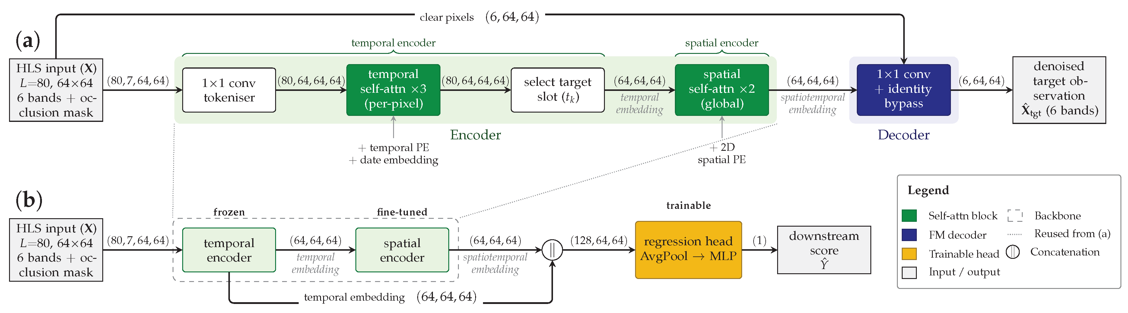
Figure 5.
Foundation-model learning curves. (a) Masked-reconstruction loss: per-step training (green) and per-epoch validation (red), log scale; the best validation loss is reached late in training (open circle), and both curves display a healthy entangled development. (b) Learning-rate schedule: cosine warm restarts (dotted guides, with their epochs ticked between the panels) cycle through the curriculum phases and continue through the extended mixed-regime training. (c) Band-gated masking curriculum, as the realised occlusion fraction per step: a staged advance from light to heavy masking (shaded) gives way to the full-range mixed regime. The surrounding shaded area is the standard deviation interval.
Figure 5.
Foundation-model learning curves. (a) Masked-reconstruction loss: per-step training (green) and per-epoch validation (red), log scale; the best validation loss is reached late in training (open circle), and both curves display a healthy entangled development. (b) Learning-rate schedule: cosine warm restarts (dotted guides, with their epochs ticked between the panels) cycle through the curriculum phases and continue through the extended mixed-regime training. (c) Band-gated masking curriculum, as the realised occlusion fraction per step: a staged advance from light to heavy masking (shaded) gives way to the full-range mixed regime. The surrounding shaded area is the standard deviation interval.
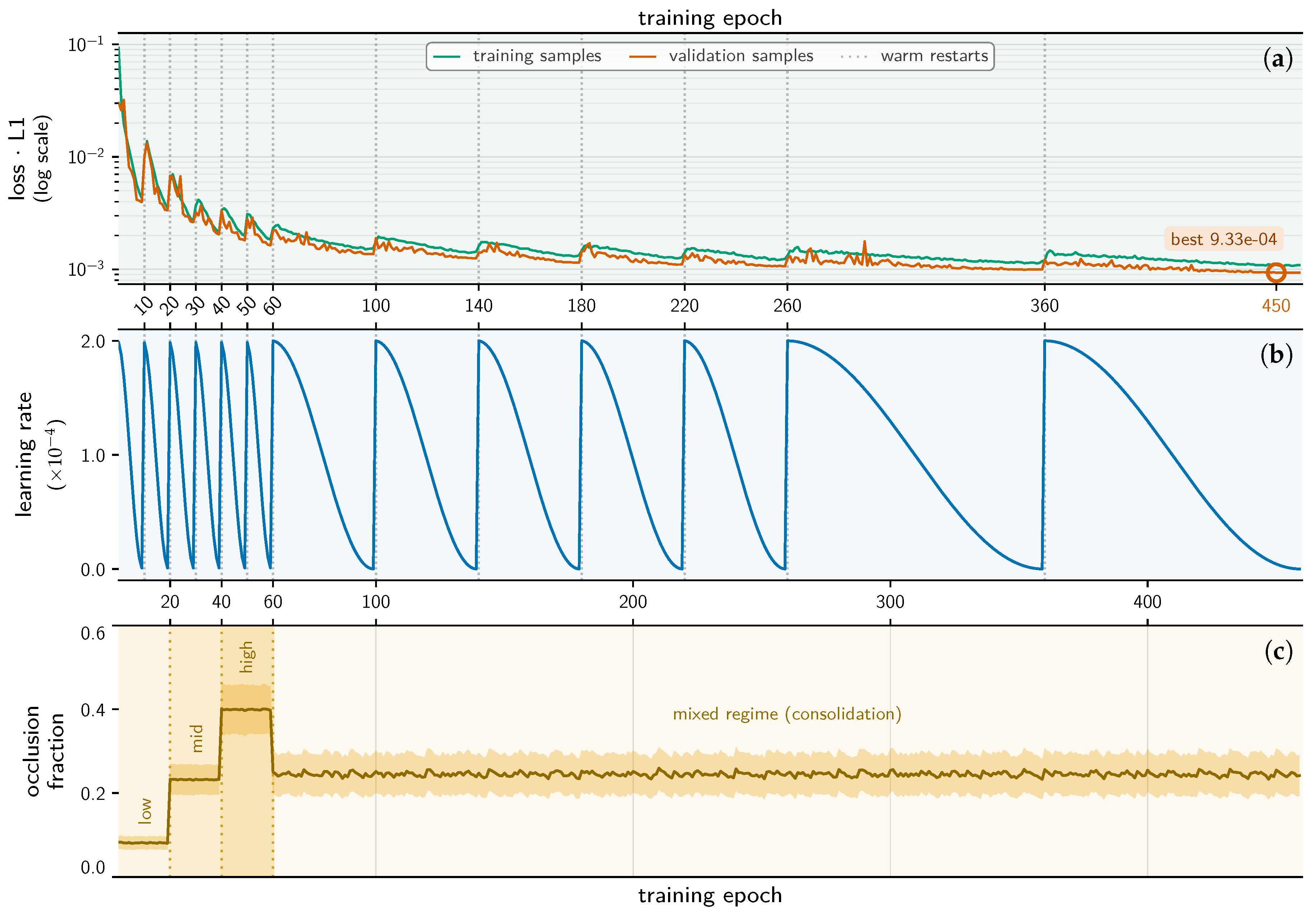
Figure 7.
Out-of-fold accuracy of the soft-label regressor under leave-one-MU-out cross-validation. (a) Score trajectories of the 20 held-out monitoring units as a ridgeline plot: one crest per MU, stacked top to bottom in ascending order of fold MSE (the order of panel (b) and Table S1), each tracing the unit’s out-of-fold — smoothed for display with a Nadaraya–Watson Gaussian kernel ( days) — over its -centred observations interval (days relative to , dash-dotted line), on the -day axis shared with Figure S1. Each crest spans only its unit’s observations interval, so its left edge marks how much monitoring history precedes ; the fill colour encodes the fold’s training length as epochs to its best checkpoint, read on the colour bar in panel (b) (– epochs). (b) Per-fold MSE for each of the 20 held-out monitoring units, sorted; the bars share panel (a)’s colour scale and order.
Figure 7.
Out-of-fold accuracy of the soft-label regressor under leave-one-MU-out cross-validation. (a) Score trajectories of the 20 held-out monitoring units as a ridgeline plot: one crest per MU, stacked top to bottom in ascending order of fold MSE (the order of panel (b) and Table S1), each tracing the unit’s out-of-fold — smoothed for display with a Nadaraya–Watson Gaussian kernel ( days) — over its -centred observations interval (days relative to , dash-dotted line), on the -day axis shared with Figure S1. Each crest spans only its unit’s observations interval, so its left edge marks how much monitoring history precedes ; the fill colour encodes the fold’s training length as epochs to its best checkpoint, read on the colour bar in panel (b) (– epochs). (b) Per-fold MSE for each of the 20 held-out monitoring units, sorted; the bars share panel (a)’s colour scale and order.
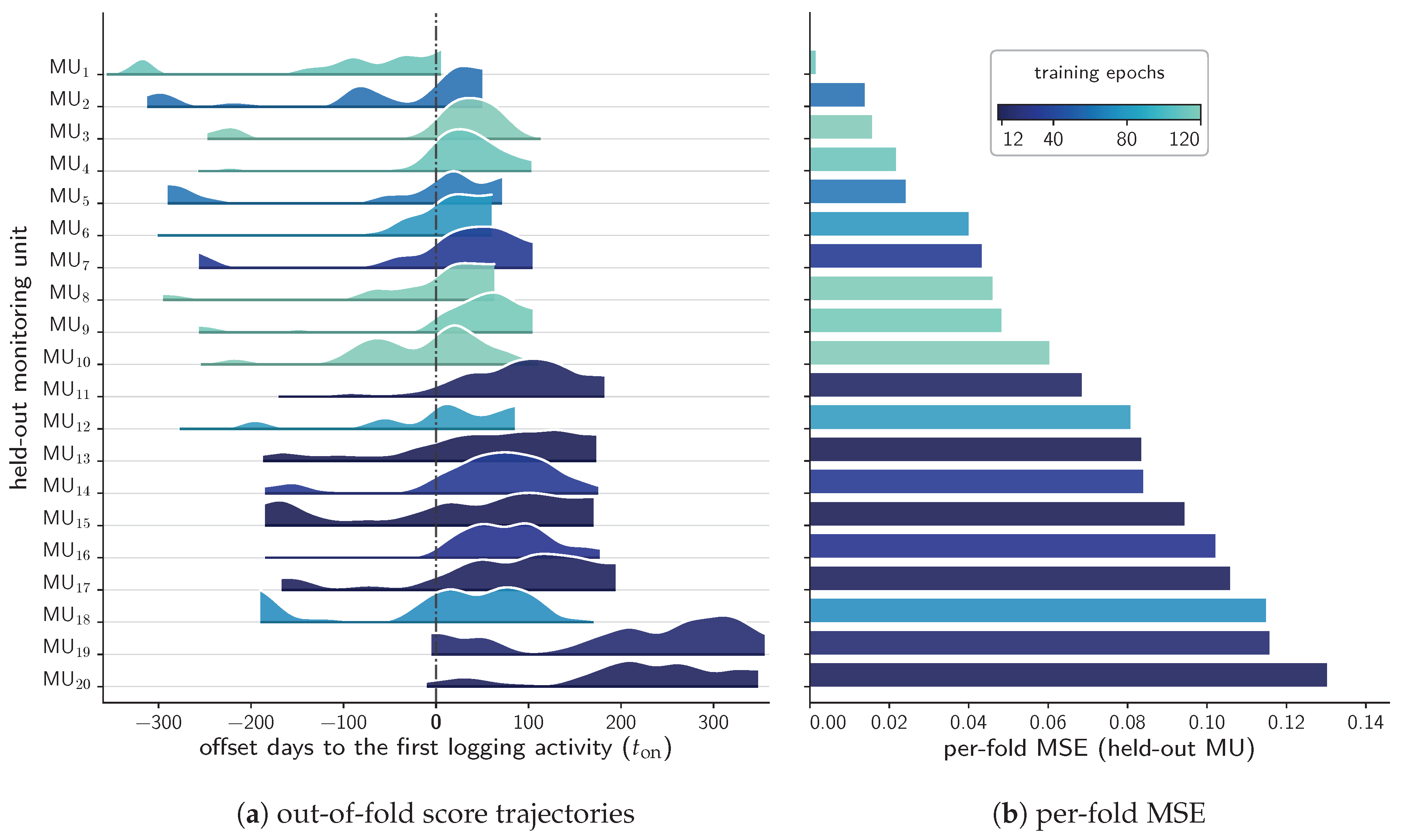
Figure 8.
Score separability and onset-centred confusion matrices. (a) Out-of-fold score before versus after the first logging activity , pooled over the 20 MUs (box: median and interquartile range; diamond: mean; points jittered). The score is near zero before and rises sharply after (, Welch’s t). (b,c) Confusion matrices (TN, true negative; FP, false positive; FN, false negative; TP, true positive; metric definitions in the Supplementary Materials) with ground truth centred on (an observation is positive if it falls at or after ) and the detector’s firing state as prediction, at the detection date (b) and the confirmation date (c). The false-negative cell is the detection-lag window (full battery in Table 3).
Figure 8.
Score separability and onset-centred confusion matrices. (a) Out-of-fold score before versus after the first logging activity , pooled over the 20 MUs (box: median and interquartile range; diamond: mean; points jittered). The score is near zero before and rises sharply after (, Welch’s t). (b,c) Confusion matrices (TN, true negative; FP, false positive; FN, false negative; TP, true positive; metric definitions in the Supplementary Materials) with ground truth centred on (an observation is positive if it falls at or after ) and the detector’s firing state as prediction, at the detection date (b) and the confirmation date (c). The false-negative cell is the detection-lag window (full battery in Table 3).
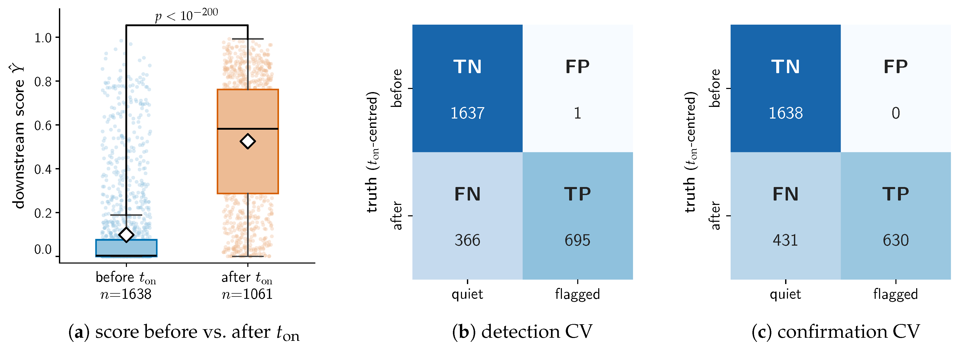
Figure 9.
Detection and confirmation lags of the reference detector over the 20 MUs. (a) Histogram of the per-MU detection lags (bins anchored at ). (b) Cumulative fraction of detections (first firing) and confirmations (alert-publishable) within a given lag of the first selective-logging activity . (c) Histogram of the per-MU confirmation lags. Dotted vertical lines mark the medians; the shaded region at lag is the false-positive zone.
Figure 9.
Detection and confirmation lags of the reference detector over the 20 MUs. (a) Histogram of the per-MU detection lags (bins anchored at ). (b) Cumulative fraction of detections (first firing) and confirmations (alert-publishable) within a given lag of the first selective-logging activity . (c) Histogram of the per-MU confirmation lags. Dotted vertical lines mark the medians; the shaded region at lag is the false-positive zone.
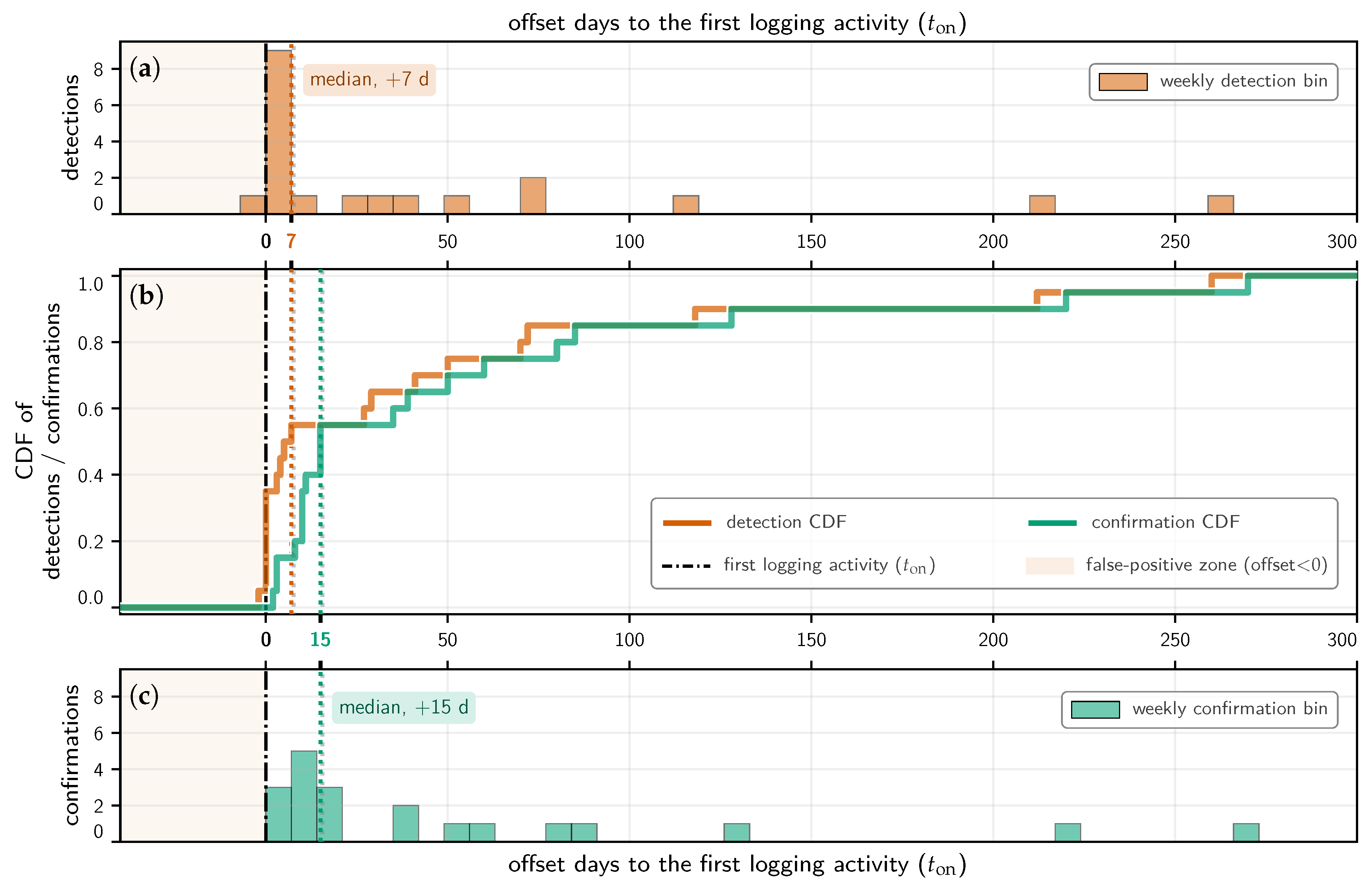
Figure 10.
One-dimensional sections through the detector grid search, each varying a single parameter about the reference operating point (grey band) with the others held fixed. Left axis: on-time confirmations (green) and early false alarms (red) over the 20 MUs; right axis: median confirmation lag in days (orange). The reference point is the setting at which false alarms reach zero while all 20 MUs are still confirmed.
Figure 10.
One-dimensional sections through the detector grid search, each varying a single parameter about the reference operating point (grey band) with the others held fixed. Left axis: on-time confirmations (green) and early false alarms (red) over the 20 MUs; right axis: median confirmation lag in days (orange). The reference point is the setting at which false alarms reach zero while all 20 MUs are still confirmed.
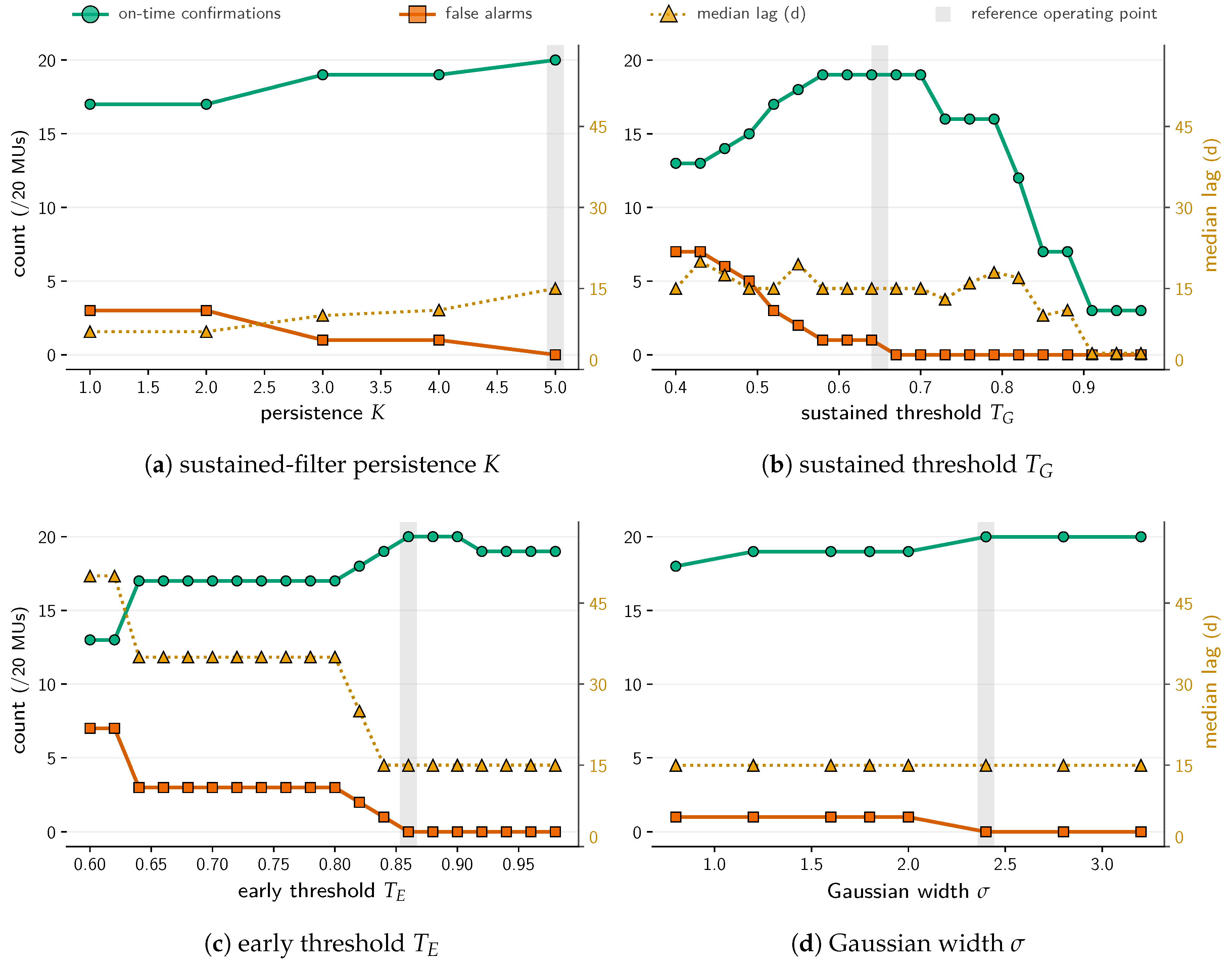
Figure 11.
Detection mechanics on two held-out MUs, with every plotted element named in the shared legend. (a) MU3, early-detection (edge) filter; (b) MU5, sustained-detection (Gaussian) filter. Each red column spans the four observations the edge kernel reads for its response peak (Eq. 17), two before it and one after; the axis is in days, so that fixed support widens where acquisitions are sparser. The shaded bands mark two edge-effect zones of different origin (Secs. Section 4.3 and Section 4.2).
Figure 11.
Detection mechanics on two held-out MUs, with every plotted element named in the shared legend. (a) MU3, early-detection (edge) filter; (b) MU5, sustained-detection (Gaussian) filter. Each red column spans the four observations the edge kernel reads for its response peak (Eq. 17), two before it and one after; the axis is in days, so that fixed support widens where acquisitions are sparser. The shaded bands mark two edge-effect zones of different origin (Secs. Section 4.3 and Section 4.2).
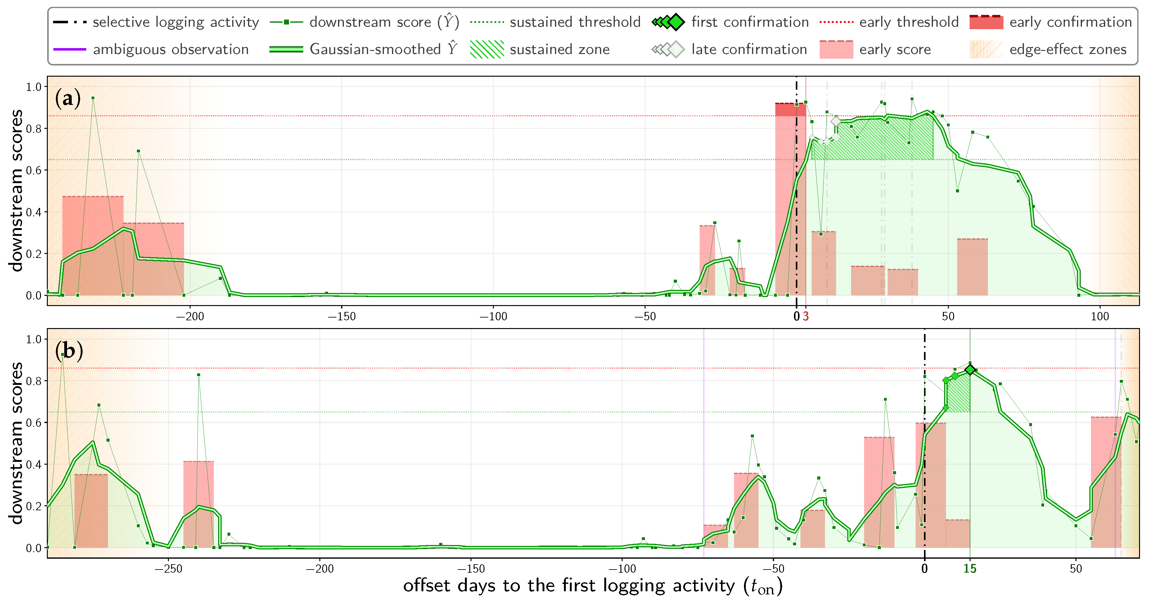

Table 1.
DETER alerts (1 January–1 May 2026) by disturbance type, and how many feed each model. Foundation-model pretraining uses all disturbance types — the 1,404 eligible monitoring sites (2,378 alerts) — whereas the downstream model uses only selective logging (77 out of the 254 alerts).
Table 1.
DETER alerts (1 January–1 May 2026) by disturbance type, and how many feed each model. Foundation-model pretraining uses all disturbance types — the 1,404 eligible monitoring sites (2,378 alerts) — whereas the downstream model uses only selective logging (77 out of the 254 alerts).
| disturbance type | alerts | pretraining | training |
|---|---|---|---|
| Deforestation | 2,348 | 1,657 | — |
| clear-cut | 2,266 | 1,590 | — |
| vegetation-loss | 82 | 67 | — |
| Degradation | 411 | 315 | — |
| Selective logging | 254 | 233 | 77 |
| geometric | 187 | 182 | 59 |
| disorderly | 67 | 51 | 18 |
| Mining | 199 | 126 | — |
| Fire scar | 76 | 47 | — |
| Total | 3,288 | 2,378 | 77 |
Table 2.
Out-of-fold regression error under leave-one-MU-out cross-validation (20 folds; held-out observations). The -like score is .
Table 2.
Out-of-fold regression error under leave-one-MU-out cross-validation (20 folds; held-out observations). The -like score is .
| Predictor | OOF MSE |
|---|---|
| Soft-label regressor | 0.076 |
| on post-disturbance | 0.105 |
| on pre-disturbance | 0.042 |
| Baseline: predict target mean | 0.168 |
| Baseline: predict zero | 0.324 |
Table 3.
Confusion-matrix summary with ground truth centred on the onset (an observation is positive if it falls at or after ; observations over the 20 MUs) and the detector’s firing state as the prediction, at the detection date and at the confirmation date. Sensitivity, specificity, precision, and follow their standard definitions (Supplementary Materials).
Table 3.
Confusion-matrix summary with ground truth centred on the onset (an observation is positive if it falls at or after ; observations over the 20 MUs) and the detector’s firing state as the prediction, at the detection date and at the confirmation date. Sensitivity, specificity, precision, and follow their standard definitions (Supplementary Materials).
| Operating point | TP | FP | TN | FN | Sens. | Spec. | Prec. | |
|---|---|---|---|---|---|---|---|---|
| Detection date | 695 | 1 | 1,637 | 366 | 0.655 | 0.999 | 0.999 | 0.791 |
| Confirmation date | 630 | 0 | 1,638 | 431 | 0.594 | 1.000 | 1.000 | 0.745 |
Disclaimer/Publisher’s Note: The statements, opinions and data contained in all publications are solely those of the individual author(s) and contributor(s) and not of MDPI and/or the editor(s). MDPI and/or the editor(s) disclaim responsibility for any injury to people or property resulting from any ideas, methods, instructions or products referred to in the content. |
© 2026 by the authors. Licensee MDPI, Basel, Switzerland. This article is an open access article distributed under the terms and conditions of the Creative Commons Attribution (CC BY) license (http://creativecommons.org/licenses/by/4.0/).
Copyright: This open access article is published under a Creative Commons CC BY 4.0 license, which permit the free download, distribution, and reuse, provided that the author and preprint are cited in any reuse.