
Submitted:
28 July 2026
Posted:
29 July 2026
You are already at the latest version
Abstract
Coupling-coordination scores are widely used to describe whether urban systems develop in step, although the usual index combines subsystem balance with average development level. This study separates these attributes for digital and transport infrastructure and relates them to urban environmental service performance in China. The analysis links city-level broadband use, mobile connectivity, data-center records, urban road provision, and seven municipal service indicators for 2002-2024. The preferred panel contains 6094 observations for 275 cities in 28 provinces. City fixed effects and province-by-year fixed effects absorb persistent local differences and common provincial shocks. After decomposing the conventional score, the standardized portfolio-level coefficient (0.188, p < 0.001) is more than four times the balance coefficient (0.045, p = 0.021). Balance remains positive before 2020 and when data-center capacity enters the digital index, but disappears with a road-density transport proxy. Component estimates locate the balance association in water and gas access, not sewage treatment, green coverage, or harmless waste treatment. The digital-transport interaction provides no evidence of superadditive returns. For SDG 9 and SDG 11 planning, infrastructure scale, relative balance, and external service outcomes should be monitored separately; synchronized construction alone does not establish environmental improvement.
Keywords:
coupling-coordination degree
; digital infrastructure
; transport infrastructure
; urban environmental services
; infrastructure portfolio
; city panel
; China
; sustainable cities
1. Introduction
Digital networks and transport systems increasingly share the same urban operating space. Freight platforms depend on roads, terminals, and reliable last-mile access. Intelligent traffic control depends on communication networks, data processing, and sensors. Water, waste, and emergency services use both digital information and physical routes. These connections join two parts of the 2030 Agenda. Sustainable Development Goal (SDG) 9 calls for reliable and sustainable infrastructure and wider access to information and communication technology, while SDG 11 links transport access, public services, environmental impact, and urban resilience [1,2,3]. The policy question is therefore not only how much infrastructure a city builds, but whether its infrastructure portfolio produces observable urban services.
Empirical research has taken a less integrated path. Studies of broadband and data infrastructure usually examine productivity, innovation, energy use, or carbon emissions [4,5,6,7,8,9,10,11]. Transport studies concentrate on market access, decentralization, induced travel, land conversion, and pollution [12,13,14,15,16,17,18,19]. A growing third literature constructs composite indices for two or more urban systems and evaluates their coupling-coordination degree (CCD). Digital economy and ecological quality, urbanization and the environment, green finance and digital development, or urban smartness and resilience are placed on a common scale; a rising CCD is then interpreted as evidence that the systems are becoming more coordinated and, often, more sustainable [20,21,22,23,24,25,26,27,28,29,30,31,32].
CCD compresses a complex relationship into a bounded number that is comparable across places and years and penalizes severe subsystem imbalance. Its label, however, invites a stronger interpretation than the formula supports. In the standard two-system formulation, the final score is the square root of the product of a coupling term and a weighted development term. A city can raise its CCD because the subsystems become more balanced, because both rise together, or because growth in one subsystem lifts the average despite continued imbalance. These routes imply different policy responses. Balance describes bottlenecks and relative configuration; the development term describes the scale of installed capacity. Their product does not directly measure cooperation, institutional integration, or environmental conversion.
This distinction matters in the case of digital and transport infrastructure. A balanced portfolio may reduce weak-link constraints: digital dispatch becomes more useful when roads are reliable, and physical connectivity becomes more productive when information can be transmitted and acted upon. At the same time, the environmental return from both systems depends on operating arrangements that their stocks do not measure. Broadband subscriptions and urban road area do not reveal whether agencies share data, whether maintenance is funded, whether traffic is priced, or whether treatment plants operate effectively. Two cities can post the same CCD while differing sharply in these institutional and operational conditions.
China provides a demanding setting in which to examine the issue. Digital connectivity and urban road provision expanded rapidly after 2000, but their sequencing varied among cities. Environmental services also improved, with large differences in water access, drainage, wastewater treatment, green space, and waste disposal. Previous work has often used provincial infrastructure variables to explain city outcomes or has treated a coupling score as the outcome to be described. Both choices limit inference. Province-level regressors cannot represent city-specific portfolio configurations, while a rising CCD does not establish that coordination improves an external sustainability outcome.
The present study changes both the measurement and the empirical design. Digital and transport infrastructure are measured at the city-year level. Digital capacity is represented by broadband users and mobile-phone users per resident, with licensed internet data-center stock added in a robustness test. Urban transport provision is represented by road area per capita, with road length per unit of built-up area used as an alternative. Within-year percentile ranks reduce sensitivity to changes in statistical units and preserve each city's relative position. These measures are matched to a seven-component index of municipal environmental services covering water, gas, drainage, sewage treatment, park green space, green coverage, and harmless waste treatment.
The empirical core separates the CCD into its pure coupling term, which captures relative balance, and its development term, which captures the average infrastructure level. The preferred model includes city fixed effects and province-by-year fixed effects. Identification therefore comes from changes in the relative infrastructure configuration of cities within the same province and year. Provincial economic cycles, regulations, infrastructure programs, price changes, and reporting shifts common to cities in that province-year are absorbed rather than approximated by a linear trend.
The conventional CCD has a positive coefficient of 0.205 under the preferred fixed effects, but decomposition changes its interpretation. A one-standard-deviation increase in portfolio level is associated with a 0.188-standard-deviation increase in the environmental-service index; the corresponding balance coefficient is 0.045. The balance estimate survives the addition of data-center stock and a pre-2020 restriction, weakens with a one-year lag, and disappears when transport is measured by road density instead of road area per resident. The robust empirical feature is the infrastructure-level association. Evidence for a separate balance association is smaller and specific to the service-availability definition of transport.
The component results sharpen the interpretation. Balance is positively associated with water and gas access, two network-access outcomes, but not with sewage treatment, drainage density, green coverage, park provision, or harmless waste treatment. The core environmental index, restricted to sewage, greening, and waste treatment, shows no balance effect. A separate interaction model provides no evidence of superadditive returns from simultaneous digital and transport expansion; its interaction coefficient is negative and marginal in the preferred specification. Fiscal-pressure splits and electricity-intensity regressions do not identify a convincing operating-burden or rebound mechanism.
This study contributes an external-outcome test of a familiar coordination indicator. Separating the coupling and development terms shows which part of the score is related to municipal services and prevents scale from being interpreted as balance. The 23-year city panel also avoids assigning one provincial infrastructure value to cities with different local portfolios. The resulting policy boundary is clear: balanced provision is associated with basic network access under the per-capita transport measure, but it does not replace the institutions, operating budgets, and sector-specific investments required for treatment and ecological outcomes.
Digital and transport infrastructures provide an informative test because they are general-purpose networks with different operational roles. Digital systems move information, while transport systems move people, equipment, and materials. Traffic control, field maintenance, emergency response, and municipal utility work require both. Their expansion can also diverge across cities, allowing balance to be separated empirically from the overall level of provision.
2. Literature Review and Analytical Framework
2.1. Digital Infrastructure and Urban Environmental Performance
Digital infrastructure can improve environmental performance through information, coordination, and organizational change. Broadband and mobile networks lower the cost of collecting and transmitting information [4,5,33]. Firms can monitor energy use, coordinate suppliers, and reorganize production. Municipal agencies can detect leaks, schedule waste collection, monitor treatment facilities, and publish environmental information. In this account, connectivity improves the productivity of existing physical assets rather than simply adding another asset class.
Evidence from China often supports this enabling view. Studies using the Broadband China program or city-level digital measures associate digital infrastructure with lower carbon emissions, improved carbon efficiency, green innovation, and eco-efficiency [6,7,8,9,20,21,22,23,34]. Proposed channels include industrial upgrading, innovation, service-sector development, resource reallocation, and stronger administrative monitoring. The size and sign of the estimated effects nevertheless differ by city size, industrial structure, human capital, and governance capacity. Digital access creates options, but local organizations determine whether those options are used for environmental purposes.
Recent research extends this discussion from environmental efficiency to urban resilience. Digital maturity can strengthen risk detection, information continuity, and emergency coordination, but its contribution depends on physical service systems and governance arrangements [35]. This dependence is especially relevant for municipal operations, where a digital warning, work order, or route plan has value only when a field team can reach the asset and complete the required intervention.
Digitalization also has a material footprint. Communication networks, terminals, data centers, cooling systems, and backup power consume energy and embodied materials. Lower information and transaction costs can expand online consumption, freight delivery, and device turnover. Efficiency gains may therefore coexist with scale and rebound effects [10,11]. Tang and Yang [10], for example, find higher emissions associated with digital infrastructure in Chinese cities over 2011-2019. The broader literature on digitalization and energy demand similarly warns that substitution effects need not dominate growth in activity [11].
Measurement is one reason findings diverge. A broadband-policy designation captures treatment timing but not installed capacity. Subscriptions combine network availability, affordability, demand, and user skills. Data-center licenses capture one infrastructure layer and are highly concentrated. Text-based policy attention measures government emphasis rather than physical stock. Composite digital-economy indices often mix infrastructure with industrial output and financial use, creating overlap with proposed mechanisms. This study focuses on access infrastructure and treats data-center stock as an extension rather than an interchangeable substitute.
2.2. Transport Infrastructure, Accessibility, and Environmental Services
Transport infrastructure alters the geography of economic activity. Roads and railways reduce travel costs, widen market access, and influence the location of firms and households. Research on China documents effects on industrialization, regional integration, and urban decentralization [14,15,16]. In cities, reliable roads can improve the routing of buses, waste vehicles, maintenance teams, and emergency services. Accessibility may also support consolidated freight and reduce the time required to deliver public services.
The same investments can increase environmental pressure. Added road capacity induces travel [12], and highway access can encourage suburbanization [13,15]. Lower access costs make peripheral development more attractive, lengthen trips, and expand the area requiring municipal networks. Roads also occupy land, fragment habitats, alter drainage, and create impervious surfaces [17,18]. Urban form mediates these outcomes: dense, mixed-use, transit-oriented development differs from dispersed road-led expansion [19,36].
Transport stock is therefore neither inherently green nor inherently harmful. Its effect depends on mode, location, utilization, pricing, and the surrounding land-use regime. Road area per capita is best read as an indicator of urban mobility provision, not as a measure of sustainable transport. That distinction is important for this paper. The research question is not whether roads are environmentally beneficial in isolation, but whether their configuration with digital access is associated with the operation of municipal environmental services.
Current sustainability research likewise treats infrastructure investment as a conversion problem rather than a stock count. Green-infrastructure investment can support urban resilience and sustainable development when finance, technology, and operating institutions connect the asset to a defined service outcome [37]. The same principle applies here: road provision can support installation, inspection, repair, collection, and emergency access, but it does not determine how those activities are funded or enforced.
2.3. Coupling-Coordination Measures and Their Interpretive Problem
Coupling-coordination analysis was introduced into urban and environmental studies to describe whether multiple systems evolve in a balanced way. Applications now span urbanization and ecological quality, digitalization and green development, infrastructure and resilience, and local development dimensions [24,25,26,27,28,29,30,31,32,38,39,40]. Recent articles in Sustainability apply the same family of measures to digital infrastructure and public employment services, provincial digital transformation and productivity, and the digital economy and environmental sustainability [38,39,40]. The standard procedure constructs a score for each subsystem, calculates a coupling term, combines the subsystem scores into a development index, and transforms their product.
The method is descriptive by construction. It does not observe a behavioral interaction, a production complementarity, or a causal effect. Li et al. [28] used a coupling model to track urbanization and environmental change, while Shen et al. [26] and Wang et al. [27] later identified sensitivity to subjective weights, formula choice, and compressed coupling values. Tomal [29] used CCD alongside convergence analysis, illustrating its usefulness for classification but not converting it into a causal parameter. Recent work continues to refine coupling formulas because traditional measures often cluster at high values or blur subsystem differences [30].
The most consequential issue for policy interpretation lies in the algebra. Let Digital_it and Transport_it be normalized city infrastructure scores bounded between zero and one. The conventional coupling term for two systems is:
reaches one when the scores are equal and declines as their relative difference grows. It is insensitive to common scale: two low-level but equal scores and two high-level but equal scores both have C = 1. The development term is:
The coupling-coordination degree is:
Equation (3) makes the interpretation clear. CCD is not a pure balance index. It rises with and . A positive regression coefficient on CCD may reflect balanced development, a higher average infrastructure level, or both. Because the two components have different policy levers, reporting only CCD can turn a measurement convenience into an overly broad claim about synergy.
The decomposition used here retains the familiar formula but estimates the environmental associations of and separately. This approach does not reject coupling analysis. It asks the narrower question required for policy: is environmental service performance associated with relative balance after the overall infrastructure level is held constant?
2.4. Portfolio Balance, Scale, and Environmental Conversion
The distinction between balance, level, and conversion also clarifies the connection to the SDGs. Portfolio level is closest to the infrastructure-access concerns in Targets 9.1 and 9.c. Balance describes the relative configuration of digital and transport provision, but no SDG target treats equality between sectoral indices as an outcome. Environmental conversion is tested against municipal services that overlap with the access, waste-management, and integrated-planning concerns of Targets 11.2, 11.6, and 11.b [1]. This mapping places CCD in its proper role: a descriptive portfolio measure that must be validated against external service outcomes.
The case for balance follows a weak-link argument. Digital and transport infrastructures perform distinct but complementary functions. Digital networks support traffic sensing, route optimization, asset registries, remote reporting, and work-order dispatch. Roads provide access for installing and repairing communication equipment and for crews that respond to digitally identified faults. In municipal services, information can improve monitoring and scheduling only when physical access permits action; field access becomes more productive when information identifies where and when intervention is needed [41,42]. A city that advances one system while neglecting the other may leave part of its installed capacity underused. This reciprocal service chain, rather than numerical similarity by itself, motivates the first expectation:
H1. Holding the average infrastructure level constant, a more balanced digital-transport portfolio is associated with stronger urban environmental service performance.
The infrastructure level has a separate effect. Higher digital access can support monitoring and coordination, while more road provision can improve access to network maintenance and public services. These direct capacity effects do not require the two systems to be equal or technologically superadditive. The development term should therefore be estimated rather than hidden inside CCD:
H2. A higher average level of digital and transport infrastructure is associated with stronger urban environmental service performance.
Balance and level need not carry equal weight across outcomes. Water and gas access are network-extension outcomes. Their improvement depends on connecting households and coordinating service delivery over space. Sewage and waste treatment are centralized or facility-dependent processes that require dedicated plants, collection and transfer systems, operating expenditure, compliance monitoring, and enforcement. Green coverage additionally depends on land allocation and ecological maintenance. Digital-transport balance may assist these activities, but it cannot replace sector-specific capital and governance. The expected pattern is therefore selective rather than uniform:
H3. The association with portfolio balance is stronger for network-access services than for treatment and ecological outcomes.
Coordination should not be equated with superadditivity. If digital and transport stocks are technological complements in the environmental-service production function, the marginal association of each should become more favorable as the other rises. Operational complementarity is a stronger condition than removing a weak link: it requires data use, field response, recurrent budgets, and sector-specific assets to work together. Rapid joint expansion can instead compete for fiscal and managerial attention, raise construction demand, and encourage additional travel or delivery. The product of standardized digital and transport levels is used as a diagnostic:
H4. Joint digital-transport expansion does not necessarily produce a positive interaction; superadditive environmental returns depend on operating and institutional conversion capacity.
3. Materials and Methods
3.1. Data Architecture and Unit of Analysis
The analysis combines three city-level sources. Municipal environmental services and urban roads come from the China City Construction Database, compiled from annual city construction statistics. The database records city administrative codes, environmental public services, land and built-up-area indicators, road provision, and related municipal infrastructure from 2002 through 2024. Digital access, socioeconomic controls, public finance, and licensed internet data-center records come from the city IDC database and its underlying statistical-yearbook panel. Electricity and industrial electricity measures for 2008-2019 are drawn from the raw China City Statistical Yearbook panel.
Administrative city codes are used as merge keys, with year and province code providing additional checks. Duplicate city-year records are removed before merging. No interpolated environmental outcome is used. Values outside plausible ranges are set to missing: percentages must lie between zero and 100, while counts, densities, areas, and populations must be nonnegative.
The merged data contain 6647 observations for 289 cities in 31 provincial-level regions. Regressions with a complete set of outcome, infrastructure, and control variables use 6094 observations for 275 cities in 28 provinces from 2002 to 2024. The panel is unbalanced. The reduction reflects control-variable availability rather than the assignment of provincial exposures; both focal infrastructure measures vary at the city-year level.
The city-level architecture resolves this measurement problem. Provincial backbones matter, but assigning the same infrastructure score to every city in a province makes it impossible to observe local portfolios and gives a provincial exposure the appearance of city-level variation. Here, broadband use, mobile use, road area, and data-center stock are attached to the city in which they are recorded. Province-by-year fixed effects can consequently absorb provincial infrastructure programs and macroeconomic conditions while leaving usable within-province city variation.
3.2. Urban Environmental Service Performance
The dependent variable summarizes seven municipal services: water access, gas access, drainage-pipe density in the built-up area, wastewater treatment, park green space per capita, green coverage of the built-up area, and harmless treatment of household waste. These indicators describe the provision and operation of environmental services experienced by urban residents. They do not cover the full domain of sustainability. Ambient pollution, greenhouse-gas emissions, ecosystem condition outside built-up areas, affordability, and within-city distribution remain outside the index.
Percentage variables are retained on their original scale after range checks. Drainage density and park green space per capita are transformed by ln(1 + x) to reduce the influence of highly skewed observations. Each component is winsorized at the first and ninety-ninth percentiles and standardized over the pooled sample. The index is the unweighted mean when at least five components are observed. Equal weights keep the construction transparent and prevent time-varying statistical weights from dominating the long panel.
Supplementary Table S1 reports the original unit, source, range check, transformation, and inclusion rule for each component and for all focal infrastructure measures. Water, gas, wastewater treatment, green coverage, and harmless waste treatment are recorded as percentages; drainage density is measured in kilometers per square kilometer of built-up area; and park green space is measured in square meters per resident.
A narrower core environmental index averages wastewater treatment, green coverage, and harmless waste treatment, requiring all three observations. This alternative excludes water and gas access. It tests whether a result for the broad index extends to services more directly connected with pollution treatment and ecological conditions.
3.3. City-Level Digital Infrastructure
The primary digital measure uses broadband access users and mobile-phone users per resident. The ratios are calculated from city counts and resident population. Both indicators combine installed access capacity with realized connection, an unavoidable feature of long city panels. They nevertheless remain closer to local network availability than policy designations or broad digital-economy indices.
The underlying statistical series change units or reporting conventions in some years. Applying a single pooled transformation would allow these breaks to alter intertemporal scale. The analysis therefore converts each indicator into a percentile rank among observed cities in the same year. The digital score is the mean of the broadband and mobile ranks. Within-year ranking preserves relative city position, bounds the measure between zero and one, reduces the influence of outliers, and prevents a national unit shift from generating a spurious time-series jump.
Licensed IDC stock is added to the digital score in a robustness test. IDC facilities capture a more computing-intensive layer of digital infrastructure but are concentrated in a minority of cities and may reflect licensing rather than continuously utilized capacity. They are not used to replace the broad access measure in the baseline.
3.4. City-Level Transport Infrastructure
The main transport measure is urban road area per capita, reported directly in the city construction statistics for 2002-2024. As with the digital indicators, it is converted to a within-year percentile rank. Road area per resident captures the provision of urban road space relative to the population served. It is not a measure of traffic, public-transport mode share, pavement quality, or regional highway access.
The alternative transport measure divides urban road length by built-up area and ranks the resulting density within year. Built-up-area data are consistently available through 2022, so this check uses a shorter panel. The two measures emphasize different aspects of transport provision: road area per capita concerns capacity relative to users, whereas road density concerns network intensity within the developed urban footprint.
3.5. Separating Portfolio Balance from Portfolio Level
The digital and transport percentile ranks enter Equations (1)-(3). The coupling term is the pure relative-balance measure. It approaches one as the ranks converge and falls when one system is far ahead of the other. The development term is their equal-weight average. Both terms are standardized before regression, allowing their coefficients to be compared in standard-deviation units.
The conventional CCD is retained as a benchmark. The analysis first estimates its association with environmental services, reproducing the interpretation available from a single coordination score. It then enters and separately. This decomposition is not an approximate statistical residualization; it follows the two components already embedded in the CCD formula.
Two additional diagnostics are reported. The absolute difference between the standardized digital and transport ranks provides a simple distance measure. The product of the standardized digital and transport scores captures whether joint high levels are associated with superadditive or diminishing returns after the main effects are included.
Figure 1 illustrates the measurement issue. For a fixed coupling value, CCD rises mechanically with the portfolio level. For a fixed level, it also rises with balance. A high CCD can therefore be produced by different configurations, and a change in CCD cannot be assigned to balance without examining its components.
, where C is pure portfolio balance and T is average infrastructure level. At any fixed value of C, a higher T mechanically raises CCD; the score therefore cannot identify a balance effect without holding level constant. Marker shapes distinguish the three level values in grayscale.
3.6. Control Variables
The preferred model includes six city-year controls. Economic development is represented by the city database's per-capita output measure. Openness captures the local importance of external trade. Industrial structure is measured by the service-sector share. Human capital reflects tertiary enrollment relative to population. Government intervention is based on general public budget expenditure relative to economic activity. Population density controls for the intensity of settlement and service demand. Continuous controls are winsorized and standardized.
The control set is limited to variables that precede or jointly shape infrastructure and environmental services. Municipal construction spending, environmental expenditure, and treatment capacity are not included in the baseline because they may be channels through which infrastructure portfolios are converted into service outcomes. Fiscal pressure, measured from the relation between budget expenditure and revenue, is used for a split-sample analysis rather than as a baseline control.
3.7. Econometric Specification
The preferred decomposition model is:
is the standardized environmental-service index for city i in province p and year t. is the standardized coupling or balance term, is the standardized portfolio level, and is the control vector. City fixed effects absorb time-invariant geography, administrative status, historical infrastructure, and persistent institutional differences. Province-by-year fixed effects absorb any shock shared by cities in the same province and year, including provincial programs, fiscal cycles, regulations, prices, disasters, and reporting conventions.
The coefficient compares changes in portfolio balance among cities operating under the same province-year environment while holding the average portfolio level constant. captures the association with infrastructure scale while holding balance constant. These are conditional associations, not causal treatment effects. Infrastructure placement and environmental services can respond to common city-specific shocks that the fixed effects and observed controls do not remove.
This fixed-effect combination removes time-invariant city heterogeneity and province-wide shocks in each year, including macroeconomic cycles and common provincial policies. It does not remove a city-specific investment program, urban expansion episode, or administrative reform that changes infrastructure and municipal services at the same time. The research design is therefore intended to estimate conditional empirical associations under demanding controls, not an exogenous treatment effect.
For comparison, a less demanding model replaces province-by-year effects with national year effects. The contrast shows how much the estimate depends on provincial variation. Standard errors are clustered by province, allowing arbitrary serial and cross-city correlation within provinces. With 28 clusters in the preferred sample, the covariance estimator uses a finite-sample correction and p-values use a Student-t reference with G - 1 degrees of freedom.
The interaction specification is:
is not used as a causal complementarity parameter. A positive estimate is consistent with increasing joint returns; a negative estimate is consistent with diminishing joint returns, congestion, rebound, or omitted conversion constraints. Its role is to test whether a high-high infrastructure configuration automatically carries an environmental premium.
3.8. Robustness, Component, and Constraint Tests
The decomposition is repeated with one-year-lagged balance and level, the core environmental outcome, an IDC-augmented digital score, road density in place of road area per capita, a pre-2020 sample, and a sample excluding the four centrally administered municipalities. These checks alter timing, measurement, outcome scope, and sample composition.
Each environmental component is then used as a separate dependent variable. This step is central to H3 because a broad index can conceal offsetting movements. Water and gas access are interpreted as network-access outcomes; sewage treatment, waste treatment, and greening reflect more sector-specific operating or ecological performance.
Two proposed mechanisms are examined with available data. The sample is split at the province-year median of fiscal pressure to determine whether the balance association is weaker where local budgets are more constrained. Electricity use per unit of GDP and industrial electricity use per unit of GDP are used as outcomes for 2008-2019 to assess an energy-demand channel. These tests are diagnostic. A subgroup coefficient difference is not treated as established without a direct interaction test, and an insignificant energy regression cannot rule out rebound in unobserved sectors.
4. Results
4.1. Descriptive Evidence
Table 1 summarizes the preferred complete-case sample. All focal indices retain substantial variation after city and province-year effects are considered. The digital and transport percentile measures have similar pooled dispersion by construction, while the pure coupling term is concentrated nearer its upper bound. This feature is common in traditional coupling measures and explains why formula choice can materially affect classifications [26,27,30].
The sample covers 275 cities for as many as 23 years, although missing controls and environmental components create an unbalanced panel. Broadband and mobile access rise strongly in raw units over the period, as does urban road provision. The ranking procedure does not use that common national increase for identification. Instead, it records whether a city moves relative to other cities observed in the same year.
The conventional CCD is positively correlated with both its balance and level components, but the relationship is much stronger with the level term. That correlation is mechanical as well as empirical: T_it appears directly in Equation (3). The regressions below determine whether the two components retain distinct associations after fixed effects and controls.
4.2. What the Conventional Coordination Score Contains
Table 2 compares the conventional score, the absolute gap, and the exact decomposition. With city and national year fixed effects, the CCD coefficient is 0.287 (p < 0.001). Replacing year effects with province-by-year effects reduces the estimate to 0.205, but it remains precisely estimated (p < 0.001). A standard coordination analysis could reasonably stop here and conclude that digital-transport coordination is associated with stronger urban environmental services.
That conclusion is incomplete. When CCD and the portfolio level enter together, the CCD coefficient declines to 0.155 in the preferred model. More importantly, the exact decomposition produces a balance coefficient of 0.045 (p = 0.021) and a level coefficient of 0.188 (p < 0.001). Because both variables are standardized, their magnitudes are comparable: the portfolio-level association is approximately 4.2 times the balance association.
The result supports H1 and H2, but not in equal measure. Relative balance has an association distinct from overall scale, yet most of the environmental-service gradient embedded in the conventional coordination score corresponds to the average infrastructure level. The simple absolute gap is insignificant. This contrast reflects the nonlinear and relative nature of the coupling term: penalizes a given absolute gap more strongly when the subsystem scores are low.
The decomposition also changes the policy reading. A city with a low average infrastructure level cannot compensate merely by keeping two weak systems equal. Conversely, expanding the lagging system may improve balance without producing a large change in environmental services unless the portfolio reaches a usable scale.
4.3. Main Estimates and Robustness
Table 3 reports balance and level estimates side by side. Under city and national year fixed effects, the balance coefficient is 0.051 (p = 0.040) and the level coefficient is 0.277 (p < 0.001). The preferred province-by-year model yields 0.045 and 0.188, respectively. Absorbing provincial shocks reduces both estimates but does not remove them.
Lagging the portfolio by one year weakens the balance coefficient to 0.037 (p = 0.078), while the level coefficient remains positive at 0.124 (p < 0.001). The difference suggests that the balance association is more contemporaneous or measured with less persistence than the capacity-level association. Reverse timing remains possible: cities extending water or gas networks may simultaneously adjust road and digital access.
Adding licensed IDC stock to the digital index produces a balance coefficient of 0.046 (p = 0.025) and a level coefficient of 0.157 (p < 0.001). The main pattern therefore does not depend on excluding data-processing capacity. Restricting the sample to 2002-2019 also leaves both coefficients positive: 0.049 for balance (p = 0.040) and 0.244 for level (p < 0.001). Excluding Beijing, Tianjin, Shanghai, and Chongqing has almost no effect on the preferred estimates.
The road-density test is the main qualification. When transport is measured by road length per unit of built-up area, the balance coefficient is -0.007 (p = 0.747), whereas the level coefficient remains positive at 0.059 (p = 0.018). Road area per resident and road density are not equivalent. The former captures capacity available to users; the latter captures the intensity of road layout in the urban footprint. The absence of a density-balance effect limits any claim that a single engineering ratio defines the relevant transport complement to digital access.
The denominator difference is consequential. Road area per resident and the two digital-access indicators are all scaled to the population served, so their balance describes relative service availability. Road density instead uses the built-up area, whose measured boundary changes as cities expand, and is available only through 2022. It describes network morphology rather than provision per user. The null result is not evidence against every form of digital-transport coordination, but it prevents the baseline estimate from being generalized to transport-network balance as a whole.
The core environmental outcome provides a second qualification. Balance has a coefficient of 0.015 (p = 0.434) when the dependent variable is restricted to sewage treatment, green coverage, and harmless waste treatment. The portfolio level remains positive at 0.070 (p = 0.024). Balance therefore contributes to the broad municipal-service index without showing a general relationship with treatment and ecological performance.
Figure 2 shows the asymmetry. Portfolio-level estimates are positive across every specification. Balance estimates are smaller and sensitive to timing, transport measurement, and outcome definition. The evidence supports a narrow association with per-capita service availability, not a general environmental return to balanced infrastructure.
4.4. Environmental-Service Components
Table 4 reports the component estimates and shows where the broad-index result originates. Portfolio balance is positively associated with water access (0.100, p = 0.003) and gas access (0.068, p = 0.002). Its coefficients for drainage density, sewage treatment, park green space per resident, green coverage, and harmless waste treatment are small and statistically indistinguishable from zero.
Portfolio level has a broader association. It is positive for water access (0.254, p < 0.001), gas access (0.181, p < 0.001), park green space per resident (0.253, p < 0.001), and green coverage (0.085, p = 0.003). The estimates for drainage density and harmless waste treatment are positive but imprecise, while sewage treatment remains insignificant.
These patterns support H3. Digital-transport balance is associated with services that require network extension to households. Water and gas systems rely on distributed connections, customer information, maintenance access, and reliable routing. Treatment outcomes depend more directly on plant capacity, operating standards, environmental enforcement, and continuous funding. Digital access and roads may facilitate those functions, but the estimates show no corresponding treatment or ecological effect.
The distinction also explains why the broad environmental-service index and the core environmental index give different answers. A composite outcome can be useful, but its label should not erase component content. In this sample, the balance coefficient describes access coordination more clearly than environmental treatment.
Figure 3 displays this division between access and treatment outcomes. The balance estimates for water and gas are distinct from the estimates for treatment and greening, whereas portfolio level has a broader but still non-uniform pattern.
4.5. Is Joint Expansion Superadditive?
Table 5 reports interaction estimates, which test a different proposition from balance. With city and national year fixed effects, the digital-transport product is negative but insignificant (-0.024, p = 0.216). In the preferred province-by-year model it becomes -0.029 and reaches only the 10% level (p = 0.099). The one-year-lagged estimate is -0.034 (p = 0.072). When IDC stock is added to the digital index, the interaction is more negative and statistically significant (-0.039, p = 0.010).
The alternative road-density interaction, the pre-2020 sample, and the exclusion of municipalities retain a negative sign but do not cross the 5% threshold. The core environmental outcome has an interaction coefficient near zero. Across these specifications, high digital and high transport provision shows no superadditive environmental return. The evidence is also too weak to establish a general negative interaction.
This is consistent with H4. Portfolio balance and portfolio level can each have positive associations even when the product of high levels does not. Balance concerns removal of relative bottlenecks. Level concerns available capacity. A positive interaction would require the marginal environmental productivity of one system to rise with the other. That stronger condition is not observed.
4.6. Fiscal Pressure and Energy-Demand Diagnostics
Table 6 reports the fiscal-pressure and energy-intensity diagnostics. The fiscal split does not support a simple operating-crowding-out mechanism. The balance coefficient is 0.047 (p = 0.051) in lower-pressure city-years and 0.068 (p = 0.018) in higher-pressure city-years. Portfolio-level coefficients are positive in both groups. Because the samples differ and no direct coefficient-equality test is reported, the larger high-pressure estimate should not be read as evidence that fiscal stress improves coordination returns. It does show that the baseline association is not confined to fiscally comfortable cities.
Electricity-intensity regressions are also inconclusive. Neither balance nor portfolio level is significantly associated with total or industrial electricity use per unit of GDP over 2008-2019. The estimates cannot verify the proposed rebound channel. They also cannot exclude energy effects outside the shorter electricity sample, changes in the power-generation mix, or energy embodied in construction.
These null diagnostics narrow the discussion. The paper does not attribute the component pattern to an empirically established fiscal or energy mechanism. The more defensible conclusion is that the observed balance association stops at basic access outcomes in this dataset. Identifying the organizational conversion process requires direct measures of environmental operating expenditure, interdepartmental data use, facility utilization, service quality, and enforcement.
5. Discussion
5.1. Coordination Is Not One Thing
The empirical findings expose a common ambiguity in coordination research. A positive CCD coefficient appears to validate the claim that synchronized systems improve sustainability. The decomposition shows that the claim contains at least two propositions: balanced systems perform better, and more developed systems perform better. Both receive some support here, but the level association is much larger and more robust.
This is not merely a statistical refinement. The policy instruments differ. Raising portfolio level may require expanding access, renewing facilities, or financing missing capacity. Improving balance may require directing marginal investment toward the lagging subsystem. Improving environmental conversion may require neither additional digital access nor more road area; it may require treatment facilities, maintenance staff, data-sharing protocols, pricing, and enforcement. A single score does not tell decision makers which margin is binding.
The result complements prior critiques of traditional CCD formulas [26,27]. Those studies emphasize subjectivity, compressed coupling values, and formula misuse. The present analysis adds an external-validity test. Rather than asking only whether a modified score produces plausible rankings, it asks whether the balance and level embedded in the score relate differently to an outcome outside the infrastructure pair. They do.
5.2. Why the Balance Association Appears in Access Services
Water and gas access share several characteristics. Both involve geographically distributed networks, customer connections, maintenance, billing information, and physical access for inspection and repair. Digital connectivity can support metering, reporting, and dispatch; roads can support installation and field service. A large imbalance between information access and physical mobility may leave one side of this service chain underused.
Sewage treatment, harmless waste treatment, and urban greening face a different production structure. Wastewater performance is bounded by sewer connections, treatment-plant capacity, energy and chemical inputs, discharge standards, and sustained operation. Waste treatment requires collection coverage, transfer facilities, landfill or incineration capacity, and compliance enforcement. Greening depends on land allocation, ecological design, irrigation, and maintenance. Digital systems can improve monitoring and roads can support logistics, but neither supplies the dedicated capital, operating budget, trained personnel, or enforcement authority that determines treatment performance. The insignificant balance coefficients for these outcomes therefore identify a production boundary rather than a failure of measurement alone.
This component pattern also speaks to the difference between smart and sustainable cities. Digital access can make a service system more observable and responsive without ensuring lower pollution or better ecological conditions [31,32]. The social-ecological-technological systems perspective treats technology as one layer of urban performance, not as an automatic substitute for institutions and ecosystems [30,31,32]. The findings fit that view: balance helps where coordination of access is central, but treatment outcomes require additional capacities.
5.3. Reading the Negative Interaction
The weakly negative digital-transport interaction should not be confused with the positive balance coefficient. A city can become more balanced by raising its lagging subsystem at a moderate level. The interaction asks whether already high levels reinforce one another in producing environmental services. The estimates offer no evidence that they do.
Several explanations remain plausible. Joint expansion may encounter diminishing returns after basic access is achieved. High-road, high-digital cities may also face more intense travel, delivery, construction, and land demand. Administrative attention can be devoted to network expansion while environmental operation catches up. Yet the fiscal and electricity tests do not establish these mechanisms, and the core environmental interaction is near zero. The safest reading is a boundary result: synchronized infrastructure construction should not be assumed to generate superadditive environmental returns.
5.4. Implications for Urban Infrastructure Planning
Bottleneck-led allocation. Cities should not treat equal digital and transport scores as a planning objective. In low-level cities, equal weakness is not coordination success. Investment should identify the service process that is failing, determine whether digital information or physical access is the binding constraint, and direct marginal resources to that constraint. A balance target is useful only when it removes a documented weak link.
Differentiate access from treatment. Water and gas access can benefit from integrated asset registries, work-order systems, mobile inspection, and route planning. Sewage, waste, and greening require a different priority order: dedicated treatment capacity, recurrent operating funds, qualified personnel, land, and environmental enforcement should be secured before digital or road additions are credited with a sustainability return. Project appraisal should name the responsible agency, operating budget, conversion pathway, and measurable service outcome.
Replace the single score with three-part monitoring. Infrastructure dashboards should report portfolio scale, relative balance, and external service performance separately. The same normalized subsystem scores can provide the first two measures, while sectoral indicators should track water and gas access, plant utilization, treatment compliance, collection coverage, service interruptions, and ecological quality. For transport authorities, digital integration should be assessed through changes in delay, empty mileage, maintenance response, service continuity, or pollution exposure, not through the joint growth of two investment categories.
5.5. Limitations and Research Agenda
Several limitations define the scope of the conclusions. The design is observational. City and province-by-year fixed effects absorb a large set of confounders, but city-specific time-varying shocks can still influence infrastructure and environmental services together. No policy discontinuity or external instrument isolates exogenous portfolio change. The estimates should therefore be interpreted as conditional within-city associations.
The timing test reinforces this caution. With a one-year lag, the balance coefficient falls from 0.045 to 0.037 and its p-value rises to 0.078. Urban expansion can generate broadband connections, roads, water pipes, and gas networks in the same construction cycle, especially in newly developed districts. Fixed effects do not remove this city-specific co-construction process. The estimates therefore cannot establish that a change in portfolio balance causes subsequent service expansion.
The digital measure uses realized broadband and mobile connections. These variables reflect both supply and demand, and they do not observe network speed, reliability, price, base-station density, cloud capacity, or public-sector interoperability. Within-year ranks address unit changes and outliers but sacrifice information about absolute national growth. A city can maintain the same rank while its physical access improves substantially.
The transport measure is also partial. Road area per resident does not describe public-transport quality, congestion, freight efficiency, walkability, or regional highway connectivity. Because the digital indicators and road area per resident all use a population denominator, the baseline balance term is best interpreted as alignment in service availability. Road density uses the changing built-up-area footprint and captures network layout; its balance coefficient is effectively zero. The result is therefore proxy-sensitive and should not be reported as a universal digital-transport balance effect. Future work should combine road topology, travel time, transit supply, logistics terminals, and traffic performance.
The environmental-service index is bounded. It captures municipal access, treatment, and greening, not emissions, air quality, water quality, biodiversity, climate resilience, affordability, or distribution within cities. Annual land-cover products could extend the analysis to impervious growth and ecosystem conversion [43], but they would still not observe service quality. The difference between the broad and core indices is a substantive finding, but it also shows why the term environmental sustainability must be used carefully.
Mechanism data are limited. Electricity intensity ends in 2019, and fiscal pressure is not the same as environmental operating expenditure. The available fiscal measure cannot isolate sewage-plant operation, waste collection, network maintenance, or environmental enforcement. The data also do not observe whether transport, utility, and environmental agencies share asset records or work orders. Table 6 should therefore be read as a set of diagnostic tests that fail to confirm two proposed channels, not as a complete mechanism analysis. Direct measures of maintenance, treatment-plant utilization, environmental staffing, earmarked operating expenditure, data-platform use, and interagency coordination would permit a more convincing test of conversion capacity. Firm- or project-level data could also reveal whether infrastructure complementarity operates through logistics, monitoring, or service delivery.
Finally, the coupling formula imposes equal weights on digital and transport systems. Equal weighting is transparent, but it is not an engineering estimate of optimal proportions. The relevant ratio likely differs by city size, density, geography, industrial structure, and service objective. Future research could estimate outcome-specific production frontiers or threshold relationships rather than assign a universal balance target.
6. Conclusions
Digital and transport infrastructures form a portfolio, but a single coordination score does not reveal which portfolio feature matters. In Chinese cities from 2002 to 2024, decomposition shows that average infrastructure level has a large and robust association with municipal environmental services. Relative balance has a smaller association concentrated in water and gas access and is not robust to the road-density transport measure.
The evidence distinguishes municipal access from environmental treatment. Balanced per-capita provision may ease network-access bottlenecks, but it does not predict sewage treatment, waste treatment, or urban greening. Simultaneous high-level expansion also shows no superadditive environmental return. Coordination in construction is not equivalent to coordination in operation, and neither guarantees environmental performance.
Urban planners can retain coupling measures as descriptive tools, provided that balance and level are reported separately and checked against external outcomes. The practical target should be a service-producing portfolio: sufficient capacity, attention to the lagging subsystem where it is genuinely binding, and explicit institutional arrangements that convert infrastructure into environmental operation. Without that final link, a city may improve its coordination score while leaving its most important environmental bottlenecks in place.
Supplementary Materials
The following supporting information can be downloaded at the website of this paper posted on Preprints.org, Table S1, variable definitions and data sources; Table S2, complete decomposition and robustness estimates; Table S3, component regressions; Table S4, fiscal-pressure and electricity-intensity diagnostics; and Python code used to construct the city panel, tables, and figures. The README records software requirements, source-data restrictions, and execution steps.
Author Contributions
Conceptualization, X.Z. and S.S.; methodology, S.S.; software, S.S.; validation, X.Z., S.S. and Y.Z.; formal analysis, S.S.; investigation, X.Z. and Y.Z.; resources, X.Z. and Y.Z.; data curation, S.S.; writing-original draft preparation, X.Z. and S.S.; writing-review and editing, X.Z., S.S. and Y.Z.; visualization, S.S.; supervision, X.Z.; project administration, X.Z.; funding acquisition, X.Z. All authors have read and agreed to the published version of the manuscript.
Funding
This research was funded by the Science and Technology Innovation and Demonstration Project of the Department of Transportation of Yunnan Province, "Research on the Development Strategy and Promotion Models of Highway-Related Economy in Zhaotong City" (Grant No. 2024-39).
Institutional Review Board Statement
Not applicable. This study uses secondary aggregate statistical data and does not involve human participants or animals.
Informed Consent Statement
Not applicable.
Data Availability Statement
The regression outputs, variable definitions, and replication code supporting the reported results are included in the supplementary materials. Restrictions apply to redistribution of some compiled source data. The underlying records are available from their respective statistical sources and data providers; the processed analytical dataset may be requested from the corresponding author subject to source-license conditions.
Conflicts of Interest
The authors declare no conflicts of interest. The funder had no role in the design of the study; in the collection, analysis, or interpretation of data; in the writing of the manuscript; or in the decision to publish the results.
Acknowledgments
The authors thank the statistical agencies and data providers whose records made the long city panel possible. During preparation of this manuscript, the authors used OpenAI Codex for statistical code review and language editing. The authors reviewed and edited the output and take full responsibility for the content of this publication.
References
- United Nations. Transforming Our World: The 2030 Agenda for Sustainable Development; United Nations: New York, NY, USA, 2015. [Google Scholar]
- OECD. Integrated Urban Policy to Achieve the SDGs. In OECD Regional Development Papers; OECD Publishing: Paris, France, 2025; Volume No. 179. [Google Scholar] [CrossRef]
- World Bank; Development Research Center of the State Council; P.R. China. Urban China: Toward Efficient, Inclusive, and Sustainable Urbanization; World Bank: Washington, DC, USA, 2014. [Google Scholar]
- Goldfarb, A.; Tucker, C. Digital economics. J. Econ. Lit. 2019, 57, 3–43. [Google Scholar] [CrossRef]
- Hjort, J.; Poulsen, J. The arrival of fast Internet and employment in Africa. Am. Econ. Rev. 2019, 109, 1032–1079. [Google Scholar] [CrossRef]
- Liao, K.; Liu, J. Digital infrastructure empowerment and urban carbon emissions: Evidence from China. Telecommun. Policy 2024, 48, 102764. [Google Scholar] [CrossRef]
- Wei, M.; Yin, X. Broadband infrastructure and urban carbon emissions: Quasi-experimental evidence from China. Urban Clim. 2024, 54, 101863. [Google Scholar] [CrossRef]
- Xiao, X.; Liu, C.; Li, S. How digital infrastructure construction affects urban carbon emissions: A quasi-natural experiment from the Broadband China policy. Sci. Total Environ. 2024, 912, 169284. [Google Scholar] [CrossRef] [PubMed]
- Ren, H.; Zhou, J.; Yu, Y.; Ye, M. Carbon emission reduction effects of digital infrastructure construction development: The Broadband China strategy as a quasi-natural experiment. Front. Environ. Sci. 2025, 13, 1510118. [Google Scholar] [CrossRef]
- Tang, K.; Yang, G. Does digital infrastructure cut carbon emissions in Chinese cities? Sustain. Prod. Consum. 2023, 35, 431–443. [Google Scholar] [CrossRef]
- Lange, S.; Pohl, J.; Santarius, T. Digitalization and energy consumption: Does ICT reduce energy demand? Ecol. Econ. 2020, 176, 106760. [Google Scholar] [CrossRef]
- Duranton, G.; Turner, M.A. Urban growth and transportation. Rev. Econ. Stud. 2012, 79, 1407–1440. [Google Scholar] [CrossRef]
- Baum-Snow, N. Did highways cause suburbanization? Q. J. Econ. 2007, 122, 775–805. [Google Scholar] [CrossRef]
- Faber, B. Trade integration, market size, and industrialization: Evidence from China's National Trunk Highway System. Rev. Econ. Stud. 2014, 81, 1046–1070. [Google Scholar] [CrossRef]
- Baum-Snow, N.; Brandt, L.; Henderson, J.V.; Turner, M.A.; Zhang, Q. Roads, railroads, and decentralization of Chinese cities. Rev. Econ. Stat. 2017, 99, 435–448. [Google Scholar] [CrossRef]
- Banerjee, A.; Duflo, E.; Qian, N. On the road: Access to transportation infrastructure and economic growth in China. J. Dev. Econ. 2020, 145, 102442. [Google Scholar] [CrossRef]
- Forman, R.T.T.; Alexander, L.E. Roads and their major ecological effects. Annu. Rev. Ecol. Syst. 1998, 29, 207–231. [Google Scholar] [CrossRef]
- Seto, K.C.; Guneralp, B.; Hutyra, L.R. Global forecasts of urban expansion to 2030 and direct impacts on biodiversity and carbon pools. Proc. Natl. Acad. Sci. USA 2012, 109, 16083–16088. [Google Scholar] [CrossRef] [PubMed]
- Glaeser, E.L.; Kahn, M.E. The greenness of cities: Carbon dioxide emissions and urban development. J. Urban Econ. 2010, 67, 404–418. [Google Scholar] [CrossRef]
- Zhou, L.; Qu, C.; Zhi, L. Research on the impact of digital infrastructure on urban breakthrough green innovation: A case study of the Yangtze River Economic Belt in China. Sustainability 2024, 16, 9650. [Google Scholar] [CrossRef]
- Zhong, Y.; Zhong, Y.; Zhang, L.; Tang, Z. The path to urban sustainability: Urban intelligent transformation and green development-evidence from 286 cities in China. Sustainability 2024, 16, 10394. [Google Scholar] [CrossRef]
- Wang, Y.; An, Q.; Xie, Q.; Wang, R. The impact of new digital infrastructures on urban carbon emissions: An empirical study from Chinese cities. Front. Environ. Sci. 2024, 12, 1414034. [Google Scholar] [CrossRef]
- Liu, S.; Yang, W.; Wen, H.; He, C. Impact of digital infrastructure on urban green eco-efficiency: An empirical analysis in China. Int. J. Clim. Chang. Strateg. Manag. 2025, 17, 47–69. [Google Scholar] [CrossRef]
- Guo, S.; Diao, Y.; Du, J. Coupling coordination measurement and evaluation of urban digitalization and green development in China. Int. J. Environ. Res. Public Health 2022, 19, 15379. [Google Scholar] [CrossRef] [PubMed]
- Li, X.; Deng, H.; Yu, X.; Li, J.; Yu, Y. Research on the coordinated development of digital economy, green technology innovation, and ecological environment quality: A case study of China. Sustainability 2024, 16, 4779. [Google Scholar] [CrossRef]
- Shen, L.; Huang, Y.; Huang, Z.; Lou, Y.; Ye, G.; Wong, S.W. Improved coupling analysis on the coordination between socio-economy and carbon emission. Ecol. Indic. 2018, 94, 357–366. [Google Scholar] [CrossRef]
- Wang, S.; Kong, W.; Ren, L.; Zhi, D.; Dai, B. Research on misuses and modification of coupling coordination degree model in China. J. Nat. Resour. 2021, 36, 793–810. [Google Scholar] [CrossRef]
- Li, Y.; Li, Y.; Zhou, Y.; Shi, Y.; Zhu, X. Investigation of a coupling model of coordination between urbanization and the environment. J. Environ. Manag. 2012, 98, 127–133. [Google Scholar] [CrossRef] [PubMed]
- Tomal, M. Evaluation of coupling coordination degree and convergence behaviour of local development: A spatiotemporal analysis of all Polish municipalities over the period 2003-2019. Sustain. Cities Soc. 2021, 71, 102992. [Google Scholar] [CrossRef]
- Lu, Y.; Yu, F.; Li, R. Synergizing urban smartness and resilience: An evaluation framework for coupling coordination and influencing factors. npj Urban Sustain. 2026, 6, 81. [Google Scholar] [CrossRef]
- Ahvenniemi, H.; Huovila, A.; Pinto-Seppa, I.; Airaksinen, M. What are the differences between sustainable and smart cities? Cities 2017, 60, 234–245. [Google Scholar] [CrossRef]
- McPhearson, T.; Cook, E.M.; Berbes-Blazquez, M.; Cheng, C.; Grimm, N.B.; Andersson, E.; Barbosa, O.; Chandler, D.G.; Chang, H.; Chester, M.V.; et al. A social-ecological-technological systems framework for urban ecosystem services. One Earth 2022, 5, 505–518. [Google Scholar] [CrossRef]
- Akerman, A.; Gaarder, I.; Mogstad, M. The skill complementarity of broadband Internet. Q. J. Econ. 2015, 130, 1781–1824. [Google Scholar] [CrossRef]
- Ren, H.; Gu, G.; Zhou, H. Synergistic effect of carbon abatement and energy saving of digital infrastructure in China: Evidence from 284 cities. Energy Environ. 2026, 37, 2053–2077. [Google Scholar] [CrossRef]
- Xu, W.; Wang, Z.; Yin, S. Digital maturity and resilient cities: A coupling system for sustainable development of Chinese cities. Sustainability 2025, 17, 9732. [Google Scholar] [CrossRef]
- Cervero, R.; Kockelman, K. Travel demand and the 3Ds: Density, diversity, and design. Transp. Res. D. Transp. Environ. 1997, 2, 199–219. [Google Scholar] [CrossRef]
- Chen, S.; Wang, Z.; Du, D.; Kong, Q. How does green-infrastructure investment empower urban sustainable development? Mechanisms and empirical tests. Sustainability 2025, 17, 5751. [Google Scholar] [CrossRef]
- Li, W.; Li, J. Analysis of the spatial pattern and influencing factors of the coupled and coordinated development of digital infrastructure and public employment service efficiency. Sustainability 2025, 17, 9152. [Google Scholar] [CrossRef]
- Dai, D.; Cao, S.; Zhao, M. Research on the coupling and coordination between new-quality productivity and digital transformation in China's provinces. Sustainability 2025, 17, 3806. [Google Scholar] [CrossRef]
- Gao, L.; Wen, H. Digital economy and environmental sustainability: Analysis of cross-country coordination. Sustainability 2025, 17, 1840. [Google Scholar] [CrossRef]
- Kremer, M. The O-ring theory of economic development. Q. J. Econ. 1993, 108, 551–575. [Google Scholar] [CrossRef]
- Jones, C.I. Intermediate goods and weak links in the theory of economic development. Am. Econ. J. Macroecon. 2011, 3, 1–28. [Google Scholar] [CrossRef]
- Yang, J.; Huang, X. The 30 m annual land cover dataset and its dynamics in China from 1990 to 2019. Earth Syst. Sci. Data 2021, 13, 3907–3925. [Google Scholar] [CrossRef]
Figure 1.
Algebraic decomposition of the coupling-coordination degree (CCD). The curves plot
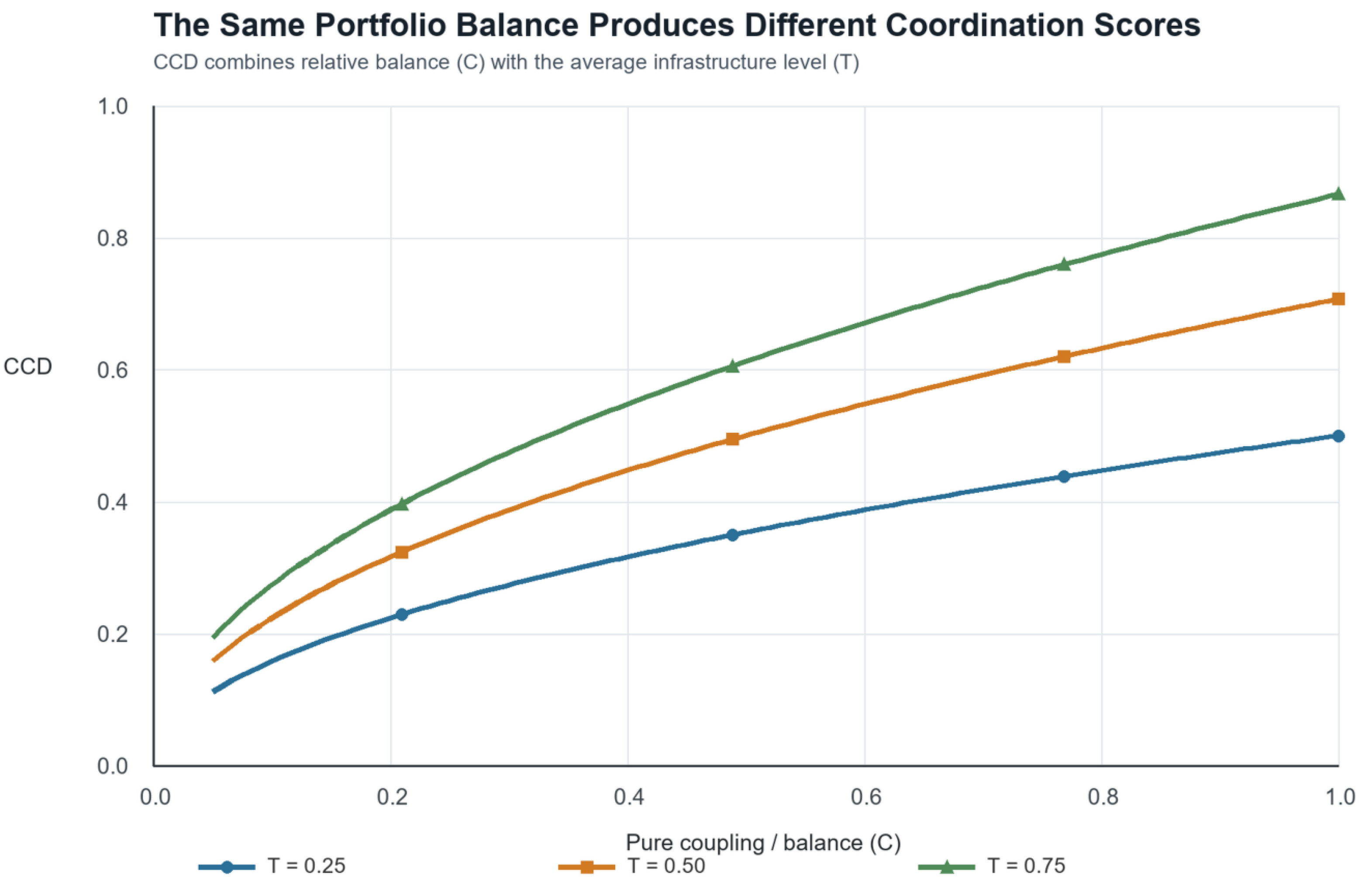
Figure 2.
Conditional associations of portfolio balance and portfolio level across the preferred and robustness specifications. Circles denote balance, squares denote level, and horizontal lines are 95% confidence intervals; the vertical line marks zero. Each pair enters jointly with the controls and fixed effects described in Section 3. The level association remains positive, whereas balance is smaller and sensitive to timing, outcome scope, and the transport proxy.
Figure 2.
Conditional associations of portfolio balance and portfolio level across the preferred and robustness specifications. Circles denote balance, squares denote level, and horizontal lines are 95% confidence intervals; the vertical line marks zero. Each pair enters jointly with the controls and fixed effects described in Section 3. The level association remains positive, whereas balance is smaller and sensitive to timing, outcome scope, and the transport proxy.
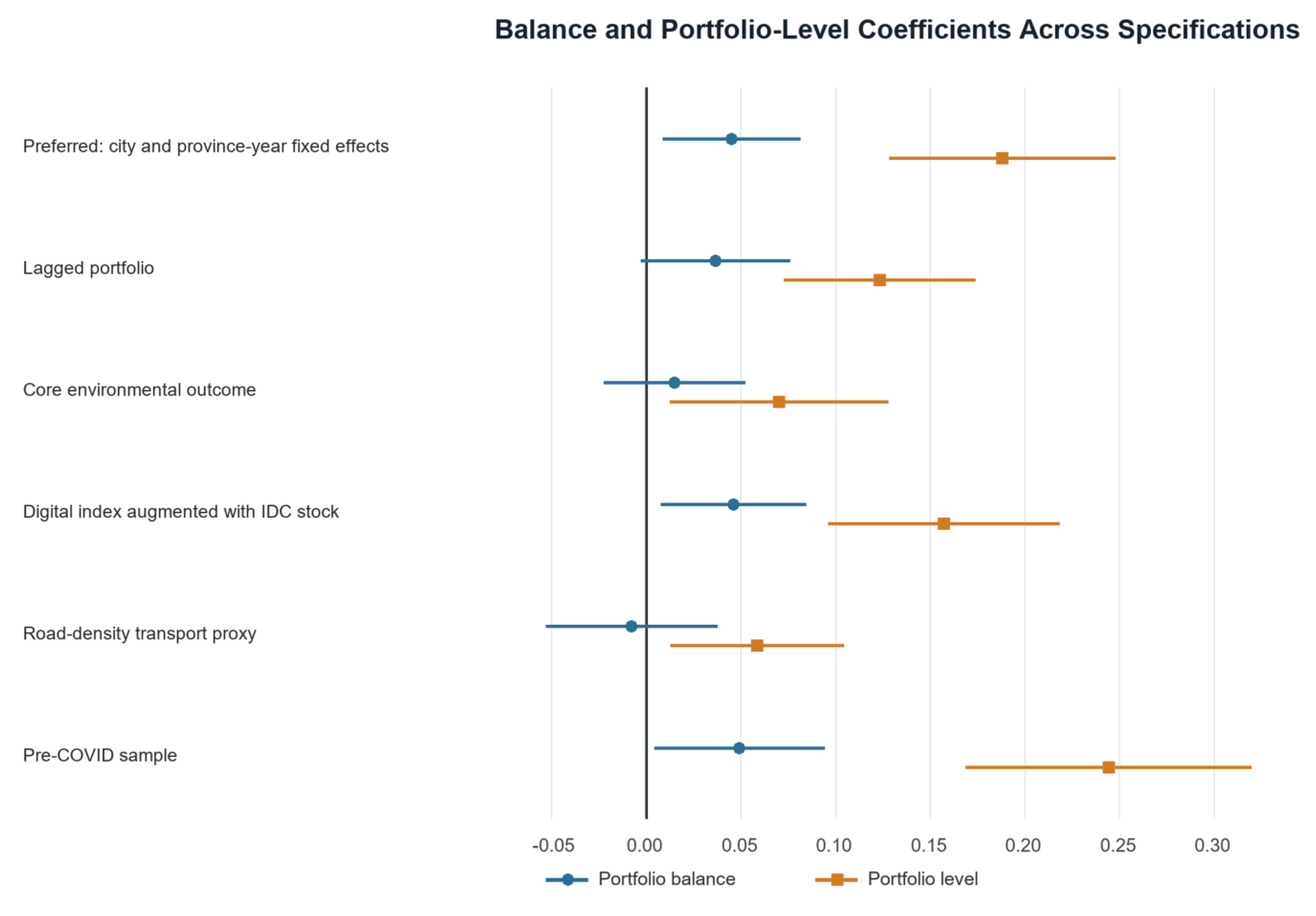
Figure 3.
Conditional associations by municipal environmental-service component. Circles denote portfolio balance, squares denote portfolio level, and horizontal lines are 95% confidence intervals; the vertical line marks zero. Balance is concentrated in water and gas access, while treatment and greening estimates remain statistically indistinguishable from zero, separating network-extension outcomes from facility- and governance-dependent outcomes.
Figure 3.
Conditional associations by municipal environmental-service component. Circles denote portfolio balance, squares denote portfolio level, and horizontal lines are 95% confidence intervals; the vertical line marks zero. Balance is concentrated in water and gas access, while treatment and greening estimates remain statistically indistinguishable from zero, separating network-extension outcomes from facility- and governance-dependent outcomes.
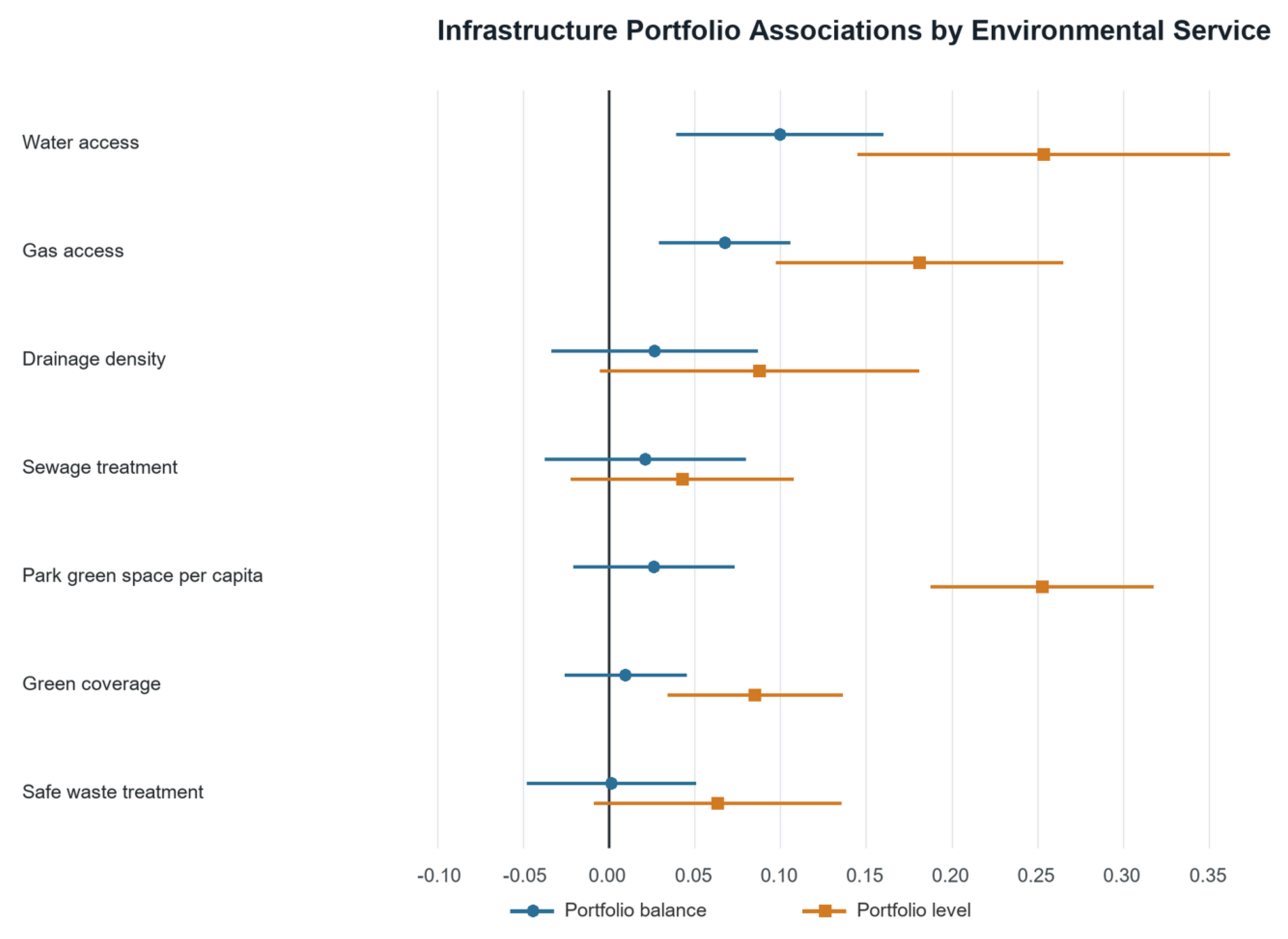

Table 1.
Descriptive statistics for the preferred complete-case sample.
| Variable | N | Mean | SD | P25 | Median | P75 |
| Environmental-service index | 6094 | 0.005 | 1.004 | -0.496 | 0.320 | 0.740 |
| Digital infrastructure rank | 6094 | -0.050 | 0.970 | -0.747 | -0.052 | 0.583 |
| Transport infrastructure rank | 6094 | -0.012 | 0.989 | -0.873 | -0.030 | 0.811 |
| Portfolio balance | 6094 | 0.006 | 0.987 | -0.221 | 0.434 | 0.644 |
| Portfolio level | 6094 | -0.035 | 0.971 | -0.727 | -0.068 | 0.617 |
| Conventional coupling-coordination degree | 6094 | -0.024 | 0.977 | -0.655 | 0.060 | 0.679 |
| Economic development | 6094 | 0.063 | 0.947 | -0.568 | 0.183 | 0.745 |
| Openness | 6094 | 0.024 | 1.015 | -0.520 | -0.346 | 0.080 |
| Service-sector share | 6094 | 0.021 | 0.991 | -0.687 | -0.057 | 0.644 |
| Human capital | 6094 | -0.014 | 0.942 | -0.600 | -0.343 | 0.143 |
| Government intervention | 6094 | -0.070 | 0.877 | -0.667 | -0.289 | 0.259 |
| Population density | 6094 | 0.072 | 0.906 | -0.429 | 0.165 | 0.697 |
Notes: Statistics use the 6094 complete observations in the preferred model. Continuous variables are winsorized and standardized as described in Section 3.
Table 2.
Conventional coordination metrics and their decomposition.
| Specification | Term | Coefficient | SE | p-value | N |
| Absolute rank gap | Gap | 0.016 | 0.028 | 0.575 | 6094 |
| Conventional CCD | CCD | 0.205*** | 0.025 | 0.000 | 6094 |
| Exact decomposition | Portfolio balance | 0.045** | 0.018 | 0.021 | 6094 |
| Exact decomposition | Portfolio level | 0.188*** | 0.030 | 0.000 | 6094 |
Notes: All regressions include six city controls, city fixed effects, and province-by-year fixed effects. The exact decomposition enters portfolio balance and portfolio level jointly. CCD = coupling-coordination degree. Standard errors are clustered by province. p-values use a Student-t reference with G - 1 degrees of freedom. * p < 0.10, ** p < 0.05, *** p < 0.01.
Table 3.
Portfolio balance and portfolio level: main estimates and robustness checks.
| Specification | Term | Coefficient | SE | p-value | N |
| City and year fixed effects | Portfolio balance | 0.051** | 0.024 | 0.040 | 6094 |
| City and year fixed effects | Portfolio level | 0.277*** | 0.043 | 0.000 | 6094 |
| Preferred: city and province-year fixed effects | Portfolio balance | 0.045** | 0.018 | 0.021 | 6094 |
| Preferred: city and province-year fixed effects | Portfolio level | 0.188*** | 0.030 | 0.000 | 6094 |
| Lagged portfolio | Portfolio balance | 0.037* | 0.020 | 0.078 | 5869 |
| Lagged portfolio | Portfolio level | 0.124*** | 0.026 | 0.000 | 5869 |
| Core environmental outcome | Portfolio balance | 0.015 | 0.019 | 0.434 | 5312 |
| Core environmental outcome | Portfolio level | 0.070** | 0.029 | 0.024 | 5312 |
| Digital index augmented with IDC stock | Portfolio balance | 0.046** | 0.020 | 0.025 | 6094 |
| Digital index augmented with IDC stock | Portfolio level | 0.157*** | 0.031 | 0.000 | 6094 |
| Road-density transport proxy | Portfolio balance | -0.007 | 0.023 | 0.747 | 5538 |
| Road-density transport proxy | Portfolio level | 0.059** | 0.023 | 0.018 | 5538 |
| Pre-COVID sample | Portfolio balance | 0.049** | 0.023 | 0.040 | 4724 |
| Pre-COVID sample | Portfolio level | 0.244*** | 0.038 | 0.000 | 4724 |
| Exclude municipalities | Portfolio balance | 0.045** | 0.019 | 0.023 | 6002 |
| Exclude municipalities | Portfolio level | 0.188*** | 0.031 | 0.000 | 6002 |
Notes: Each pair of rows comes from one regression in which balance and level enter jointly. The preferred and robustness models use the fixed effects stated in Section 3. IDC = internet data center. Standard errors are clustered by province. p-values use a Student-t reference with G - 1 degrees of freedom. * p < 0.10, ** p < 0.05, *** p < 0.01.
Table 4.
Portfolio balance and level across environmental-service components.
| Specification | Term | Coefficient | SE | p-value | N |
| Water access | Portfolio balance | 0.100*** | 0.031 | 0.003 | 6264 |
| Water access | Portfolio level | 0.254*** | 0.055 | 0.000 | 6264 |
| Gas access | Portfolio balance | 0.068*** | 0.019 | 0.002 | 6262 |
| Gas access | Portfolio level | 0.181*** | 0.043 | 0.000 | 6262 |
| Drainage density | Portfolio balance | 0.027 | 0.031 | 0.388 | 5178 |
| Drainage density | Portfolio level | 0.088* | 0.047 | 0.075 | 5178 |
| Sewage treatment | Portfolio balance | 0.021 | 0.030 | 0.481 | 5819 |
| Sewage treatment | Portfolio level | 0.043 | 0.033 | 0.205 | 5819 |
| Park green space per capita | Portfolio balance | 0.026 | 0.024 | 0.279 | 6270 |
| Park green space per capita | Portfolio level | 0.253*** | 0.033 | 0.000 | 6270 |
| Green coverage | Portfolio balance | 0.010 | 0.018 | 0.591 | 6265 |
| Green coverage | Portfolio level | 0.085*** | 0.026 | 0.003 | 6265 |
| Safe waste treatment | Portfolio balance | 0.002 | 0.025 | 0.946 | 5522 |
| Safe waste treatment | Portfolio level | 0.064* | 0.037 | 0.094 | 5522 |
Notes: Each outcome is standardized. Every regression includes balance, portfolio level, six controls, city fixed effects, and province-by-year fixed effects. Standard errors are clustered by province. p-values use a Student-t reference with G - 1 degrees of freedom. * p < 0.10, ** p < 0.05, *** p < 0.01.
Table 5.
Nonlinear digital-transport interaction estimates.
| Specification | Coefficient | SE | p-value | N |
| City and year fixed effects | -0.024 | 0.019 | 0.216 | 6094 |
| Preferred: city and province-year fixed effects | -0.029* | 0.017 | 0.099 | 6094 |
| Lagged portfolio | -0.034* | 0.018 | 0.072 | 5869 |
| Core environmental outcome | -0.002 | 0.023 | 0.940 | 5312 |
| Digital index augmented with IDC stock | -0.039*** | 0.014 | 0.010 | 6094 |
| Road-density transport proxy | -0.033 | 0.021 | 0.134 | 5538 |
| Pre-COVID sample | -0.038 | 0.022 | 0.102 | 4724 |
| Exclude municipalities | -0.029 | 0.017 | 0.102 | 6002 |
Notes: Each row reports the coefficient on the product of standardized digital and transport measures. Models include their main effects, six controls, and the fixed effects stated in Section 3. Standard errors are clustered by province. p-values use a Student-t reference with G - 1 degrees of freedom. * p < 0.10, ** p < 0.05, *** p < 0.01.
Table 6.
Fiscal-pressure and energy-intensity diagnostics.
| Specification | Term | Coefficient | SE | p-value | N |
| Fiscal pressure: Lower fiscal pressure | Portfolio balance | 0.047* | 0.023 | 0.051 | 2929 |
| Fiscal pressure: Lower fiscal pressure | Portfolio level | 0.171*** | 0.034 | 0.000 | 2929 |
| Fiscal pressure: Higher fiscal pressure | Portfolio balance | 0.068** | 0.027 | 0.018 | 3165 |
| Fiscal pressure: Higher fiscal pressure | Portfolio level | 0.202*** | 0.042 | 0.000 | 3165 |
| Energy intensity: Electricity intensity | Portfolio balance | 0.016 | 0.023 | 0.505 | 2909 |
| Energy intensity: Electricity intensity | Portfolio level | 0.044 | 0.035 | 0.221 | 2909 |
| Energy intensity: Industrial electricity intensity | Portfolio balance | 0.002 | 0.040 | 0.965 | 2908 |
| Energy intensity: Industrial electricity intensity | Portfolio level | 0.052 | 0.041 | 0.216 | 2908 |
Notes: Balance and level enter jointly. Fiscal-pressure rows are split-sample estimates; energy outcomes use the 2008-2019 electricity sample. All models include city and province-by-year fixed effects. Standard errors are clustered by province. p-values use a Student-t reference with G - 1 degrees of freedom. * p < 0.10, ** p < 0.05, *** p < 0.01.
Disclaimer/Publisher’s Note: The statements, opinions and data contained in all publications are solely those of the individual author(s) and contributor(s) and not of MDPI and/or the editor(s). MDPI and/or the editor(s) disclaim responsibility for any injury to people or property resulting from any ideas, methods, instructions or products referred to in the content. |
© 2026 by the authors. Licensee MDPI, Basel, Switzerland. This article is an open access article distributed under the terms and conditions of the Creative Commons Attribution (CC BY) license.
Copyright: This open access article is published under a Creative Commons CC BY 4.0 license, which permit the free download, distribution, and reuse, provided that the author and preprint are cited in any reuse.