

Submitted:
24 July 2026
Posted:
27 July 2026
You are already at the latest version
Abstract
Unsupervised clustering remains an essential technique for remote sensing image analysis because ground-truth labels are often unavailable or expensive to obtain. Conventional clustering algorithms, such as K-means and ISODATA, generally rely on distance-based similarity measures, require empirical parameter tuning or predefined numbers of clusters, and become less effective in high-dimensional spectral spaces. Moreover, spectral signatures acquired under different imaging conditions often vary in amplitude while preserving consistent local spectral structures. Unsupervised Wavelet-Feature Greedy Clustering Algorithm (WFGCA) is proposed for multispectral and hyperspectral remote sensing image classification, where multiscale wavelet transforms are employed to identify abrupt spectral structures, including local maxima, minima, and zero-crossing features, which provide robust descriptors of material characteristics. A wavelet-feature correlation coefficient is introduced to measure spectral similarity according to the positional consistency of these characteristic features rather than their amplitudes. Representative cluster centers are then selected using a greedy strategy that minimizes mutual correlation, automatically determining the number of clusters without prior knowledge of class distributions. The proposed method was evaluated using Landsat Thematic Mapper (TM) multispectral imagery and AVIRIS hyperspectral imagery. Parameter analyses demonstrate that the sampling interval, wavelet-feature threshold, orthogonality threshold, and wavelet decomposition scale effectively control clustering granularity and computational efficiency. Experimental results show that WFGCA produces homogeneous clustering results with well-preserved land-cover boundaries while substantially reducing computational cost through spatial sampling and compact wavelet-feature representations. The algorithm performs effectively on both multispectral and hyperspectral datasets without requiring iterative optimization or a predefined number of clusters. By exploiting stable multiscale spectral structures instead of absolute spectral amplitudes, WFGCA provides an efficient and robust unsupervised clustering framework for remote sensing image classification. The proposed wavelet-feature representation, correlation measure, and greedy cluster-center selection improve clustering adaptability, reduce redundancy among representative spectra, and offer flexible control over clustering resolution, making the method suitable for large-scale multispectral and hyperspectral remote sensing applications.
Keywords:
multispectral images
; hyperspectral images
; wavelet
; greedy algorithm
; clustering
1. Introduction
Hyperspectral remote sensing provides hundreds of contiguous spectral bands, enabling fine discrimination of land-cover materials and supporting applications such as environmental monitoring, precision agriculture, mineral exploration, ecological assessment, disaster monitoring, and military reconnaissance. Supervised deep-learning approaches have recently achieved remarkable performance. Firat et al. developed a hybrid 3D residual spatial–spectral convolutional network that leverages 3D CNN and ResNet architectures to extract deep spatio-spectral features [1,2]. Since ground-truth labels are often unavailable or expensive to acquire, unsupervised clustering remains an indispensable technique for organizing hyperspectral data into spectrally homogeneous regions before further analysis. Unsupervised clustering continues to attract considerable interest because it can exploit large volumes of unlabeled hyperspectral imagery and provide reliable initial information for image interpretation, target detection, and change analysis.
Early hyperspectral image clustering methods mainly relied on distance-based statistical algorithms such as K-means, ISODATA, and fuzzy C-means (FCM). K-means is computationally efficient but requires the number of clusters to be specified in advance [3,4,5] and is sensitive to initialization; its convergence speed is slow [6,7]. The clustering of each pixel reaches a balanced state through iteratively searching for the minimal spatial distance with all class centers. ISODATA introduces automatic cluster splitting and merging but depends heavily on multiple empirical thresholds [8,9,10]. Although ISODATA and ISMC [11,12] can determine the number of classes through self-iteration, the parameters are hard to determine, and some distance parameters should be adjusted according to changes in the number of dimensions. The Orthogonal Subspace Projection (OSP) method [13,14] selects primary targets or directions as a basis. It performs orthogonal projection on all pixels, subsequently identifying suboptimal targets or directions within the projected data. While the primary basis in the OSP method captures the vast majority of information—thereby reducing data dimensionality—the classification results are expressed as grayscale values of mixed pixels relative to the various basis vectors; consequently, the classification performance is not particularly distinct, and the number of spectral bands constrains the number of classes. Cui proposed a feature extraction method by computing vectorized pixel values from a very small local window to yield a superior BoW performance, but this reduces the classification accuracy [15,16]. Peng et al. introduced a graph-based deep spectral–spatial clustering network designed to capture structural relationships among pixels thoroughly. Their approach incorporates a self-expression-embedded multi-graph autoencoder that models high-order structural associations, enabling the extraction of robust spectral–spatial features together with a coherent global clustering structure [17]. FCM improves robustness by assigning fuzzy memberships but often suffers from high computational complexity and sensitivity to noise [18]. Fuzzy C-Means (FCM) improves clustering robustness by assigning soft memberships to pixels; nevertheless, it remains computationally expensive for high-dimensional hyperspectral data and is sensitive to noise and mixed pixels [19]. Graph-based approaches, including normalized cuts and spectral clustering, were subsequently introduced to preserve the intrinsic manifold structure of hyperspectral data and have demonstrated improved clustering performance on complex image scenes [20,21]. More recently, unsupervised representation learning, deep clustering networks, and self-supervised learning have significantly advanced hyperspectral image analysis by learning nonlinear feature representations directly from unlabeled data [22,23,24,25,26].
Although these approaches have achieved encouraging results, several challenges remain. Distance-based clustering methods generally measure similarity using Euclidean distance or related statistical metrics, which often become less discriminative in high-dimensional spectral spaces. Deep clustering approaches usually require computationally intensive network training, large numbers of hyperparameters, and considerable computational resources. Moreover, most existing methods compare complete spectral vectors or learned latent representations while largely overlooking an important characteristic of hyperspectral signatures: although spectral amplitudes may vary substantially because of illumination changes, atmospheric effects, sensor noise, or mixed pixels, spectra belonging to the same material usually exhibit local maxima, local minima, absorption valleys, and abrupt transitions at nearly identical spectral positions. These structural characteristics provide stable descriptors of material properties that are considerably less sensitive to spectral magnitude variations.
Wavelet transforms provide an effective multiscale framework for identifying abrupt spectral variations through zero-crossings and local extrema. Previous studies have applied wavelet analysis to hyperspectral feature extraction and segmentation. Acharyya combined wavelet theory with neuro-fuzzy techniques for segmentation purposes [27,28]. However, most existing wavelet-based methods utilize wavelet coefficients primarily as frequency-domain descriptors without explicitly exploiting the positional consistency of abrupt spectral features for unsupervised clustering. Furthermore, many existing methods still rely on iterative optimization procedures or computationally expensive similarity calculations.
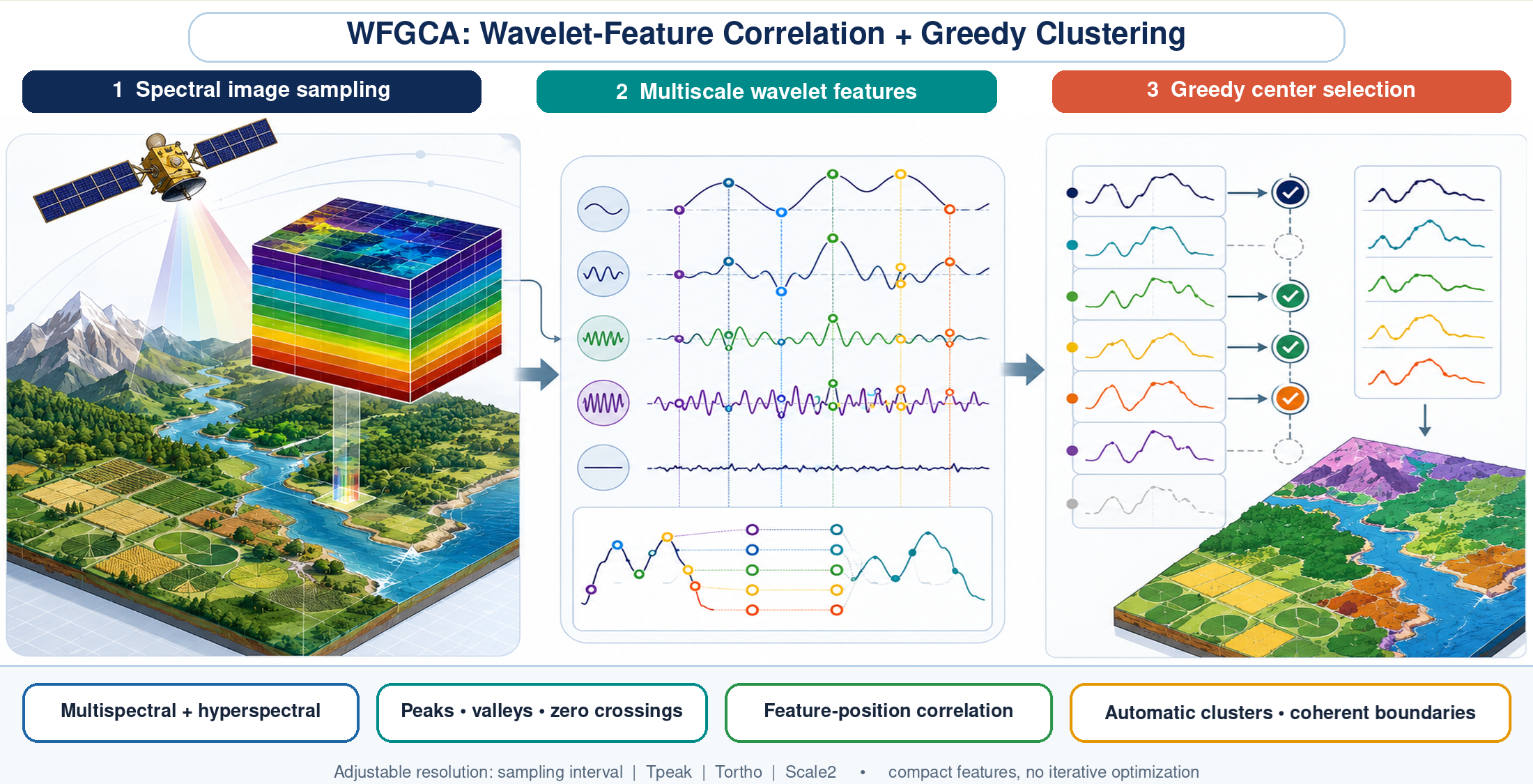
To address these limitations, this paper proposes an Unsupervised Wavelet-Feature Greedy Clustering Algorithm (WFGCA). Instead of measuring similarity directly from spectral amplitudes, the proposed method characterizes each spectrum by multiscale wavelet feature positions corresponding to abrupt spectral structures (Figure 1). A wavelet-feature correlation coefficient is developed to quantify similarity between spectral signatures according to the consistency of these characteristic positions. A greedy clustering strategy is then introduced to sequentially select representative cluster centers with minimal mutual correlation, thereby reducing redundancy while automatically determining the number of clusters without prior knowledge. This greedy clustering provides a global best solution. It resolves the limitations of the previously proposed wavelet-feature correlation ratio Markov clustering algorithm (WFCRMCA) [29], which only provides the best local solutions.
Compared with conventional clustering methods, the proposed WFGCA offers the following contributions: (1) a multiscale wavelet-feature representation that preserves stable spectral structures while reducing sensitivity to spectral magnitude variations; (2) a wavelet-feature correlation coefficient for efficient similarity measurement in high-dimensional hyperspectral data; (3) a greedy clustering algorithm that automatically determines representative cluster centers without requiring the number of clusters to be specified; (4) a computationally efficient unsupervised framework applicable to both multispectral Landsat TM and hyperspectral AVIRIS datasets. Experimental results demonstrate that WFGCA produces accurate clustering results while maintaining low computational complexity and providing flexible control over clustering granularity through several intuitive parameters.
2. Methods
2.1. Wavelet-Feature Correlation Coefficient
A material’s spectral signature is never identical across two acquisitions taken under different conditions. Yet, it tends to rise, fall, peak, or dip at nearly the same wavelength positions each time (Figure 1). This regularity is precisely what the bandpass wavelet kernel ψ(t) [30] is designed to pick up: defined as the first derivative of the Gaussian θ(t) in Equation (1), convolving a spectrum with ψ(t) turns each of the four abrupt-signal shapes in Figure 2a–d, including downward, upward, protruding, and concave, into either a zero-crossing or a local extremum at the filter’s output (Figure 2a′–d′).
For some remote sensing data characterized by significant interference or a high proportion of mixed pixels, the locations of abrupt change points may shift, or numerous minor fluctuations may be present. These issues can be addressed by clustering based on selected high-level detail components, applying fuzzy processing to account for positional shifts, or setting a modulus maxima threshold to eliminate insignificant fluctuation signals. Ranked by importance, the four signal types run, from most to least significant: downward, upward, protruding, and concave (Figure 2). In scenes with a large fraction of mixed pixels, the exact location of these features can drift or break into minor spurious fluctuations; setting an upper threshold filters this out, leaving only the strongest minutiae — those that persist at the coarser wavelet scales — for the analysis.
Locating these abrupt signals and recording where they fall is, in essence, what wavelet-feature clustering does. The wavelet coefficients themselves come from Mallat’s fast decomposition algorithm [31,32], Equation (2); from these, upward-step maximum points and downward-step minimum points whose magnitude exceeds a threshold are located and marked.
where is the total band count, and are the low-pass and high-pass filter coefficients, and and are the -th low-pass and high-pass filtered values at decomposition level .
Pixel-to-pixel similarity is then quantified by the correlation coefficient (CC), , in Equation (3), computed over the -level subset of minutiae taken from the full -level decomposition. Rather than Euclidean distance, a geometric measure of how far apart two spectral vectors sit, judges closeness purely from how many partial-minutiae positions the two vectors share, and it is this measure that drives the clustering step.
where is the -th feature value of sampled pixel , and counts how many feature positions satisfy the stated condition. A binary flag can mark whether a given position is informative enough to be worth including in the comparison. In the special case where , the number of bits entering the comparison works out to .
Working with only a partial set of high-scale minutiae pays off most in scenes with heavy pixel mixing: it keeps the sheer number of minutiae from overwhelming the comparison, at the cost of a mild blurring effect that in practice still produces workable clusters. This same lever, adjusting scale, is what lets the method move between fine-grained and coarse-grained classification. And because comparing abrupt-point locations is computationally cheap, adding more minutiae to the reference set adds little to overall clustering time. As a practical default, expanded multispectral bands are typically processed with , while hyperspectral bands more often use .
2.2. Expanding Bands Method for Multispectral Images
The number of bands available in multispectral imagery (TM images, for example, provide only seven bands) is often insufficient for the wavelet transform to extract enough informative feature points. To address this, we first exclude bands that are heavily affected by noise, then expand the remaining bands using second-order and nonlinear correlation functions so that more wavelet features can be detected. This band-expansion method [3] is defined as follows.
- Second-order correlated bands: the auto-correlated band set and the cross-correlated band set , .
- Nonlinearly correlated bands: the square-root band set and the logarithmic band set .
- Combining the bands generated in (1) and (2) with the original first-order bands, , yields a new dataset containing bands.
Although this expansion appears to add data-processing complexity, its effect on clustering speed is more favorable than it first seems. When only a few classes are present, each class tends to contain a large number of pixels, and updating the center of a large class is relatively slow. Because the expanded band set resolves more distinguishable classes, individual classes remain smaller on average, which keeps center computation efficient. As a result, the proposed band-expansion method improves both clustering accuracy and clustering speed for multispectral data.
2.3. Greedy Clustering Algorithm
The similarity between two remotely sensed pixels is quantified using the correlation coefficient (CC), which is computed from the number of common abrupt spectral features shared by their spectral signatures. A smaller CC indicates weaker similarity and therefore a larger separation between the two pixels in the feature space. Consequently, the objective of clustering is to identify a set of representative pixels that exhibit the lowest mutual correlations, thereby maximizing the diversity among cluster centers.
The proposed greedy clustering algorithm (GCA) selects representative pixels sequentially according to two criteria. First, a small number of representative samples should capture the dominant information contained in the entire dataset. Second, the correlation coefficient between any pair of selected cluster centers must remain below a predefined threshold, . This threshold controls the maximum allowable similarity among cluster centers and guarantees that each newly selected center contributes additional information rather than duplicating existing representatives.
Inspired by the concept of orthogonal projection, each selected cluster center is regarded as an independent basis vector describing the feature space. The purpose of selecting a new center is to maximize its independence from the previously chosen centers. Therefore, the cumulative correlation among all selected centers should be minimized. Samples chosen earlier represent the most significant characteristics of the dataset, whereas later selections progressively describe finer details. Because each selection is made based on the current best choice without reconsidering previous decisions, the procedure follows a greedy optimization strategy, referred to as the Greedy Clustering Algorithm (GCA).
The selection process begins with an initial representative sample, denoted as . Each subsequent candidate is evaluated according to its correlations with the already selected centers. The optimization objective is expressed by the minimum-energy criterion [33]:
where denotes the correlation coefficient between samples and ; a larger value of indicates stronger similarity between the two samples. The threshold plays a role analogous to the error tolerance used in pseudo-inverse computation and determines the admissible correlation among clustering centers.
Following the priority and minimum-energy principles, the GCA evaluates every candidate sample as a potential cluster center. Let denote the set of selected centers, the remaining candidate set, and the total number of samples. For each candidate pixel, an importance measure is defined as the sum of its correlation coefficients with all previously selected centers,
A smaller value of indicates that the candidate contributes more new information and therefore has a higher priority for selection.
The complete GCA procedure is summarized below.
Initialize the selected set and the candidate set .
Select an initial sample as the first cluster center, move it from to , and compute the correlation sums for all remaining candidates using (5).
Sort the candidates in ascending order of . Beginning with the smallest value, examine each candidate sequentially. A candidate is accepted as a new cluster center only if its correlation coefficient with every previously selected center satisfies
Once accepted, the sample is transferred from to , and the correlation sums are updated.
Repeat Step 3 until no additional samples satisfy the correlation constraint. The final set constitutes the cluster centers.
Assign every pixel to the cluster whose center has the largest correlation coefficient with that pixel.
Unlike conventional iterative clustering approaches, such as K-means, which repeatedly relocate cluster centers until convergence, the proposed GCA directly identifies representative centers through a greedy search. Iterative methods often allocate excessive cluster centers to densely populated regions, increasing redundancy while overlooking subtle but informative structures. Moreover, the required number of clusters must usually be specified in advance.
The proposed GCA avoids these limitations by selecting cluster centers in descending order of information content while enforcing low pairwise correlations. Consequently, the number of clusters is determined automatically according to both the correlation threshold and the complexity of the image scene. A larger value of imposes a stricter independence requirement, allowing more detailed image structures to be represented and generally producing a larger number of cluster centers. Conversely, scenes with relatively homogeneous land-cover types exhibit higher spectral similarity among pixels, resulting in fewer selected centers.
2.4. Wavelet-Feature Greedy Clustering Algorithm (WFGCA)
The proposed Greedy Clustering Algorithm (GCA) can be extended from the original spectral space to the wavelet feature space by utilizing abrupt spectral features extracted through multiscale wavelet analysis. This extension is referred to as the Wavelet-Feature Greedy Clustering Algorithm (WFGCA). Instead of directly comparing spectral vectors, WFGCA measures pixel similarity based on the distribution of their wavelet-derived feature points, enabling more reliable discrimination of hyperspectral signatures. The implementation of WFGCA is summarized as follows.
- Input parameters: and are the sampling steps along the horizontal and vertical directions in the remotely sensed images. b is the spectral band number, m is the column number, and n is the row number. is the maximal scale of the applied wavelet transform, normally no more than . The wavelet minutiae from to will be clustered according to (3).
- Sample all the pixels evenly at spatial steps with as the x-coordinate step and as the y-coordinate step, creating Ns sampled pixels.
- Apply GCA to the minutiae sections for the wavelet coefficients and achieve clustering centers with CC between each other less than .
- Select sample t0 as the first object, according to (7), initialize the selected sample set I, and the waiting sample set J.
- In J, choose the sample , with which the CC of each sample in I is less than, and the sum of these CCs is minimal according to (8). If none is found, then clustering ends and goes to step 7; otherwise, add i to object set I and iterate this process.
- Each pixel , according to the clustering centers created in step 4, is clustered into the class whose center has the maximal CC with .
The proposed WFGCA possesses several computational and practical advantages.
- Linear computational complexity. Assuming that cluster centers are generated from sampled pixels, only correlation evaluations are required. Consequently, the overall computational complexity is approximately , making the algorithm suitable for large hyperspectral datasets.
- Efficient similarity computation. Unlike Euclidean-distance-based methods that require extensive floating-point operations, the proposed correlation coefficient is obtained simply by counting matched abrupt spectral features occurring at identical spectral locations. This significantly reduces computational overhead and accelerates the clustering process.
- Low memory consumption. During the greedy search, only the correlation values between candidate pixels and the currently selected cluster centers are maintained. Therefore, the algorithm avoids storing a complete pairwise similarity matrix, resulting in substantially lower memory requirements.
- Adaptive clustering resolution. The clustering granularity can be adjusted by modifying three parameters: , , and . Increasing permits finer distinctions among similar spectral patterns, thereby producing a larger number of cluster centers. Conversely, lower threshold values generate fewer clusters by emphasizing only the dominant spectral structures.
3. Results
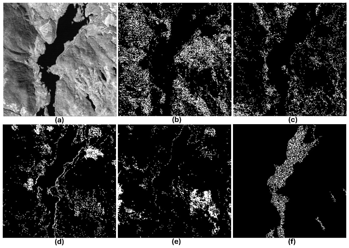
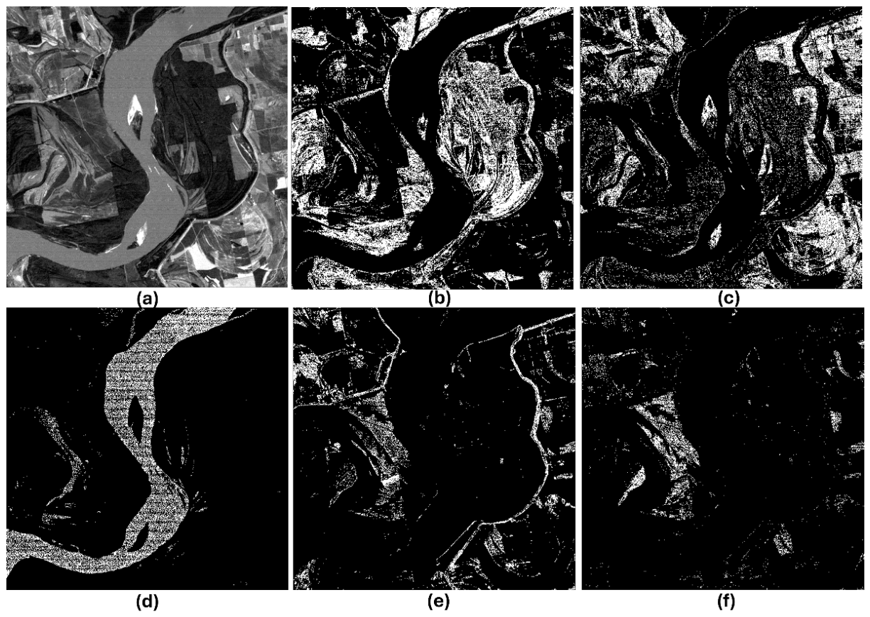
The characteristics of wavelet-feature clustering were tested using WFMCA analysis of TM and AVIRIS data (Figure 3a and Figure 9a), with classified pixels shown in white.
3.1. AVIRIS Data
Evaluation data were collected by the AVIRIS airborne imaging spectrometer on 2 September 1993, over the SEIDAM Sooke Lake study area on Vancouver Island, British Columbia, Canada [36,37] (Figure 3a). The sensor recorded 224 contiguous spectral bands covering the 410–2450 nm range. Although the sensor’s native ground sampling distance was approximately 20 m, the version of the dataset used here was supplied as a georeferenced product resampled to 25 m. The extracted area has a width of 256 pixels and height of 256 pixels. The WFGCA uses all 224 bands for classification algorithm analysis.
After 5*5 down-sampling, the top three-scale wavelet features from the total five-scale wavelet decomposition (=3/5) were selected for clustering. When =0.8, 125 classes were created, and the major five clustering results were shown in Figure 3b-5f. The division results are quite ideal. From Table 1, when the 1st and 2nd scale minutiae are used for clustering, the number of classes increases sharply, but clustering accuracy improves only slightly because controls it. If only the minutiae from the 3rd to 5th scales are used for clustering, and is increased to 0.95, the number of classes doubles, while clustering accuracy and speed are clearly improved. Therefore, for hyperspectral clustering, partial high-scale minutiae sections and higher Tortho values can ensure not only a reasonable number of classes but also fairly high clustering accuracy. All the pixels can be identified, according to their spectra, to be forest (Figure 3b), levees (Figure 3c), wetlands (Figure 3d), mountain peaks (Figure 3e), or water (Figure 3f).
3.1.1. Sampling Interval Effect
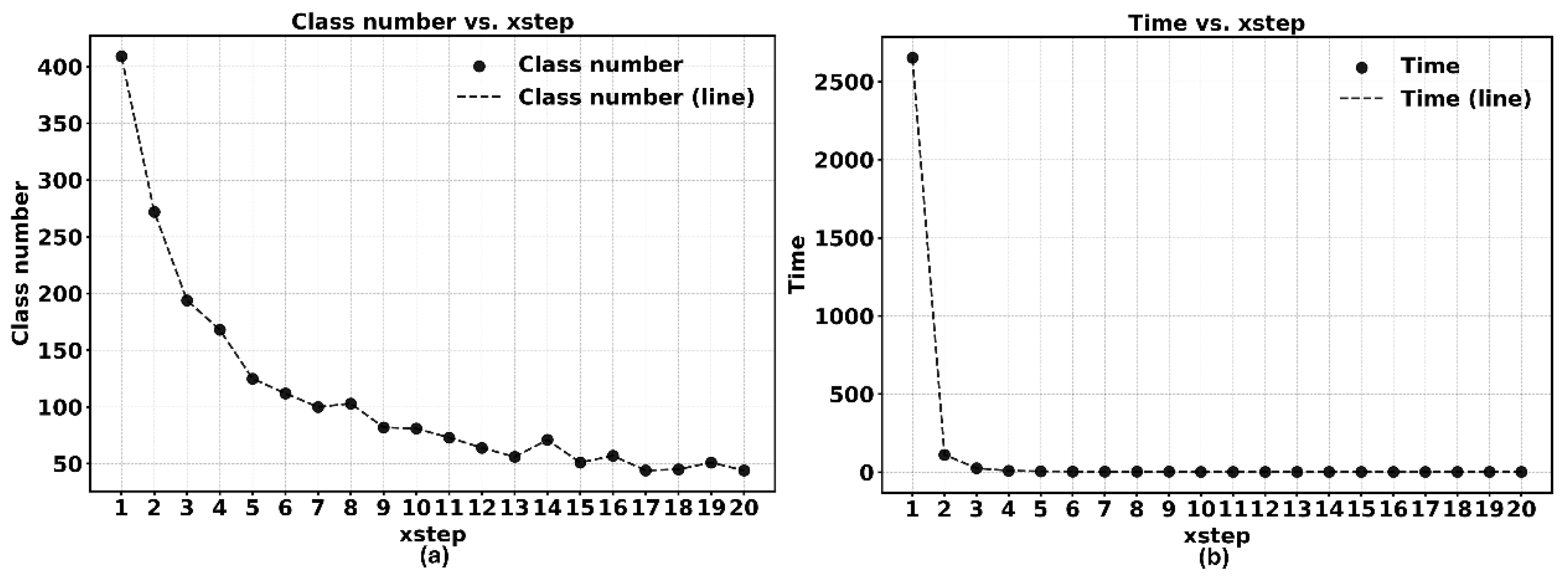
Increasing the spatial sampling interval xstep sharply reduces both the number of clusters and the WFGCA runtime. Figure 4 and Table 2 show that from xstep = 1 to 5, the number of classes falls from 409 to 125, while runtime decreases from 2652 to 6 s. At xstep = 10, only 81 classes are generated in 3 s, and at 20 the result is 44 classes in 2 s. Thus, full-resolution sampling provides the finest partition but incurs a very high computational cost.
Figure 3.
(a) The 50th band Sook Lake AVIRIS image after gray balance. (b)-(f) are the first five major signals after WFGCA clustering with xstep=ystep=5, Tpeak=5, Tortho=0.8, = 3/5.
Figure 3.
(a) The 50th band Sook Lake AVIRIS image after gray balance. (b)-(f) are the first five major signals after WFGCA clustering with xstep=ystep=5, Tpeak=5, Tortho=0.8, = 3/5.
The decline is strongly nonlinear. Increasing xstep from 1 to 2 alone reduces runtime by 95.8% (2652 to 112 s), whereas the class number decreases by 33.5% (409 to 272). Beyond approximately xstep = 9, runtime remains between 2 and 4 s, and the class number fluctuates within a narrower range of 44–81, indicating diminishing computational returns from further subsampling. These small class-count fluctuations reflect changes in which the sampling grid retains representative pixels.
These results reveal a tradeoff between clustering granularity and efficiency: smaller intervals retain more candidate spectra and produce more classes, whereas larger intervals provide faster but coarser partitions. For this AVIRIS dataset, xstep = 5 offers a practical compromise, producing 125 classes in 6 s and reducing runtime by approximately 99.8% relative to xstep = 1.
Figure 4.
Effect of on (a) class number and (b) time is investigated using WFGCA clustering with xstep=ystep, Tpeak=5, Tortho=0.8, and = 5/7.
Figure 4.
Effect of on (a) class number and (b) time is investigated using WFGCA clustering with xstep=ystep, Tpeak=5, Tortho=0.8, and = 5/7.
3.1.2. Band Number
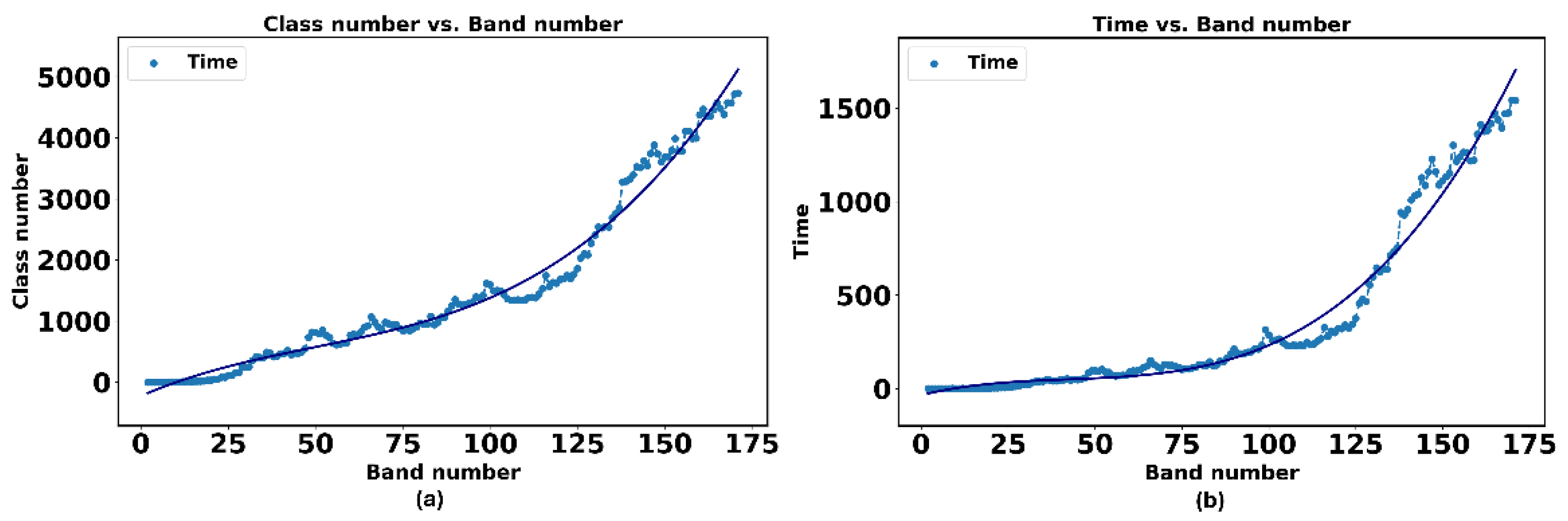
Band number b controls the spectral dimensionality available to WFGCA. Figure 5 shows that both class number and runtime increase nonlinearly as the band number grows. Across the tested range, the class number rises from approximately 1 at b = 2 to nearly 5000 at b = 175, while runtime increases from approximately 1 s to about 1500 s. Growth is relatively gradual at lower band counts but accelerates markedly beyond roughly 125–135 bands, with local fluctuations reflecting differences in the information contributed by individual bands. Additional bands therefore enable finer spectral separation but also expand the feature space and computational burden; band selection or dimensionality reduction may be beneficial when the full spectral resolution is unnecessary.
Figure 5.
The effect of band number over (a) class number and (b) time is investigated using WFGCA clustering with xstep=ystep=5, Tpeak=5, Tortho=0.8, and = 5/7.
Figure 5.
The effect of band number over (a) class number and (b) time is investigated using WFGCA clustering with xstep=ystep=5, Tpeak=5, Tortho=0.8, and = 5/7.
3.1.3. Tpeak Effect
Increasing Tpeak produces a nonlinear reduction in both class number and runtime. In Figure 6 and Table 2, from Tpeak = 1 to 5, the class number decreases from 345 to 125, and runtime falls from 14 to 6 s. The decline then slows: at Tpeak = 8, WFGCA generates 93 classes in 4 s, and over Tpeak = 8–16 the result remains within 83–93 classes and 4–5 s. This plateau indicates that thresholds above approximately 8 provide little additional computational benefit. A low Tpeak retains weaker peaks and yields a finer partition, whereas a high value suppresses them and produces fewer classes. For this dataset, Tpeak = 5 provides a practical balance, retaining 125 classes with a runtime of 6 s.
3.1.4. Tortho Effect
Tortho has a nonlinear effect on clustering granularity. In Figure 7 and Table 3, the class number rises only from 3 to 13 as Tortho increases from 0.1 to 0.5, then sharply to 28, 59, 125, and 270 at 0.6–0.9, before leveling off at 280 for 0.95. Runtime remains 1–2 s through 0.6 and then rises to 4, 6, 11, and 10 s at 0.7–0.95. Despite small timing fluctuations, computational costs generally increase with class count. Thus, higher Tortho values produce finer clustering at greater cost, while 0.7–0.8 offers a practical balance for this dataset.
3.1.5. Scale2 Effect
Scale2 has a strongly nonlinear effect on clustering granularity and computational cost. From Figure 8 and Table 4, for Scale2 = 1–3, WFGCA produces only 1, 1, and 2 classes, respectively, with a runtime of 2 s. The class number then increases to 25 at Scale2 = 4, 125 at 5, 414 at 6, and 2453 at 7, while runtime rises from 1 s at 4 to 6, 26, and 305 s at 5–7. Relative to Scale2 = 5, including the second- and first-scale minutiae at values of 6 and 7 increases the class number by approximately 3.3 and 19.6 times, respectively, but increases runtime by approximately 4.3 and 50.8 times. Thus, intermediate values of 4–5 provide a more controlled balance, whereas 6–7 should be used only when very fine class separation justifies the substantially greater computational cost.
3.2. TM Data
To evaluate the effectiveness of the proposed Wavelet-Feature Greedy Clustering Algorithm (WFGCA) on multispectral remote sensing imagery, experiments were conducted using the Landsat Thematic Mapper (TM) dataset for the Mississippi River (scene Y4 018 116 055X0 [38], 512*512, 8 bit/pixel) shown in Figure 9a. The test scene contains several representative land-cover types, including water bodies, agricultural fields, vegetation, bare soil, and urban areas. Compared with hyperspectral imagery, Landsat TM provides only a limited number of spectral bands; therefore, discrimination of spectrally similar materials depends primarily on the clustering algorithm’s ability to exploit the characteristic spectral structures contained in the available bands. In WFGCA, the seven bands were expanded to 49 bands, including original data (1-7), second-order auto-correlated bands (8-14), second-order cross-correlated bands (15-35), square root function bands (36-42), and logarithmic function bands (43-49).
The quantitative evaluation summarized in Table 5 further confirms the superiority of the proposed algorithm. After 5*5 down-sampling, the increase in class number from second-order auto-correlation (8-14) is limited to 2, but the expanded bands from second-order cross-correlation (15-35) provide 57 classes and the square root function 90 classes, enhancing classification accuracy. The logarithmic function does not contribute to more detailed classes, even lower down the class number from 90 to 87. Figure 9b-f are the five major classes chosen from the total 87 classes, where the band number is 49, Tortho is 5, Tortho is 0.8, uses 5, and is the same as . All the pixels can be identified by their spectra as beach (Figure 9b), plow land or meadow (Figure 9c), river channel (Figure 9d), dyke (Figure 9e), and the slope on the bank (Figure 9f).

Table 5.
Effect of with xstep=ystep=5, Tpeak=5, Tortho=0.8, and =7.
| Class number | Time | ||
|---|---|---|---|
| 1 | 1 | 2 | |
| 2 | 1 | 2 | |
| 3 | 2 | 2 | |
| 4 | 25 | 1 | |
| 5 | 125 | 6 | |
| 6 | 414 | 26 | |
| 7 | 2453 | 305 |
Table 6.
Mississippi TM image: influence of expanded band number on WFGCA (5*5 sampling).
| Band no. | Tpeak | Tortho | Scale | Scale2 | Class number | time |
|---|---|---|---|---|---|---|
| 7 | 5 | 0.8 | 2 | 2 | 1 | 1 |
| 14 | 5 | 0.8 | 3 | 3 | 3 | 14 |
| 35 | 5 | 0.8 | 5 | 5 | 57 | 13 |
| 42 | 5 | 0.8 | 5 | 5 | 90 | 20 |
| 49 | 5 | 0.8 | 5 | 5 | 87 | 20 |
Figure 9.
Mississippi TM remotely sensed image: Figure 1. (a) The 3rd band Mississippi TM image after gray balance. b-f are WFGCA clustering the first five main signals with Tortho=0.8.
Figure 9.
Mississippi TM remotely sensed image: Figure 1. (a) The 3rd band Mississippi TM image after gray balance. b-f are WFGCA clustering the first five main signals with Tortho=0.8.
5. Discussion
The experimental results support the central premise of WFGCA: the positional consistency of multiscale spectral features can provide a compact basis for unsupervised classification when absolute spectral amplitudes vary. In the AVIRIS experiment, the method separated spectra associated with forest, levees, wetlands, mountain peaks, and water. In contrast, the Landsat TM experiment produced spatially coherent groups associated with beach, plowed land or meadow, river channel, dike, and bank slope. These outcomes are consistent with the motivation presented in the Introduction and with the method described in Section 2, because cluster assignment depends on shared extrema and abrupt-transition positions rather than on the Euclidean separation of complete spectral vectors. The findings therefore indicate that wavelet-feature locations retain material-discriminative information in both hyperspectral and multispectral settings.
The AVIRIS parameter analyses clarify how each component of WFGCA controls the balance between clustering granularity and computational cost—increasing the spatial sampling interval from 1 to 5 reduced runtime from 2652 to 6 s (approximately 99.8%) while decreasing the number of clusters from 409 to 125, demonstrating that representative spatial sampling is the main source of computational savings. Increasing Tpeak removed weak wavelet extrema and reduced both class count and runtime, with limited additional benefit above approximately 8. Tortho controlled the admissible similarity among selected centers: values of 0.7-0.8 provided a practical intermediate resolution, whereas larger values produced many more centers at greater cost. Scale2 had the strongest nonlinear effect; incorporating finer-scale minutiae increased the number of classes from 125 at Scale2 = 5 to 414 and 2453 at Scale2 = 6 and 7, respectively, while runtime increased from 6 to 26 and 305 s. Collectively, these results confirm that sampling interval, feature threshold, orthogonality threshold, and decomposition scale serve distinct but complementary roles in controlling efficiency and resolution.
The multispectral experiment further demonstrates why band expansion is needed when only a small number of original bands are available. Expanding the seven Landsat TM bands to 49 bands created additional wavelet-feature positions that the correlation measure could use. However, the contributions of the transformations were unequal: second-order autocorrelation added only two clusters, whereas cross-correlation increased the class count to 57 and the square-root transformation increased it to 90. Adding logarithmic bands did not improve granularity and reduced the final count from 90 to 87. This result suggests that band expansion should be selective rather than automatic; transformations that introduce complementary spectral structure are useful, whereas redundant transformations may add computation without improving discrimination.
Relative to K-means, ISODATA/ISMC, and projection-based approaches discussed in the Introduction, WFGCA offers two practical advantages. First, it does not require a predefined number of clusters; the number emerges from scene complexity and the center-correlation threshold. Second, it avoids repeated center relocation and uses compact feature matching rather than full-vector Euclidean-distance calculations. The resulting clusters are therefore interpretable as groups organized around representative spectra with limited mutual correlation. Nevertheless, the present experiments do not establish statistical superiority over these methods, because no common ground-truth labels or quantitative external validity measures were used. The observed homogeneous regions, preserved boundaries, class counts, and runtimes demonstrate feasibility and parameter behavior, but claims about classification accuracy should be confirmed through controlled benchmark comparisons.
Several limitations should guide interpretation of the results. WFGCA is unsupervised, so its clusters are spectral groupings rather than guaranteed semantic land-cover classes, and the class count can substantially exceed the number of broad cover categories in a scene. The selected parameters remain dataset dependent, particularly at fine wavelet scales where noise and mixed pixels can generate many additional features. Uniform spatial sampling may also omit rare materials that do not fall on the sampling grid, and the current spectral-only formulation does not explicitly use neighborhood context, which could improve robustness in heterogeneous regions.
Future work should therefore evaluate WFGCA on labeled hyperspectral benchmarks using clustering accuracy, normalized mutual information, adjusted Rand index, boundary preservation, runtime, and memory consumption under a common experimental protocol. Adaptive selection of Tpeak, Tortho, sampling interval, and Scale2 could reduce manual tuning, while rare-target-aware or multistage sampling could limit the loss of small classes. Incorporating spatial-context constraints, automated selection of informative expanded bands, and parallel implementation would further improve robustness and scalability. Extensions to multisensor fusion and temporal remote sensing should be investigated only after these benchmark evaluations establish when positional wavelet features provide advantages over amplitude-based and learned representations.
6. Conclusions
The proposed Wavelet-Feature Greedy Clustering Algorithm (WFGCA) for unsupervised multispectral and hyperspectral remote sensing image classification addresses several limitations of conventional clustering algorithms, including their dependence on distance-based similarity measures, empirical parameter selection, predefined numbers of clusters, and sensitivity to spectral amplitude variations. Instead of comparing complete spectral vectors, WFGCA characterizes spectral signatures using multiscale wavelet-derived feature points and evaluates spectral similarity through a wavelet-feature correlation coefficient that emphasizes the positional consistency of characteristic spectral structures. Representative cluster centers are then selected using a greedy strategy that automatically determines the clustering structure while reducing redundancy among representative spectra.
Experimental evaluations using Landsat TM multispectral imagery and AVIRIS hyperspectral imagery demonstrate the effectiveness of the proposed approach. The parameter analyses show that the spatial sampling interval, wavelet-feature threshold, orthogonality threshold, and wavelet decomposition scale provide effective control over clustering resolution and computational efficiency. Appropriate parameter selection substantially reduces computational cost while preserving the principal spectral characteristics required for accurate clustering. These results indicate that representing spectra by stable wavelet features improves robustness to spectral variability while maintaining the ability to discriminate different surface materials.
An important advantage of WFGCA is its computational efficiency. The combination of spatial sampling, compact wavelet-feature representations, and greedy representative-spectrum selection significantly reduces the number of similarity calculations required during clustering. Unlike iterative optimization algorithms that require repeated updates of cluster centers or empirical splitting and merging operations, the proposed framework automatically identifies representative cluster centers without requiring a predefined number of classes, making it well suited for large-scale remote sensing image analysis.
Although the proposed method demonstrates strong performance on both multispectral and hyperspectral datasets, several opportunities remain for further improvement. Future work will investigate adaptive parameter optimization to reduce manual parameter tuning, incorporate spatial-context information to improve the discrimination of complex heterogeneous regions, and develop parallel implementations suitable for high-performance computing platforms. In addition, extending the wavelet-feature correlation framework to emerging remote sensing modalities, such as multisensor data fusion and time-series image analysis, may further improve the applicability of the proposed algorithm to large-scale Earth observation tasks.
Overall, the proposed WFGCA provides an efficient, robust, and adaptive framework for unsupervised remote sensing image classification. By combining multiscale wavelet-feature extraction, wavelet-feature correlation analysis, and greedy representative-spectrum selection, the method effectively balances clustering accuracy, computational efficiency, and automation, offering a practical solution for the unsupervised analysis of multispectral and hyperspectral remote sensing imagery.
Funding
This research received funding support from the 2025 Yale University ASCEND Initiative and the 2025 NASA MPLAN.
Institutional Review Board Statement
Not applicable.
Informed Consent Statement
Not applicable.
Data Availability Statement
All data are publicly available and referenced in the paper.
Conflicts of Interest
The authors declare no conflicts of interest.
References
- Ju, W., Fang, Z., Gu, Y., Liu, Z., Long, Q., Qiao, Z., ... & Zhang, M. (2024). A comprehensive survey on deep graph representation learning. Neural Networks, 173, 106207.
- Firat, H.; Asker, M.E.; Bayindir, M.I.; Hanbay, D. 3D residual spatial–spectral convolution network for hyperspectral remote sensing image classification. Neural Comput. Appl. 2023, 35, 4479–4497.
- MacQueen, J. Some Methods for Classification and Analysis of Multivariate Observations. Proc. Fifth Berkeley Symposium, 1967.
- Wang, Z. Residual Clustering Based Lossless Compression for Remotely Sensed Images. In Proceedings of the 2018 IEEE International Symposium on Signal Processing and Information Technology (ISSPIT), Louisville, KY, USA, 6–8 December 2018; pp. 536–539. [CrossRef]
- Wang, Z. Entropy Analysis for Clustering-Based Lossless Compression of Remotely Sensed Images. In Proceedings of the 2021 IEEE International Conference on Big Data (Big Data), Orlando, FL, USA, 15–18 December 2021; pp. 4220–4223. [CrossRef]
- Theodoridis, S.; Koutroumba, K. Pattern Recognition, 4th ed.; Academic Press: Cambridge, MA, USA, 2008; pp. 741–745.
- Ikotun, A.M.; Ezugwu, A.E.; Abualigah, L.; Abuhaija, B.; Heming, J. K-means Clustering Algorithms: A Comprehensive Review, Variants Analysis, and Advances in the Era of Big Data. Inf. Sci. 2023, 622, 178–210.
- Ball, G.H.; Hall, D.J. ISODATA, A Novel Method of Data Analysis and Pattern Classification. Stanford Research Institute, 1965.
- Soto de la Cruz, R.; Castro-Espinoza, F.A.; Soto, L. Isodata-Based Method for Clustering Survey Responses with Mixed Data: The 2021 StackOverflow Developer Survey. Comput. Sist. 2023, 27, 173–182.
- Arai, K. Improved ISODATA Clustering Method with Parameter Estimation based on Genetic Algorithm. Int. J. Adv. Comput. Sci. Appl. 2022, 13, 187–193.
- Simpson, J.J.; McIntyre, T.J.; Sienko, M. An Improved Hybrid Clustering Algorithm for Natural Scenes. IEEE Trans. Geosci. Remote Sens. 2000, 38, 1016–1032.
- Bo, L.; Bretschneider, T. D-ISMC: A distributed unsupervised classification algorithm for optical satellite imagery. In Proceedings of the 2003 IEEE International Geoscience and Remote Sensing Symposium, Toulouse, France, 21–25 July 2003; Volume 6, pp. 3413–3419.
- Ren, H.; Chang, C.-I. A Generalized Orthogonal Subspace Projection Approach to Unsupervised Multi-spectral Image Classification. IEEE Trans. Geosci. Remote Sens. 2000, 38, 2515–2528.
- Ifarraguerri, A.; Chang, C.-I. Unsupervised Hyperspectral Image Analysis with Projection Pursuit. IEEE Trans. Geosci. Remote Sens. 2000, 38, 2529–2538.
- Cui, S.; Schwarz, G.; Datcu, M. Remote sensing image classification: No features, no clustering. IEEE J. Sel. Top. Appl. Earth Obs. Remote Sens. 2015, 8, 5158–5170.
- Chen, X.; Zhu, G.; Liu, M. Bag-of-Visual-Words Scene Classifier for Remote Sensing Image Based on Region Covariance. IEEE Geosci. Remote Sens. Lett. 2022, 19, 1–5.
- Peng, B.; Yao, Y.; Lei, J.; Fang, L.; Huang, Q. Graph-Based Structural Deep Spectral-Spatial Clustering for Hyperspectral Image. IEEE Trans. Instrum. Meas. 2023, accepted. [CrossRef]
- Krasnov, D., Davis, D., Malott, K., Chen, Y., Shi, X., & Wong, A. Fuzzy c-means clustering: A review of applications in breast cancer detection. Entropy 2023, 25(7), 1021.
- Bezdek, J.C. Pattern Recognition with Fuzzy Objective Function Algorithms. Plenum Press, 1981.
- Shi, J.; Malik, J. Normalized cuts and image segmentation. IEEE Transactions on pattern analysis and machine intelligence 2000, 22(8), 888-905.
- Ng, A.Y.; Jordan, M.I.; Weiss, Y. On Spectral Clustering: Analysis and an Algorithm. Advances in neural information processing systems, 2002, 14.
- Ahmad, M.; Shabbir, S.; Roy, S.K.; Hong, D.; Wu, X.; Yao, J.; Khan, A.M.; Mazzara, M.; Distefano, S.; Chanussot, J. Hyperspectral image classification—Traditional to deep models: A survey for future prospects. IEEE journal of selected topics in applied earth observations and remote sensing 2021, 15, pp.968-999.
- Sun, J.; Wang, W.; Wei, X.; Fang, L.; Tang, X.; Xu, Y.; Yu, H.; Yao, W. Deep clustering with intraclass distance constraint for hyperspectral images. IEEE Transactions on Geoscience and Remote Sensing 2020, 59(5), 4135-4149.
- Wei, W.; Xu, S.; Zhang, L.; Zhang, J.; Zhang, Y. Boosting hyperspectral image classification with unsupervised feature learning. IEEE Transactions on Geoscience and Remote Sensing 2021, 60, 1-15.
- Datta, D.; Mallick, P.K.; Bhoi, A.K.; Ijaz, M.F.; Shafi, J.; Choi, J. Hyperspectral image classification: Potentials, challenges, and future directions. Computational intelligence and neuroscience, 2022(1), 3854635.
- Yue, J.; Fang, L.; Rahmani, H.; Ghamisi, P. Self-supervised learning with adaptive distillation for hyperspectral image classification. IEEE Transactions on Geoscience and Remote Sensing 2021, 60, 1-13.
- Acharyya, M.; De, R.K.; Kundu, M.K. Segmentation of remotely sensed images using wavelet features and their evaluation in soft computing framework. IEEE Trans. Geosci. Remote Sens. 2003, 41, 2900–2905.
- Anupong, W.; Jweeg, M.J.; Alani, S.; Al-Kharsan, I.H.; Alviz-Meza, A.; Cárdenas-Escrocia, Y. Comparison of Wavelet Artificial Neural Network, Wavelet Support Vector Machine, and Adaptive Neuro-Fuzzy Inference System Methods in Estimating Total Solar Radiation in Iraq. Energies 2023, 16, 985.
- Wang, Z. Unsupervised Wavelet-Feature Correlation Ratio Markov Clustering Algorithm for Remotely Sensed Images, Applied Sciences 2024, 14, no. 767.
- Haddad, S.A.P.; Serdijn, W.A. Ultra Low-Power Biomedical Signal Processing: An Analog Wavelet Filter Approach for Pacemakers; Springer Science & Business Media: Berlin, Germany, 2009; pp. 34–50.
- Mallat, S.G. A theory for multiresolution signal decomposition: The wavelet representation. IEEE Trans. Pattern Anal. Mach. Intell. 1989, 11, 674–693.
- Mallet, Y., Coomans, D., Kautsky, J., and De Vel, O. Classification using adaptive wavelets for feature extraction. IEEE Trans. Pattern Anal. 1997, 19(10), 1058–1066.
- Dyer, E. L., Aswi, C. S., and Baraniuk, R. G. Greedy feature selection for subspace clustering. J. Mach. Learn. Res. 2013, 14(1), 2487–2517.
- Li, Q.; Zhao, J.; Zhao, Y.-N. Detection of Ventricular Fibrillation by Support Vector Machine Algorithm. In Proceedings of the IEEE International Asia Conference on Informatics in Control, Automation and Robotics, Bangkok, Thailand, 1–2 February 2009; pp. 287–290.
- Swelends, W. The Lifting Scheme: A Custom-design Construction of Biorthogonal Wavelet. Appl. Comput. Harmon. Anal. 1996, 3, 186–220.
- Goodenough, D.G.; Bhogal, A.S.; Dyk, A.; Niemann, O.; Han, T.; Chen, H.; West, C.; Schmidt, C. Calibration of Forest Chemistry for Hyperspectral Analysis. In Proceedings of the IEEE 2001 International Geoscience and Remote Sensing Symposium, Sydney, NSW, Australia, 9–13 July 2001; Volume 1, pp. 52–56.
- Goodenough, D.G.; Dyk, A.; Niemann, K.O.; Pearlman, J.S.; Chen, H.; Han, T.; Murdoch, M.; West, C. Processing Hyperion and ALI for Forest Classification. IEEE Trans. Geosci. Remote Sens. 2003, 41, 1321–1331.
- Kulkarni, A.; McCaslin, S. Knowledge Discovery from Multi-spectral Satellite Images. IEEE Geosci. Remote Sens. Lett. 2004, 1, 246–250.
Figure 1.
Five pixels sampled from different spatial locations within the same class exhibit consistent spectral signatures, with corresponding local maxima, minima, and absorption features occurring at the same spectral bands.
Figure 1.
Five pixels sampled from different spatial locations within the same class exhibit consistent spectral signatures, with corresponding local maxima, minima, and absorption features occurring at the same spectral bands.
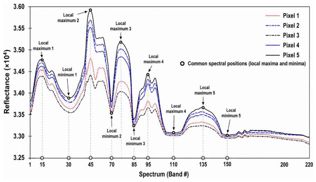
Figure 2.
Four types of abrupt signals processed by the wavelet bandpass filter ψ(t). Panels a-d show the four types of abrupt signals: upward maximum point, downward minimum point, protruding passing zero point, and concave passing zero point. Panels a’-d’ display the outputs of the four signals after applying the wavelet filter.
Figure 2.
Four types of abrupt signals processed by the wavelet bandpass filter ψ(t). Panels a-d show the four types of abrupt signals: upward maximum point, downward minimum point, protruding passing zero point, and concave passing zero point. Panels a’-d’ display the outputs of the four signals after applying the wavelet filter.
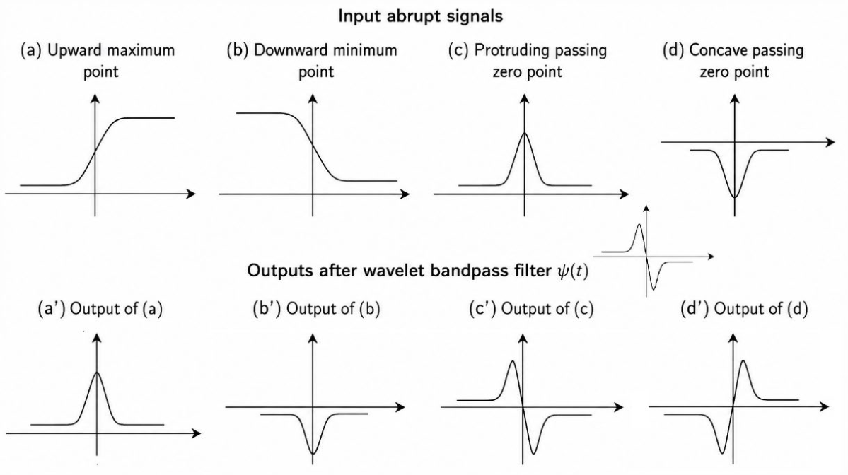
Figure 6.
Effect of on (a) class number and (b) time is investigated using WFGCA clustering with xstep=ystep=5, Tortho=0.8, and =5/7.
Figure 6.
Effect of on (a) class number and (b) time is investigated using WFGCA clustering with xstep=ystep=5, Tortho=0.8, and =5/7.
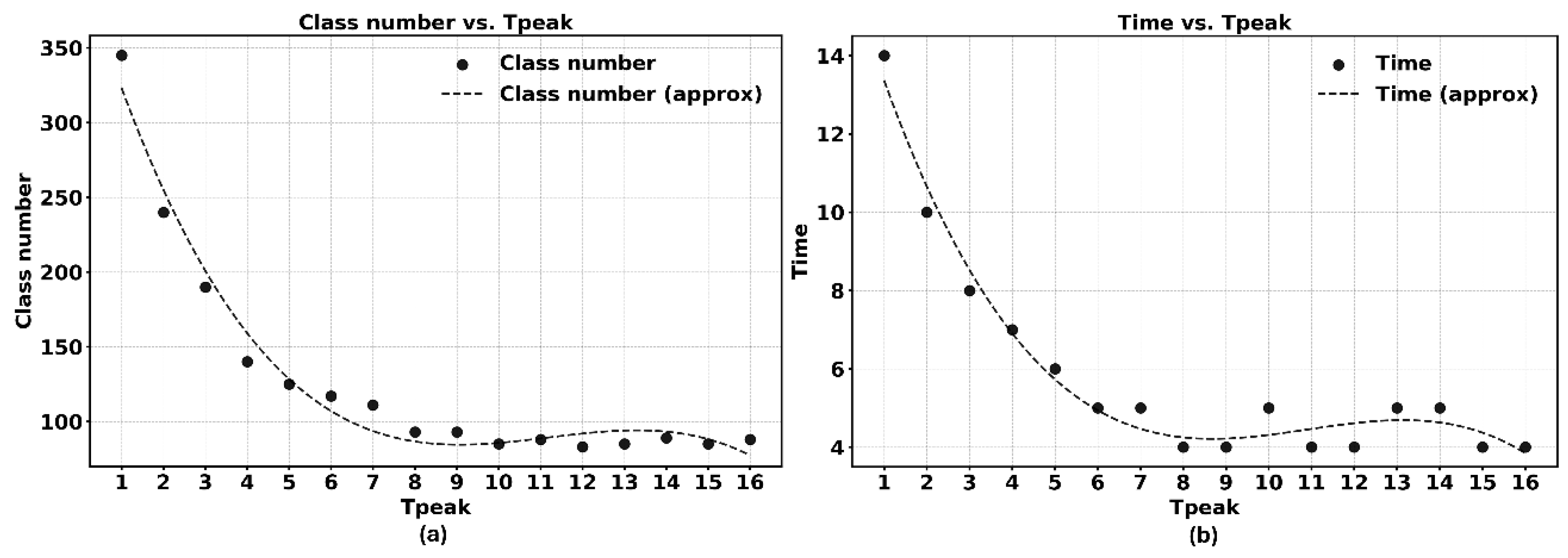
Figure 7.
Effect of on (a) class number and (b) time is investigated using WFGCA clustering with xstep=ystep=5, Tpeak=5, and =5/7.
Figure 7.
Effect of on (a) class number and (b) time is investigated using WFGCA clustering with xstep=ystep=5, Tpeak=5, and =5/7.
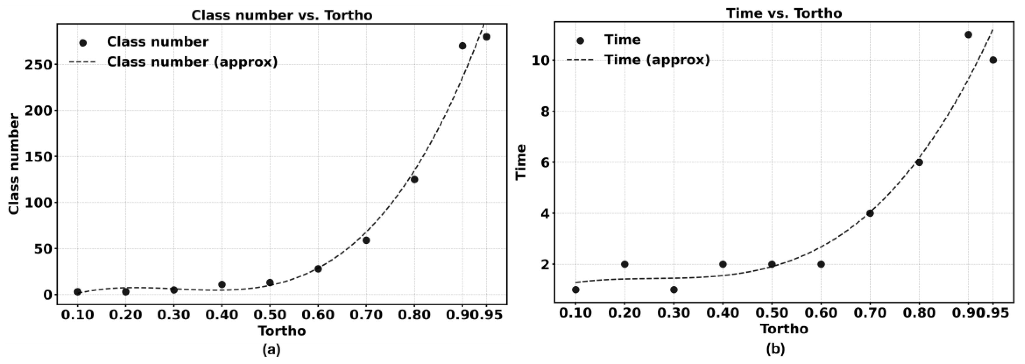
Figure 8.
Effect of on (a) class number and (b) time is investigated using WFGCA clustering with xstep=ystep=5, Tpeak=5, Tortho=0.8, and =7.
Figure 8.
Effect of on (a) class number and (b) time is investigated using WFGCA clustering with xstep=ystep=5, Tpeak=5, Tortho=0.8, and =7.
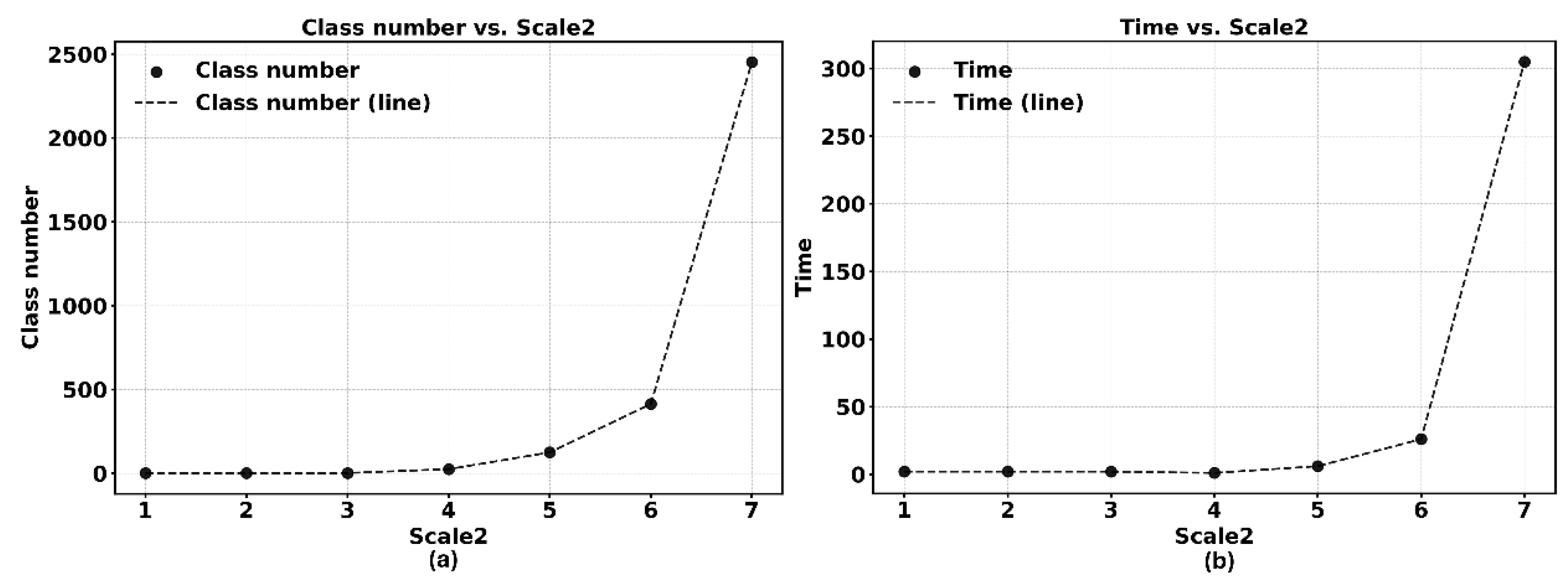
Table 1.
Sook Lake AVIRIS image: the effect of Tortho and Scale2 on WFGCA clustering (Sampling 5*5, Tpeak=5). Time unit is seconds.
Table 1.
Sook Lake AVIRIS image: the effect of Tortho and Scale2 on WFGCA clustering (Sampling 5*5, Tpeak=5). Time unit is seconds.
| Band no. | Tortho | Scale | Scale2 | Class no. | Time |
|---|---|---|---|---|---|
| 224 | 0.8 | 5 | 3 | 125 | 7 |
| 224 | 0.95 | 5 | 3 | 280 | 11 |
| 224 | 0.7 | 5 | 5 | 1488 | 183 |
Table 2.
Effect of with xstep=ystep, Tpeak=5, Tortho=0.8, and =5/7.
| Class number | Time | |
|---|---|---|
| 1 | 409 | 2652 |
| 2 | 272 | 112 |
| 3 | 194 | 26 |
| 4 | 168 | 10 |
| 5 | 125 | 6 |
| 6 | 112 | 5 |
| 7 | 100 | 4 |
| 8 | 103 | 4 |
| 9 | 82 | 4 |
| 10 | 81 | 3 |
| 11 | 73 | 3 |
| 12 | 64 | 3 |
| 13 | 56 | 3 |
| 14 | 71 | 3 |
| 15 | 51 | 3 |
| 16 | 57 | 2 |
| 17 | 44 | 2 |
| 18 | 45 | 3 |
| 19 | 51 | 3 |
| 20 | 44 | 2 |
Table 3.
Effect of with xstep=ystep=5, Tortho=0.8, and =5/7.
| Class number | Time | |
|---|---|---|
| 1 | 345 | 14 |
| 2 | 240 | 10 |
| 3 | 190 | 8 |
| 4 | 140 | 7 |
| 5 | 125 | 6 |
| 6 | 117 | 5 |
| 7 | 111 | 5 |
| 8 | 93 | 4 |
| 9 | 93 | 4 |
| 10 | 85 | 5 |
| 11 | 88 | 4 |
| 12 | 83 | 4 |
| 13 | 85 | 5 |
| 14 | 89 | 5 |
| 15 | 85 | 4 |
| 16 | 88 | 4 |
Table 4.
Effect of with xstep=ystep=5, Tpeak=5, and =5/7.
| Class number | Time | |
|---|---|---|
| 0.1 | 3 | 1 |
| 0.2 | 3 | 2 |
| 0.3 | 5 | 1 |
| 0.4 | 11 | 2 |
| 0.5 | 13 | 2 |
| 0.6 | 28 | 2 |
| 0.7 | 59 | 4 |
| 0.8 | 125 | 6 |
| 0.9 | 270 | 11 |
| 0.95 | 280 | 10 |
Disclaimer/Publisher’s Note: The statements, opinions and data contained in all publications are solely those of the individual author(s) and contributor(s) and not of MDPI and/or the editor(s). MDPI and/or the editor(s) disclaim responsibility for any injury to people or property resulting from any ideas, methods, instructions or products referred to in the content. |
© 2026 by the authors. Licensee MDPI, Basel, Switzerland. This article is an open access article distributed under the terms and conditions of the Creative Commons Attribution (CC BY) license (http://creativecommons.org/licenses/by/4.0/).
Copyright: This open access article is published under a Creative Commons CC BY 4.0 license, which permit the free download, distribution, and reuse, provided that the author and preprint are cited in any reuse.