

Submitted:
20 July 2026
Posted:
27 July 2026
You are already at the latest version
Abstract
The layer by layer 3D material deposition remains challenging when applied to complex Additive 3D-manufacturing material. Such process involve paste extrusion which surface geometry, density of layer and intrinsic properties must be very accurate whereas improper printing leads to porosity, irregular surfaces and may cause layers squeezing. When these cases occur, adjusting printing parameters is necessary. But, this also means a presence of human in the monitoring process surveilling printing in real time. Computer vision Systems at an early stage of their appearance, have been introduced for automate detection of cracks, irregular layer deposition, and texture inconsistencies, which directly affect structural integrity and print quality. They are later enhanced when deep learning and AI driven texture classification are directly introduced in their software framework. Additive manufacturing has then emerged, enabling the fabrication of complex geometries with high precision, but these techniques remain challenging when considering real time monitoring. This study proposes an advanced computer vision-based intelligent monitoring framework for real-time defect detection in extrusion-based 3D printing. Based on an hybrid Unet-VGG19 architecture, the proposed approach, combines the effectiveness of a strong semantic segmentation capability using the U-Net decoder, whose role is to perform upsampling the learned features discriminated by a powerful VGG19 encoder. To achieve better performance in the final model, the strategy of data augmentation is applied, leading to improving in generalization of the learned representations, even when transferred for a downstream tasks in non linear systems. A convergence investigation has also been detailed in the methodology and mathematical formulation section showing gradient stability and the model ability in identifying inter-layer boundaries and layer height variations under variable printing conditions. Our presented framework is employed to detect surface texture irregularities and local defects covering both concrete and soil-based materials. The aim is to present a complementary fine-tuned Unet-VGG-based classification, achieving better performance metrics than when evaluated on the dataset derived from Rodrigo Garcia Rill’s experimental works.In fact, experimental results demonstrate that the proposed hybrid architecture outperforms significantly the existing method, leading to superior performance scores when compared with the baseline published, previously trained on non augmented data. This results in a new transferable deep learning knowledge parameters, for printing tasks under extensive ground truth conditions, enabling scalable and real time defect monitoring across complex material systems and paving the way towards a robust quality control procedures in additive manufacturing.
Keywords:
AM (additive manufacturing)
; computer vision
; defect detection
; deep learning
; semantic segmentation
; 3D printing
I. Introduction
In modern industry of construction and structural engineering, paste-based materials are used for complex and highly customized geometries. Inappropriate fabricating tools can lead to strong waste in material. The mechanical performance and geometric fidelity of printed structures depend strongly on the stability of layer-by-layer deposition. The technology involved in this paper, is an end to end pipeline which aims to reduce these paste-waste from imperfect printing and enhance architecture flexibility.
Conventional quality control strategies, including manual inspection and contact-based sensing, are source of many problems: They lack to a post-process inspection providing corrective feedback during fabrication. Moreover, physical sensors may interfere with the fresh material during deposition. Theses two phenomena make conventional strategies unsuitable for real-time monitoring in extrusion-based additive manufacturing.
As a result, there is a strong need for non-destructive, and real-time monitoring systems, involving automated process, capable of detecting defects during the printing process. Addressing this challenge, recent advances in computer vision and artificial intelligence have opened new perspectives. The aim is to enable non-invasive, image-based monitoring of printed structures instead of classical image processing techniques.
This work proposes an advanced deep learning-based monitoring framework for defect detection in paste-based additive manufacturing. The proposed approach consists on mitigating two revolutionary techniques, resulting on a new hybrid U-VGG19 framework which combines a strong semantic segmentation U-Net tool with the hierarchical feature extraction power of the well known VGG19. The resulting model is further supported by data augmentation strategies during pre-processing and postprocessing morphological analysis to improve robustness under variable printing conditions.
The main contributions of this work are summarized as follows:
- An hybrid U-VGG19 architecture for robust defect segmentation which can be easily deployed in various paste-based materials.
- A computer vision pipeline , based on 3 FLIR Camera image data acquisition. for real-time monitoring of extrusion-based additive manufacturing processes.
- A robust mathematical analysis which combined with the data augmentation tool reinforce the gradient mechanism stability leading in a significant improvements over classical image processing and baseline deep learning models.
The remainder of this paper is organized as follows. Section II reviews related work in computer vision-based quality control for additive manufacturing. Section III describes the experimental setup, including the multi-camera system, materials, and data acquisition process. Section IV presents the proposed methodology and experimental results. Finally, Section V concludes the paper and discusses future research directions.
II. Related Works
Additive manufacturing of paste-based materials are applied in modern production of material layers, challenging the quality and high fidelity printers, but consistency and robustness is needed due to the intrinsic variability of material behavior during extrusion, deposition, and curing [1].
Computer vision and artificial intelligence have emerged as effective solutions for real-time monitoring and automated defect detection. This section reviews breakthroughs in quality control for paste-based additive manufacturing, focusing on vision-based monitoring systems, defect layer characterization, and deep learning approaches.
These approaches reduce reliance on manual inspection while improving robustness, scalability, and reliability in industrial environments.
A. Quality Control Challenges in Paste-Based Printing
Quality control remains a critical challenge in manufacturing processes involving extrudable paste-materials, for construction applications.
Considering 3D concrete printing (3DCP), (Buswell and al.) establishes a framework linking rheology process with geometrical parameters and material composition leading to a significant impact on the complex form performance in final structure. [2].
Although careful tuning of model parameters can achieve considerable system performance improvement, consistent results remains difficult and defect formation cannot be fully eliminated through parameter optimization alone. So that, real-time monitoring strategies have been increasingly investigated to detect anomalies during fabrication and reduce production failures.
Sensing methods, typically suffer from limited spatial resolution. Theses methods such as acoustic emission systems and photo-diode-based measurements are less effective for capturing geometric defects. In contrast, when vision-based approaches are applied in-situ for printing monitoring, including sensor working environment, they usually provide effective and richer spatial information with greater flexibility process [3,4].
B. Printing Strategies, Layer Pressing, and Defects in Paste-Based Additive Manufacturing
Recent studies focusing on extrusion-based 3D concrete printing, show the crucial role of printing strategies and their role in improving cementitious quality printing. Theses strategies include the layer pressing technique of the printed elements. Regarding the technique, a well-defined upper surface of the deposited layer being printed, may sometimes lead to a deformation in the underlying layers due to material squeezing. Consequently, printing velocity, and material flow rate becomes highly nonlinear and difficult to model using empirical approaches.
Experimental investigations have analyzed the influence of geometric and kinematic parameters on layer stability and shape evolution. They have been conducted to better understand these observed phenomena in extrusion-based 3D concrete printing. (Carneau2022) studies have focused on the effects of fresh concrete on the behavior of the extruded material under different printing conditions [5].
To summarize, we provide a list of some defects that commonly occur in paste-based 3D printing processes.Theses defects may induce deformation in the final printed components affecting consequently the structural and geometric quality.
- Cracks: They include the narrow break or split, typically caused by thermal stress, and can occur from insufficient inter-layer bonding, or material instability, damaging the structural integrity.
- Texture irregularities: they exhibit inconsistencies in shape and viscosity, resulting in a variation in the surface deposition and may result in both aesthetic and mechanical defect properties.
- Geometric deviations: show errors in layer height or improper alignment, in most case due to inappropriate extrusion control, leading to geometrical inaccuracies.
- Porosity: indicate the presence of air voids that may be captured during extrusion, this porosity may compromise material density and durability of the structure [6].
C. Computer Vision for Process Monitoring
Computer vision has emerged as the area of artificial intelligence challenging the non-destructive monitoring of additive manufacturing processes. The aim is to interpret the images or videos in a better way as done by human. Using depth sensing cameras, permits continuous observation when recording the process of material layer extrusion on real-time. The significant breakthrough needed is to include the detection of anomalies when captured to assess the extrusion based 3D printing without interrupting the process.
Compared to conventional manufacturing process based on cameras sensing systems, theses vision-based methods provide meaningful textural information, and high detailed spatial maps when their software provides deep learning and Artificial intelligence texture classification, making them particularly suitable for a wide variety of materials such as concrete [7].
D. Machine Learning and Deep Learning Methods
Machine learning can be summarized in three categories: Supervised, unsupervised or semi supervised learning. When labeled datasets are available, supervised learning methods are commonly used, in industrial inspection and additive manufacturing application. The two other approaches are applied for anomaly and manufacturing defects detection in cases where labeled or ground truth data are limited or unavailable.
In computer vision and manufacturing inspection process, the convolutional Neural Networks (CNNs), have accomplished competitive performance when considering image-based classification and segmentation tasks.
Comparing to other methods, they are widely integrated for computer vision-based system software adopted for visual inspection. These models automatically learn hierarchical feature representations from input raw data, bypassing manual feature engineering. Transfer learning has revolutionized machine learned models. In facts, even in the case of limited training data conditions, the learning knowledge can be reused and adapted to a new task, like defects detection. [8,9].
In the area of semantic segmentation architecture, SegNet and DeepLab have been widely applied for construction-related applications. The first approach is an encoder features extraction integrating a decoder which up-samples them for a pixel wise segmentation map, leading to surface defect analysis in additive manufacturing processes. Similarly, for this purpose of defect analysis , the second approach, known as an encoder backbone using atrous convolutions, have been also applied. Their later version also include an encoder decoder design. A comprehensive theoretical foundation of these methods can be found in [10]. This paper provides detailed coverage of deep learning architectures strategies, optimizations and training methodologies.
Beyond architectural developments, stability and convergence properties of learning systems have been investigated from a dynamical systems perspective, under nonlinear and delayed settings [11]. In this reference, sufficient conditions within a non linear framework, have been formulated to guarantee the stability and convergence behavior of neural models. In addition, theses published investigations show similarly the importance of stable optimization dynamics in ensuring reliable learning behavior and consistent model performance.
E. Recent Advances in the Literature
According to recent studies published, deep learning approaches have demonstrated affectiveness when applied for monitoring additive manufacturing processes. A CNN-based segmentation framework, build on hybrid U-net VGG19 architecture, has been recently deployed to extract inter-layer boundaries and analyze geometric variations in printed structures. This investigation is published in [12], by Rill-García et al.
In parallel, conventional texture analysis techniques have been widely used for surface quality classification; they are based on Local Binary Patterns (LBP) and Gray-Level Co-occurrence Matrices (GLCM) displaying. Such method is presented in [13], achieving robust performance in distinguishing localized defect levels.
Additionally, YOLO-based object detection framework, has revolutionary enhanced the effectiveness of deep learning models when applied for a real-time porosity and defects detection during 3D-Printing process, Li et al. [14]. YOLO is a single stage framework that has widely been integrated in computer-vision systems, enabling efficient and fast inference in continuous manufacturing environments as described by its original creator in the paper [15].
III. Methodology
A. Experimental Image Acquisition System
To evaluate the structural integrity, geometric compliance, and surface characteristics of paste-based 3D-printed specimens, a robust multi-camera vision framework was established. Subsequently, the reliability of defect detection procedure strongly depends on the physical ground truth parameters such as positioning, illumination stability, optical setting parameters and temporal synchronizing of the image sensing hardware.
The experimental framework ntegrates three FLIR Grasshopper3 (GS3-U3-41C6C) industrial cameras; known as high spatial resolution of pixels. They are also selected for their ability to capture fine surface topologies and capturing multi-scale structural irregularities. This study is applied through wide sensors configuration allowing diverse perspectives: such as focal lengths, kinematics or speed of material extrusion. The illustrated Figure 1. shows the operating framework used for collecting ground truth raw data illustrating the disposition of the 3 cameras used, and operational parameters are meticulously detailed in Table 1.
1. Sensor Distribution and Spatial Resolution
The deployment of the three specialized FLIR sensors is structured to cover complementary observation angles during the paste-based extrusion process:
- Camera A (Front-View): Operating from a stationary frontal perspective with a focal length of mm, it provides a medium field of view (FOV) to encapsulate the global 15 cm printed specimen. It primarily focuses on structural interlayer sizing (nominally 2 mm per layer) and macro-fissure propagation, operating at a spatial resolution of 73.2 m/pixel.
- Camera B (Nozzle-Mounted View): Dynamically attached to the print nozzle assembly at a well-defined orientation, this mobile sensor utilizes a mm lens. It enforces a narrow depth of field (4 cm) to achieve an ultra-high spatial resolution of 19.531 m/pixel, effectively isolating localized, micro-scale anomalies such as fine-scale porosities and small cracks (100–150 m) during material deposition.
- Camera C (Top-View): Positioned from a fixed top-down perspective using either a 12 mm or 25 mm focal length, this sensor monitors the newly deposited layer surfaces to audit surface-level porosities and textural irregularities down to 100–150 m.
B. Synchronization and Data Management Environment
To prevent temporal misalignment between separate image streams—which could introduce non-negligible artifacts and false positives during multi-view analysis—a strict synchronization and software workflow was established.
1. Software and Interfacing Architecture
The comprehensive software ecosystem is executed within a Python environment managed via Anaconda, ensuring stable dependency handling. Low-level camera interfacing and real-time parameters (including exposure time, gain, and frame rates) are controlled via the PySpin library, which wraps around the industrial FLIR Spinnaker SDK. Initial lens calibrations, optical alignments, and focal sharpness validations are pre-configured prior to active printing experiments using the FLIR SpinView utility.
High-resolution image preprocessing, tensor manipulations, and data analysis are handled utilizing the OpenCV, NumPy, Matplotlib, and Pillow libraries. Where available, hardware computational workloads are offloaded to CUDA acceleration cores to minimize processing bottlenecks during high-resolution multi-sensor image streaming.
2. Temporal Synchronization Protocol
A software-based synchronization protocol enforces simultaneous multi-device triggering. This simultaneous execution guarantees that all captured frames across Cameras A, B, and C correspond precisely to the identical physical stage of material extrusion, ensuring that any detected geometric variation is strictly caused by material rheology or print anomalies rather than inter-sensor acquisition delays. Each camera has its own sub-folder for the image records during operational runs, these uncompressed image sequences are continuously written into a structured directory. This data pipeline ensures consequently instantaneous pristine traceability for subsequent uncompressed multi-view dataset construction. Geometric error quantification, may be easily evaluated through mentioned saved sub-folder data, bypassing video complex compression techniques and giving rigorous adjustment geometric arrangement and camera calibration.
C. Dataset and Annotation Framework
To evaluate the capability of the proposed hybrid U-VGG19 semantic segmentation model, we propose a new benchmark based on the dataset derived from the study by Rill-García et al. [12].
This specialized dataset focuses on a fine-grained boundary extraction at pixel level within 3D-printed paste-based structural materials, specifically concrete and geomaterial (soil) mixtures. Some texture samples are presented in the Figure 2, presenting representative samples from the dataset used in this study. The illustration shows, a total of 16 images corresponding to four distinct classes: Fluid, Good, Dry, and Tearing. For samples are randomly shon for each class in order to highlight the variability of texture patterns within and across categories.
Figure 2.
Texture samples for the four classes (Fluid, Good, Dry, Tearing) across 16 test images.
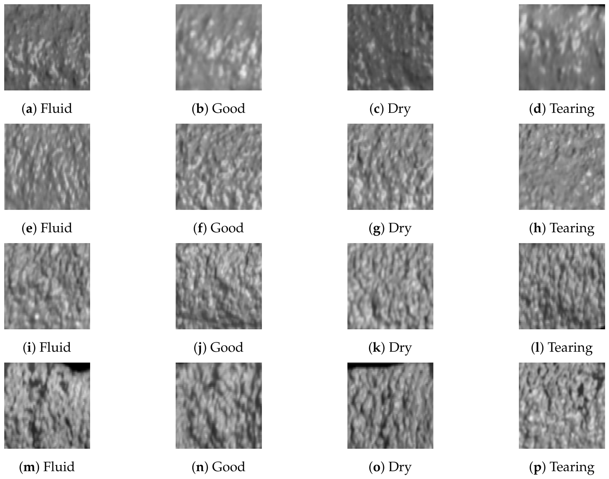
Figure 3.
Examples of data augmentation techniques applied to enrich the training dataset for 3D concrete printing layer monitoring.
Figure 3.
Examples of data augmentation techniques applied to enrich the training dataset for 3D concrete printing layer monitoring.
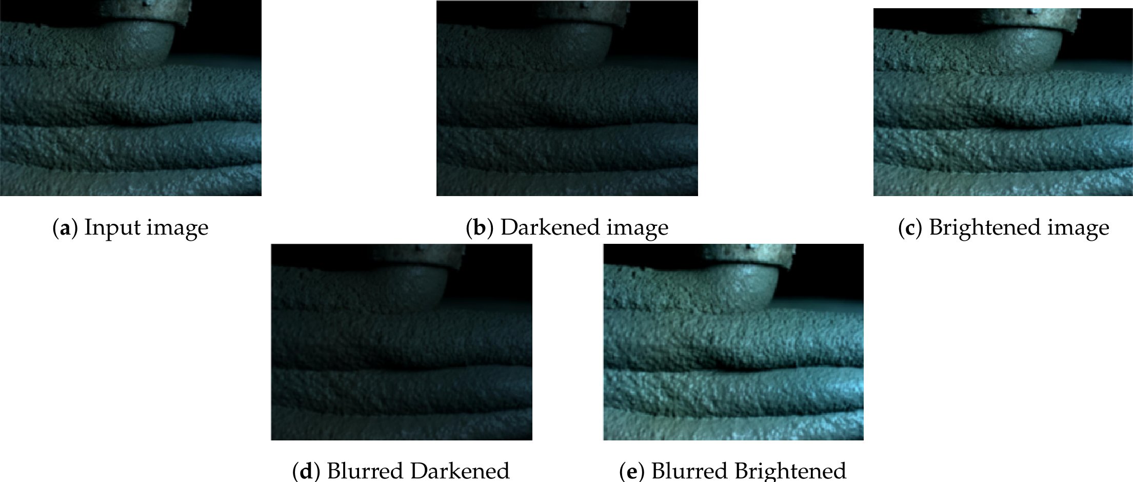
Figure 4.
Pixel-level dataset processing pipeline: from high-resolution raw camera acquisitions to paired training vectors.
Figure 4.
Pixel-level dataset processing pipeline: from high-resolution raw camera acquisitions to paired training vectors.

These visual examples exhibits a fined-qualitative overview of the raw data demonstrating some differences in surface characteristics between the considered classes.
Considering the Fluid class, Illustrations show smooth and continuous textures, while for the Good class they show well-formed and stable structures. In contrast, the four illustrations for the Dry class are characterized by rougher and more irregular patterns, whereas the visual Tearing class present discontinuities and structural defects.
Across this visualization step, we aim to better understand the nature of the data and support the effectiveness of the proposed classification strategy by emphasizing at an early stage of the involved pipeline, the discriminative boundary and texture features present in each class.
1. Data Characteristics and Patching Strategy
An original set which comprises 132 high-resolution ( pixels) RGB frames, was primarily selected to capture the printed layer geometries under varied optical illumination conditions.
for each frame a manually annotated ground-truth mask is introduced. These masks highlight the prominent interlayer boundaries, structural defects, and emphasize the relative texture variation.
A binary annotation encoding is applied for each frame: a series of a pixel value of 255 (white) denotes an interlayer joint interface, while a set of pixels with intensity value equal to 0 (black) isolates the structural material body and background.
Each pair of both image and its binary encoded mask is presented in a fixed format of pixels. This ensures limitation for consumed resources as computational memory allocation, and relative latency at each computational step.
Beyond structural standardization, this spatial attention strategy, increases discriminant local boundary exposure and fined-ground level partitioning, enhancing subsequently, the localized feature parsing capabilities of the U-Net contracting path.
2. Dataset Partitioning and Augmentation Protocol
Conventional split 80/20 distribution ratio is the applied during the preprocess setup; the extracted material patches are systematically segregated into independent subsets. The baseline partition yields consequently a training set encompassing core engineering samples and a validation set comprising 27 patches.
An optimal hyperparameter setting is strategically deployed to audit overfitting and verify generalization performance on unseen structural profiles.
To robustly train the deep network model and mitigate the impact of regularization under limiting constraints inherent to compact sample volumes, a multi-modal data augmentation strategy is introduced. The pipeline is executed exclusively on these training partitions. It scales the baseline training matrix by a structural multiplier of , thereby resulting on an expansion in the final operative training volume to frames. Consequently, we bring the total consolidated dataset size to 660 aligned images (including the training and validation subset).
This artificial expansion affects directly the network’s resilience against varying on-site operating environments. The different distinct transformation applied, are categorized into spatial, geometric and noise operations, as summarized in Table 2, with illustrative strategic steps of the resulting material detailed in Figure 3.
D. Experimental Setup and Data Acquisition Pipeline
The pipeline framework illustrated in Figure 4, downstreams from the baseline workflow, tracing the progression from raw multi-view captures to pair-aligned training matrices.
The system aims to monitor the dynamic extrusion behavior of 3D-printed cementitious and soil materials, deploying high-resolution FLIR industrial cameras.
The 3 cameras are strategically positioned, enabling real-time, multi-angle captures of the material bead morphology during printing and material extrusion.
The pipeline is therefor adjusted to ensure three continuous operational phases: first, a deterministic multi-camera calibration and hardware triggering, second a real-time synchronized multi-view frame ingestion, and third edge-to-cloud data streaming into a centralized repository for downstream deep learning segmentation and feature-driven classification analysis.
The pipeline is rigorously designed to ensure spatial and temporal consistency between all acquired views, captured by the three FLIR Cameras, which is essential for reliable defect detection and complex geometric analysis including intrinsic and extrinsic calibration parameters of printed layers.
The U-VGG19 model of Figure 5, is a hybrid semantic segmentation architecture that combines the feature extraction power of the VGG19 network with the reconstruction capabilities of the U-Net structure, as detailed in Table 3. This combination enables both rich hierarchical feature extraction and precise pixel-wise segmentation.
1. VGG19-Based Encoder
The encoder is based on the VGG19 network pre-trained on ImageNet. It consists of successive blocks of convolutional layers followed by ReLU activation functions and max-pooling operations.
At each spatial downsampling stage, the network:
- progressively reduces the spatial resolution of the input image,
- increases the depth of feature maps,
- extracts hierarchical representations ranging from low-level textures to high-level structural information.
Early layers capture simple patterns such as edges and gradients, while deeper layers extract more abstract features related to the geometry of printed layers.
2. U-Net Style Decoder
The decoder is symmetric to the encoder and aims to reconstruct a segmentation map with the same resolution as the input image.
It consists of:
- upsampling operations or transposed convolutions,
- successive convolution layers to refine segmentation results,
- gradual reduction of feature map depth.
This stage progressively restores spatial details lost during the encoding (downsampling) process.
3. Skip Connections
Skip connections link encoder and decoder layers at corresponding resolutions. These connections are basically set to concatenate feature maps from the encoder to the decoder.
They are essential for:
- preserving fine-grained spatial representations from the input information.
- recovering some details lost during the downsampling process.
- improving the boundary level segmentation accuracy.
The final output layer is a convolution followed by a sigmoid activation function, producing a pixel-wise probability map:
- : Then the corresponding pixel belongs to the inter-layer defect class,
- : Then the pixel is considered as belonging to the background.
4. Advantages of the U-VGG19 Architecture
The hybrid U-VGG19 framework synergistically combines, the ability of a pre-trained encoder backbone to accurate discriminant feature extraction driven by precise pixel-level localization inherent to the U-Net decoding pathway. This integration yields a highly robust semantic segmentation model, specifically tailored to isolate fined-grain micro-scale structural boundaries and complex geometric defects within 3D-printed cementitious and soil materials. Numerical stability, prevent excessive spatial over-parameterization, and maximize accurate boundary detection. The stability is strongly dependent to the operational layer parameters including the structural Max-Pooling 2D operations, specific spatial Dropout regularization rates.
The strategic optimization governed by the appropriate hyper-parameters are summarized in Table 4.
5. Fine-Tuning Optimization and Image Post-Processing
The proposed framework executes a dual-stage refinement process comprising structural network fine-tuning followed by algorithmic image post-processing. In this process, we convert inferences based on pixel-level semantic, into quantifiable engineering metrics. First, the network relies on a selective layer-freezing protocol, as comprehensively detailed in Table 5, leading to restricting the trainability of the foundational lower convolution layers.
the encoder successfully conserves the generic visual descriptors originally acquired from the Database. This encompasses visual edge hierarchies and basic textures.
Simultaneously, the network’s can actively adapt to the specific high-frequency surface maps native to 3D-printed cementitious and soil materials, by configuring the final six upper layers as fully trainable.
This specialized optimization drastically minimizes the native overfitting hazards brought on by the small engineering dataset volume.
Second, once raw segmentation maps are produced resulting from this optimized network, They are sent to a specific pipeline for post-processing. As outlined in Table 6,
This late-stage phase’s aims to extract clean geometric descriptors from the resulted segmented regions of interest, refine the initial binary matrices, removing high-frequency spatial distortions. These distortions may occur when changing in industrial illumination conditions vary.
This twofold optimization, which serves as a deterministic quality assurance checkpoint, ensures higher numerical precision during final dimensional tracking, making it possible to reliably locate and quantify interlayer anomalies inside the printed structures.
6. Classification Model Architecture
The following four classes: Fluid, Good, Dry, and Tearing, have to be miticulously identified by the classification model. The 532 texture features are computed from each image using Gray-Level Co-occurrence Matrices (GLCM) and Local Binary Patterns (LBP). These descriptors have the ability to capture both global and local texture information, providing a comprehensive representation of the image content.
The extracted features are then instantaneously reshaped into a tensor format meeting the requirements of the neural network. The two-dimensional convolutional layer, represents the first phase of this enrolled pipeline, it learns from the feature tensor and generates informative feature maps of the input data, highlighting their discriminative characteristics.
A Rectified Linear Unit (ReLU) is introduced as an activation function and applied after the convolution operation. ReLU improves the network’s ability to learn complex relationships between features while enhancing training efficiency, under non linear conditions.
A Dropout layer is subsequently incorporated as a regulation technique, to reduce overfitting by randomly ans temporarily deactivating a fraction of neurons during the training iteration, allowing all neurons to participate in learning over the course of training, thereby, improving the model ability to generalize to unseen data.
The resulting feature representations are then transferred to one or more fully connected (Dense) layers. These dense layers perform the final classification task combining the ability of the network to extract features and its capability to learn high-level decision boundaries between the different classes.
For this purpose a Softmax activation function is introduced. The network outputs are then transformed into normalized probability values. Concerning theses probability values, we aim to represent the likelihood that the input image belongs to a particular class. The highest probability is then selected as the final prediction.
The Adam (Adaptive Moment Estimation) optimizer, is than applied.
Its role is to adaptively adjust the learning rate according to the first and second moments of the gradients.
This optimization strategy ensures fast and stable convergence.
Furthermore, the class labels are encoded using the one-hot encoding technique, allowing efficient compatibility with the Softmax output layer and ensuring systematically a fast and efficient multiclass classification.
During inference, the same feature extraction procedure is applied to unseen images yielding to accurate and automated image classification based on texture characteristics.
In fact, the learned extracted feature tensor is fed into the trained network. The network uses the learned weights to identify the most likely class, based on the maximum probability among the classes.
7. Layer Dimension Analysis
Calculation of Absolute and Relative Layer Height
In 3D printing processes involving pasty materials, controlling the precision of the layer height is essential to guarantee the quality of the final part. Variations in layer thickness can lead to geometric defects such as waviness, deformations, or areas of structural weakness. The objective of this analysis is to calculate the absolute and relative height of the printed layers to identify these potential defects. The methodology is based on monitoring height variations and evaluating the error associated with each layer in order to correct or optimize the printing parameters.
Figure 6.
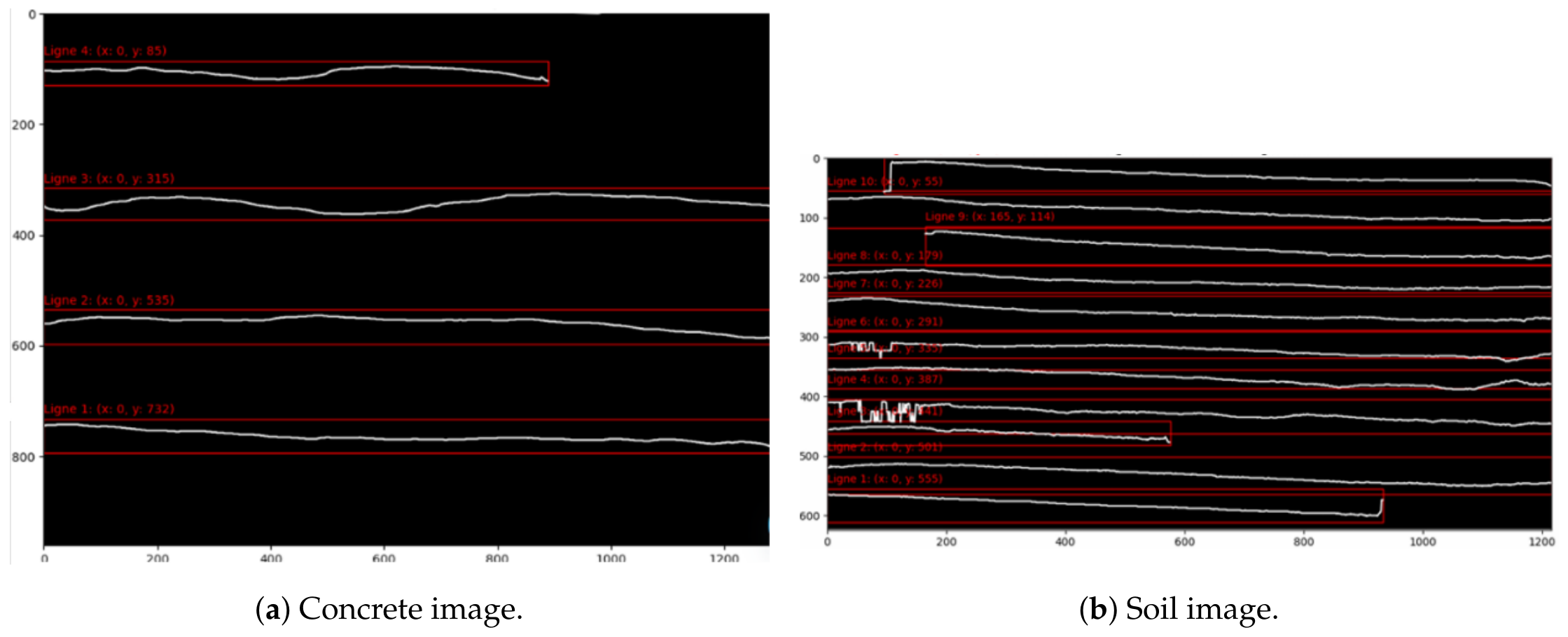
Comparison of detected lines and median traces for (a) concrete and (b) soil segmented images.
Figure 6.
Comparison of detected lines and median traces for (a) concrete and (b) soil segmented images.
To understand potential defects in 3D printing:
- Absolute height calculation: The absolute height of each layer is calculated relative to the base to measure height accumulation as the printing progresses. The absolute height is obtained by the following formula:where is the height of the i-th layer and is the theoretical thickness of each layer. This measurement serves to verify whether the height accumulation during printing complies with the initial specifications.
-
Absolute thickness error: The absolute thickness error corresponds to the deviation of this height with respect to the expected theoretical thickness, calculated by:This error allows for the identification of height discrepancies at each layer relative to the theoretical values.
-
Relative height: Relative height measures the height difference between two successive layers. It is calculated using the following equation:This measurement permits to localize fluctuations between successive layers, which may indicate inappropriate issues during the printing process.
-
Relative thickness error: is formulated to normalize, regardless of the layer scale, these differences and assess their effects. The relative thickness error is given by the following expression:This relative error is introduced to expresses the variation as a percentage, providing a standardized metric to assess printing stability across different layer scales.
-
Relative thickness error: The relative thickness error is expressed by:It evaluates the difference between the measured relative height and the theoretical thickness.
These height variation and thickness error curves, can be evaluated, through various plots, in the manufacturing process.
When calculated errors, provide problematic areas within the printed part. For instance if a positive error is detected this suggests an excessive accumulation of material, whereas a negative error may indicate a lack of material or an unintended compression of the layer. By analyzing these variations, we can adjust the printing parameters to improve the uniformity and quality of successive layers.
8. Texture Feature Extraction and Evaluation Metrics
The GLCM describes the frequency of occurrence of pairs of gray-level values at a predefined spatial relationship within an image.
Several statistical descriptors were computed from the co-occurrence matrix. Among the most representative features, the contrast quantifies local intensity variations.
The contrast formula is defined as:
where denotes the normalized probability of observing the gray-level pair .
The energy feature measures textural uniformity and is calculated as:
In addition, Local Binary Pattern (LBP) descriptors were employed to capture local micro-texture characteristics. The LBP operator assigns a binary code to each pixel according to the relative intensity of its neighboring pixels, its corresponding expression is given by the following:
where is the gray-level value of the central pixel, represents the gray-level value of the neighboring pixel, and the thresholding function is defined as:
The extracted texture descriptors were subsequently used as input features for the classification model.
E. Mathematical formulation for Performance Model Metrics
Evaluation of model performance depends on metrics, here is a breakdown of some evaluation metrics: At the beginning of this evaluation section, we provide a confusion matrix providing a tabular of model prediction in terms of true positives , true negative , representing class partitions, false positives and false negatives .
Precision measures the proportion of correctly predicted positive samples:
Recall quantifies the ability of the model to identify all relevant samples and is expressed by:
The F1-score is a powerful tool, since it combines Precision and Recall into a single performance indicator:
Finally, the Dice Similarity Coefficient (DSC) The Dice metric measures the overlap between the predicted segmentation and the ground truth. The Dice is used in the Loss function to emphasize robustness.
Dice provides a comprehensive measure of segmentation performance as it accounts for both false positives and false negatives.
1. Loss Function and Training Stability
The cross-Entropy or loss function, is defined as:
where! In this expression, N denotes the number of training samples, where as the class’s number is represented by C.
is the true label, whereas represents the predicted probability for class c.
In the following, the regularization term is used to mitigate overfitting and for generalization. It is therefore incorporated into the optimization objective.
The resulting loss function is then expressed as:
where M is the total number of trainable parameters, is the regularization coefficient governing the penalty strength, and represents the trainable network weights.
F. Combined Loss Function
They are often combined with cross-entropy as follows:
where is a weighting factor that balances the contribution of each loss term.
This combination helps improve:
- pixel-wise accuracy (cross-entropy loss),
- overlap quality between prediction and ground truth (Dice loss).
G. Adam Optimizer
The Adam optimizer (Adaptive Moment Estimation) updates network parameters using adaptive estimates of first and second moments of the gradients.
The first moment estimate is defined as:
The second moment estimate is given by:
Bias-corrected estimates are computed as:
The parameter update rule is:
where is the learning rate, and are decay rates, and is a small constant for numerical stability. Several optimization techniques were used to guarantee steady gradient propagation and strong convergence throughout training. To lessen co-adaptation between neurons and enhance model generalization, dropout regularization at a multiple rate was used.
Furthermore, the Adam optimizer was used with a learning rate. Throughout the training process, Adam reduces gradient oscillations, speeds up convergence, and improves numerical stability by adaptively updating network parameters using estimates of the first and second moments of the gradients. When combined, these methods enhance generalization performance and optimization robustness, especially when training on comparatively small datasets.
IV. Results and Discussion
We begin first to analyze the published references dressed in the Table 7.
Deep learning-based frameworks [3,4,8,9,10,12,15] greatly outperform previous published approaches in additive manufacturing applications.
Due to their reliance on indirect physical signal collecting techniques or handmade feature engineering [13], early approaches show a limited capacity to capture fine-grained spatial patterns. These include physical measurements taken from extrusion-based additive manufacturing processes [2], process signal-driven defect detection techniques in laser powder bed fusion (LPBF) systems [4], acoustic emission-based monitoring strategies [3], and conventional industrial inspection frameworks based on indirect sensing modalities and classical measurement protocols [6]. When taken as a whole, these approaches are limited in their ability to represent intricate spatial structures and minute local fluctuations in the underlying data due to their dependence on indirect observables and manually created descriptors.
Convolutional neural network-based methods has shown better detection performance, but they remain sensitive to illumination variations, noise, and domain shift, which can degrade their robustness in real operational environments.
A. Qualitative and Quantitative Performance Analysis
To evaluate the reliability of the dataset trained using BLP and GLCM-based feature extraction, and to assess the capability of the proposed camera system in capturing texture variations, Figure 7 presents the four concrete texture classes used for validation. In addition, Figure 8 illustrates the model predictions on two clay texture classes acquired using the FLIR camera, demonstrating its ability to generalize across different material types.
Results for improved extrusion layer segmentation are further, presented and discussed, for both concrete and soil extrusion acquired using our FLIR camera-based acquisition system.
Although the proposed method based on BLP and GLCM features achieves very strong performance, we introduce an improved approach based on a U-Net architecture combined with a VGG backbone to further enhance feature representation and segmentation accuracy.
Specifically, the encoder blocks progressively reduce the spatial dimensions of the input tensors in order to capture deep contextual cues associated with interlayer boundary profiles in 3D-printed materials. Conversely, the decoder pathway reconstructs pixel-wise segmentation maps through successive transposed convolutions, combined with feature fusion from the corresponding encoder stages. These skip connections play a crucial role in preserving edge sharpness and boundary details, which are essential for isolating micro-scale defects along the highly complex layered extrusions.
Moreover, a qualitative study, introduced in Section E, based on the segmented mask was conducted. The results show that the baseline suffers from a high rate of false positives introduced by environmental noise. The improved model output achieves better clean, of theses false values, demonstrating its operational readiness for closed-loop quality control applications.
This substantial qualitative improvement is directly rooted in the structural layout of the network. In fact, Dice loss is employed to handle class imbalance by directly optimizing the overlap between predicted and reference masks, Equ. (16). The network’s hyperparameters, were rigorously calibrated in purpose to optimize classification performance while ensuring stability during backpropagation. Our improved model based on U-VGG19 seamlessly integrates the deep hierarchical feature extraction capabilities combined with the precise spatial reconstruction properties inherent to the U-Net decoder loop. This cohesive design framework enables the network to learn, high-level semantic representations while concurrently preserving fine-grained localized spatial coordinates.
The VGG19 encoder has the ability of capturing the VGG19 deep features generating huge number of parameters. The introduction of the next GlobalAveragePooling2D ensures an efficient dimensionality reduction mechanism since it reduces the total parameter count compared to conventional flattening methods. This mechanism results in lowering the computational complexity while reduction the network’s susceptibility to spatial translations.
The intermediate dense hidden layer is configured to provide sufficient non-linear capacity to decode the high-dimensional vectors passed by the convolutional backbone, it is regularizated via the weight decay and is followed by the Dropout layer configured at a strict rate of the selected value 0.5.
This choice aims to prevent the model from overfitting to structural noise.
By randomly deactivating half of the neural pathways during each training forward-pass, the network is encouraged to learn more robust and less co-adapted feature representations, significantly mitigating the risk of overfitting.
Additionally, a Softmax function was used to activate the output 4 nodes, resulting in a well-calibrated probability distribution across the intended structural categories (Fluid, Good, Dry, and Tearing).
Concerning the optimization strategy, we first adopt a learning rate baseline of 0.0001. to achieve a trade off between fast convergence and gradient stability.
The Adam optimizer was selected due to its computational efficiency and its efficiency. In fact, it learns adaptive momentum and captures the velocity like the behaviour of the gradient.
It has the ability to train the network for the four classes learning individual parameters, by minimizing the sparse_categorical_crossentropy loss function.
The layer-freezing configuration was precisely adjusted across the pre-trained VGG19 backbone.
Considering, the implementation of the presented U-VGG19 architecture, the standard Keras deep learning framework comprises 22 layers, including convolutional blocks and intermediate max-pooling operations.
Under the proposed fine-tuning strategy, the first 16 layers of the network were strictly frozen (layer.trainable = False), while only the final 6 upper layers were permitted to remain trainable (layer.trainable = True).
The 16 Locked layers are used as static general-purpose feature extractor. Since they have been trained on the large-scale ImageNet repository, they can easily work as filters able to detect visual primitives, basic contours, elemental textures...Their weights are locked ensuring that theses essential representations are protected from forgetting.
Consequently, this selective freezing strategy reduces the number of trainable parameters, improves computational efficiency during backpropagation, and mitigates overfitting on the target dataset.
Discussion the Practical Results
The ablation experiment section highlights the dependency of the model on the data augmentation strategy integrated in the pipeline. We show that the absence of data augmentation leads to a noticeable degradation in Dice score on the test set, resulting in reducing the ability of the model to generalize across various condition constraint in the operating world. In the opposite case, the use of data augmentation enriches the training distribution, and results in better Dice scores.
As outlined in Table 8, augmentation data improves robustness and enhances generalization performance on unseen samples.
These findings confirm the importance of augmentation strategies in segmentation tasks for ensuring stability and predictive reliability.
Figure 9 illustrates the training convergence behavior of the proposed model over successive epochs. The loss curve exhibits a steady decrease, indicating stable optimization throughout training.
A limited gap between training and validation curves is observed, suggesting that the network does not suffer from severe overfitting, this behavior is also supported by the combined effects of data augmentation and dropout regularization.
During evaluation on the raw testing set, the improvement appears less pronounced, suggesting that although data augmentation significantly enhances generalization, the inherent variability of the dataset remains a limiting factor.
Nevertheless, the F1-score results reported in Figure 10 demonstrate consistently accurate performance across the four extrusion classes, confirming that the proposed improved U-VGG19 classification model effectively discriminates between different extrusion states under realistic conditions.
While the classification results confirm the effectiveness of the proposed model, the overall pipeline performance also depends on the quality of the input data used for segmentation. The primary goal of the artifact removal preprocessing step was to prepare the input images for optimal feature extraction by the deep segmentation network. As visually evidenced in Figure 11 and Figure 12, the proposed method effectively suppresses visual disturbances commonly encountered in construction environments, including illumination artifacts, sensor noise, and extraneous shadows from surrounding equipment, while preserving the semantic integrity of critical layer boundaries.
Comparisons before and after artifact removal are illustrated in Figure 12a,c for the concrete dataset, and in Figure 12b,d for the soil dataset. This preprocessing step results in a clearer delineation between cement paste and aggregates within the bead profile and reduces ambiguities caused by heterogeneous surface textures and micro-shadowing effects. By standardizing the visual domain across different materials, it significantly contributes to improved segmentation performance on unseen validation data.
Following the segmentation stage, a geometric post-processing step is applied to extract structural information from the predicted masks. To quantitatively assess the accuracy of the reconstructed geometry, the evaluation is based on the error metrics defined in the Methodology section, Section 7, namely the absolute error and relative error. The detected lines and their corresponding medial traces extracted from the segmented concrete image are illustrated in Figure 13.
Across these steps, the robustness of the proposed approach is consistently validated on both the concrete and soil materials.
Although the model was originally trained on concrete extrusion data, These findings suggest that basic aspects of extrusion behavior are captured by the learned feature representations. The model can be readily continue to be applied to various materials. This demonstrates the potential applicability of the proposed approach to real-world for various materials in additive manufacturing environments.
B. Training Stability and Robustness Analysis
The stability of learning-based models in additive manufacturing remains a critical challenge, particularly under perturbations such as noise, illumination variations, and domain shifts. Prior studies have shown that neural network performance can be sensitive to input perturbations and training dynamics [8,10,11]. In addition, instability issues related to feature extraction and representation learning have been widely observed in practical deep learning systems applied to industrial monitoring tasks [3,4,9].
In our case, the smooth convergence of the loss function, together with the limited gap between training and validation curves, indicates a well-conditioned optimization process.
This behavior suggests stable gradient propagation, supported by the combined effect of skip connections, data augmentation, and artifact removal preprocessing.
From a mathematical perspective, the stability of the optimization process can be interpreted through the convergence behavior of the loss function:
where the training loss approaches converge to a stable equilibrium without showing oscillations.
The stable gradient propagation is ensured by bounded gradient updates during backpropagation:
This, especially in deep encoder-decoder systems, helps reduce exploding gradient issues.
Additionally, the slight difference between test and training performance can be used to represent the model’s generalization behavior:
highlighting the ability of the model to maintain consistent performance on unseen data.
In addition, the model demonstrates robustness under input variability, maintaining consistent prediction behavior even in the presence of noise, texture heterogeneity, and illumination variations. This robustness can be interpreted through invariance to small perturbations in the input space:
reflecting a form of implicit stress resilience and reinforcing the reliability of the proposed architecture xhen deployed in realistic operational environments.
where denotes the nonlinear mapping learned by the proposed U-Net–VGG19 architecture, which transforms an input optical image into its corresponding predicted segmentation mask .
The perturbation represents a small variation in the input image.
It can occur due to the real world constraints such as illumination fluctuations, sensor noise, or slight spatial translations.
The condition indicates that the perturbation has a negligible magnitude. Consequently, the relation implies that the network generates nearly identical segmentation outputs despite these minor perturbations, thereby demonstrating robustness and stability under realistic imaging conditions. This observation is consistent with prior studies on the sensitivity and robustness of deep neural networks to input perturbations and domain shifts [8,9,10,11]. In industrial additive manufacturing applications, similar instability issues have been reported due to sensor noise and environmental variations [3,4].
C. Integration into Closed-Loop Additive Manufacturing Systems
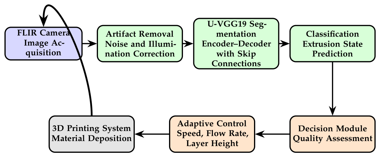
The proposed framework is designed for integration into closed-loop additive manufacturing systems, enabling real-time monitoring and feedback control during the extrusion process. By combining fast inference with reliable segmentation and classification outputs, the model provides continuous assessment of extrusion quality at each printing stage, as illustrated in Figure 14.
This real-time capability allows the system to detect deviations in layer formation and material behavior, which are then translated into control signals to adjust process parameters such as extrusion speed, flow rate, and layer height. As shown in the proposed architecture, the decision module acts as an intermediary between the perception stage (image acquisition, artifact removal, and deep feature extraction) and the control stage responsible for actuation of the 3D printer.
As a result, the framework supports adaptive control strategies aimed at improving print quality and reducing defect propagation during fabrication. The stability of the model predictions and its robustness to input variability further reinforce its suitability for deployment in industrial environments requiring continuous and automated decision-making.
Recent studies have demonstrated the effectiveness of integrating in-situ monitoring with feedback control for additive manufacturing applications, where sensor or vision-based information is used to dynamically regulate printing conditions [2,12]. In particular, vision-based and sensor-driven monitoring approaches provide the necessary feedback signals for adaptive correction mechanisms, contributing to improved process robustness under variable operational conditions [3,4].
Figure 11.
Comparison of segmentation results: original FLIR image, initial model output, and improved model output after architectural enhancements.
Figure 11.
Comparison of segmentation results: original FLIR image, initial model output, and improved model output after architectural enhancements.
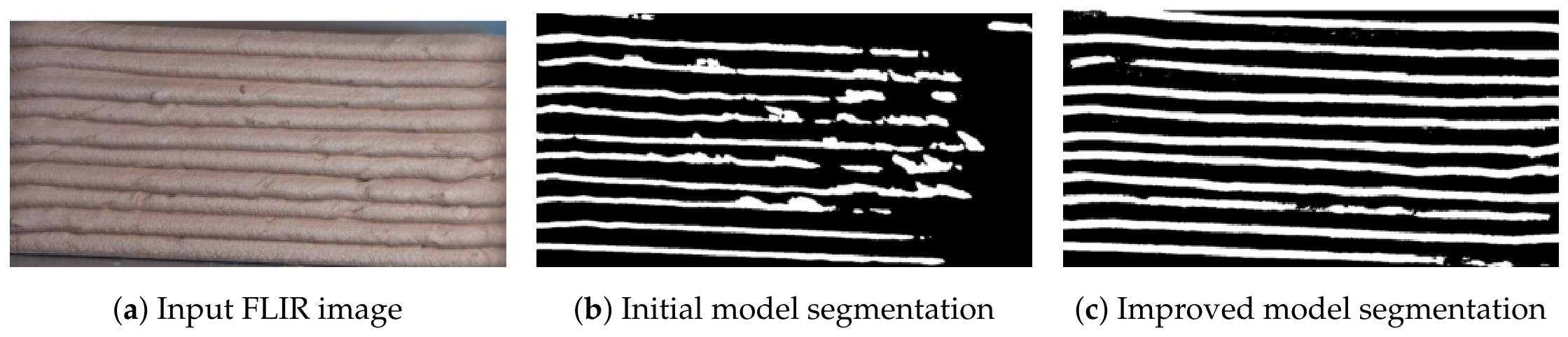
Figure 12.
Comparison of images before and after artifact removal for concrete and soil datasets. Concrete results are shown on the left, while soil results are shown on the right.
Figure 12.
Comparison of images before and after artifact removal for concrete and soil datasets. Concrete results are shown on the left, while soil results are shown on the right.
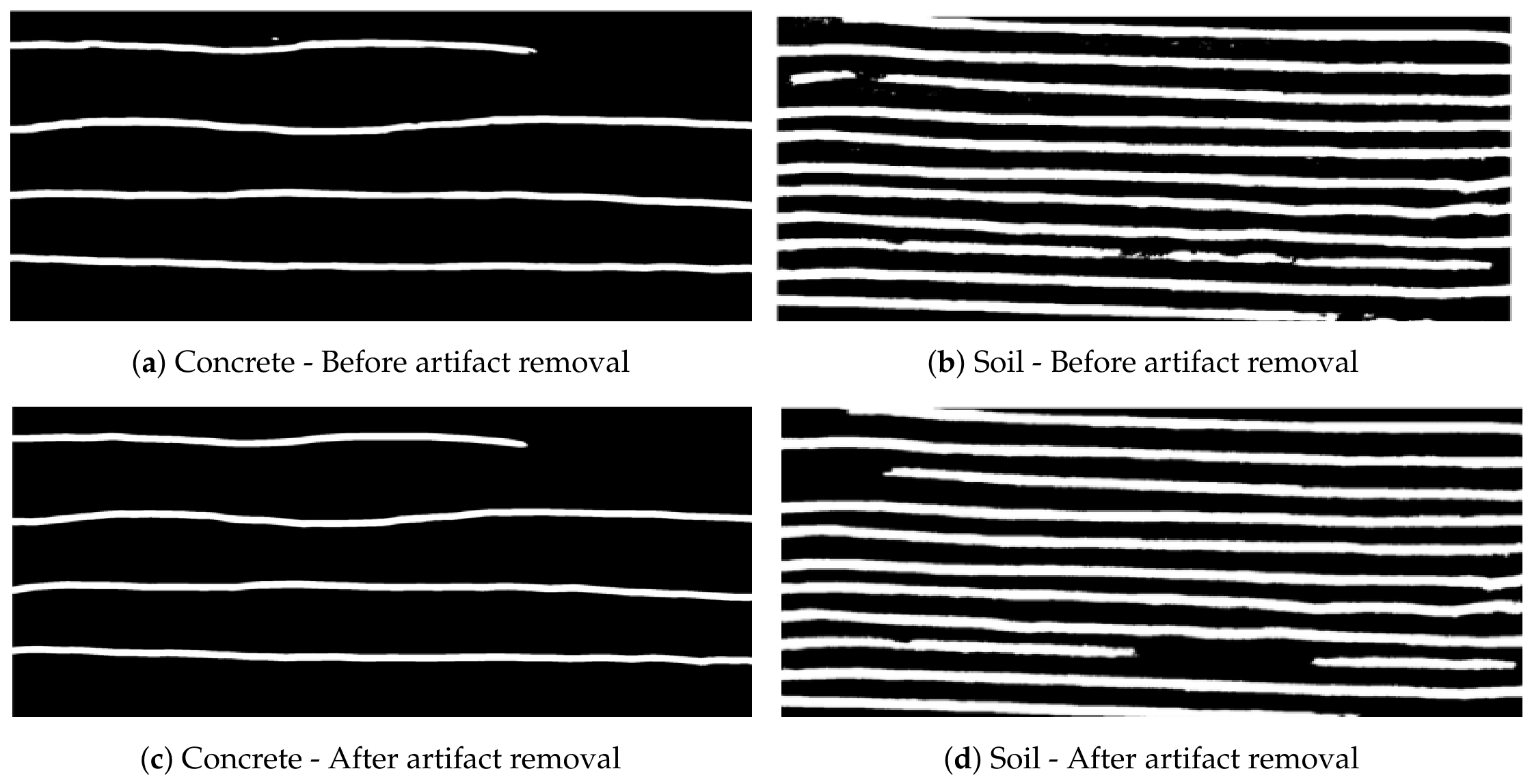
Figure 13.
Ground truth thickness distribution of the material sample.
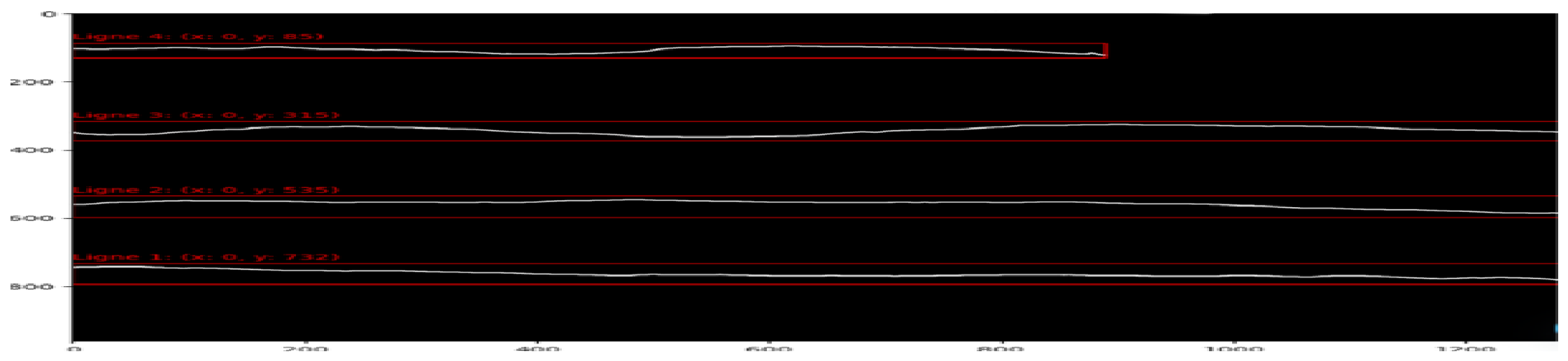
Figure 14.
Improved closed-loop control architecture for real-time monitoring and adaptive control in additive manufacturing systems.
Figure 14.
Improved closed-loop control architecture for real-time monitoring and adaptive control in additive manufacturing systems.
V. Conclusion
This study successfully developed and validated a hybrid U–VGG19 architecture designed for real-time defect segmentation and classification in multi-material 3D printing applications. By effectively combining deep semantic encoding with fine-grained spatial information through skip connections, the proposed framework demonstrates strong robustness and adaptability to the complex and heterogeneous surface textures characteristic of both cementitious and soil materials.
Experimental results further show that the incorporation of targeted data augmentation and artifact removal preprocessing greatly improves the model’s generalization capability,
By an ablation study vs augmentation strategy, We also show how our improved UNet-VGG19 model, achieves superior performance across all evaluation metrics, compared to the baseline introduced by [12]. Since the Dice loss has the ability to optimize the overlap between predicted and ground truth positives. It is introduced in the cross-entropy function (loss), improving performance on imbalanced datasets. This makes the model more able to generalize to unseen data. In fact, existing methods are very sensitive to noise illumination factors, and other perturbations in the real word. The section introduced to discuss the gradient stability shows how our framework improves robustness to input perturbations making it more stable and how it is more reliable to feature representations under noisy conditions.
Overall, this work bridges the gap between laboratory-based computer vision approaches and practical quality control in additive manufacturing. Beyond segmentation and classification, the proposed framework establishes the foundations for intelligent monitoring systems capable of supporting autonomous manufacturing operations. The integration of image acquisition, artefact removal, deep feature extraction, and decision-making modules demonstrates the feasibility of a closed-loop quality control strategy for additive manufacturing processes.
Building on these results, future developments could extend the proposed framework toward real-time monitoring and adaptive process control. In particular, the system could be extended to an online inference pipeline capable of processing streaming data from FLIR cameras, ensuring immediate detection of structural anomalies during fabrication. Furthermore, coupling the vision system with robotic control modules would enable closed-loop feedback mechanisms, allowing automatic adjustment of extrusion parameters such as printing speed, material flow rate, and layer height in response to detected defects. Such developments would represent an important step toward fully autonomous and self-correcting additive manufacturing systems.
AI Disclosure Statement
During the preparation of this report, I used AI TOOL in order to review basic checks Grammar and Spelling. After using this tool, I reviewed and edited the content as needed and I take full responsibility for its content.
Acknowledgments
The authors would like to express their sincere gratitude to the members and technical staff of the Numerical Sciences Laboratoiry of Nantes (LS2N) for their valuable support, insights, and collaborative research environment. We are particularly grateful for the computational resources and the specialized imaging equipment, including the FLIR cameras provided by the laboratory, which were essential for the data collection and successful validation of this work.
References
- Berchon, M.; Luyt, B. L. L’impression 3D; Editions Eyrolles, 2014. [Google Scholar]
- Buswell, R. A.; et al. 3D printing using concrete extrusion: A roadmap for research. Cem. Concr. Res. 2018, vol. 112. [Google Scholar]
- Shevchik, S. A.; et al. Acoustic emission for in situ quality monitoring in additive manufacturing using spectral convolutional neural networks. Addit. Manuf. 2018, vol. 21. [Google Scholar]
- Okaro, I. A.; et al. Automatic fault detection for laser powder-bed fusion using semi-supervised machine learning. Addit. Manuf. 2019, vol. 27. [Google Scholar]
- Carneau, P.; et al. Layer pressing in concrete extrusion-based 3D-printing: Experiments and analysis. Cem. Concr. Res. 2022, vol. 155. [Google Scholar]
- Scholz-Reiter, B.; Weimer, D.; Thamer, H. Automated surface inspection of cold-formed micro-parts. CIRP Ann. 2012, vol. 61. [Google Scholar]
- Oleff, A.; et al. Process monitoring for material extrusion additive manufacturing: A state-of-the-art review. In Progress in Additive Manufacturing; 2021. [Google Scholar]
- Krizhevsky, A.; Sutskever, I.; Hinton, G. E. ImageNet classification with deep convolutional neural networks. NeurIPS 2012. [Google Scholar] [CrossRef]
- Weiss, K.; Khoshgoftaar, T. M.; Wang, D. A survey of transfer learning. J. Big Data 2016. [Google Scholar] [CrossRef]
- Goodfellow, I.; Bengio, Y.; Courville, A. Deep Learning; MIT Press, 2016; Available online: https://www.deeplearningbook.org/.
- Guo, Y.; Ge, S. S.; Arbi, A. Stability of Traveling Waves Solutions for Nonlinear Cellular Neural Networks with Distributed Delays. J. Syst. Sci. Complex. Available. 2022, vol. 35, 18–31. [Google Scholar] [CrossRef]
- Rill-García, R.; Dokladalova, E.; Dokladal, P.; Charrier, M.; et al. Inline monitoring of 3D concrete printing using computer vision. Addit. Manuf. 2022, vol. 60, 103175. [Google Scholar] [CrossRef]
- Szeliski, R. Szeliski, Computer Vision: Algorithms and Applications; Springer, 2022; Available online: https://szeliski.org/Book/.
- Li, Y.; Mu, H.; Polden, J.; Li, H.; Wang, L.; Xia, C.; Pan, Z. Towards intelligent monitoring system in wire arc additive manufacturing: a surface anomaly detector on a small dataset. Int. J. Adv. Manuf. Technol. Available. 2022, vol. 120(no. 7–8), 5225–5242. [Google Scholar] [CrossRef]
- Redmon, J.; et al. “You Only Look Once: Unified, real-time object detection,” in CVPR. 2016. Available online: https://arxiv.org/abs/1506.02640.
Figure 1.
Experimental setup showcasing the strategic positioning and perspective distribution of the three FLIR industrial cameras around the robotic 3D printing platform for multi-view defect monitoring.
Figure 1.
Experimental setup showcasing the strategic positioning and perspective distribution of the three FLIR industrial cameras around the robotic 3D printing platform for multi-view defect monitoring.
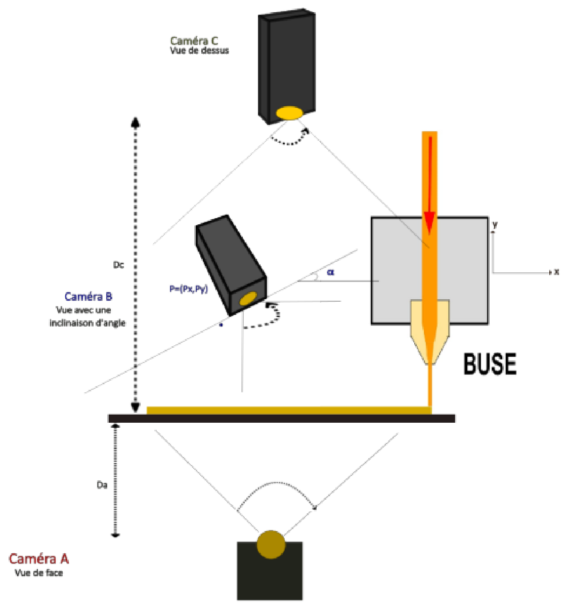
Figure 5.
U-VGG19 encoder-decoder architecture with dropout regularization for inter-layer defect segmentation in 3D-printed materials.
Figure 5.
U-VGG19 encoder-decoder architecture with dropout regularization for inter-layer defect segmentation in 3D-printed materials.
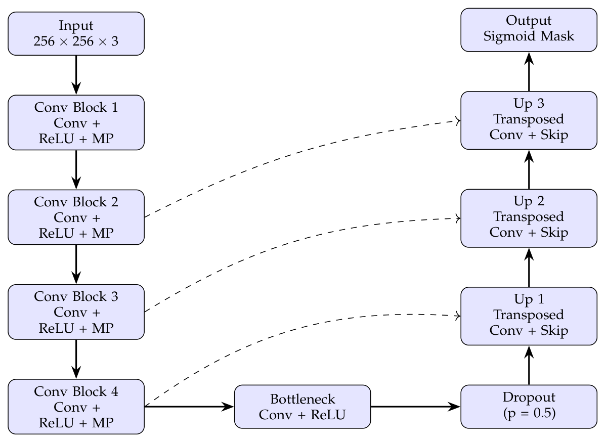
Figure 7.
Prediction results for the four classes with associated confidence probabilities obtained from the proposed classification model.
Figure 7.
Prediction results for the four classes with associated confidence probabilities obtained from the proposed classification model.
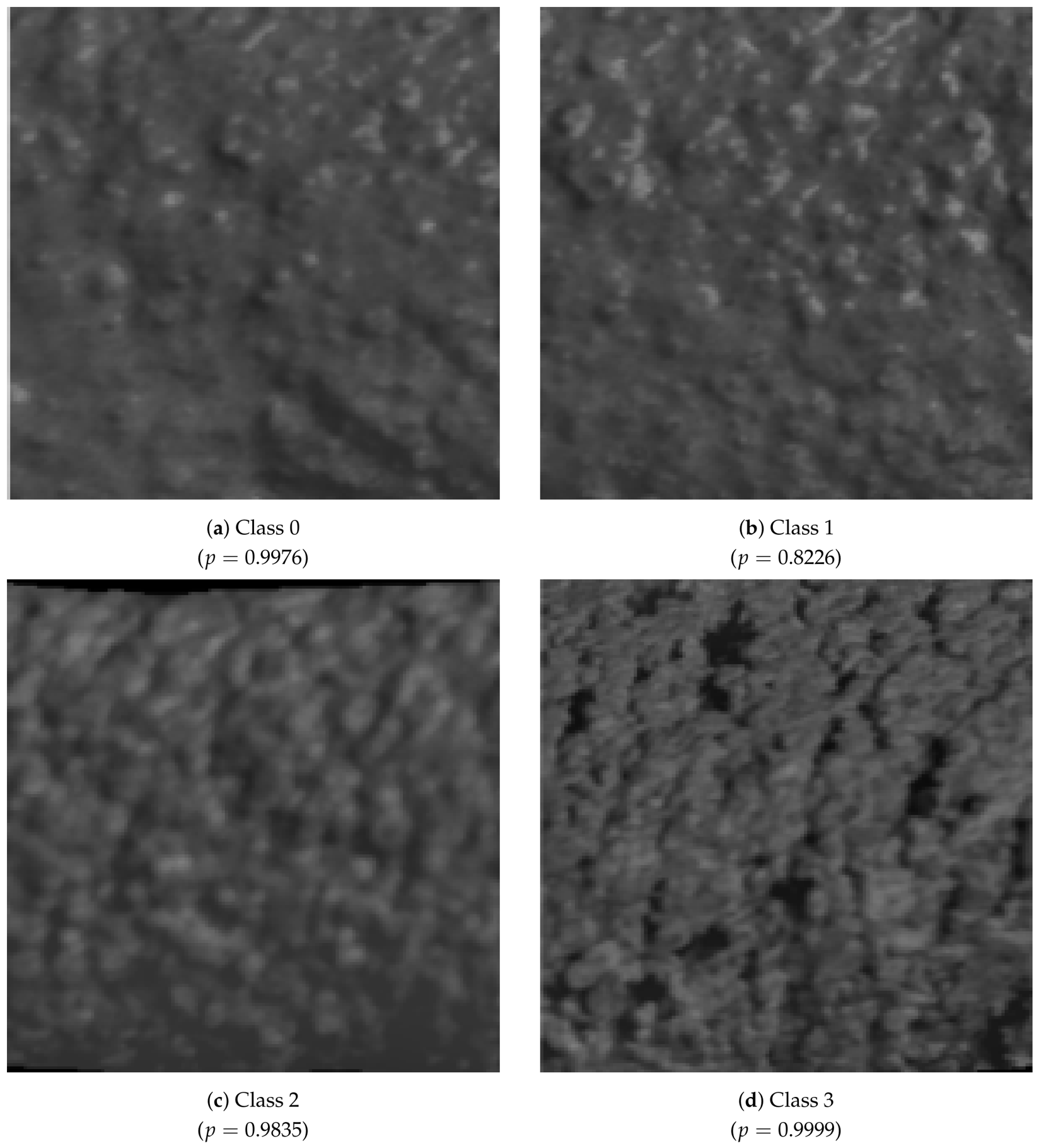
Figure 8.
Prediction results on FLIR thermal images using the proposed classification model.
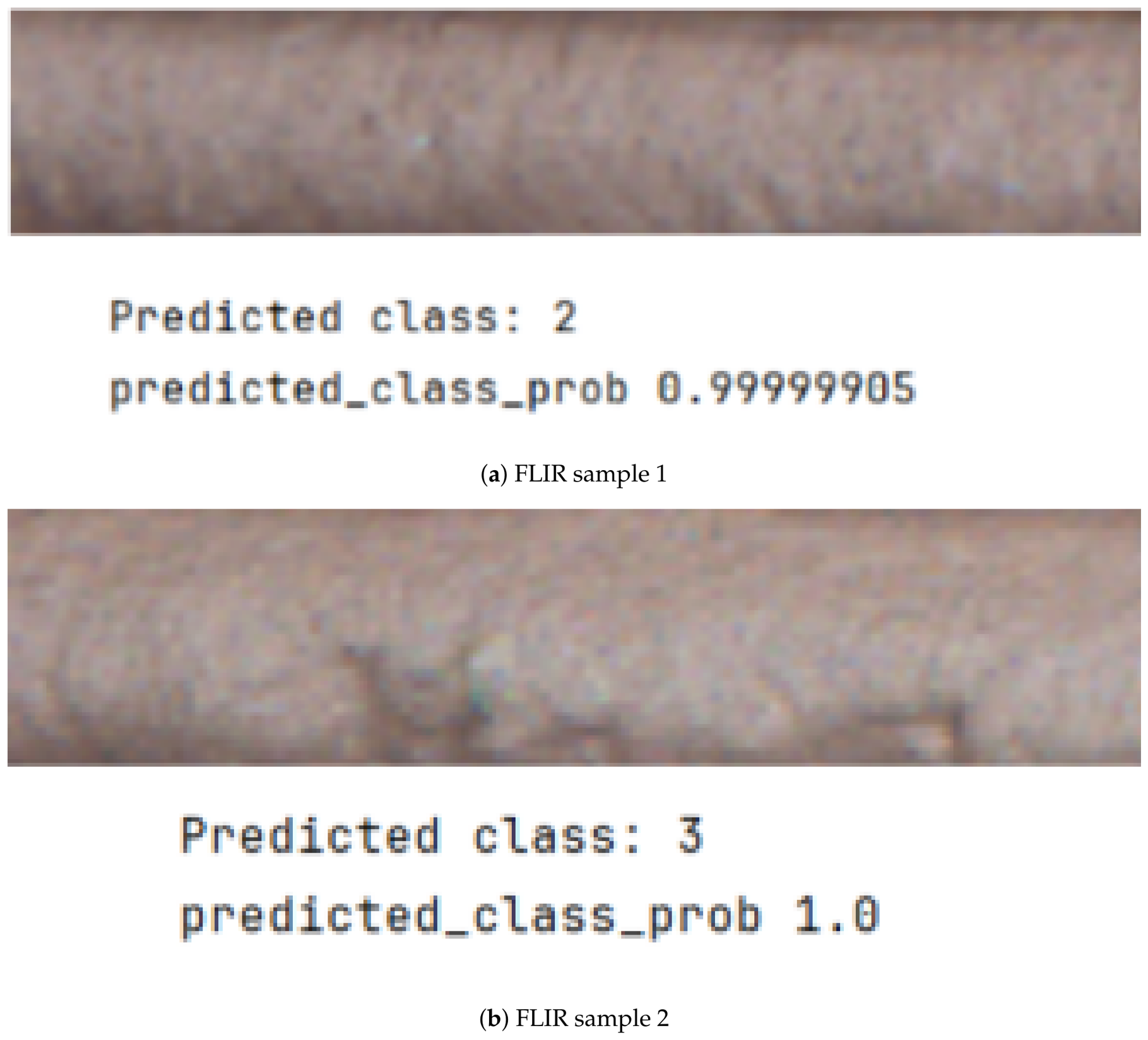
Figure 9.
Training and Validation Loss.
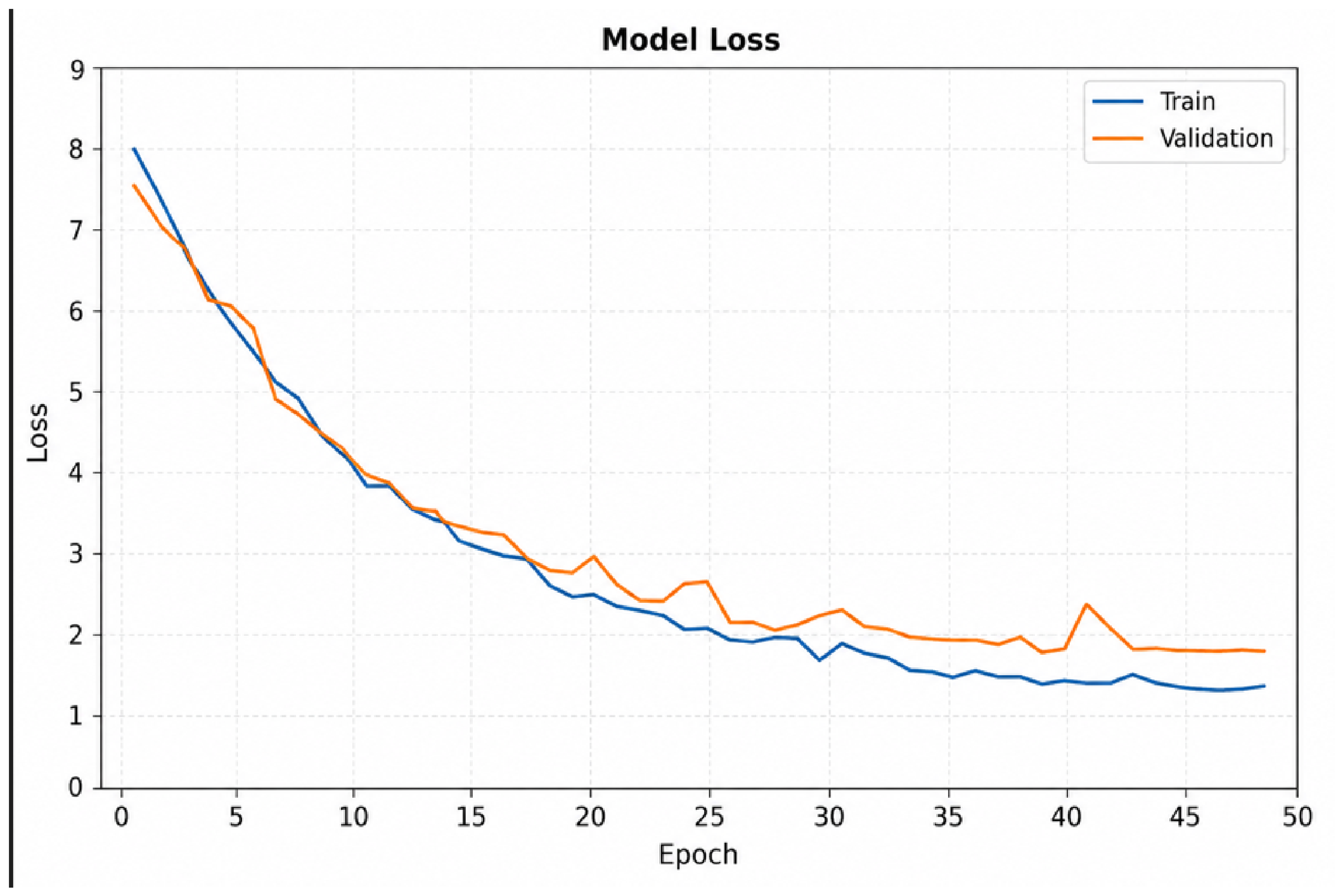
Figure 10.
F1 Score Across the Four Classes.
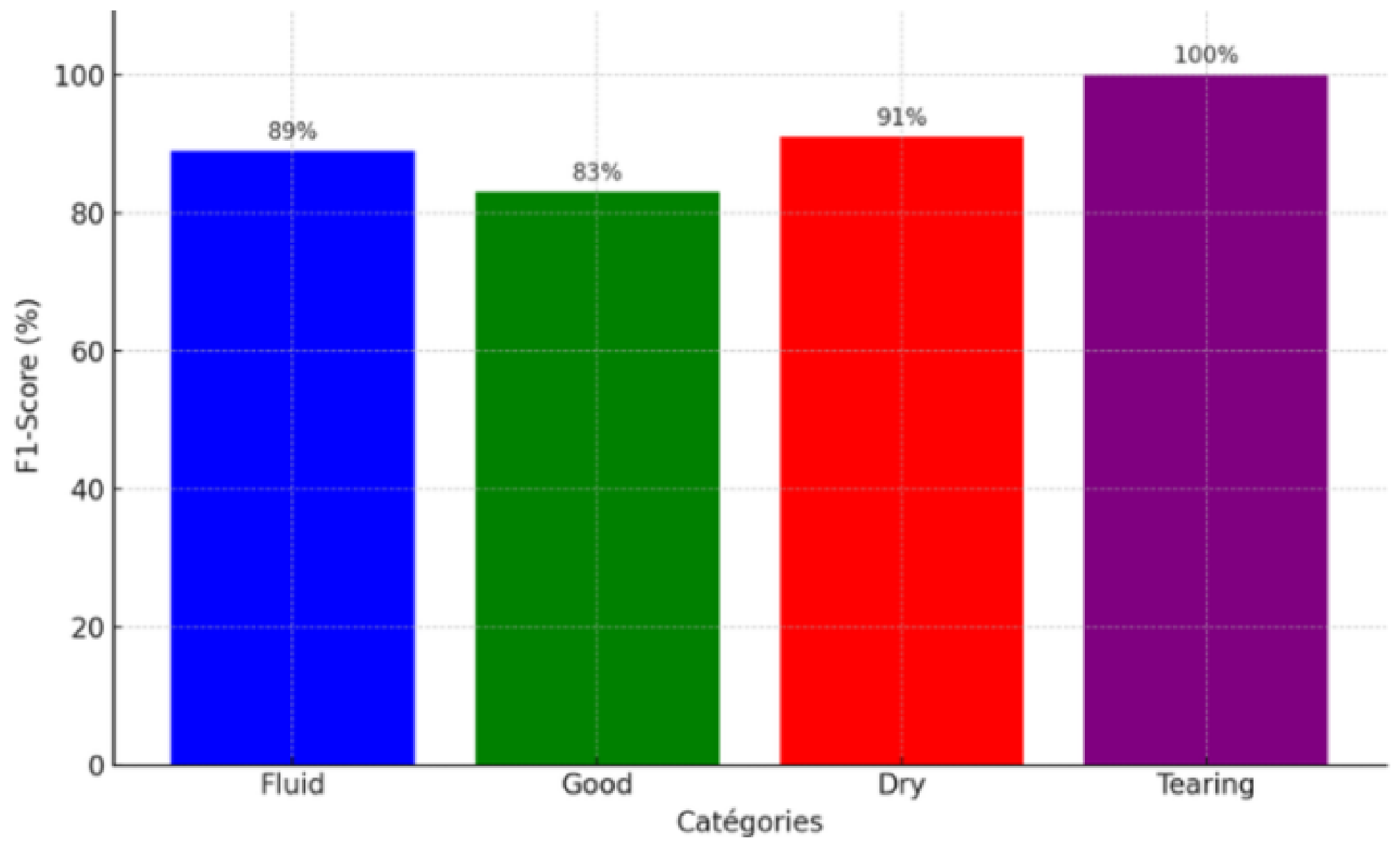

Table 1.
Optical and Operational Configuration of the Multi-Camera Vision System.
| Parameter | Camera A | Camera B | Camera C |
|---|---|---|---|
| Perspective | Front view | Nozzle-mounted view | Top view |
| Kinematics | Fixed (Stationary) | Mobile (Attached to nozzle at defined angle) | Fixed (Stationary) |
| Core Objective | Capture entire 15 cm wide object | Real-time deposition monitoring | Top-down surface analysis |
| Focal Length | mm | mm | or 25 mm |
| Target Defects | Interlayer size, macro-fissures | Porosities (air bubbles), micro-fissures | Porosities |
| Target Resolution | 2 mm (layer) / 150 m (fissures) | 150 m (fissures) / 100–150 m (porosities) | 100–150 m |
| Spatial Res. | 73.2 m/pixel | 19.531 m/pixel | – |
Table 2.
Summary of Dataset Partitioning and Data Augmentation Protocol.
| Pipeline Component | Technical Description and Parameters |
|---|---|
| Original Core Subset | 132 labeled RGB images with corresponding manual binary segmentation masks (3DCP concrete and clay-soil). |
| Preprocessing | The patch extraction represents pixels binary mask hreshold intensity normalization through binary value 0 or 255). |
| Data Partitioning | Training and validation split satisfying 80% 20% ratio utilizing random shuffling. |
| Spatial Augmentation | Simulation of alternative print layer directional orientations, adjusting horizontal and vertical axis flipping. |
| Geometric Shifts | To better induce structural and alignment variability. Discrete orthogonal rotations are applied across various angles (90°, 180°, 270°) |
| Photometric Shifts | Selective darkening and brightening coefficients to mimic shadows and brightness adjustments. |
| Noise Injection | To model industrial multi-sensor hardware artifacts, we simulate Gaussian blur and salt-and-pepper noise overlays. |
| Final Dataset Volume | Scalability to (660 operational images) by Multi-modal expansion yielding a matrix. |
Table 3.
U-VGG19 Segmentation Model Configuration
| Component | Description |
|---|---|
| Architecture | U-VGG19 (U-Net architecture with VGG19 encoder pretrained on ImageNet). |
| Encoder | VGG19-based feature extractor using convolutions, ReLU activations, and max-pooling layers. |
| Decoder | Upsampling path with convolutional layers to progressively reconstruct the segmentation map. |
| Skip connections | Concatenation between encoder and decoder feature maps to preserve spatial details. |
| Input size | RGB images. |
| Output layer | convolution followed by sigmoid activation for pixel-wise binary segmentation. |
| Loss function | Combination of Binary Cross-Entropy (BCE) and Dice Loss. |
| Optimizer | Adam optimizer. |
Table 4.
Model Added Layers and Training Parameters Architecture
| Layer / Parameter | Configuration |
|---|---|
| GlobalAveragePooling2D | Reduces feature map dimensionality. |
| Dense (Hidden) | 1024 units with ReLU activation and L2 regularization. |
| Dropout | Rate = 0.5 to reduce overfitting. |
| Dense (Output) | 4 neurons with Softmax activation (Fluid, Good, Dry, Tearing). |
| Learning Rate | 0.0001 for stable convergence. |
| Optimizer | Adam optimizer. |
| Loss Function | Sparse categorical cross-entropy. |
| Batch Size | 4 (training), 1 (validation). |
| Learning Rate Policy | Reduction on plateau strategy. |
| Early Stopping | Patience of 20 epochs without improvement. |
| Objective | Classification of extrusion states in additive manufacturing. |
Table 5.
Comprehensive Fine-Tuning Strategies and Layer Freezing Configurations.
| Layer Group | Status & Code | Operational Rationale & Details |
|---|---|---|
| Lower Layers | Frozen layer.trainable = False | All layers except the last six are configured as non-trainable to conserve foundational representations and generic features (such as edges and basic textures). |
| Last 6 Layers | Trainable layer.trainable = True | The final six upper layers are defined as trainable, allowing the model to adjust and fine-tune specifically to the new texture classes. |
| Overall Objective: This approach enhances the model’s performance while successfully minimizing the risk of overfitting, particularly when the dataset is relatively limited. | ||
Table 6.
Post-Processing Objectives for Segmented Images.
| Phase / Step | Operational Objectives & Rationale |
|---|---|
| Post-Processing | Refines segmentation results, eliminates residual artifacts, and extracts relevant geometric information. |
| Quality Assurance | Ensures higher precision in image analysis and geometric defect detection. |
Table 7.
Comparative analysis of additive manufacturing monitoring and deep learning methods focusing on stability, gradient sensitivity, and robustness in industrial printing environments.
Table 7.
Comparative analysis of additive manufacturing monitoring and deep learning methods focusing on stability, gradient sensitivity, and robustness in industrial printing environments.
| Reference (Authors, Year) | Basic Contribution | Method | Limitations | Relevance |
|---|---|---|---|---|
| Rill-García et al. (2022) [12] | Inline monitoring of 3D concrete printing | Computer vision-based monitoring pipeline | Sensitive to illumination and domain shift | Robust feature stability in AM processes |
| Shevchik et al. (2018) [3] | Acoustic emission monitoring in AM | Spectral CNN on sensor signals | No spatial segmentation, indirect observation | Shows limits of non-visual stability monitoring |
| Okaro et al. (2019) [4] | Fault detection in laser powder-bed fusion | Semi-supervised machine learning | Sensitive to noise and class imbalance | Motivates robust gradient-based learning |
| Buswell et al. (2018) [2] | Roadmap of concrete extrusion AM | Experimental process analysis | No deep learning or stability modeling | Identifies gap in AI-based AM monitoring |
| Scholz-Reiter et al. (2012) [6] | Surface inspection of micro-parts | Classical vision-based inspection | Poor robustness under lighting variation | Justifies deep feature extraction robustness |
| Krizhevsky et al. (2012) [8] | CNN breakthrough for image classification | Deep convolutional neural networks | Not designed for segmentation or process stability | Backbone of deep learning feature extraction |
| Redmon et al. (2016) [15] | Real-time object detection (YOLO) | Single-stage CNN detection | Bounding-box level only, weak localization precision | Motivates pixel-level segmentation need |
| Weiss et al. (2016) [9] | Survey of transfer learning | Feature reuse from pretrained models | Domain gap in industrial imaging | Supports pretrained VGG feature usage |
| Goodfellow et al. (2016) [10] | Deep learning foundations | Optimization and representation learning | No AM-specific stability modeling | Theoretical basis for gradient stability analysis |
| Guo et al. (2022) [11] | Stability of nonlinear CNN systems | Mathematical neural dynamics modeling | No real industrial image validation | Links stability theory to neural networks behavior |
| Szeliski (2022) [13] | Computer vision fundamentals | Geometric and photometric modeling | Limited industrial AM focus | Supports image-based AM analysis framework |
Table 8.
Ablation Study on Data Augmentation: Quantitative Segmentation Performance Evaluation.
| Method | Dice Score (%) | Precision (%) | Recall (%) |
|---|---|---|---|
| No Augmentation (NA) | 93.58 | 94.78 | 94.17 |
| With Augmentation (WA) | 98.86 | 98.92 | 99.02 |
Disclaimer/Publisher’s Note: The statements, opinions and data contained in all publications are solely those of the individual author(s) and contributor(s) and not of MDPI and/or the editor(s). MDPI and/or the editor(s) disclaim responsibility for any injury to people or property resulting from any ideas, methods, instructions or products referred to in the content. |
© 2026 by the authors. Licensee MDPI, Basel, Switzerland. This article is an open access article distributed under the terms and conditions of the Creative Commons Attribution (CC BY) license (http://creativecommons.org/licenses/by/4.0/).
Copyright: This open access article is published under a Creative Commons CC BY 4.0 license, which permit the free download, distribution, and reuse, provided that the author and preprint are cited in any reuse.


