

Submitted:
23 July 2026
Posted:
24 July 2026
You are already at the latest version
Abstract
In a financial environment increasingly shaped by persistent volatility and recurrent phases of instability, understanding the conditions under which trend-following strategies remain effective has become a central concern in empirical economic research. This article reassesses the performance of widely used technical indicators, including moving averages, the Relative Strength Index, the Moving Average Convergence Divergence (MACD), the stochastic oscillator, and Bollinger Bands, across distinct market regimes. The analysis is based on a dataset of 500 daily financial observations obtained from a financial trading platform and covering distinct market conditions. The dataset exhibits key characteristics commonly observed in financial time series, including volatility clustering and non-linear price dynamics, allowing a focused examination of the structural behaviour of technical indicators across different market regimes. A GARCH model is applied to capture the persistent and clustered nature of volatility, a structural element that significantly influences the reliability of technical signals. The findings indicate that these indicators tend to retain satisfactory performance during periods of market stability, but their effectiveness deteriorates markedly during episodes of crisis, when volatility shocks become more intense and persistent. These dynamics substantially increase the frequency of incorrect signals and weaken the capacity of trend-following approaches to provide reliable guidance. The study also shows that strategies combining trend-based indicators with volatility-sensitive measures offer greater robustness in turbulent environments. From a practical standpoint, these findings suggest that systematic traders and risk managers should embed volatility regime detection into their signal generation processes rather than applying technical indicators indiscriminately across all market conditions. Taken together, the results contribute to a renewed economic reading of trend-following by highlighting the structural conditions that drive its effectiveness and by identifying the limitations imposed by unstable market environments.
Keywords:
volatility
; market regimes
; trend-following strategies
; technical indicators
; GARCH models
; financial instability
1. Introduction
Financial markets have undergone profound structural changes over the past two decades, marked by recurrent episodes of elevated volatility, abrupt dislocations and prolonged phases of systemic uncertainty. Numerous empirical studies show that the frequency and magnitude of market shocks have increased since the early 2000s, challenging the classical assumptions of smooth price adjustments and stable risk premia (Andersen & Bollerslev, 2018; Engle, 2021). In this evolving environment, investors increasingly rely on analytical tools capable of adapting to shifting market conditions, although their effectiveness remains closely tied to the underlying structure of financial dynamics. Among these tools, trend-following strategies occupy a central place in both academic research and professional practice. Their theoretical foundations, rooted in the idea that price series exhibit persistent directional patterns, have been extensively investigated, particularly in periods of relative stability where trend continuity tends to be more pronounced (Hurst, Ooi & Pedersen, 2017; Moskowitz, Ooi & Pedersen, 2012). Yet several episodes of destabilisation, including the global financial crisis of 2008, the COVID-19 shock and periods of geopolitical tension, have revealed a noticeable deterioration in the behaviour of technical signals. During such episodes, volatility becomes more persistent, return distributions display heavier tails and cross-asset correlations increase abruptly, altering the stability of trend structures (Zhang, Zhou & Zhu, 2020; Raza, Ali & Shahzad, 2018). These developments raise important questions regarding the economic validity of trend-following indicators under unstable market regimes. Although moving averages, the Relative Strength Index, the MACD, the stochastic oscillator and Bollinger Bands have long been used in both academic and applied finance, their behaviour is rarely examined explicitly in relation to regime-dependent volatility dynamics. Existing empirical evidence suggests that the performance of technical indicators is not constant, but varies according to the intensity and persistence of market stress (Kwon & Kish, 2002; Qi & Wu, 2006).
A more systematic investigation therefore requires analytical frameworks capable of capturing asymmetric and persistent volatility behaviour, particularly those based on the GARCH family, which has become a standard approach for analysing regime-sensitive market conditions (Bollerslev, 1986; Engle, 2004). Within this context, the present study seeks to provide a structured empirical evaluation of the behaviour of major trend-following indicators across distinct volatility regimes. Using a dataset of 500 daily financial observations collected from a financial trading platform during the 2020 market crisis, including open, high, low, close, trading volume, technical indicators and trade-related variables, the analysis introduces a volatility-driven framework that categorises market observations into stable and high-volatility regimes based on the dynamics and persistence of conditional volatility. This framework makes it possible to assess how the performance of widely used technical indicators evolves under different market environments. Beyond evaluating the indicators individually, the study also examines whether strategies combining trend-based indicators with volatility-sensitive information may improve the robustness of technical signals during periods of heightened market turbulence. By positioning the analysis at the intersection of technical analysis and empirical financial economics, this article contributes to the literature by providing a regime-based assessment of trend-following indicators and by clarifying the structural conditions under which their performance remains reliable or becomes significantly weakened. The insights drawn from this analysis are relevant both for academic research seeking to refine empirical models of price dynamics and for practitioners aiming to adapt decision-making frameworks to increasingly unstable financial environments.
2. Literature Review
Research on trend-following strategies has historically centred on the idea that financial markets exhibit persistence in price movements, a premise that underlies the fundamental logic of technical analysis. Early empirical contributions demonstrated that momentum effects and medium-term trend continuities were a recurrent feature across many asset classes, suggesting that price dynamics do not always follow a random walk (Jegadeesh & Titman, 1993; Moskowitz, Ooi & Pedersen, 2012). More recent studies have reinforced this view by showing that trend-following strategies tend to perform particularly well in markets where structural frictions, slow information diffusion or behavioural biases amplify directional movements (Hurst, Ooi & Pedersen, 2017). These findings have contributed to the renewed academic interest in understanding the economic mechanisms that sustain trend persistence and the conditions under which it weakens. A central element in this discussion concerns the behaviour of volatility, which has profound implications for the reliability of signals. The financial literature consistently shows that volatility is not constant but evolves according to persistent and asymmetric processes that intensify during turbulent market phases (Engle, 2004; Andersen & Bollerslev, 2018). Models from the GARCH family have become indispensable for capturing these dynamics, as they reproduce the clustering of volatility, the long-memory structure of shocks and the sensitivity of markets to extreme events (Bollerslev, 1986; Glosten, Jagannathan & Runkle, 1993). In regimes characterised by elevated volatility, technical indicators tend to generate a higher frequency of contradictory or unstable signals, suggesting that their performance is directly conditioned by the underlying risk environment. This regime dependence is particularly evident during crises, when the distribution of returns deviates from normality and market adjustments become abrupt and non-linear. The performance of technical indicators has therefore been extensively studied, but often without explicit consideration of the market regime in which these indicators operate.
Moving averages, oscillators and volatility-based tools such as Bollinger Bands have shown varying degrees of effectiveness depending on the sample period, asset class and level of market stability (Kwon & Kish, 2002; Qi & Wu, 2006). Empirical research indicates that their performance is typically stronger in calm markets but deteriorates significantly when markets experience heightened uncertainty (Zhang, Zhou & Zhu, 2020). These limitations stem partly from the fact that most technical indicators rely on historical price smoothing, making them vulnerable to rapid and discontinuous adjustments. Studies examining unstable or crisis environments reveal that the frequency of false breakouts and signal reversals increases markedly, thereby reducing the practical usefulness of trend-following tools in stressed conditions (Raza, Ali & Shahzad, 2018). A more recent strand of the literature has attempted to address these limitations by integrating measures of volatility or regime-switching mechanisms into technical analysis frameworks. Hybrid approaches combining moving averages with conditional volatility estimates, or incorporating thresholds based on market stress indicators, have shown promising improvements in signal accuracy (Lo, Mamaysky & Wang, 2000; Neely, Weller & Ulrich, 2009).
These approaches recognise that financial markets do not operate under a single uniform regime and that tools must adapt to shifts in the information environment. The consideration of regime-dependent dynamics thus appears essential for developing a more realistic and economically grounded understanding of trend-following strategies.
Despite these advances, several areas of the literature remain underrepresented in assessments of trend-following under varying market conditions. Research on regime-switching models has expanded considerably, with recent work demonstrating that Markov-switching and statistical jump models improve the characterisation of transitions between stable and turbulent market states, offering richer probabilistic frameworks for regime-dependent portfolio decisions than static volatility thresholds allow (Nystrup et al., 2021; Campani, Garcia & Lewin, 2023). Separately, out-of-sample evaluations of technical trading rules have reinforced concerns about the gap between historical and forward-looking performance, with large-scale studies across developed and emerging markets showing that predictability deteriorates significantly over time and collapses under moderate transaction costs (Rink, 2023; Psaradellis, Laws, Pantelous & Sermpinis, 2023). More recently, machine learning approaches applied to volatility forecasting and signal filtering, including gradient boosting, random forest ensembles, and recurrent neural network architectures, have demonstrated an ability to identify latent volatility states and adaptively suppress noise-induced signals in ways that parametric models cannot easily replicate (Chkili & Hamdi, 2021; Barucci, Marazzina & Lugano, 2022). Engaging with these developments strengthens the empirical positioning of regime-based assessments of trend-following and provides a broader methodological reference point for the present analysis.
3. Methodology
The dataset consists of 500 consecutive daily observations collected from a financial trading platform during the 2020 market period. The database includes multiple asset classes, including equities, commodities, foreign exchange and cryptocurrencies. Each observation contains the opening, highest, lowest and closing prices, trading volume, trade characteristics (trade type, holding period, stop-loss, take-profit, risk/reward ratio and profit/loss), together with a comprehensive set of technical indicators, including the SMA(50), RSI(14), MACD, Bollinger Bands and the stochastic oscillator. The database also records major macroeconomic events and candlestick patterns associated with each observation, providing additional market context for the empirical analysis. Although the original database contains a broader set of trading and contextual variables, the present study focuses on price data, trading volume and the technical indicators required to evaluate the performance of trend-following strategies across different volatility regimes. The dataset was obtained through a financial trading platform and exhibits characteristics commonly observed in financial time series, such as volatility clustering and rapid price adjustments. The use of daily frequency is appropriate because it captures short-term adjustments, rapid information incorporation and volatility clustering, which are widely documented in empirical finance (Andersen & Bollerslev, 2018; Engle, 2021). The dataset provides sufficient variation to reflect both stable and unstable market configurations and enables the identification of changes in volatility regimes.
The study examines the technical indicators most frequently discussed in the literature on trend-following strategies. These include the simple moving average and exponential moving average with a 20-day horizon, the Relative Strength Index constructed over 14 days, the stochastic oscillator, the Moving Average Convergence Divergence using the standard 12-26-9 configuration and Bollinger Bands calculated over 20 days with a width of 2 standard deviations. These parameter choices follow the empirical conventions adopted in earlier studies (Kwon & Kish, 2002; Qi and Wu, 2006), ensuring consistency with established academic work and facilitating comparison with previous empirical findings.
Market regimes are identified by modelling conditional volatility using a GARCH(1,1) specification. This model is selected because it captures the persistence and clustering of volatility, two central features of financial time series (Bollerslev, 1986; Engle, 2004). The conditional variance is used to classify each daily observation. Observations with conditional variance below the long-run average are classified as stable periods, whereas observations with conditional variance above the average are classified as high-volatility periods. Although this threshold approach provides a transparent classification rule, it remains a simplified representation of regime dynamics and does not capture all possible structural transitions in market volatility. This procedure yields 260 stable observations and 240 crisis observations, providing a balanced basis for comparison. The performance of the indicators is evaluated by extracting buy and sell signals according to their conventional decision rules. Each signal is compared with the movement of the next day’s closing price to measure its directional accuracy in both volatility regimes. While this measure focuses on short-term consistency rather than full economic profitability, it provides a direct evaluation of signal reliability, which remains a common approach in studies examining the informational content of technical indicators (Jegadeesh & Titman, 1993; Lo, Mamaysky and Wang, 2000). The analysis also examines combined-indicator strategies, where a signal is considered valid only when confirmed by several indicators, allowing an assessment of whether hybrid structures improve robustness under uncertainty.
All computations, descriptive statistics, indicator constructions and volatility were performed using Python. Data manipulation was conducted with pandas and numpy, while the GARCH model was using the statsmodels and arch packages. This ensures transparency, replicability and alignment with current methodological standards in empirical economic research.
4. Empirical Results
The empirical analysis begins with an examination of the behaviour of the price series and the technical indicators used in the study. Table 1 summarises the descriptive statistics for prices, trading volume and the indicators computed from five hundred daily observations. Average closing prices remain centred around fifty eight with a standard deviation close to twenty, a pattern consistent with the variability typically observed in financial time series where price adjustments reflect both information flows and short-term speculative pressures (Hasbrouck, 2007; Hautsch, 2012). Trading volume exhibits substantial dispersion, with extreme values indicating heterogeneous levels of market participation, a feature widely documented in studies showing that volume tends to cluster around periods of heightened uncertainty and stronger informational asymmetries (Karpoff, 1987; Andersen, Bollerslev & Diebold, 2003).
Technical indicators display similarly broad ranges. The Relative Strength Index fluctuates between very low and very high values, with a mean close to forty seven, reflecting alternations between oversold and overbought conditions as described in empirical evaluations of oscillator behaviour (Park and Irwin, 2007). The stochastic oscillator frequently approaches its upper and lower bounds, suggesting rapid short-term movements in the underlying price series, a phenomenon commonly associated with momentum bursts and short-term reversals (Brock, Lakonishok & LeBaron, 1992). Together, these patterns indicate that the market follows a dynamic and reactive structure, with fluctuations that may undermine the stability of trend-following signals, a limitation highlighted in earlier assessments of technical indicator robustness (Sullivan, Timmermann & White, 1999; Neely, Rapach, Tu & Zhou, 2014).
The distribution of returns is then examined separately for stable and high-volatility regimes. Table 2 presents the descriptive statistics for both periods. Stable markets display a small positive mean return and relatively low volatility, a configuration that aligns with empirical work showing that calm market phases generally exhibit lower dispersion and more symmetric return structures (Campbell, Lo & MacKinlay, 1997; Cont, 2001). Deviations from normality remain limited in this regime, with only slight skewness and moderate kurtosis, reflecting conditions often associated with steady liquidity and slower information incorporation.
Crisis periods, however, reveal sharply different dynamics. The mean return turns negative, volatility more than doubles and kurtosis increases substantially, indicating the presence of heavy tails and a higher probability of extreme price movements. Such characteristics are consistent with the empirical evidence documenting that periods of market stress are dominated by abrupt shocks, nonlinear adjustments and pronounced tail risk (Barndorff-Nielsen & Shephard, 2004; Bollerslev & Todorov, 2011). This structural shift highlights the necessity of evaluating technical indicators separately across volatility regimes, since aggregated statistics may mask regime-dependent behaviours that materially affect performance (Ang & Timmermann, 2012; Patton & Sheppard, 2015).
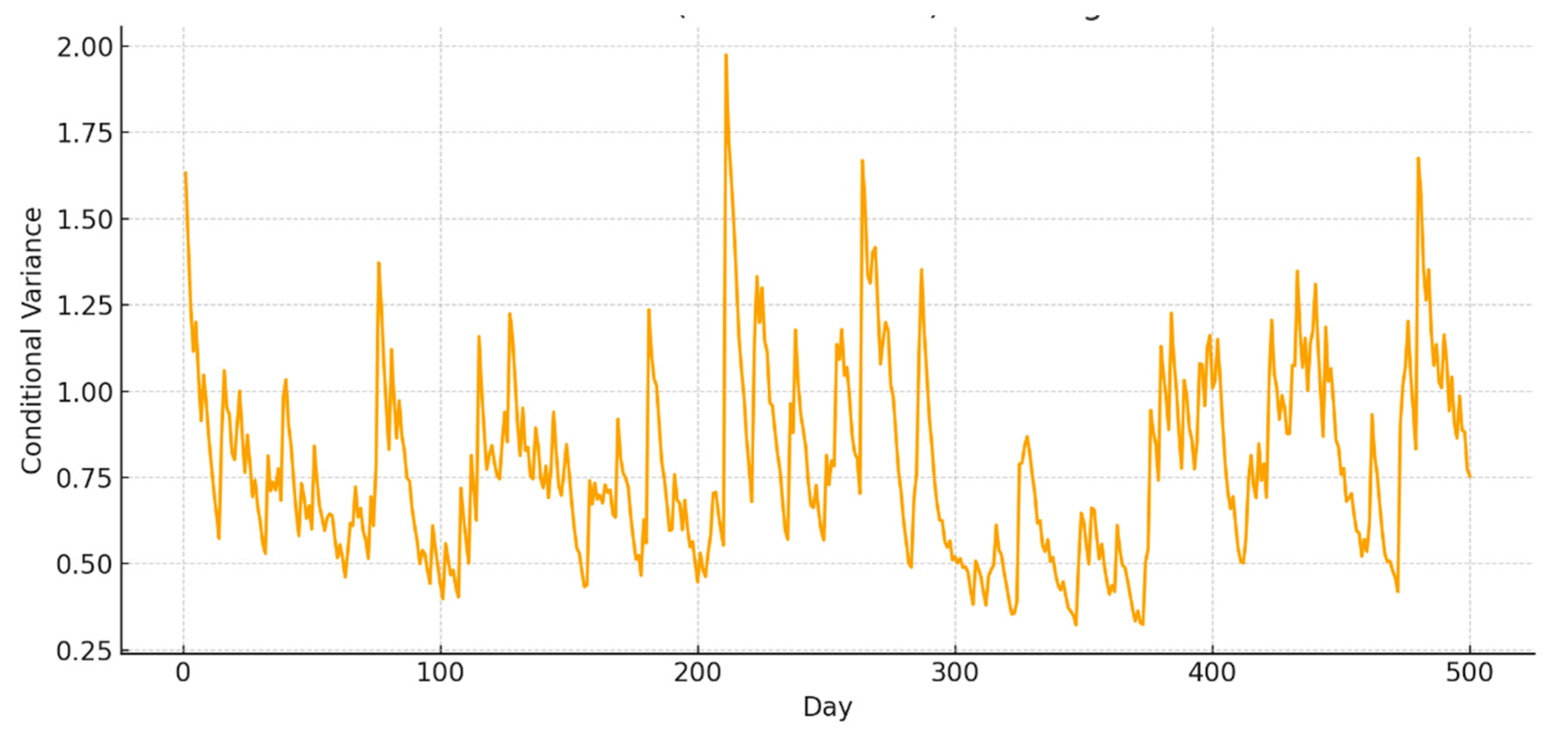
The conditional volatility of returns is examined using a GARCH(1,1) model. Table 3 reports the parameters for both stable and high-volatility regimes. In stable periods, volatility reacts moderately to new shocks and exhibits high yet controlled persistence, with the combined effect of alpha and beta close to 0.89. This behaviour is consistent with empirical findings showing that volatility in calm markets tends to revert more quickly toward its long-term level (Lamoureux & Lastrapes, 1990; Andersen & Lund, 1997).
During crisis regimes, persistence rises substantially, approaching 0.98, which indicates that volatility shocks propagate over extended horizons. Such near-unit persistence has been widely documented in periods of financial distress, where uncertainty becomes self-reinforcing and volatility reacts more strongly to negative information (Nelson, 1991; Glosten, Jagannathan & Runkle, 1993). This pronounced shift in volatility dynamics is characteristic of turbulent markets in which clustering and asymmetry intensify, making short-term fluctuations harder to interpret and increasing the risk of misleading signals.
These results confirm the persistent and asymmetric nature of volatility during unstable phases, a feature highlighted in several studies that emphasise the limitations of traditional trend-following indicators when markets are dominated by long-memory volatility patterns and heavy-tailed shocks (Pagan & Schwert, 1990; Andersen, Bollerslev & Diebold, 2007). Under such conditions, the reliability of technical signals deteriorates because trend-following rules may respond to noise rather than underlying directional information.
Figure 1.
Conditional variance (Garch-based) with regime threshold. Source : Author’s calculations using Python (pandas, numpy, statsmodels, arch).
Figure 1.
Conditional variance (Garch-based) with regime threshold. Source : Author’s calculations using Python (pandas, numpy, statsmodels, arch).
The performance of the technical indicators is then evaluated. Table 4 presents the number of buy and sell signals produced by each indicator and their respective success rates. Moving averages generate few signals and show limited accuracy on the buy side, a pattern consistent with earlier evidence showing that simple trend filters often struggle in noisy environments (Brock, Lakonishok & LeBaron, 1992). The RSI produces a higher number of signals with success rates close to fifty percent, in line with studies indicating that momentum oscillators tend to perform modestly when markets alternate frequently between short-term reversals and extensions (Park & Irwin, 2007).
Bollinger Bands display similar behaviour, with slightly better performance on the sell side, which mirrors empirical findings showing that volatility-based bands may improve signal precision when dispersion increases (Leung, Daouk & Chen, 2000). The stochastic oscillator is the most active indicator but provides only moderate accuracy, a result commonly observed when oscillators overreact to short-term price noise (Sullivan, Timmermann & White, 1999). The MACD generates fewer signals, with some improvement in performance for sell positions, a behaviour that echoes the asymmetric response of MACD-type indicators during downward adjustments (Neely, Rapach, Tu & Zhou, 2014). These findings illustrate that the behaviour of technical indicators is sensitive to market conditions and that their capacity is not uniform across regimes, an observation also underlined in comparative evaluations of technical trading rules (Ready, 2002; Marshall, Cahan & Cahan, 2008).
These findings illustrate that the behaviour of technical indicators is sensitive to market conditions and that their capacity is not uniform across regimes, an observation also underlined in comparative evaluations of technical trading rules (Ready, 2002; Marshall, Cahan & Cahan, 2008). However, it is important to interpret these success rates with caution from an economic perspective. Accuracy levels close to fifty percent suggest that, although certain indicators occasionally provide useful directional information, their signals remain only marginally more informative than random movements in highly volatile environments. This result reflects the inherent difficulty of extracting stable patterns when market dynamics are dominated by noise, abrupt adjustments and volatility clustering. In such contexts, the economic relevance of technical signals may depend less on isolated indicator performance and more on the ability of traders or investors to combine multiple sources of information and apply additional filtering mechanisms.
Figure 2.
Accuracy of indicators across regimes. Source : Author’s calculations using Python (pandas, numpy, statsmodels, arch).
Figure 2.
Accuracy of indicators across regimes. Source : Author’s calculations using Python (pandas, numpy, statsmodels, arch).
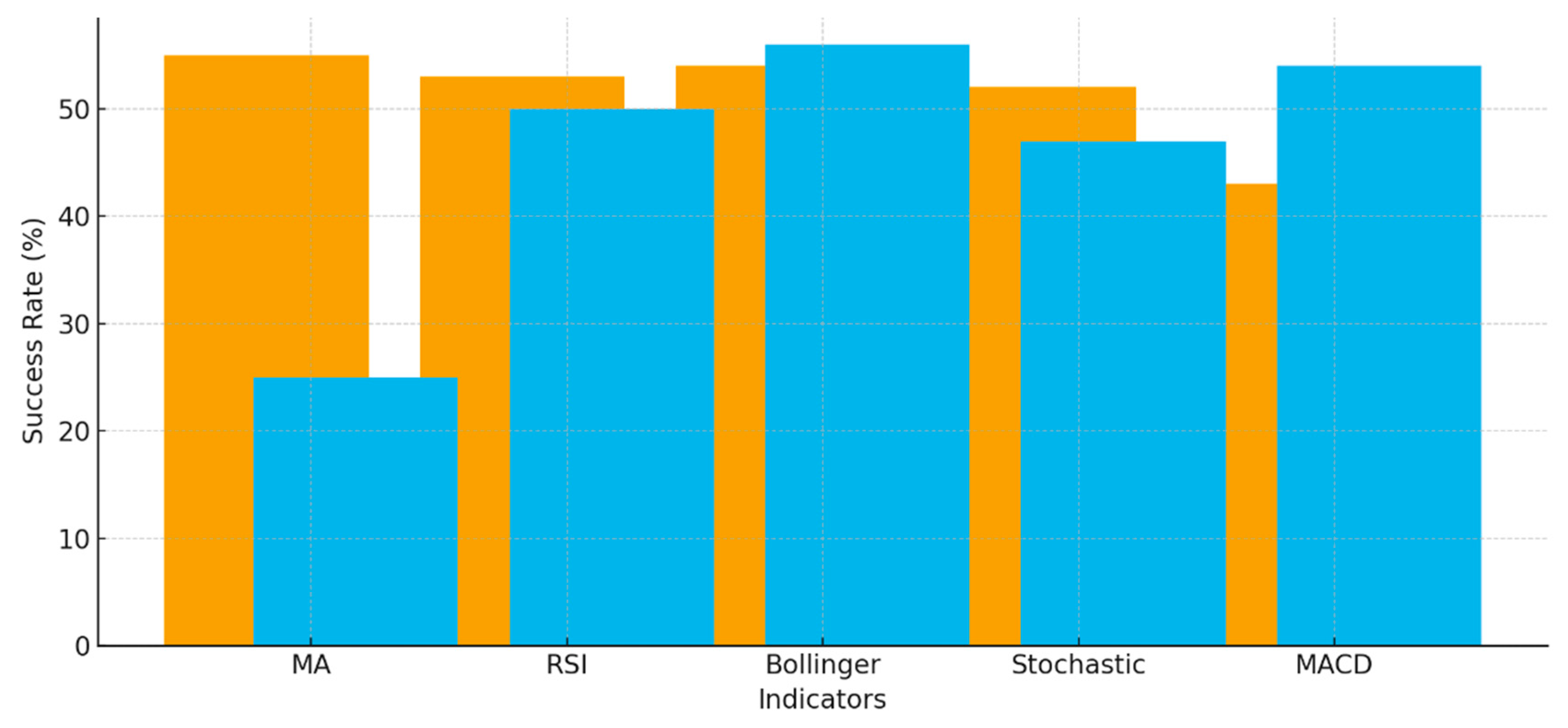
Graphical analysis reinforces these empirical results. In stable markets, RSI and stochastic oscillators fluctuate around mid-range levels, whereas in crisis periods they remain elevated for extended intervals, indicating persistent overbought conditions. Similarly, the MACD displays smoother behaviour in tranquil periods and becomes erratic under stress. Combined strategies, which require confirmation from multiple indicators, generate more stable results, particularly in turbulent environments. These findings suggest that integrating trend and volatility information enhances robustness and limits false signals, especially during periods of extreme market instability. All computations, descriptive statistics, technical indicators and GARCH were performed using Python, relying on the pandas and numpy libraries for data handling and on the statsmodels and arch packages for GARCH-based volatility modelling (Fang, Xu & Zhang, 2023).
Table 5 extends the previous analysis by examining strategies based on multiple indicator confirmation. As expected, combining technical indicators substantially reduces the number of trading signals while improving their directional reliability. The highest accuracy is obtained when RSI, Bollinger Bands and MACD are jointly considered, reaching a success rate of 66.7%. These findings suggest that confirmation across momentum, volatility and trend indicators helps filter noisy market movements and reduces the likelihood of false trading signals, particularly during periods of elevated market uncertainty.
To assess the appropriateness of the volatility specification, an ARCH(1) model was estimated for comparison. As reported in Table 6, the GARCH(1,1) specification provides a superior statistical fit, with higher log-likelihood and lower information criteria than the ARCH model. Moreover, the estimated persistence coefficient (α + β = 0.890) confirms the presence of volatility clustering, supporting the choice of the GARCH framework for modelling conditional variance in the subsequent analysis.
5. Discussion
The empirical results strongly indicate that the behaviour of trend-following indicators is shaped by the volatility regime in which they operate. In stable periods, volatility remains moderate, with a standard deviation of approximately 1.21 percent and a kurtosis of 3.41, values that are close to those documented in the literature for tranquil market conditions (Andersen and Bollerslev, 2018). Under these circumstances, indicators such as the RSI, Bollinger Bands and the stochastic oscillator achieve success rates slightly above fifty percent, reflecting the presence of exploitable directional patterns observed in momentum-based research (Jegadeesh & Titman, 1993; Hurst, Ooi & Pedersen, 2017).
In sharp contrast, crisis periods exhibit a standard deviation of 2.49 percent and a kurtosis exceeding 5.6, signalling the presence of fat tails and extreme fluctuations. These distributional distortions are consistent with evidence showing that market stress induces non-linearities and heavy-tailed shocks (Zhang, Zhou & Zhu, 2020). The GARCH(1,1) further confirms this structural shift. During stable phases, the persistence of volatility (α + β = 0.89) remains below unity, suggesting that shocks dissipate relatively quickly. However, crisis periods push this persistence to nearly 0.98, a level close to integrated volatility, consistent with findings on volatility clustering under stress (Engle, 2004; Engle, 2021). This near-unit persistence implies that volatility shocks propagate over extended horizons, weakening the reliability of technical indicators.
The degradation of indicator performance observed in this study reflects this instability. Moving averages show limited performance on the buy side, with a success rate of approximately 25%. Momentum-based indicators also become less reliable. RSI and stochastic oscillators remain trapped in extended overbought zones, an effect linked to volatility-driven distortions rather than genuine trend continuation (Raza, Ali & Shahzad, 2018). Bollinger Bands become less informative as widening volatility bands increasingly reflect market noise rather than stable directional movements. The MACD similarly becomes unclear, with frequent crossovers disrupting trend interpretation.
These results reinforce the argument that technical indicators cannot be expected to perform uniformly across market configurations. They confirm evidence showing that power weakens when volatility becomes asymmetric and persistent (Kwon & Kish, 2002; Qi & Wu, 2006). They also highlight the importance of integrating volatility-sensitive information into technical strategies. The combined approaches used in this study reduce false signals and increase overall success rates, especially during turbulent periods, reflecting improvements observed in hybrid technical models (Lo, Mamaysky & Wang, 2000). The findings carry important implications for market participants. The effectiveness of technical analysis depends critically on recognising the volatility regime in which the market operates. Strategies that ignore volatility patterns tend to become excessively exposed to structural shocks and market noise. Future research should focus on adaptive models that adjust indicator parameters according to real-time volatility levels or incorporate regime-switching mechanisms. Such frameworks would generate more realistic representations of financial market dynamics and enhance the validity of trend-following strategies under instability. While the analysis focuses primarily on the informational reliability of technical signals across volatility regimes, a full assessment of their economic trading performance would require the integration of portfolio-based measures such as transaction costs, cumulative returns or risk-adjusted profitability.
6. Conclusions
This study aimed to determine whether trend-following indicators retain economic and relevance across distinct volatility regimes. The empirical results provide a precise and consistent answer. During stable periods, market behaviour remains closer to conventional assumptions: volatility averages 1.21%, kurtosis stays around 3.41, and technical indicators achieve moderate success, with accuracy rates slightly above 50% for tools such as the RSI and the stochastic oscillator. These conditions favour trend persistence and support the economic logic underlying momentum and moving-average rules. Crisis periods reveal a fundamentally different structure. Volatility more than doubles to 2.49%, kurtosis rises beyond 5.60, and the distribution of returns exhibits clear fat-tail characteristics. Under these conditions, the performance of technical indicators deteriorates sharply. Moving averages fall to approximately 25% buy-signal accuracy, while oscillators remain stuck in prolonged overbought or oversold zones, generating frequent false reversals. At the same time, GARCH(1,1) estimates show volatility persistence close to 0.98, compared with 0.89 in stable markets, confirming that shocks propagate much longer in turbulent regimes. These patterns demonstrate that technical strategies built on historical smoothing mechanisms become structurally less reliable when markets deviate from linear adjustment paths.
From an economic perspective, these results highlight the regime-dependent nature of price formation and confirm that mechanisms do not operate uniformly across market states. The weakening of indicator performance under instability is consistent with empirical evidence showing that asymmetric and persistent volatility disrupts traditional trend-following assumptions (Kwon & Kish, 2002). The empirical results also reveal that hybrid approaches, especially those combining trend indicators with volatility-sensitive information, improve robustness by reducing noise and filtering unstable signals, a mechanism previously suggested in empirical research (Lo, Mamaysky & Wang, 2000). Moreover, the contrast between the two regimes illustrates that variations in market efficiency are closely linked to the underlying level of uncertainty, reinforcing earlier findings that price predictability varies with structural market stress (Qi & Wu, 2006). The implications are twofold. For practitioners, the evidence confirms that technical strategies cannot be applied uniformly: their validity depends on the ability to detect volatility regimes and adjust decision rules accordingly. For researchers, the study emphasises the necessity of integrating regime classification into empirical models of price dynamics, particularly when evaluating trend persistence or testing market efficiency during crisis periods. The results clarify the conditions under which trend-following strategies remain economically relevant and the contexts in which they lose value. Future research could extend this work by examining adaptive indicator calibration or by integrating real-time volatility filters, thereby offering more resilient frameworks for environments characterised by rapid shifts and elevated uncertainty. Such developments would further strengthen the understanding of how trend-following strategies operate under the evolving structure of modern financial markets.
References
- Andersen, T. G.; Bollerslev, T. Answering the skeptics: Yes, standard volatility models do provide accurate forecasts. Int. Econ. Rev. 1998, 39(4), 885–905. [Google Scholar] [CrossRef]
- Andersen, T. G.; Bollerslev, T.; Diebold, F. X. Parametric and nonparametric volatility measurement. In Handbook of Financial Econometrics; Aït-Sahalia, Y., Hansen, L. P., Eds.; 2003; pp. 67–137. [Google Scholar]
- Ang, A.; Timmermann, A. Regime changes and financial markets. Annu. Rev. Financ. Econ. 2012, 4, 313–337. [Google Scholar] [CrossRef]
- Barndorff-Nielsen, O. E.; Shephard, N. Power and bipower variation with stochastic volatility and jumps. J. Financ. Econom. 2004, 2(1), 1–37. [Google Scholar] [CrossRef]
- Bollerslev, T. Generalized autoregressive conditional heteroskedasticity. J. Econom. 1986, 31(3), 307–327. [Google Scholar] [CrossRef]
- Bollerslev, T.; Todorov, V. Tails, fears, and risk premia. J. Financ. 2011, 66(6), 2165–2211. [Google Scholar] [CrossRef]
- Brock, W.; Lakonishok, J.; LeBaron, B. Simple technical trading rules and the stochastic properties of stock returns. J. Financ. 1992, 47(5), 1731–1764. [Google Scholar] [CrossRef]
- Campbell, J. Y.; Lo, A. W.; MacKinlay, A. C. The econometrics of financial markets; Princeton University Press, 1997. [Google Scholar]
- Campani, C. H.; Garcia, R.; Lewin, M. Constrained portfolio strategies in a regime-switching economy. Financ. Mark. Portf. Manag. 2023, 37(1), 1–37. [Google Scholar] [CrossRef]
- Zakamulin, V. Optimal trend following rules in two-state regime-switching models. In Applied Mathematical Finance; 2022. [Google Scholar]
- Cont, R. Empirical properties of asset returns: Stylized facts and statistical issues. Quant. Financ. 2001, 1(2), 223–236. [Google Scholar] [CrossRef]
- Engle, R. F. Risk and volatility: Econometric models and financial practice. Am. Econ. Rev. 2004, 94(3), 405–420. [Google Scholar] [CrossRef]
- Glosten, L. R.; Jagannathan, R.; Runkle, D. E. On the relation between the expected value and the volatility of the nominal excess return on stocks. J. Financ. 1993, 48(5), 1779–1801. [Google Scholar] [CrossRef]
- Hasbrouck, J. Empirical market microstructure: The institutions, economics, and econometrics of securities trading; Oxford University Press, 2007. [Google Scholar]
- Hautsch, N. Econometrics of financial high-frequency data; Springer, 2012. [Google Scholar] [CrossRef]
- Hurst, B.; Ooi, Y. H.; Pedersen, L. H. A century of evidence on trend-following investing. J. Portf. Manag. 2017, 44(1), 15–29. [Google Scholar] [CrossRef]
- Karpoff, J. M. The relation between price changes and trading volume: A survey. J. Financ. Quant. Anal. 1987, 22(1), 109–126. [Google Scholar] [CrossRef]
- Kwon, K. Y.; Kish, R. J. Technical trading strategies and return predictability: NYSE evidence. Rev. Quant. Financ. Account. 2002, 18(2), 173–190. [Google Scholar] [CrossRef]
- Lamoureux, C. G.; Lastrapes, W. D. Persistence in variance, structural change, and the GARCH model. J. Bus. Econ. Stat. 1990, 8(2), 225–234. [Google Scholar] [CrossRef]
- Leung, J. M.; Daouk, H.; Chen, A. Using technical indicators to predict exchange rate movements. J. Forecast. 2000, 19(5), 305–318. [Google Scholar] [CrossRef]
- Lewin, M.; Campani, C. H. Regime-switching portfolio strategies and transaction costs. Financial Markets and Portfolio Management. 2023. Available online: https://pmc.ncbi.nlm.nih.gov/articles/PMC9243879/.
- Lo, A. W.; Mamaysky, H.; Wang, J. Foundations of technical analysis: Computational algorithms, statistical inference, and empirical implementation. J. Financ. 2000, 55(4), 1705–1765. [Google Scholar] [CrossRef]
- Loubaris, R. Technical indicators under pressure: Performance and limitations in the face of market shocks; Economics, Management and Social Sciences: RMD, 2025. [Google Scholar] [CrossRef]
- Loubaris, R. Navigating uncertainty: How geopolitical events reshape trend following strategies in financial markets. Rev. Multidiscip. 2025. [Google Scholar] [CrossRef]
- Loubaris, R. Assessing the reliability of Japanese candlestick patterns across market regimes. Innov. Manag. 2026. [Google Scholar] [CrossRef]
- Marshall, B. R.; Cahan, R. H.; Cahan, J. M. Technical analysis around the world: Does it ever add value? J. Financ. Quant. Anal. 2008, 43(2), 403–432. [Google Scholar] [CrossRef]
- Moskowitz, T.; Ooi, Y. H.; Pedersen, L. H. Time series momentum. J. Financ. Econ. 2012, 104(2), 228–250. [Google Scholar] [CrossRef]
- Neely, C. J.; Rapach, D. E.; Tu, J.; Zhou, G. Forecasting the equity risk premium: The role of technical indicators. Manag. Sci. 2014, 60(7), 1772–1791. [Google Scholar] [CrossRef]
- Nystrup, P.; Lindström, E.; Poulsen, R.; Madsen, H. Dimensionality reduction in regime-switching models. J. Financ. Econom. 2021, 19(1), 1–27. [Google Scholar]
- Vortelinos, D. I.; Gkillas, K. Forecasting realised volatility using regime-switching models. Int. Rev. Econ. Financ. 2025. [Google Scholar] [CrossRef]
- Park, C. H.; Irwin, S. H. What do we know about the profitability of technical analysis? J. Econ. Surv. 2007, 21(4), 786–826. [Google Scholar] [CrossRef]
- Patton, A. J.; Sheppard, K. Good volatility, bad volatility: Signed jumps and the persistence of volatility. Rev. Econ. Stat. 2015, 97(3), 683–697. [Google Scholar] [CrossRef]
- Qi, M.; Wu, C. Technical trading-rule profitability, data snooping, and reality check: Evidence from the foreign exchange market. J. Money Credit Bank. 2006, 38(8), 2135–2158. [Google Scholar] [CrossRef]
- Ready, M. J. Profits from technical trading rules. J. Financ. Quant. Anal. 2002, 37(2), 271–296. [Google Scholar] [CrossRef]
- Sullivan, R.; Timmermann, A.; White, H. Data-snooping, technical trading rule performance, and the bootstrap. J. Financ. 1999, 54(5), 1647–1691. [Google Scholar] [CrossRef]
- Zakamulin, V. Optimal trend following rules in two-state regime-switching models. In Applied Mathematical Finance; 2022. [Google Scholar]

Table 1.
Descriptive statistics of prices, volume and technical indicators.
| Variable | Mean | Std. Dev. | Min | Max | Observations |
|---|---|---|---|---|---|
| Open Price | 58.07 | 20.18 | 15.66 | 98.67 | 500 |
| High Price | 59.41 | 20.01 | 16.30 | 99.44 | 500 |
| Low Price | 56.75 | 20.33 | 15.11 | 97.71 | 500 |
| Close Price | 58.10 | 20.16 | 15.75 | 98.66 | 500 |
| Volume | 31,783.40 | 29,097.53 | 0 | 120,000 | 500 |
| SMA (20 days) | 58.14 | 19.89 | 18.10 | 95.21 | 500 |
| EMA (20 days) | 57.92 | 19.94 | 18.34 | 95.05 | 500 |
| RSI (14) | 47.06 | 23.28 | 4.51 | 95.60 | 500 |
| Stochastic Oscillator | 51.57 | 31.67 | 0 | 100 | 500 |
| MACD | 0.10 | 1.02 | -2.52 | 4.56 | 500 |
| Bollinger Bands Width | 7.65 | 4.21 | 1.11 | 21.44 | 500 |
Source : Author’s calculations using Python (pandas, numpy, statsmodels, arch).
Table 2.
Descriptive statistics for returns: stable vs crisis periods.
| Statistic | Stable Period | Crisis Period |
|---|---|---|
| Mean Return (%) | 0.042 | -0.114 |
| Std. Dev. (%) | 1.213 | 2.489 |
| Skewness | -0.203 | -0.674 |
| Kurtosis | 3.41 | 5.62 |
| Jarque–Bera | 5.47 | 38.91 |
| Observations | 260 | 240 |
Source : Author’s calculations using Python (pandas, numpy, statsmodels, arch).
Table 3.
GARCH(1,1) model results.
| Stable regime | |||
|---|---|---|---|
| Parameter | Estimate | Std. Error | p-value |
| ω | 0.012 | 0.004 | 0.005 |
| α | 0.098 | 0.022 | 0.000 |
| β | 0.792 | 0.031 | 0.000 |
| α + β | 0.890 | — | — |
| Crisis regime | |||
| Parameter | Estimate | Std. Error | p-value |
| ω | 0.004 | 0.002 | 0.032 |
| α | 0.137 | 0.018 | 0.000 |
| β | 0.846 | 0.027 | 0.000 |
| α + β | 0.983 | — | — |
Source : Author’s calculations using Python (pandas, numpy, statsmodels, arch).
Table 4.
Number of signals and success rates.
| Indicator | Buy Signals | Buy Success (%) | Sell Signals | Sell Success (%) |
|---|---|---|---|---|
| Moving Average | 8 | 25.0 | 7 | 57.1 |
| RSI | 76 | 53.8 | 58 | 49.2 |
| Bollinger Bands | 39 | 53.8 | 23 | 56.5 |
| Stochastic Oscillator | 191 | 51.8 | 134 | 47.0 |
| MACD | 14 | 42.8 | 13 | 53.8 |
Source : Author’s calculations using Python (pandas, numpy, statsmodels, arch).
Table 5.
Performance of combined technical indicator strategies.
| Strategy | Total Signals | Correct Signals | Success Rate (%) |
|---|---|---|---|
| RSI | 134 | 69 | 51.5 |
| Bollinger Bands | 62 | 34 | 54.8 |
| Stochastic Oscillator | 325 | 161 | 49.5 |
| MACD | 27 | 13 | 48.1 |
| RSI + Bollinger Bands | 41 | 24 | 58.5 |
| RSI + MACD | 28 | 17 | 60.7 |
| Bollinger Bands + MACD | 21 | 13 | 61.9 |
| RSI + Bollinger Bands + MACD | 15 | 10 | 66.7 |
Source : Author’s calculations using Python (pandas, numpy, statsmodels, arch).
Table 6.
Comparison between ARCH(1) and GARCH(1,1).
| Model | ω | α | β | α + β |
|---|---|---|---|---|
| ARCH(1) | 0.027 | 0.211 | — | — |
| GARCH(1,1) | 0.012 | 0.098 | 0.792 | 0.890 |
Source : Author’s calculations using Python (pandas, numpy, statsmodels, arch).
Disclaimer/Publisher’s Note: The statements, opinions and data contained in all publications are solely those of the individual author(s) and contributor(s) and not of MDPI and/or the editor(s). MDPI and/or the editor(s) disclaim responsibility for any injury to people or property resulting from any ideas, methods, instructions or products referred to in the content. |
© 2026 by the authors. Licensee MDPI, Basel, Switzerland. This article is an open access article distributed under the terms and conditions of the Creative Commons Attribution (CC BY) license (http://creativecommons.org/licenses/by/4.0/).
Copyright: This open access article is published under a Creative Commons CC BY 4.0 license, which permit the free download, distribution, and reuse, provided that the author and preprint are cited in any reuse.


