

Submitted:
10 July 2026
Posted:
24 July 2026
You are already at the latest version
Abstract
The focus and objective of this study are to conduct a comprehensive evaluation of the impact of the trade war between the United States and China, examining the degree of integration and causal relationships, as well as its spillover effects on stock and international financial markets in Asia and the United States. The data used were obtained by selecting a sample of 11 stock market indices from both regions, with monthly data covering the period from 2017 to 2024. The methodological approach to data analysis involved applying the Vector Error Correction Model (VECM) test, combined with the Granger Causality test, Johansen Cointegration, and the Impulse Response Function (IRF), as well as forecasting using the Forecast Error Variance Decomposition (FEVD) approach. The results of this study provide evidence that the greatest spillover effects and impacts are found in the stock and financial markets of Singapore, Japan, the Philippines, China and the United States. This implies a strong relationship between the stock markets in these two regions. Using the IRF and FEVD methods, it has been demonstrated that external shocks result in significant changes, whilst also showing that market volatility is temporary and will return to equilibrium once economic and financial stability is restored in both Asia and the United States. Fundamentally, the novelty of this research lies in simultaneously testing 11 stock markets across Asia and the United States, demonstrating that the trade war between the United States and China has triggered a paradigm shift: it is not only bilateral relations that are affected by this conflict, but the trade war also has implications for other countries or regions, where market integration, spillover effects and dynamic inter-market interdependence are evident. Thus, the findings of this study demonstrate that the interconnectedness of capital markets, both regionally and globally, is very strong and simultaneously reduces the effectiveness of international diversification strategies in decision-making due to the trade war between these two countries.
Keywords:
trade war
; spillover
; integration
; causality
; decomposition
1. Introduction
The capital market is a place where people with money can invest their funds, and where those in need of money can raise capital (Kakran et al., 2024). Furthermore, the capital market also plays a role in raising funds and raising public awareness of investment. This indirectly influences labour-sector production efficiency and productivity, thereby further strengthening the economy (Faniband, 2026; Hoque et al., 2023). The capital market is regarded as an integral part of the economy because it facilitates the relationship between investors or those with funds and those in need of funds, such as companies seeking to expand their operations (Zhao & Park, 2024; Enebeli et al., 2026). With the existence of the capital market, business operators have more funding options, enabling businesses to grow more rapidly. Consequently, business revenue and general welfare can increase (Salachas et al., 2024; Tran et al., 2023).
Rising share prices signal positive developments in the capital market that can support overall market growth (Tran et al., 2023; Zhang et al., 2023). Generally speaking, globalisation has made it easier for portfolio investments to enter the stock market. This can affect the stability of the local financial sector due to the inflow of foreign capital. A rise in stock market value can facilitate capital flows, improve the balance of payments, and boost the exchange rate (Pan et al., 2023; Zeng et al., 2025). A rise in stock market value is equivalent to an increase in market capitalisation. Market capitalisation is a measure of a company’s total value, calculated by multiplying the number of shares in circulation by the market price per share. Investors frequently use this term to assess a company’s quality. By knowing the market capitalisation, investors can determine how much money would be required to purchase all of the company’s shares (Su et al., 2025; Lean et al., 2024). Consequently, market capitalisation can be likened to situations such as the trade war between the United States and China in 2018, the global pandemic in 2020, the Russia–Ukraine conflict in 2022, and the resurgence of the trade war between the United States and China in early 2025. These events generated negative sentiment towards the capital markets and led to a decline in market capitalisation (Chen & Sun, 2024; Hu & Borjigin, 2024; Triansyah & Karyono, 2026).
The trade war between the United States and China has been affecting the global economy since 2018. The United States and China, two of the world’s economic powers, were embroiled in a trade war that imposed tariffs with negative effects on the global economic order. With Trump’s return as leader of the United States and as part of his economic policy to protect domestic products by 2025, tariffs on Chinese goods, including technology products, electric vehicles, and solar panels, have risen (Chen et al., 2023; Peng et al., 2025).
On the other hand, China has not stood idly by, imposing stricter import tariffs on products from the United States, such as agricultural and energy products and restricting metal exports to the United States for the technology industry. Consequently, the trade war between these two economic superpowers has disrupted and destabilised the global macroeconomy and financial system. From an international finance perspective, the implications of the tariff policy changes by both countries in the form of a trade war have led to a decline in business and trade activity among other nations, with the two countries involved in the tariff conflict (Fishman, 2025; Xu et al., 2024; He et al., 2021).
Another particularly worrying consequence of this trade war is that businesses have been forced to reassess their export and import costs. This has led to a loss of confidence among global and Asian businesses when making investment decisions, as the trade war has created uncertainty and hampered economic growth (You et al., 2024; Li et al., 2024).
Consequently, investors are becoming more cautious in their investment decisions, thereby hampering economic growth (You et al., 2024; Li et al., 2024). The tariffs imposed by the United States and China have raised import costs. Consequently, consumers and businesses in Asian countries, particularly those reliant on imports from the United States and China, are feeling the strain. In terms of investment shifts, Asian companies may move their funds from the United States or China to more stable countries. This may also present opportunities for Asian countries, as investment destinations, to boost economic growth and inflows of foreign direct investment (Aba, 2021; Baldwin, 2025).
Based on the preceding discussion and the issues at hand, this study aims to analyse financial integration as evidence of capital flows and causal relationships in the Asian and US stock markets resulting from the trade war between the two countries. This research is important for understanding how macroeconomic factors influence stock market indices, particularly in emerging Asian economies. Therefore, this study will analyse both unidirectional and bidirectional relationships among variables to determine which variables have greater influence in the short- and long-term. The variables examined are the stock market indices of Indonesia (JKSE), China (SSE), South Korea (KOSPI), the Philippines (PSEi), Malaysia (KLCI), Singapore (STI), Vietnam (VN-INDEX), Japan (NIKKEI 225), Thailand (SET INDEX), Taiwan (TSE 50), and the United States (DJIA).
2. Literature Review and Theoretical Background
To achieve the research objectives, data analysis was conducted using the Vector Autoregressive (VAR) and Vector Error Correction Model (VECM) methods. The data used in this study comprises monthly stock market indices for the period from January 2017 to December 2024, as well as projections for 2025 and 2026. These data sources are secondary and were obtained from official websites with international credibility.
2.1. Economic Integration, Stock Indices and Stationarity
A stationarity test, or unit root test, is a method used to determine whether a time series is stationary. Stationarity is an important requirement in econometric models that use time-series data. Stationary data has a mean, variance and autocorrelation that remain constant over time. With stationary data, time-series models are considered more stable and can provide more accurate results.
The purpose of this stationarity test is to determine whether the time series data are stationary. If the data are non-stationary, the likelihood of spurious regression increases. Typically, time series data used in research are non-stationary at the initial stage. To address this, the data needs to be differentiated once or twice to make it stationary. One method is to use the unit root test, namely the Augmented Dickey-Fuller (ADF) test (Tabash et al., 2024; Yilmazkuday, 2025).
When assessing the results of a stationarity test, in addition to the ADF statistic and the MacKinnon critical value, the probability value (p-value) may also be used. If the probability value is less than the significance level (α = 1%, 5% or 10%), the data are considered to have no unit root and to be non-stationary. Conversely, if the p-value exceeds α, the data exhibit a unit root and are non-stationary. Before performing regression on time-series data, the first step is to conduct a stationarity test. A stochastic process typically generates time-series data. Such data is said to be stationary if it satisfies three conditions: its mean and variance remain constant over time, and the covariance between two data points depends solely on the lag between them.
Stationary data have the same mean, variance and covariance at every point in time. If these three conditions are not met, the data are non-stationary and exhibit time-varying mean and variance (Eissa et al., 2024; Chen et al., 2025). Non-stationary data typically exhibit short-run imbalances but tend to reach equilibrium in the long run. To avoid inaccurate regression results, non-stationary data must be transformed into stationary data. Data are said to be stationary if their mean and variance do not change systematically over time. Modelling with a VAR requires that the data be stationary at the original and first-difference levels. If the data are stationary at the first-difference level, they can be modelled using first differences; otherwise, a VECM can be used if cointegration is present (Adrian et al., 2025).
To test this hypothesis, the p-value and the significance level (α) are used. In this study, the significance level used is α = 0.05. The decision rule is to reject the null hypothesis (H₀) if the p-value is less than α or if the Dickey-Fuller statistic exceeds the MacKinnon critical value at the confidence level α, thereby indicating that the data are non-stationary.
2.2. Determining the Optimum Lag
The optimal lag in time series data refers to the number of time periods (lag) that yields the greatest influence or response in the analysis process. Determining the appropriate lag is crucial for obtaining an accurate model, particularly in regression analysis and VAR/VECM models.
The purpose of the optimal lag test in time series data is to determine the optimal number of lags for modelling, such as VAR or other time series models. Selecting the correct lag is critical to the accuracy and validity of the model (Morales, 2024). If the lag is too short, the model may not be able to capture the patterns or trends in the data effectively, whilst a lag that is too long can lead to overfitting and make the model overly complex.
Lag length tests are conducted to determine the number of lags to use in the estimation and to assess whether the model is suitable for the data’s characteristics (Bao et al., 2025).
A common problem in stationarity tests is selecting the optimal number of lags. If the number of lags in the stationarity test is too small, the regression residuals will not exhibit the characteristics of a white noise process, so the model cannot accurately estimate the true error. Consequently, the value of γ and its standard error cannot be properly calculated. Similarly, if the number of lags is too high, the ability to reject the null hypothesis (H₀) will be reduced, as an excessive number of parameters will reduce the degrees of freedom (Banerjee et al., 2024). The optimal lag test is very useful for addressing autocorrelation in the model. At this stage, the optimal lag test is carried out using a VAR model.
In this study, to determine the optimal lag length in the VAR model, the information criteria method was used, which identifies the optimal lag using the Akaike Information Criterion (AIC) and the Schwarz Information Criterion (SIC/SC). The model with the optimal lag is the one with the lowest AIC and SIC values.
2.3. Causality (Granger Causality)
Causality, or the cause-and-effect relationship, is the link between an event (the cause) and another event that occurs subsequently (the effect). Put simply, causality explains how something happens as a result of something else that happened beforehand. In economics, causality refers to the relationship between two or more economic variables. In other words, causality demonstrates how a change in one variable (the cause) can affect another variable (the effect) within the economy. Causality in economics concerns whether changes in one economic variable systematically lead to changes in another. Causality in economics can be tested by measuring the ability to predict future values of a time series using previous values from another time series (Salem & Aqel, 2026; Dissanayake et al., 2026).
Causality tests in VAR modelling aim to analyse the relationships between variables in both the short- and long-term. The existence of a relationship between variables does not automatically imply causality or influence; therefore, to determine whether there is a one-way or two-way influence, a causality test is required. If an event X occurs before Y, then X may influence Y, but the reverse cannot be confirmed. This is the fundamental principle of the Granger causality test (Ben-Ammar & El Abed, 2026).
The Granger causality test is a statistical method used to determine whether one time series can be used to forecast another based on the temporal ordering of events, emphasising that the cause precedes the effect. The Granger causality test determines whether a dependent variable (the non-independent variable) can be influenced by another variable (the independent variable), and, conversely, whether that independent variable can influence the dependent variable.
2.4. Cointegration Relationship (Johansen Cointegration Test)
Cointegration is a concept in econometrics that describes a long-term, stable relationship between two or more time-series variables, even though each variable may not be stationary on its own. In other words, whilst these variables may undergo short-term fluctuations, they tend to move together and remain in equilibrium over the long term. If a linear combination of two or more stationary time series variables is stationary, then the variables are said to be cointegrated. This means that although each variable may not be stationary, the variables have a stable long-term relationship. In estimating a VAR model, a cointegration test is performed to determine whether the variables are cointegrated. Although the variables are individually non-stationary, their combination may be stationary. Cointegration indicates a long-term relationship or equilibrium between non-stationary variables (Idachaba & Iornumbe, 2026).
The cointegration test is a key test in VAR/VECM analysis for determining the existence of a long-run relationship among variables. A variable is said to be cointegrated if it is non-stationary on its own but becomes stationary when linearly related to other variables. If there are variables that are non-stationary at the original level but stationary at the first-difference level, a cointegration test is required to determine whether a VAR model at the first-difference level (without cointegration) or a VECM (with cointegration) is more appropriate. If the cointegration test indicates cointegration, a VAR model cannot be used. The appropriate model in this case is the VECM, which is a structured model. It can therefore be concluded that if several variables are in long-run equilibrium and are integrated at the same order, they are said to be cointegrated (Nguyen et al., 2026).
In this study, the cointegration test was conducted using the Johansen method (Johansen Cointegration Test) based on the following hypotheses: H₀: the number of cointegration vectors (r) = 0; H₁: the number of cointegration vectors (r) > 0. The decision rule is as follows: if the trace statistic exceeds the critical value at the α (5%) confidence level, or if its p-value is less than α (5%), then the null hypothesis is rejected, indicating cointegration.
2.5. Vector Autoregressive Model (VAR)
The VAR model was proposed by Christopher Sims in 1972 as a development of earlier research. The VAR model is a time-series model used to explain both independent and causal relationships between various economic variables. This model comprises a system of dynamic equations in which the value of a variable in a given period depends on its own value and on the values of other variables in the system in the previous period.
The VAR model is a multivariate forecasting method used to construct a forecasting system from interrelated time series data and to analyse the dynamic impact of random factors that disturb the system. The VAR method is an approach to modelling simultaneous equations that models several endogenous variables; however, each endogenous variable is explained by its own value and by the values of other endogenous variables in the model (Janmaijaya & Kumar, 2026; Amalita et al., 2026).
VAR analysis has several advantages, including: (i) there is no need to distinguish between independent and dependent variables; (ii) it uses the Ordinary Least Squares (OLS) method to estimate each equation; (iii) in some cases, forecasting using the VAR method yields better results than more complex simultaneous equations. The VAR model is estimated after determining the optimal lag length. The estimation results are then used to construct impulse response and variance decomposition functions, which are useful for addressing the research questions (Chimezie et al., 2026; Okonkwo, 2026).
2.6. Vector Error Correction Model (VECM)
VECM is used when the data are nonstationary and cointegrated, and when each variable is influenced not only by its own past values but also by the past values of other variables in the model. The VECM is a method used to address problems with nonstationary time series data and spurious regression in econometric analysis (Kushwah, 2025; Nupap et al., 2026).
The VECM is an econometric model used to analyse time-series data that is nonstationary but exhibits a cointegration relationship. Essentially, the VECM is a specialised form of the VAR model designed for data exhibiting a long-run relationship (cointegration). In other words, the VECM not only considers short-run relationships but also takes into account the existing long-run equilibrium conditions. The VECM is an extension of the VAR model for nonstationary time series that exhibit one or more cointegration relationships.
The dynamic behaviour of the VECM can be observed through the response of each dependent variable to changes or shocks to that variable or to other dependent variables. There are two ways to understand the characteristics of the VECM model: the impulse response function and the variance decomposition (Mukhopadhyay & Parwanee, 2026). The VECM model has one equation for each variable (as a dependent variable) and is characterised by the use of an Error Correction Term (ECT).
2.7. Impulse Response Function (IRF)
The IRF model is used to gain a deeper understanding of the VECM equations, as the model’s coefficients are difficult to interpret directly. The IRF function shows the magnitude of the impact of a change in one variable on another over a specific period. Thus, it is possible to determine how long the impact of a shock to one variable on another persists until it returns to its equilibrium level (Liang & Su, 2026; Ritonga & Syafira, 2026).
The IRF indicates how a variable will react in the future if a shock occurs to another variable. The IRF is a method for determining the response of an endogenous variable to a shock to a specific variable. Furthermore, the IRF helps observe how shocks propagate from one variable to another and how long their effects persist. Using the IRF, the response to a one-standard-deviation change in the independent variable can be analysed. The IRF also explores the impact of a one-standard-error shock to an endogenous variable on other endogenous variables (Vanegas et al., 2026).
As shocks to the xth variable not only affect the xth variable itself but may also spread to other endogenous variables via dynamic mechanisms and/or lag structures within the VAR model, the impact of these shocks is estimated using the IRF method.
2.8. Forecast Error Variance Decomposition (FEVD)
Whilst IRF can identify the impact of a shock on endogenous variables within a system, FEVD or Variance Decomposition can break down the variation in endogenous variables into the shock components present in the VAR model. Variance Decomposition provides information on the relative roles of each shock in driving changes in the VAR model’s variables. The information provided by both Variance Decomposition and FEVD relates to the proportion of the movement that is attributable to the shock itself and to other variables.
Variance decomposition breaks down the variance of a set of estimated variables into shock components or innovation variables, on the assumption that these innovation variables are uncorrelated with one another. Variance decomposition provides information on the proportion of a shock to one variable’s impact on shocks to other variables, both in the current period and in future periods (El Amine & Benboubker, 2026).
Thus, variance decomposition is a tool within the VECM model for measuring the estimated error variance of a variable, i.e., the extent to which one variable explains another variable or itself. If a variable can explain a large proportion of the FEVD of another variable, this indicates the presence of a strong Granger causality relationship.
3. Research Materials and Methods
In the initial stage of the analysis, data collection was carried out using monthly indices from 11 (eleven) stock markets selected as the research sample for the period from January 2017 to December 2024. Once data collection was complete, the data were analysed through several stages, namely: (i) stationarity testing, (ii) optimal lag testing, (iii) model stability testing, (iv) causality testing, (v) cointegration testing, (vi) Vector Autoregression (VAR) model estimation, (vii) VECM estimation, (viii) Impulse Response Function (IRF), (ix) Variance Decomposition, (x) VECM model prediction, and (xi) forecasting.
3.1. Stationarity Tests
When assessing data stationarity using the correlogram method, several formal tests can be applied, including the Dickey-Fuller unit root test. This test is the most commonly used for testing data for stationarity. It is therefore often referred to as the Dickey–Fuller test, named after the researchers who conducted the study, namely David Dickey and Wayne Fuller. The equation for this test is as follows:
where, is a random or stochastic disturbance variable with a mean of zero. It has constant variance and is uncorrelated (Diebold & Yilmaz, 2012). If Then the random variable has a unit root. If it has a unit root, the time series follows a random walk, so the data are non-stationary. If we apply the equation to the lag to obtain the value , then this is what is referred to as ‘ – non-stationary.
Stationarity requires that the absolute value of the autoregressive coefficient be less than 1. This condition can be derived from the solution to a first-order differential equation. For the system to be stable (convergent), the condition | | < 1 must be satisfied. The standard Dickey–Fuller specification is obtained by subtracting from both sides of the equation, resulting in the following statistical equation:
where and These are the first differences. If , then the equation is . Since is a white-noise disturbance variable; the first difference of the time series data, which follows a random walk, is stationary (Diebold & Yılmaz, 2014).
The unit root test in this study is based on the Augmented Dickey–Fuller Test (ADF Test) with the following hypotheses:
(There is a unit root; variable Y is non-stationary)
(There are no unit roots; the variable Y is stationary)
Augmented Dickey–Fuller test equation:
Notes:
’s value in the unit constant
unit root
lag length used
error value in the kth period time trend
3.2. Determination of the Optimal Lag
As previously explained, this study used information criteria to determine the optimal lag length for the VAR model. The optimal lag can be identified using the Akaike Information Criterion (AIC) and the Schwarz Information Criterion (SIC/SC) (Antonakakis et al., 2020). The best model with the optimal lag length is the one with the lowest AIC and SIC values.
- A.
- Akaike Information Criterion
The model selection criterion using the AIC is defined as:
where , the residual sum of squares; , the number of estimated parameters ; , the number of observations.
- B.
- Schwartz Information Criteria
The criteria for model selection using SC are defined as follows:
where : the sum of squared residuals; : the number of estimated parameters; : the number of observations.
3.3. Model Stability Testing
The next stage of the analysis is to conduct a stability test of the estimated VAR system of equations using the VAR stability condition check method. This stability test is carried out as it is directly related to IRF and FEVD analysis (Gabauer, 2020). In the stability test, the VAR system of equations is said to be stable if all the roots of the characteristic polynomial lie within the unit circle; in other words, if their modulus is less than 1. If the estimated results are unstable, then the IRF and FEVD analyses cannot be validly applied.
3.4. Causality Testing
In this study, causality tests in the VAR model were conducted using the Granger test (Avazkhodjaev et al., 2026; Hamza et al., 2025). To test the proposed hypotheses, an F-test was carried out with the following hypotheses:
= 0 (variable θ has no effect on variable γ and vice versa)
or ≠ 0 (variable θ influences γ and vice versa)
Test statistic:
where:
= Residual sum of squares from the restricted regression
= Residual sum of squares from the unrestricted regression
= number of lags
= number of observations
= number of parameters estimated in the model
Granger causality model for two variables:
Test statistic:
where:
The sum of squares is obtained from a regression analysis performed on Y using lagged values of variable X, with the equation:
The sum of squares is obtained from a regression performed on Y without including lagged values of variable X, using the equation:
where:
= number of observations
= number of parameters in the full model
= number of parameters in the restricted model
The sum of squares is obtained from a regression performed on Y without including lagged variables of X, using the equation:
With the hypothesis:
= is not a Granger cause = is a Granger cause Decision rule:
rejected ifF >Ftable or p-value < α. If is rejected, then is a Granger cause; in other words, causes .
3.5. Testing for Cointegration
To test for cointegration, this study employed the Johansen cointegration test (Johansen, 1991; Khan et al., 2026). The following steps were undertaken in the Johansen cointegration test: (i) testing the order of integration for each time series variable using the ADF test; (ii) plotting the data to identify any linear trends and intercepts in each time series variable; (iii) determining the optimal lag length; (iv) conducting a test for the number of cointegration relationships using the trace test, which aims to measure the number of cointegration vectors in the time series data by testing the rank of the cointegration matrix, expressed in the following test statistic:
where is the number of observations, is the estimate of the eigenvalue derived from the matrix estimate and is the rank, which indicates the number of cointegration vectors. Knowing this number, we can also determine the number of cointegration relationships in the time series data.
Hypothesis testing:
the number of cointegrating vectors, where the number of cointegrating vectors where The decision rule is as follows: If the trace statistic is greater than the critical value at a confidence level of α (i.e., 5%) or if the probability is less than α (5%), then the null hypothesis is rejected, and it can therefore be concluded that cointegration exists.
3.6. Estimation of the Vector Autoregression (VAR) Model
The VAR model was estimated after determining the most appropriate lag length. The estimation results, in the form of a VAR model, will subsequently yield the IRF function (Nusyirwan et al., 2026). Variance decomposition analysis was used to address the research questions. In general, the VAR model can be written in the following form:
where:
-dimensional vector containing variables in the VAR model
an intercept vector of size a coefficient matrix of size residual vector of size The number of lags used is usually selected based on information criteria, such as the Akaike Information Criterion (AIC) and the Schwarz Information Criterion (SIC/SC). A particular lag of one of the variables is retained in the regression model if (1) that variable is significant based on the t-test; and (2) other lags of the same variable collectively improve the model’s ability to explain the dependent variable, as indicated by the results of the F-test (Hussein, 2026).
3.7. Estimation of the Vector Error Correction Model (VECM)
The VECM model has one equation for each variable acting as a dependent variable, and is characterised by the use of the Error Correction Term (ECT) in its calculations (Nambie & Dadzie, 2026; Özdurak, 2026). The general form of the VECM model with a lag length of (p-1) is as follows:
where:
Note:
the first derivative vector of the dependent variable
the first-order derivative vector of the dependent variable with a lag of 1
The error obtained from the regression equation between Y and X at the first lag, also known as the ECT (Error Correction Term)
residual vector
cointegration coefficient matrix
matrix of coefficients for the i-th dependent variable, where i = 1, 2, ..., p
3.8. Impulse Response Function (IRF)
The behaviour of the impulse response function can be illustrated in a simple model as follows:
Explanation:
A shock to ‘ ’ in period ‘ ’ has a direct and full effect on ‘ ’ but has no effect on ‘ ’. Furthermore, in the period ‘ ’, a shock to ‘ ’ will affect the variable ‘ ’ via equation (15) and affect the variable ‘ ’ via equation (16). The effect of the shock ‘ ’ will subsequently be felt in the period ‘ ’, then ‘ ’ and so on. Thus, the effect of a shock in a VAR model will propagate over time across all variables in the model (Elain et al., 2026; Aliaga-Miranda et al., 2026).
3.9. Variance Decomposition (VD)
The VD analysis approach is useful for evaluating the extent to which a variable explains the variation in another variable or in the variable itself. In this context, VD measures the extent to which a variable can spread or channel its impact onto other variables. Variance decomposition calculations are performed using formulas proposed by several authors, including Bonacini et al. (2026), Sultonov (2026), and Chin et al. (2026).
Θi = Φi P, where P is the lower triangular matrix of the Cholesky decomposition of the covariance matrix. Φi = JAi ′j, where J = [Ik 0 … 0] andA is the VAR model coefficient matrix.
4. Results
From the various concepts, ideas, and issues discussed previously, it can be concluded that the trade war between the United States and China has had a significant impact on the Asian economy, particularly given that both countries are major players in global trade and investment. Generally speaking, economic globalisation facilitates the inflow of portfolio investment into the stock market, thereby affecting the stability of the domestic financial sector. Rising market share prices can facilitate capital inflows, improve the balance of payments, and strengthen the exchange rate.
In this regard, there is an increase in share value and a rise in a company’s market capitalisation. Market capitalisation is the total value resulting from a rise in share prices, calculated by multiplying the number of shares in circulation by the market price per share. This means that investors will determine how much money they have available to purchase shares that will become their property.
4.1. Overview of Research Variables
The analytical approach used in this study, as illustrated by the graph below, shows that the patterns of stock market movements in Asia and the United States both during the trade war and during the COVID-19 crisis are interrelated and integrated in their development, and there was a transmission of trends in international stock market price movementsnamely, a very significant decline which were causally linked and mutually corrective in their influence on one another.
This is evidenced by trends in stock market behaviour in Japan, Taiwan, Vietnam and Indonesia, where a faster recovery occurred, compared with those in China, Thailand, Malaysia and the Philippines, which experienced a slower recovery.
From an economic perspective, these charts illustrate a strong correlation between Asian and U.S. stock markets. Global shocks such as trade wars and the COVID-19 pandemic have led to similar trends in index movements. However, the pace of recovery varies across countries, influenced by economic conditions, industry characteristics, government policies, and the degree of trade freedom and the ability to attract foreign investment.
Figure 1 above also shows the performance curves of stock indices from countries in Asia and the United States, represented respectively by the stock markets of Indonesia (JKSE), China (SSE), South Korea (KOSPI), the Philippines (PSEi), Malaysia (KLCI), Singapore (STI), Vietnam (VN INDEX), Japan (NIKKEI 225), Thailand (SET INDEX), Taiwan (TSE 50), and the United States (DJIA). Generally speaking, in 2017, the movements of the stock market indices in these countries fluctuated and rose, with low volatility, until the end of the year. Stock market indices in these countries subsequently fell through to 2018. In the same year, the United States and China began imposing retaliatory tariffs on several imported goods. Subsequently, there was a significant decline from 2018 to 2020. The stock market indices in these countries fell sharply between 2019 and 2020. Figure 1 also shows that the stock market indices in these countries experienced sharp ups and downs, with relatively low volatility in 2021. This is also understandable, as during that period the global economy was beginning to recover from the impact of the COVID-19 pandemic.
The movements of stock indices across Asia and the United States from January 2017 to December 2024 reflect changes influenced by a range of economic factors at both global and local levels. Generally speaking, all indices have experienced significant fluctuations in value and tend to follow the patterns of economic cycles abroad. These movement patterns indicate a relationship between capital markets, whereby changes in global economic conditions can have a direct impact on various stock markets, as well as through international trade, capital flows and investor sentiment worldwide.
4.2. Testing the Results of the Stationarity
The results of the stationarity tests for the stock indices in the study sample, as shown in Table 1, indicate that all stock indices are non-stationary at the level. This is evident as each stock index has a probability value (p-value) greater than 0.05 or a t-statistic value smaller than the calculated t-value at a 95% confidence level (5% significance level). The results of the stationarity test at the differencing level indicate that the research data are stationary at the first-difference level, where each stock market index has a probability value (p-value) of less than 0.05 or a t-statistic value greater than the calculated t-value at a 95% confidence level (5% significance level). This implies that the stock market indices of the countries under study exhibit a long-run relationship, i.e., they are integrated at the first-order level.
Based on the results of the Unit Root Test analysis in the table above, all the stock indices that are the focus of this study, namely those from the 11 countries, show a probability value (p-value) greater than 0.05 at the significance level. This indicates that none of the variables is stationary at a given level; consequently, they continue to exhibit trends and fluctuations that change over time. From an economic perspective, this phenomenon suggests that international stock markets are influenced by a range of ever-changing global macroeconomic and financial factors, including fluctuations in interest rates and inflation rates, trade wars, the coronavirus pandemic, and foreign capital flows.
In the first-difference transformation test, the results showed that the probabilities for all stock indices were below 0.05, whilst the t-statistic values were smaller than the critical value at a 5% significance level; the analysis thus rejected the null hypothesis of the unit root. This evidence provides a justified indication that all variables used are stationary at the first order of integration (1). Consequently, the trend in the returns of the stock indices fluctuates around a constant mean and exhibits consistent changes throughout the study period.
From an international economic and financial perspective, this situation demonstrates that any short-term disturbances are temporary. Consequently, the stock market will return to equilibrium in the long run. This study also provides a basis for further in-depth analysis, as all variables share the same order of integration, using VAR or VECM models as well as the Johansen cointegration test.
4.3. Analysis of Optimum Lag Determination
To identify the optimal lag, the smallest values of the Akaike Information Criterion (AIC) and Schwarz Information Criterion (SIC) were used, corresponding to the best-performing model. The results in Table 2 show that the best value is lag 6 (marked with *) for both AIC and SIC, demonstrating that, statistically, the information value at the smallest lag strikes a good balance between the process and the model in terms of data clarity, fit and complexity, thereby helping to avoid errors in the analysis of the results.
From an economic perspective, a six-month lag suggests that developments in the Asian and US stock markets do not have an immediate impact; rather, markets only begin to feel their effects after six months. In this regard, the analysis indicates that spillover effects and financial integration occur in international capital markets. Therefore, the continued use of a six-month lag in VAR or VECM models is considered to provide a more accurate understanding of the dynamics of short-term relationships and the adjustment process towards long-term equilibrium.
4.4. Data Stability Test Results
Based on the VAR model stability tests in Table 3, the model meets the stability criteria, as all absolute values (moduli) of the characteristic roots are less than 1. All moduli are below one (modulus < 1), with the largest value being 0.660813 and the smallest 0.142878. In other words, the stability model used is valid for analysing the IRF, and the output indicates that ‘no roots lie outside the unit circle’, meaning that the VAR model has met the stability conditions methodologically. These results indicate that the constructed system of equations is dynamic yet convergent, meaning that any disturbance to the model’s variables will not lead to explosive behaviour in the long run. Consequently, the model used is valid for further analysis using IRF and FEVD.
From a financial economics perspective, the stability of the VAR model indicates that stock markets in Asia and the United States possess effective adjustment mechanisms in response to various economic and financial shocks. Although the study period witnessed several major events, including the trade war between the United States and China, the COVID-19 pandemic, global monetary policy tightening, and geopolitical uncertainty, the capital markets under observation returned to equilibrium following these shocks. Asset prices will gradually reach a new equilibrium as investors respond to this new information. In terms of the response within the market adjustment mechanism, this replicates the Efficient Market Hypothesis. This implies a shock dissipation process, resulting in a temporary decline in share prices in line with the timing of the event (transitory shock) occurring in one of the markets, as the modulus value is far from one (1).
The period from 2017 to 2024 indicates a stable market position, with no further significant shocks expected in the Asian and US stock markets, according to the VAR model analysis. From these results, it can be concluded that the trade war between the United States and China, as well as the prevailing global economic problems, demonstrate that stock markets are interconnected and linked by cause and effect, which forms the basis for this study by examining how economic turmoil spreads and the degree of stock market integration.
4.5. Granger Causality Test
In general, Table 4 shows that changes in share prices in one country can provide useful information for predicting future movements in other countries’ stock markets. In the context of financial economics, these findings indicate the existence of information transmission and spillover effects arising from the integration of international financial markets.
The test results show that the JKSE has a significant effect on the Singapore STI (p-value = 0.0205), whilst the impact is not significant. These findings indicate that information from the Indonesian capital market has predictive power for the Singapore capital market.
From an economic perspective, this situation can be explained by Indonesia’s role as one of the largest emerging markets in South-East Asia and a key destination for regional portfolio investment. Consequently, changes in investor sentiment and macroeconomic conditions in Indonesia can influence investment decisions in the Singaporean market. Causal relationships were also found from the Philippine PSEi to the Chinese SSE (p-value = 0.0108), from the Singapore STI to the Chinese SSE (p-value = 0.0260), and from the Japanese Nikkei 225 to the Chinese SSE (p-value = 0.0234). Conversely, the Chinese stock market did not exert a significant influence on these three markets. These results indicate that, during the study period, regional market dynamics in Asia contributed more to investor expectations in the Chinese market than vice versa. This phenomenon can be attributed to China’s economic slowdown, the uncertainty arising from the trade war between the United States and China, and pressures on the property sector, which have diminished the Chinese stock market’s dominant role as a regional information hub.
Interestingly, a causal relationship was found between the Chinese SSE and the US DJIA (p-value = 0.0194), but the impact of the DJIA on the SSE was not significant. These findings indicate that developments in China’s economy and financial markets remain key factors of interest to global investors, including those in the United States. In the context of the trade war between the United States and China, these results confirm that changes in China’s economic conditions affect the profit expectations of multinational companies and global supply chains, which ultimately influence the US stock market.
Among other Asian countries, there is a causal relationship from Singapore’s STI to South Korea’s KOSPI (p-value = 0.0091), from the KOSPI to Vietnam’s VN Index (p-value = 0.0101), from Malaysia’s KLCI to the Philippines’ PSEi (p-value = 0.0064), from the KLCI to Thailand’s SET Index (p-value = 0.0091), and from Thailand’s SET Index to Taiwan’s TSE50 (p-value = 0.0044). This pattern indicates a strong network of information transmission across Asia. Economically, these results reflect the high level of intra-trade, direct investment and portfolio capital flows amongst Asian countries, meaning that changes in one market can serve as an early indicator of movements in other markets.
Overall, the results of the Granger causality test indicate that the relationships among the stock markets in this study are primarily unidirectional rather than reciprocal. The absence of reciprocal relationships suggests that the level of integration between Asian and US stock markets is not yet fully symmetrical. Some markets act as sources of information transmission, whilst others function more as recipients. These findings are consistent with Price Discovery Theory and Information Flow Theory, which state that markets with high liquidity, large market capitalisation and a high degree of openness tend to serve as centres for the dissemination of information to other markets.
From an international policy and investment perspective, these findings suggest that investors should pay attention to market developments that have been shown to influence other markets, such as those in Indonesia, Singapore, Japan, China, Malaysia, and South Korea. Furthermore, the causal relationships among stock markets suggest that the benefits of international diversification tend to diminish as market integration increases, as shocks in one market can spread to others through financial spillovers. These findings are consistent with the international finance literature, which confirms that financial globalisation has strengthened the interconnectedness of capital markets, particularly during periods of global economic uncertainty and international trade wars.
The results of the causality test using the optimal lag in Table 4 show that there are 55 pairs of stock indices. Of these pairs, 10 exhibit a unidirectional causal relationship, namely JKSE – STI, PSEi – SSE, STI – SSE, NIKKEI 225 – SSE, DJIA – SSE, STI – KOSPI, VN-INDEX – KOSPI, KLCI – PSEi, KLCI – SET INDEX, and SET INDEX – TSE 50.
Based on the data in Table 4, the JKSE index has a statistically significant effect on the STI index, but not vice versa (pair no. 1). The PSEi index has a statistically significant effect on the SSE index, but not vice versa (pair no. 2). The STI index has a statistically significant effect on the SSE index, but not vice versa (pair no. 3). The Nikkei 225 index has a statistically significant effect on the SSE index, but not vice versa (pair no. 4). The SSE index has a statistically significant effect on the DJIA index, but not vice versa (pair no. 5). The STI index has a statistically significant effect on the KOSPI index, but not vice versa (pair no. 6).
Furthermore, the data in Table 4 also show that the KOSPI index has a statistically significant effect on the VN-INDEX, but not vice versa (pair no. 7). The KLCI index has a statistically significant effect on the PSEi index, but not vice versa (pair no. 8). The KLCI index has a statistically significant effect on the SET INDEX, but not vice versa (pair no. 9). The SET INDEX has a statistically significant effect on the TSE 50 index, but not vice versa (pair no. 10).
4.6. Results of the Johansen Cointegration Test
Based on the results of the Johansen Cointegration Test in Table 5, both the Trace and Maximum Eigenvalue statistical approaches indicate that the test statistics exceed the 5 per cent critical values and have a probability of less than 0.05. In the Trace Statistic test, the null hypothesis was rejected up to the fifth level of cointegration (At Most 5), whilst in the Maximum Eigenvalue test, evidence of significant cointegration was found up to the fifth level. These results indicate that there is more than one cointegration vector between the stock indices in Asian countries and the United States during the period from January 2017 to December 2024.
From a financial economics perspective, the presence of several cointegration vectors indicates that the stock markets under study have a strong long-run equilibrium relationship. Although each market experiences short-term price fluctuations due to shifts in investor sentiment, monetary policy, the trade war between the United States and China, the COVID-19 pandemic, and global political instability, stock index movements generally tend to converge on a common long-term equilibrium path. This means that when one market deviates, the other markets will adjust to maintain the equilibrium relationship.
These findings provide empirical evidence that the Asian and US stock markets have achieved a fairly high level of international financial integration. In line with capital market integration theory, the stronger the cointegration relationship between markets, the greater the likelihood that information, risk and investor expectations will flow across national borders. Consequently, changes in share prices in one market are influenced not only by internal factors, but also by global economic and financial developments originating from other countries within an integrated system. The existence of a cointegration relationship also suggests that the long-term benefits of international portfolio diversification are becoming increasingly limited. In theory, investors gain diversification benefits when markets move independently of one another. This finding is consistent with international finance theory, which states that financial globalisation has increased the interconnectedness of global capital markets and amplified the cross-border transmission of negative shocks.
Furthermore, the results of this cointegration test reinforce the earlier findings from the Granger causality test, which indicated the existence of information flows between stock markets. Whilst the causality test explains the direction of influence in the short term, the cointegration test demonstrates that this relationship is not temporary but rather forms a sustainable long-term equilibrium. Thus, the existence of a cointegration relationship between Asian and US stock indices confirms that global economic changes, including the trade war between the United States and China, have a far-reaching impact on the international capital market system through spillover and contagion effects and the global interconnectedness of financial markets.
Overall, the results of the Johansen Cointegration Test provide strong evidence that the stock markets of Indonesia, China, South Korea, the Philippines, Malaysia, Singapore, Vietnam, Japan, Thailand, Taiwan and the United States do not move independently in the long run. Instead, these markets form an interconnected and integrated financial system. These findings support the research hypothesis that global economic and financial developments, particularly those relating to the relationship between the United States and China, play a significant role in determining the dynamics of international stock markets during the period under observation.
The results of the cointegration test, as shown in Table 5, indicate that, based on the trace statistic, six variables exhibit a cointegration relationship (marked with *), where each equation has a trace statistic value greater than the critical value at a significance level of 0.05. Using the maximum eigenvalue statistic, five variables were found to be cointegrated (marked with *), as each equation has a maximum eigenvalue statistic exceeding the 0.05 significance level critical value.
4.7. Estimation Results of the Vector Error Correction Model (VECM)
The existence of short- and long-term relationships between the variables is determined by comparing the t-statistic from the estimation results with the critical t-value. If the t-statistic exceeds the critical t-value (indicating significance), it can be concluded that there is a relationship between the stock market indices of the countries under study, both in the short and long term.
Based on the results of the Vector Error Correction Model (VECM) estimates in Table 6, there is a significant relationship, both in the short and long term, between Asian stock markets and US stock markets. This is evident from the fact that many t-statistic values are greater than the critical value at a 5 per cent significance level (|t-statistic| > 1.96).
The mechanisms governing the transmission of information, capital flows and shifts in global investor sentiment, as evidenced by analytical findings, indicate that, in theory, movements in stock market indices in Asia and the United States are not independent; that is, they do not operate in isolation, but are mutually integrated across the respective stock markets of those countries. This is evidenced by the high level of integration in Asian capital markets when viewed from a financial economics perspective. As proof of this, the movements of the indices in Singapore (STI), Thailand (SET Index), Japan (Nikkei 225) and Vietnam (VN Index) show that the analysis yields significant t-statistics in the long-run equilibrium system. The same evidence also highlights Singapore as one of Asia’s international financial centres and a regional hub for information and investment, where the Singapore index (STI) consistently influences other stock indices, namely those of Indonesia, South Korea and Japan. In certain respects, changes in Singapore’s financial markets also serve as a benchmark for stock market movements across Asia.
The results of the VECM analysis also reveal that changes in the Japanese Nikkei 225 and the Thai SET indices significantly affect other stock markets. In this regard, we can conclude that changes in these two markets also influence markets in other Asian countries, given that Japan is a developed Asian nation and Thailand serves as a key supplier within the regional production and trade network. Therefore, from an international financial economics perspective, it is evident that, to achieve long-term equilibrium, significant adjustments have occurred, as indicated by the results of the Error Correction Term (ECT) analysis. This means that if the market deviates from equilibrium due to external shocks such as the trade war between the United States and China, the COVID-19 pandemic, and global economic, financial, and monetary turmoil, the stock market will gradually return to equilibrium, both in the short and long term.
These findings support the theories of market efficiency and international financial integration, which state that integrated financial markets will adjust to new information through arbitrage mechanisms and efficient price formation.
Overall, the VECM estimation results indicate that the relationship between Asian and US stock markets extends beyond short-term daily or monthly information transmission and also forms a long-term structural relationship. These findings confirm that international financial market integration has strengthened over the period 2017–2024, indicating that economic shocks in one country can affect others through spillovers, contagion, and cross-border market interdependence. Consequently, international investors and policymakers need to monitor developments across global stock markets simultaneously, as investment risks and opportunities are no longer local but part of an interconnected international financial system.
The results of the VECM model estimates presented in Table 6 show that, amongst the 10 stock markets from Asian countries and the United States included in the study sample, 10 stock indices influence one another reciprocally in the long-run equilibrium. These relationships include KLCI – TSE 50, STI – VN INDEX, STI – NIKKEI 225, STI – SET INDEX, STI–TSE 50, VN INDEX – NIKKEI 225, VN INDEX – SET INDEX, VN INDEX – TSE 50, SET INDEX – NIKKEI 225, and SET INDEX – TSE 50. Based on the short-run VECM model estimates in Table 7, most stock indices exhibit significant relationships across various lags. This is indicated by t-statistic values greater than ±1.96.
Changes in investment and capital market sentiment across Asia have a significant impact. This is reflected in the results of the analysis, which demonstrate that the indices of Singapore (STI), South Korea (KOSPI), the Philippines (PSEi), Thailand (SET Index) and Japan (Nikkei 225) have a significant influence on the Indonesian stock index (JKSE) as the dependent variable in the equation. In this context, the Asian and US stock markets respond to changes in global economic and financial conditions. This means that changes in share prices in one country will affect share prices in other countries. From a financial economics perspective, this analysis also demonstrates a mechanism by which information and investor sentiment are rapidly integrated into global financial markets.
Regarding the trade war between the United States and China, significant impacts were observed across major Asian markets, including the SSE, KOSPI, PSEi, STI, SET Index, Nikkei 225, VN Index, TSE50, and DJIA. Changes in investor sentiment in the US market can influence short-term expectations for China’s economic outlook. Based on the analysis, the Chinese stock market is influenced not only by domestic economic factors but also by global financial markets, particularly the United States. The significant influence on the equation model from the analysis results demonstrates that the Chinese stock market (SSE), Indonesia’s JKSE, and the US DJIA, in their past movements, indicate a high degree of interdependence in trade, portfolio investment, and capital flows amongst Asian countries, resulting in regional market shocks that can affect several markets in Asia, including Indonesia.
Meanwhile, Singapore responds very rapidly to changes in global market information, as it serves as a key financial hub and information transmission centre in Asia. This is evidenced by the significant influence of the JKSE, KLCI, PSEi, the STI itself, the Nikkei 225, and the DJIA on Singapore’s STI. Furthermore, changes in global economic growth expectations and in the United States’ monetary policy can directly affect the stock markets in South Korea and Japan, which are subject to corrections through global trade and investment. Other findings also indicate the transmission of mutually influential stock market movements, as seen in the Malaysian stock market, which is highly responsive to integrated external changes owing to the Malaysian market (KLCI)’s very high degree of economic and financial openness.
Other analysis results indicate that major Asian indices, such as the JKSE, STI, SET Index, Nikkei 225, and DJIA, also have a significant influence on the VN Index (Vietnam) and the TSE 50 (Taiwan). A similar phenomenon occurs with Thailand’s SET Index due to changes in the economies of trading partners, foreign investment, and regional supply chain systems originating from other Asian stock markets, such as the JKSE, SSE, KOSPI, KLCI, PSEi, STI and DJIA.
Shocks in one market can rapidly impact others through mechanisms such as financial spillovers, information flows and shifts in investor sentiment. Overall, the short-term VECM results indicate that Asian and American stock markets have a strong reciprocal relationship. From the perspective of global financial interconnectedness, this suggests that Asia’s role in the world economy is growing, making it an important source of information for investors worldwide. These findings are noteworthy as they demonstrate that global financial market linkages are not merely unidirectional from America to Asia, but also involve feedback from Asia to America. For Taiwan, in particular, sensitivity to Asian and global markets is influenced by the dominance of the technology and semiconductor sectors, which are closely linked to the international economic cycle. Furthermore, regarding the DJIA index in the United States, the results show that it is influenced by the JKSE, SSE, KOSPI, KLCI, PSEi, STI, and the DJIA itself. These results indicate that emerging markets and technology markets in Asia are becoming increasingly interconnected within the global financial system.
These findings support theories such as Financial Market Integration, Price Discovery, and Financial Contagion, which hold that in integrated markets, changes in asset prices in one country are immediately reflected in other markets through arbitrage and the adjustment of expectations. The VECM estimation results in Table 7 show that, in the short term, there is a reciprocal relationship between the stock indices in the research sample. The influence between stock indices is evident from the magnitudes of the t-statistics at specific lags, where the t-statistics for each stock index exceed the 5 per cent critical t-value (2.03).
The VECM estimation results, as shown in Table 7, indicate that of the 11 stock market indices in Asia and the Americas included in the study sample, 16 indices influence one another (bidirectional relationship) in the short-run equilibrium, namely JKSE – SSE, JKSE – PSEI, JKSE – STI, JKSE – NIKKEI 225, JKSE – SET INDEX, SSE – DJIA, KOSPI – DJIA, PSEI – STI, PSEI – DJIA, KLCI – STI, KLCI – SET INDEX, KLCI – NIKKEI 225, KLCI – DJIA, STI – NIKKEI 225, STI – DJIA, and NIKKEI 225 – DJIA. The short- and long-term relationships among the 11 stock market indices in the Asian and American regions are shown in Appendix F.
4.8. Analysis of the Impulse Response Function (IRF)
IRF analysis is carried out to determine the impact of changes in one variable on other variables, both in the short and long term. This analysis is also used to determine how long the effects of these changes persist. Based on the results of the IRF analysis shown in Figure 2, it can be seen that the JKSE index began to show negative (-) values with a downward trend after being affected by shocks to the SSE and STI indices. However, when subjected to shocks from the KOSPI, PSEi, KLCI, SET Index, NIKKEI 225, TSE 50 and DJIA indices, the JKSE index actually exhibited a positive (+) upward trend. Meanwhile, in response to the VN-Index, the JKSE index showed a stable, positive (+) trend up to the sixth period.
Based on the impulse response function (IRF) results in Figure 2, it can be seen how the Jakarta Composite Index (JKSE) reacts to shocks originating from stock markets in various Asian countries and the United States over a 10-period timeframe. Generally, the response pattern indicates that most foreign shocks only cause temporary changes in the JKSE, which then gradually return to its equilibrium level. From a financial economics perspective, this indicates that the Indonesian stock market is interconnected with international financial markets while still able to adapt to various external shocks. The JKSE’s response to shocks from the SSE (China) shows a sustained negative trend over the first few periods, before gradually stabilising.
These results indicate that improved stock market performance in these countries has made Indonesian investors more optimistic, suggesting that the Asian economy is improving.
Conversely, the JKSE’s response to shocks from the Philippine PSEi, Malaysia’s KLCI and Japan’s Nikkei 225 shows a positive, albeit modest, shift. China is a key trading partner for Indonesia; consequently, an economic slowdown or instability in China, particularly due to the trade war between China and the United States, could lower regional economic growth expectations and affect the performance of the Indonesian stock market. These findings suggest that changes in China’s economic and stock market conditions directly affect investor sentiment in Indonesia.
As for the JKSE’s response to shocks from the US DJIA, it showed fairly high volatility in the early periods, gradually declining thereafter, and eventually returning to equilibrium levels. Consequently, changes in investor sentiment in Singapore can directly influence capital flows and asset prices in Indonesia. As Singapore serves as a regional financial hub, information and capital flows from Singapore often exert pressure on ASEAN markets, including Indonesia’s. These findings indicate that changes in Singapore’s financial market conditions affect market activity in Indonesia. The JKSE’s response to Singapore’s STI showed consistent negative changes during the initial periods before stabilising. Within the framework of regional market integration theory, these results indicate strong economic and financial links between Asian countries, such that optimism in one market can boost investor confidence in others.
This indicates that, whilst there are economic and financial links with these countries, the impact of shocks originating in these markets is smaller than that from China, Singapore, Japan and the United States. Interestingly, the JKSE’s response to shocks from South Korea’s KOSPI, Thailand’s SET Index, Vietnam’s VN Index and Taiwan’s TSE50 is relatively small, and the market returns to equilibrium rapidly. However, this rapid adjustment process indicates that the impact of these shocks is temporary and does not lead to long-term instability. However, this rapid adjustment process indicates that the impact of these shocks is temporary and does not lead to long-term instability. From an international finance perspective, these results suggest that the US stock market remains the primary source of global risk transmission.
In other words, these markets function more as additional sources of information within the integrated Asian market system.
Overall, the IRF results. These findings support the results of previous VAR and cointegration tests, which showed that the Asian and US stock markets are stable and integrated. From a financial economics perspective, the response patterns indicate the presence of financial spillover effects, information transmission mechanisms, and market adjustment processes, whereby the Indonesian stock market responds rapidly to global information whilst remaining able to return to its long-term trend.
4.9. Variance Decomposition (VD) Analysis
The VD analysis approach is useful for reinforcing the results of previous analyses, as it provides estimates of the extent to which a variable influences its own changes and those of other variables over several future periods. The results of the Forecast Error Variance Decomposition (FEVD) in Table 8 show that, in the first period, the variation in the forecast error for the Indonesia Composite Stock Price Index (JKSE) was entirely explained by shocks from the index itself, amounting to 100 per cent. This finding suggests that, in the long term, the Indonesian stock market is influenced not only by local factors but also increasingly by developments in international markets. However, over time, the contribution of the JKSE’s internal shocks continued to decline, reaching approximately 27.22 per cent in the 10th period, with an average contribution of 42.93 per cent.
From a financial economics perspective, this situation indicates strong financial integration and the Indonesian stock market’s growing dependence on global capital market dynamics. The FEVD results also show that the largest external source influencing the JKSE’s volatility and uncertainty stems from the Philippine PSEi, with an average contribution of 21.78%. Indeed, from the second period onwards, the PSEi’s contribution reached around 29.27% before stabilising in the 20–25% range in subsequent periods. These findings suggest that the Philippine stock market plays a significant role in channelling market information and sentiment to Indonesia.
Economically, these results reflect the high interdependence of ASEAN capital markets, particularly through their shared characteristics as developing economies with similar sensitivities to international capital flows, changes in global interest rates, and foreign investors’ risk perceptions. The second-largest contributor was Singapore’s STI, with an average contribution of 15.24%. The STI’s contribution increased significantly from 2.36 per cent in the second period to around 18–24 per cent in the subsequent period. This finding confirms Singapore’s role as a regional financial centre in South-East Asia.
The STI’s contribution increased significantly from 2.36 per cent in the second period to around 18–24 per cent in the subsequent period. These findings confirm Singapore’s role as a regional financial centre in South-East Asia. Economically, these results reflect the high interdependence of ASEAN capital markets, particularly through their shared characteristics as developing economies with similar sensitivities to international capital flows, changes in global interest rates, and foreign investors’ risk perceptions. This is also reflected in other Asian stock markets, notably the Philippine stock market, which plays a key role in channelling market information and sentiment to Indonesia. FEVD results also indicate that the largest external source influencing the volatility and uncertainty of the JKSE stems from the Philippine PSEi, with an average contribution of 21.78%. Indeed, from the second period onwards, the PSEi’s contribution reached around 29.27% before stabilising in the 20–25% range in subsequent periods. From a financial economics perspective, this situation indicates strong financial integration and the Indonesian stock market’s increasing dependence on global capital market dynamics. As an international financial centre, changes in sentiment and capital flows in Singapore rapidly spread to the Indonesian stock market.
Within the framework of information diffusion theory, these results indicate that Singapore’s financial markets function as a key channel for the diffusion of financial information at the regional level. Furthermore, China’s SSE contributes an average of 3.36 per cent to the variation in the JKSE, whilst South Korea’s KOSPI contributes approximately 3.68 per cent. Although these contributions are smaller than those of the Philippines and Singapore, the results indicate that economic and financial market developments in China and South Korea affect the Indonesian stock market. In the context of this study, China’s contribution is particularly relevant, as the observation period encompasses the trade war between the United States and China, which affected expectations of economic growth in Asia and international trade activity.
Another interesting finding is that the contribution of the US DJIA index to the s averaged 3.37 per cent, which is almost the same as that of the SSE and KOSPI indices. This suggests that, although the United States is geographically outside Asia, the US stock market still poses external risks to the Indonesian stock market. From the perspective of global financial linkages, these findings indicate that changes in the Federal Reserve’s monetary policy, the US economy, and international investor sentiment can influence the volatility of the Indonesian stock market through international financial transmission channels. Conversely, the contributions from Thailand’s SET Index (1.15 per cent), Vietnam’s VN Index (1.11 per cent), Malaysia’s KLCI (1.81 per cent), Taiwan’s TSE50 (2.35 per cent) and Japan’s Nikkei 225 (3.23 per cent) were relatively smaller. Nevertheless, these contributions indicate the existence of capital market linkages between these countries. Nevertheless, these findings indicate a correlation between these markets and the Indonesian capital market.
In the theory of regional market integration, even the smallest contribution suggests that these markets form part of a larger, interconnected global financial system and can generate spillover effects in certain circumstances. Overall, the FEVD results indicate that, in the long run, the JKSE’s volatility is more influenced by external factors than by domestic ones. Although internal shocks remain the primary driver of fluctuations in the Indonesian stock index, contributions from the stock markets of the Philippines, Singapore, China, South Korea, Japan, and the United States demonstrate that the Indonesian capital market is now part of an integrated global financial system. These findings support theories of financial market integration, spillover effects, and contagion, which state that increased interdependence among international financial markets means that shocks in one country can spread to others through trade, portfolio investment, and changes in investor expectations.
The VD analysis of the JKSE index in Table 8 shows that three stock market indices make the largest contributions to the JKSE index: the PSEi at 21.78 per cent, the STI at 15.24 per cent, and the KOSPI at 3.68 per cent. Based on the data in Table 8, the JKSE index made the highest average contribution among the indices, although its contribution fluctuated and declined towards the end of the period. Meanwhile, the contributions of the SET Index and the VN Index also fluctuated, with a tendency to remain stable at around 1 per cent.
4.10. VECM Model Predictions
Based on Figure 3, the prediction results using the VECM model show that the predicted values are very close to the actual values for all the stock indices observed, namely the JKSE (Indonesia), SSE (China), KOSPI (South Korea), PSEi (Philippines), KLCI (Malaysia), STI (Singapore), VN Index (Vietnam), Nikkei 225 (Japan), SET Index (Thailand), TSE50 (Taiwan), and DJIA (United States). The closeness between the actual and predicted lines indicates that the VECM model explains how stock markets are interrelated well, both in the short and long term. The model’s ability to track these changes suggests that the previously identified cointegration relationships hold true in real-world data. The model can also replicate significant events affecting international stock markets, particularly the sharp decline in 2020 due to the COVID-19 pandemic and the recovery in 2021–2024. The model’s ability to follow these patterns of change suggests that the previously identified cointegration relationship has been empirically validated. For the Indonesian JKSE index, the Singapore STI, the Japanese Nikkei 225 and the US DJIA, the forecast lines almost always follow the patterns of the actual data over the observation period.
From a financial economics perspective, this implies that movements in international stock markets are influenced not only by events within each country, but also by global factors that are interconnected through trade, investment and the exchange of financial information. In market integration theory, this implies that prices across major markets have incorporated information from various international sources, thereby creating predictable, stable relationships.
The model used for forecasting indicates that, in the movement patterns of China’s SSE Index, South Korea’s KOSPI, the Philippines’ PSEi and Thailand’s SET Index, there are slight discrepancies between the actual values at certain points in time. These differences are caused by internal factors, such as economic policies, political conditions, new regulations in the financial markets, and certain economic shocks not included in the research variables. The discrepancies observed in the model do not undermine its validity and are not particularly significant.
Under these conditions, it is evident that the Asian and US stock markets have a strong long-term relationship from both economic and financial perspectives. This is evidenced by the VECM model predictions and the Johansen cointegration, Granger causality, IRF, and FEVD tests, which previously indicated the existence of interdependence and mutual influence in the occurrence of shocks, as well as financial integration between markets.
Systematically, the prediction results also indicate that the shocks were not solely due to the trade war between the United States and China but were also caused by the COVID-19 pandemic, changes in global monetary policy, and geopolitical uncertainty. This can be demonstrated through theoretical replication, which highlights the econometric modelling and supports the Efficient Market Hypothesis (EMH) and the Adaptive Market Hypothesis (AMH), which state that financial markets will integrate new information into asset prices and adjust towards equilibrium.
The VECM approach used for forecasting indicates that economic developments in a country, such as those in major economies like the United States, Japan and Singapore, have a significant impact on stock market shocks through spillover, contagion, and cross-market information transmission mechanisms. Furthermore, other results from analyses examining causality, cointegration, responses to shocks (IRF), and the contribution of forecast errors (FEVD) during the study period from 2017 to 2024 demonstrate the existence of a system of financial interconnectedness.
4.11. Forecasting Analysis
In the period from January 2025 to December 2025, as shown in Table 9, the VECM forecast results for the JKSE Indonesia stock market indicate that, despite numerous monthly market fluctuations, the market still demonstrated strong growth. The highest figure was recorded in May 2025 at 6,876; the index is expected to trade between 5,152 and 6,876 points in 2025, with a predicted year-end closing figure of 6,444 points. which demonstrates the impact of changes in the international economic climate, shifts in monetary policy, developments in international trade, political tensions between nations, and global economic expectations. This implies, in terms of financial market dynamics, that on the Chinese SSE stock market, the long-term impact of the trade war is currently undergoing a consolidation phase; the stock index is projected to range between 3,040 and 3,240 points.
Based on these data, we can conclude that from a financial economics perspective, the JKSE stock market has experienced a correction due to the impact of trade liberalisation and shocks caused by both internal and external factors, whilst the SSE indicates that in the Chinese stock market (SSE), before making larger investment decisions, investors are still awaiting timely information regarding the country’s economic policies and economic growth, both in the industrial and property sectors.
The South Korean stock market (KOSPI) is expected to trade within a range of 2,075 to 2,275 points, with no significant shift in trend, demonstrating that South Korea remains dominated by the technology sector and strong demand for semiconductor exports. This is because South Korea is highly vulnerable to global economic fluctuations and relies on international markets and a highly open economic system. Meanwhile, several ASEAN countries, such as Vietnam, are still experiencing growth driven by market responses to inflows of foreign investment. Stock markets such as the Philippine PSEi, Malaysia’s KLCI, Singapore’s STI, and Thailand’s SET Index, however, are showing mixed, fluctuating performance. This is evident in the differing outcomes of stock market movements, which have implications for economic recovery in these ASEAN countries, as they depend on each country’s economic structure, level of trade openness, and investment conditions.
Meanwhile, the stock markets in Japan (Nikkei 225) and Taiwan (TSE50) have shown the strongest trends among Asian markets. This is because the strength of the technology, semiconductor and export-oriented manufacturing sectors plays a key role, and global investors view the technological and industrial development in both countries positively, prompting them to invest. The VECM forecasting approach also demonstrates that by 2025, stock markets in Asia and the United States will be integrated and will positively influence one another within the international financial system. This is because the US economy remains a key driver of economic growth in Asia. Meanwhile, countries with technology-based, export-oriented industries, such as Japan, South Korea, Taiwan, and the United States, are expected to achieve stronger, more sustained economic growth than countries with consumer-based economies and weak economic structures. For further details, the forecasting patterns for the stock markets of the United States and other Asian countries are shown in Table 9.
5. Results and Discussion
Based on the Johansen cointegration test and VECM estimates, a long-run cointegrated relationship between the Asian and US stock markets has been demonstrated. This is evident in the parallel movements of these stock markets, reflecting international financial integration across both regions. However, in the short run, information transmission implies symmetric spillovers and a tendency toward one-way causality. This is demonstrated by the IRF and FEVD tests, which show that external factors, in the form of shocks, also significantly influence markets, resulting in a temporarily high level of integration before returning to equilibrium and stability. These results also demonstrate that financial-economic replication is evident through share price movements, spillover effects, and systemic contagion. This provides evidence for analysing the effects of the trade war between the United States and China. The uniqueness of this study lies in the use of a comprehensive VECM framework to analyse 11 Asian and US stock markets simultaneously, thereby demonstrating that the impact of the trade war is not merely bilateral, but also spreads multilaterally across the entire regional and global stock market system.
The findings of this research and analysis draw on financial market integration theory, as well as evidence of capital flows and causal relationships in capital markets that explain the links between capital markets in two or more countries. If one capital market experiences a shock, such as a change in the Composite Stock Price Index, it will have a direct impact on the capital markets of the integrated countries, both in the short and long term. The resulting impact may be positive or negative. On the other hand, the integration of stock and financial markets can make domestic stock markets highly vulnerable to global market developments resulting from the trade war between the United States and China.
5.1. Long-Term Integration of Asian and US Stock Markets
The stationarity test results show that all stock indices are non-stationary at the original level but become stationary after taking first differences. Consequently, all variables are integrated at the same order and can be analysed using a VECM model. Consequently, the resulting market integration process reflects the growing strength of international financial linkages between emerging markets in Asia and global developed markets.
A cointegration test of stock markets in several Asian and American countries, involving 11 stock markets—namely Indonesia (JKSE), China (SSE), South Korea (KOSPI), the Philippines (PSEi), Malaysia (KLCI), Singapore (STI), Vietnam (VN-Index), Japan (NIKKEI 225), Thailand (SET Index), Taiwan (TSE50), and the United States (DJIA), indicates that the Chinese stock market (SSE) is not cointegrated with the other stock markets. Meanwhile, the US stock market (DJIA) is related to another stock market, namely the Taiwanese stock market (TSE50). The results of the VECM estimation at the maximum lag indicate that, in the short term, two stock markets influence the Chinese stock market (SSE): the Indonesian stock market (JKSE) and the US stock market (DJIA). Conversely, there are seven stock markets influenced by the Chinese stock market (SSE), namely the Indonesian stock market (JKSE), the Philippine stock market (PSEi), the Malaysian stock market (KLCI), the Singaporean stock market (STI), the Thai stock market (SET Index), the Taiwanese stock market (TSE50), and the US stock market (DJIA).
The results of the VECM estimation at the maximum lag also indicate that, in the short term, seven stock markets influence the US stock market (DJIA), namely the stock markets of Indonesia (JKSE), China (SSE), South Korea (KOSPI), the Philippines (PSEi), Malaysia (KLCI), Singapore (STI) and Japan (NIKKEI 225). Meanwhile, nine stock markets are influenced by the US stock market (DJIA), namely the stock markets of China (SSE), South Korea (KOSPI), the Philippines (PSEi), Malaysia (KLCI), Singapore (STI), Vietnam (VN-Index), Japan (NIKKEI 225), Thailand (SET Index) and Taiwan (TSE50). Impulse response analysis indicates that, in general, all stock markets in Asia and the United States (the research sample) move negatively in the initial stage in response to a shock to the Chinese stock market (SSE).
Several stock markets continued to trend downwards until the end of the period. Conversely, all Asian and US stock markets trended upwards in the early stages in response to the shock from the US stock market (DJIA). However, some stock markets experienced a downward trend until the end of the period. VD analysis was used to support the previous findings. This analysis provides an estimate of the extent to which a variable influences changes in itself and in other variables over the coming periods. Based on the VD analysis, the Chinese stock market (SSE) contributed between 3% and 13% to changes in other stock markets.
Meanwhile, the US stock market (DJIA) contributed between 1% and 4% to changes in other stock markets. Thus, the results of the VECM estimates and causality analysis demonstrate that, during the period from January 2017 to December 2024, the Asian stock markets represented by the Chinese stock market (SSE) and the US stock market (DJIA) were interrelated and influenced by global stock markets, both in the short and long term. In contrast to the other nine stock markets in this study namely Indonesia (JKSE), South Korea (KOSPI), the Philippines (PSEi), Malaysia (KLCI), Singapore (STI), Vietnam (VN Index), Japan (NIKKEI 225), Thailand (SET Index), and Taiwan (TSE50), which are more heavily influenced by domestic factors in their respective countries.
5.2. Short-Term Dynamics and the Structure of Information Transmission
The results of the Granger causality test and the short-run VECM model estimates indicate that the relationship between stock markets is asymmetric and is predominantly influenced by one-way information transmission. Markets such as Singapore, Japan, China, the Philippines, and the United States were found to have a greater influence than other markets.
From an economic perspective, it is evident that the stock markets of Asia and the United States have demonstrated a directed and systematic pattern of integration, characterised by high liquidity, significant market depth, and a strategic position within international trade and financial networks, thereby providing certainty and attracting investment. These considerations are based on findings that demonstrate that the structure of stock markets in both regions, namely Asia and the United States, is not uniform but rather features an information hierarchy: some markets act as information leaders whilst others function merely as information recipients.
5.3. Shock Spillovers and Financial Interdependence
The Asian and US stock markets are integrated and have very sound mechanisms in place. In this regard, the IRF results demonstrate that major stock markets, such as those in China, Japan, Singapore, and the United States, experience temporary shocks and return to equilibrium. This will also affect and trigger responses in the stock markets of other countries. From this perspective, we can observe the events unfolding in the Indonesian stock market (JKSE), which is influenced not only by internal factors but also by the Philippine PSEi, the Singapore STI, China’s SSE, South Korea’s KOSPI and the US’s DJIA, based on the results of the FEVD prediction error variance analysis. This analysis confirms that the prediction error variance of an index on the Indonesian stock market (JKSE) has become part of the market spillover system; it is influenced not only by internal factors but also by external factors, which are in turn affected by shocks in other markets across the Asia-Pacific region.
The trade war between the United States and China has demonstrated the significant impact of global economic, financial and geopolitical conditions on the economies of the Asian region, particularly within the ASEAN region. This series of trade wars arose because, from 2011 to 2017, the US economy ran a trade deficit with China; consequently, the United States implemented policy measures, including high tariffs on Chinese goods, whilst China retaliated by raising tariffs on a number of US products. This situation persisted for a considerable period, and its effects are still being felt today (2026).
In Asia, the trade war between the United States and China has led to increased exports from several countries to the United States. This is because companies in the United States are seeking alternative sources of goods to China. Several Asian countries, such as Vietnam, Thailand, and South Korea, have benefited from this situation. These countries have become alternative investment destinations and have increased their exports to the United States. Although there are opportunities, Asian countries also face the risk of uncertainty arising from the trade war between the two nations. If relations between the United States and China deteriorate further, this will disrupt and worsen the global supply chain and negatively impact trade in the Asian region.
5.4. Implications of the US–China Trade War and the Novelty of the Findings
In substance, the research findings indicate that the trade war between the United States and China not only affects the domestic markets of both countries, but also reinforces integration, spillover effects and dynamic interdependence between Asian and US stock markets. This means that, given the accelerated transmission of risk and information across markets, the occurrence of systemic external market reactions, such as trade wars or global conflicts, is a form of such reaction.
Consequently, the interconnectedness and interdependence between markets that provide the benefits of international diversification are limited. This indicates that the integration of Asian and US stock markets is asymmetric, multi-tiered and dynamic, and vulnerable to global geopolitical shocks. The results of this analysis present findings that enrich the field of financial economics as a novelty or innovation in research, namely: Firstly, the sample comprises 11 stock markets in Asia and the United States, which are simultaneously analysed using the integrated VECM model; the study is not limited to bilateral relationships or a single region; Secondly, the novelty of the research also demonstrates that the trade war between the United States and China has the potential for multilateral impacts on Asian stock markets, which are mediated through spillover effects and long-run cointegration; Thirdly, market sentiment analysis provides identifiable evidence that stock markets in countries such as Singapore, Japan, the Philippines, China and the United States act as conduits for financial market shocks in the Asian and US regions.
6. Conclusions and Recommendations
The trade war between the United States and China has had very significant spillover effects and implications, both in the short and long term, on international stock and financial markets in Asia and the United States. In this regard, the research findings indicate that the countries acting as hubs for the dissemination of information and risk are Singapore, Japan, the Philippines, China and the United States. These findings also demonstrate that the trade war not only affects domestic factors within the region but also creates interdependence, spreads its impact, and influences the high level of integration within both stock markets and international financial markets.
The novelty of these research findings demonstrates that systemic risks in international stock and financial markets provide evidence for investors to adjust their diversification strategies by taking into account the interconnectedness, interdependence and integration between global stock markets. Meanwhile, both authorities and regulators must adjust regulations and strengthen oversight of emerging systemic risks. This is particularly important, as the research, conducted using a comprehensive VECM analytical framework and a sample of stock markets from 11 Asian countries and the United States, demonstrates that the trade war is multilateral rather than a bilateral issue between the United States and China.
Consequently, domestic and global investors, as well as policymakers everywhere, particularly those in Asia and the United States, must be prudent and cautious in their decision-making, as market reactions could lead to relatively high and volatile price increases and affect international exchange rates. This phenomenon is evident in the fact that whilst some countries have reaped benefits, others have suffered losses, such as disruptions to production supply chains and a slowdown in economic growth.
Funding
This research received no external funding.
Institutional Review Board Statement
Not applicable.
Informed Consent Statement
Not applicable.
Data Availability Statement
Not applicable.
Conflicts of Interest
The author declares no conflict of interest.
Appendix A
Monthly Index of Asian and US Stock Markets: January 2017 – December 2024
| Month | Indonesia (JKSE) |
China (SSE) |
South Korea (KOSPI) | Philippines (PSEi) | Malaysia (KLCI) | |
| January 2017 | 5,294.11 | 3,159.17 | 2,067.57 | 7,229.66 | 1,671.54 | |
| February 2017 | 5,386.69 | 3,241.73 | 2,091.64 | 7,212.09 | 1,693.77 | |
| March 2017 | 5,568.11 | 3,222.51 | 2,160.23 | 7,311.72 | 1,740.09 | |
| April 2017 | 5,685.32 | 3,154.66 | 2,205.44 | 7,661.01 | 1,768.06 | |
| May 2017 | 5,738.15 | 3,117.18 | 2,347.38 | 7,837.12 | 1,765.87 | |
| June 2017 | 5,829.71 | 3,192.43 | 2,391.79 | 7,843.16 | 1,763.67 | |
| July 2017 | 5,840.94 | 3,273.03 | 2,402.71 | 8,018.05 | 1,760.03 | |
| August 2017 | 5,864.06 | 3,360.81 | 2,363.19 | 7,958.57 | 1,773.16 | |
| September 2017 | 5,900.85 | 3,348.94 | 2,394.47 | 8,171.43 | 1,755.58 | |
| October 2017 | 6,005.78 | 3,393.34 | 2,523.43 | 8,365.26 | 1,747.92 | |
| November 2017 | 5,952.14 | 3,317.19 | 2,476.37 | 8,254.03 | 1,717.86 | |
| December 2017 | 6,355.65 | 3,307.17 | 2,467.49 | 8,558.42 | 1,796.81 | |
| January 2018 | 6,605.63 | 3,480.83 | 2,566.46 | 8,764.01 | 1,868.58 | |
| February 2018 | 6,597.22 | 3,259.41 | 2,427.36 | 8,475.29 | 1,856.21 | |
| March 2018 | 6,188.99 | 3,168.91 | 2,445.85 | 7,979.83 | 1,863.46 | |
| April 2018 | 5,994.61 | 3,082.23 | 2,515.38 | 7,819.25 | 1,870.37 | |
| May 2018 | 5,983.59 | 3,095.47 | 2,423.01 | 7,497.17 | 1,740.62 | |
| June 2018 | 5,799.24 | 2,847.42 | 2,326.13 | 7,193.68 | 1,691.51 | |
| July 2018 | 5,936.44 | 2,876.41 | 2,295.26 | 7,672.02 | 1,784.25 | |
| August 2018 | 6,018.46 | 2,725.25 | 2,322.88 | 7,855.71 | 1,819.66 | |
| September 2018 | 5,976.55 | 2,821.35 | 2,343.07 | 7,276.82 | 1,793.15 | |
| October 2018 | 5,831.65 | 2,602.78 | 2,029.69 | 7,140.29 | 1,709.27 | |
| November 2018 | 6,056.12 | 2,588.19 | 2,096.86 | 7,367.85 | 1,679.86 | |
| December 2018 | 6,194.51 | 2,493.91 | 2,041.04 | 7,466.02 | 1,690.58 | |
| January 2019 | 6,532.97 | 2,584.57 | 2,204.85 | 8,007.48 | 1,683.53 | |
| February 2019 | 6,443.35 | 2,940.95 | 2,195.44 | 7,705.49 | 1,707.73 | |
| March 2019 | 6,468.75 | 3,090.76 | 2,140.67 | 7,920.93 | 1,643.63 | |
| April 2019 | 6,455.35 | 3,078.34 | 2,203.59 | 7,952.72 | 1,642.29 | |
| May 2019 | 6,209.12 | 2,898.70 | 2,041.74 | 7,970.02 | 1,650.76 | |
| June 2019 | 6,358.63 | 2,978.88 | 2,130.62 | 7,999.71 | 1,672.13 | |
| July 2019 | 6,390.50 | 2,932.51 | 2,024.55 | 8,045.80 | 1,634.87 | |
| August 2019 | 6,328.47 | 2,886.24 | 1,967.79 | 7,979.66 | 1,612.14 | |
| September 2019 | 6,169.10 | 2,905.19 | 2,063.05 | 7,779.07 | 1,583.91 | |
| October 2019 | 6,228.32 | 2,929.06 | 2,083.48 | 7,977.12 | 1,597.98 | |
| November 2019 | 6,011.83 | 2,871.98 | 2,087.96 | 7,738.96 | 1,561.74 | |
| December 2019 | 6,299.54 | 3,050.12 | 2,197.67 | 7,815.26 | 1,588.76 | |
| January 2020 | 5,940.05 | 2,976.53 | 2,119.01 | 7,200.79 | 1,531.06 | |
| February 2020 | 5,452.70 | 2,880.30 | 1,987.01 | 6,787.91 | 1,482.64 | |
| March 2020 | 4,538.93 | 2,750.30 | 1,754.64 | 5,321.23 | 1,350.89 | |
| April 2020 | 4,716.40 | 2,860.08 | 1,947.56 | 5,700.71 | 1,407.78 | |
| May 2020 | 4,753.61 | 2,852.35 | 2,029.60 | 5,838.84 | 1,473.25 | |
| June 2020 | 4,905.39 | 2,984.67 | 2,108.33 | 6,207.72 | 1,500.97 | |
| July 2020 | 5,149.63 | 3,310.01 | 2,249.37 | 5,928.45 | 1,603.75 | |
| August 2020 | 5,238.49 | 3,395.68 | 2,326.17 | 5,884.18 | 1,525.21 | |
| September 2020 | 4,870.04 | 3,218.05 | 2,327.89 | 5,864.23 | 1,504.82 | |
| October 2020 | 5,128.23 | 3,224.53 | 2,267.15 | 6,324.00 | 1,466.89 | |
| November 2020 | 5,612.42 | 3,391.76 | 2,591.34 | 6,791.46 | 1,562.71 | |
| December 2020 | 5,979.07 | 3,473.07 | 2,873.47 | 7,139.71 | 1,627.21 | |
| January 2021 | 5,862.35 | 3,483.07 | 2,976.21 | 6,612.62 | 1,566.40 | |
| February 2021 | 6,241.80 | 3,509.08 | 3,012.95 | 6,794.86 | 1,577.75 | |
| March 2021 | 5,985.52 | 3,441.91 | 3,061.42 | 6,443.09 | 1,573.51 | |
| April 2021 | 5,995.62 | 3,446.86 | 3,147.86 | 6,370.87 | 1,601.65 | |
| May 2021 | 5,947.46 | 3,615.48 | 3,203.92 | 6,628.49 | 1,583.55 | |
| June 2021 | 5,985.49 | 3,591.20 | 3,296.68 | 6,901.91 | 1,532.63 | |
| July 2021 | 6,070.04 | 3,397.36 | 3,202.32 | 6,270.23 | 1,494.60 | |
| August 2021 | 6,150.30 | 3,543.94 | 3,199.27 | 6,855.44 | 1,601.38 | |
| September 2021 | 6,286.94 | 3,568.17 | 3,068.82 | 6,952.88 | 1,537.80 | |
| October 2021 | 6,591.35 | 3,547.34 | 2,970.68 | 7,054.70 | 1,562.31 | |
| November 2021 | 6,608.29 | 3,563.89 | 2,839.01 | 7,200.88 | 1,513.98 | |
| December 2021 | 6,507.68 | 3,637.57 | 2,899.72 | 7,192.17 | 1,488.88 | |
| January 2022 | 6,631.15 | 3,361.44 | 2,663.34 | 7,361.65 | 1,512.27 | |
| February 2022 | 6,888.17 | 3,462.31 | 2,699.18 | 7,311.01 | 1,608.28 | |
| March 2022 | 7,071.44 | 3,252.20 | 2,757.65 | 7,203.47 | 1,587.36 | |
| April 2022 | 7,228.91 | 3,047.06 | 2,695.05 | 6,731.25 | 1,600.43 | |
| May 2022 | 7,148.97 | 3,186.43 | 2,685.90 | 6,774.68 | 1,570.10 | |
| June 2022 | 6,911.58 | 3,398.62 | 2,332.64 | 6,155.43 | 1,444.22 | |
| July 2022 | 6,951.12 | 3,253.24 | 2,451.50 | 6,315.93 | 1,492.23 | |
| August 2022 | 7,178.59 | 3,202.14 | 2,472.05 | 6,583.65 | 1,512.05 | |
| September 2022 | 7,040.80 | 3,024.39 | 2,155.49 | 5,741.07 | 1,394.63 | |
| October 2022 | 7,098.89 | 2,893.48 | 2,293.61 | 6,153.43 | 1,460.38 | |
| November 2022 | 7,081.31 | 3,151.34 | 2,472.53 | 6,780.78 | 1,488.80 | |
| December 2022 | 6,850.62 | 3,089.26 | 2,236.40 | 6,566.39 | 1,495.49 | |
| January 2023 | 6,839.34 | 3,255.67 | 2,425.08 | 6,793.25 | 1,485.50 | |
| February 2023 | 6,843.24 | 3,279.61 | 2,412.85 | 6,556.20 | 1,454.19 | |
| March 2023 | 6,805.28 | 3,272.86 | 2,476.86 | 6,499.68 | 1,422.59 | |
| April 2023 | 6,915.72 | 3,323.27 | 2,501.53 | 6,625.08 | 1,415.95 | |
| May 2023 | 6,633.26 | 3,204.56 | 2,577.12 | 6,477.36 | 1,387.12 | |
| June 2023 | 6,661.88 | 3,202.06 | 2,564.28 | 6,468.07 | 1,376.68 | |
| July 2023 | 6,931.36 | 3,291.04 | 2,632.58 | 6,591.47 | 1,459.43 | |
| August 2023 | 6,953.26 | 3,119.88 | 2,556.27 | 6,175.25 | 1,451.94 | |
| September 2023 | 6,939.89 | 3,110.48 | 2,465.07 | 6,321.24 | 1,424.17 | |
| October 2023 | 6,752.21 | 3,018.77 | 2,277.99 | 5,973.78 | 1,442.14 | |
| November 2023 | 7,080.74 | 3,029.67 | 2,535.29 | 6,223.73 | 1,452.74 | |
| December 2023 | 7,272.80 | 2,974.93 | 2,655.28 | 6,450.04 | 1,454.66 | |
| January 2024 | 7,207.94 | 2,788.55 | 2,497.09 | 6,646.44 | 1,512.98 | |
| February 2024 | 7,316.11 | 3,015.17 | 2,642.36 | 6,944.71 | 1,551.44 | |
| March 2024 | 7,288.81 | 3,041.17 | 2,746.63 | 6,903.53 | 1,536.07 | |
| April 2024 | 7,234.20 | 3,104.82 | 2,692.06 | 6,700.49 | 1,575.97 | |
| May 2024 | 6,970.74 | 3,086.81 | 2,636.52 | 6,433.10 | 1,596.68 | |
| June 2024 | 7,063.58 | 2,967.40 | 2,797.82 | 6,411.91 | 1,590.09 | |
| July 2024 | 7,255.76 | 2,938.75 | 2,770.69 | 6,619.09 | 1,625.57 | |
| August 2024 | 7,670.73 | 2,842.21 | 2,674.31 | 6,897.54 | 1,678.80 | |
| September 2024 | 7,527.93 | 3,336.50 | 2,593.27 | 7,272.65 | 1,648.91 | |
| October 2024 | 7,574.02 | 3,279.82 | 2,556.15 | 7,142.96 | 1,601.88 | |
| November 2024 | 7,114.27 | 3,326.46 | 2,455.91 | 6,613.85 | 1,594.29 | |
| December 2024 | 7,079.90 | 3,351.76 | 2,399.49 | 6,528.79 | 1,642.33 | |
| Month | Singapore (STI) |
Vietnam (VN Index) |
Japan (Nikkei 225) |
Thailand (SET Index) |
Taiwan (TSE50) |
USA (DJIA) |
| January 2017 | 3,046.81 | 697.28 | 19,041.34 | 1,577.31 | 7,117.72 | 19,864.09 |
| February 2017 | 3,096.61 | 710.79 | 19,118.99 | 1,559.56 | 7,290.63 | 20,812.24 |
| March 2017 | 3,175.11 | 722.31 | 18,909.26 | 1,575.11 | 7,329.30 | 20,663.22 |
| April 2017 | 3,175.44 | 717.73 | 19,196.74 | 1,566.32 | 7,448.71 | 20,940.51 |
| May 2017 | 3,210.82 | 737.82 | 19,650.57 | 1,561.66 | 7,603.30 | 21,008.65 |
| June 2017 | 3,226.48 | 776.47 | 20,033.43 | 1,574.74 | 7,939.70 | 21,349.63 |
| July 2017 | 3,329.52 | 783.55 | 19,925.18 | 1,576.08 | 7,977.67 | 21,891.12 |
| August 2017 | 3,277.26 | 782.76 | 19,646.24 | 1,616.16 | 8,052.80 | 21,948.08 |
| September 2017 | 3,219.91 | 804.42 | 20,356.28 | 1,673.16 | 7,824.63 | 22,405.09 |
| October 2017 | 3,374.08 | 837.28 | 22,011.61 | 1,721.37 | 8,272.87 | 23,377.24 |
| November 2017 | 3,433.54 | 949.93 | 22,724.96 | 1,697.39 | 7,931.58 | 24,272.35 |
| December 2017 | 3,402.92 | 984.24 | 22,764.94 | 1,753.71 | 7,981.41 | 24,719.22 |
| January 2018 | 3,533.99 | 1,110.36 | 23,098.29 | 1,826.86 | 8,420.43 | 26,149.39 |
| February 2018 | 3,517.94 | 1,121.54 | 22,068.24 | 1,830.13 | 8,187.76 | 25,029.18 |
| March 2018 | 3,427.97 | 1,174.46 | 21,454.31 | 1,776.26 | 8,222.81 | 24,103.11 |
| April 2018 | 3,613.93 | 1,050.26 | 22,467.87 | 1,780.11 | 7,956.34 | 24,163.15 |
| May 2018 | 3,428.18 | 971.25 | 22,201.82 | 1,726.97 | 8,043.39 | 24,415.84 |
| June 2018 | 3,268.71 | 960.78 | 22,304.51 | 1,595.58 | 8,016.64 | 24,271.41 |
| July 2018 | 3,319.85 | 956.39 | 22,553.72 | 1,701.79 | 8,360.09 | 25,415.19 |
| August 2018 | 3,213.48 | 989.54 | 22,865.15 | 1,721.58 | 8,451.53 | 25,964.82 |
| September 2018 | 3,257.05 | 1,017.13 | 24,120.04 | 1,756.41 | 8,455.17 | 26,458.31 |
| October 2018 | 3,018.81 | 914.76 | 21,920.46 | 1,669.09 | 7,577.06 | 25,115.76 |
| November 2018 | 3,117.61 | 926.54 | 22,351.06 | 1,641.81 | 7,420.32 | 25,538.46 |
| December 2018 | 3,068.76 | 892.54 | 20,014.77 | 1,563.88 | 7,327.14 | 23,327.46 |
| January 2019 | 3,190.17 | 910.65 | 20,773.49 | 1,641.73 | 7,420.95 | 24,999.67 |
| February 2019 | 3,212.69 | 965.47 | 21,385.16 | 1,653.48 | 7,778.88 | 25,916.00 |
| March 2019 | 3,212.88 | 980.76 | 21,205.81 | 1,638.65 | 7,949.49 | 25,928.68 |
| April 2019 | 3,400.20 | 979.64 | 22,258.73 | 1,673.52 | 8,280.39 | 26,592.91 |
| May 2019 | 3,117.76 | 959.88 | 20,601.19 | 1,620.22 | 7,839.08 | 24,815.04 |
| June 2019 | 3,321.61 | 949.94 | 21,275.92 | 1,730.34 | 8,008.17 | 26,599.96 |
| July 2019 | 3,300.75 | 991.66 | 21,521.53 | 1,711.97 | 8,125.73 | 26,864.27 |
| August 2019 | 3,106.52 | 984.06 | 20,704.37 | 1,654.92 | 7,988.36 | 26,403.28 |
| September 2019 | 3,119.99 | 996.56 | 21,755.84 | 1,637.22 | 8,204.51 | 26,916.83 |
| October 2019 | 3,229.88 | 998.82 | 22,927.04 | 1,601.49 | 8,718.08 | 27,046.23 |
| November 2019 | 3,193.92 | 970.75 | 23,293.91 | 1,590.59 | 8,878.46 | 28,051.41 |
| December 2019 | 3,222.83 | 960.99 | 23,656.62 | 1,579.84 | 9,356.04 | 28,538.44 |
| January 2020 | 3,153.73 | 936.62 | 23,205.18 | 1,514.14 | 9,408.38 | 28,256.03 |
| February 2020 | 3,011.08 | 882.19 | 21,142.96 | 1,340.52 | 8,832.14 | 25,409.36 |
| March 2020 | 2,481.23 | 662.53 | 18,917.01 | 1,125.86 | 7,606.47 | 21,917.16 |
| April 2020 | 2,624.23 | 769.11 | 20,193.69 | 1,301.66 | 8,505.56 | 24,345.72 |
| May 2020 | 2,510.75 | 864.47 | 21,877.89 | 1,342.85 | 8,341.10 | 25,383.11 |
| June 2020 | 2,589.91 | 825.11 | 22,288.14 | 1,339.03 | 8,892.06 | 25,812.88 |
| July 2020 | 2,529.82 | 798.39 | 21,710.00 | 1,328.53 | 10,204.33 | 26,428.32 |
| August 2020 | 2,532.51 | 881.65 | 23,139.76 | 1,310.66 | 9,982.03 | 28,430.05 |
| September 2020 | 2,466.62 | 905.21 | 23,185.12 | 1,237.04 | 10,052.87 | 27,781.71 |
| October 2020 | 2,423.84 | 925.47 | 22,977.13 | 1,194.95 | 10,047.18 | 26,501.63 |
| November 2020 | 2,805.95 | 1,003.08 | 26,433.62 | 1,408.31 | 11,011.30 | 29,638.64 |
| December 2020 | 2,843.81 | 1,103.87 | 27,444.17 | 1,449.35 | 11,952.94 | 30,606.48 |
| January 2021 | 2,902.52 | 1,056.61 | 27,663.39 | 1,466.98 | 12,748.10 | 29,982.62 |
| February 2021 | 2,949.04 | 1,168.47 | 28,966.01 | 1,496.78 | 13,221.66 | 30,932.37 |
| March 2021 | 3,165.34 | 1,191.44 | 29,178.80 | 1,587.21 | 13,391.62 | 32,981.55 |
| April 2021 | 3,218.27 | 1,239.39 | 28,812.63 | 1,583.13 | 14,008.66 | 33,874.85 |
| May 2021 | 3,164.28 | 1,328.05 | 28,860.08 | 1,593.59 | 13,718.04 | 34,529.45 |
| June 2021 | 3,130.46 | 1,408.55 | 28,791.53 | 1,587.79 | 13,843.29 | 34,502.51 |
| July 2021 | 3,166.94 | 1,310.05 | 27,283.59 | 1,521.92 | 13,459.96 | 34,935.47 |
| August 2021 | 3,055.05 | 1,331.47 | 28,089.54 | 1,638.75 | 13,933.33 | 35,360.73 |
| September 2021 | 3,086.70 | 1,342.06 | 29,452.66 | 1,605.68 | 13,369.30 | 33,843.33 |
| October 2021 | 3,198.17 | 1,444.27 | 28,892.69 | 1,623.43 | 13,357.30 | 35,819.59 |
| November 2021 | 3,041.29 | 1,478.44 | 27,821.76 | 1,568.69 | 13,590.78 | 34,484.18 |
| December 2021 | 3,135.61 | 1,463.54 | 27,935.62 | 1,618.23 | 14,026.72 | 36,338.32 |
| January 2022 | 3,249.59 | 1,478.96 | 27,001.98 | 1,648.81 | 14,122.90 | 35,131.86 |
| February 2022 | 3,242.24 | 1,490.13 | 26,526.82 | 1,685.18 | 13,854.32 | 33,892.60 |
| March 2022 | 3,408.52 | 1,492.15 | 27,821.43 | 1,695.24 | 13,828.59 | 34,678.35 |
| April 2022 | 3,356.90 | 1,366.80 | 26,847.90 | 1,667.44 | 12,856.75 | 32,977.21 |
| May 2022 | 3,232.49 | 1,292.68 | 27,279.80 | 1,663.41 | 13,088.70 | 32,990.12 |
| June 2022 | 3,102.21 | 1,197.60 | 26,393.04 | 1,568.33 | 11,357.32 | 30,775.43 |
| July 2022 | 3,211.56 | 1,206.33 | 27,801.64 | 1,576.41 | 11,641.91 | 32,845.13 |
| August 2022 | 3,221.67 | 1,280.51 | 28,091.53 | 1,638.93 | 11,569.36 | 31,510.43 |
| September 2022 | 3,130.24 | 1,132.11 | 25,937.21 | 1,589.51 | 10,098.31 | 28,725.51 |
| October 2022 | 3,093.11 | 1,027.94 | 27,587.46 | 1,608.76 | 9,711.63 | 32,732.95 |
| November 2022 | 3,290.49 | 1,048.42 | 27,968.99 | 1,635.36 | 11,445.29 | 34,589.77 |
| December 2022 | 3,251.32 | 1,007.09 | 26,094.50 | 1,668.66 | 10,716.37 | 33,147.25 |
| January 2023 | 3,365.67 | 1,111.18 | 27,327.11 | 1,671.46 | 11,828.06 | 34,086.04 |
| February 2023 | 3,262.63 | 1,024.68 | 27,445.56 | 1,622.35 | 11,804.37 | 32,656.70 |
| March 2023 | 3,258.90 | 1,064.64 | 28,041.48 | 1,609.17 | 12,131.81 | 33,274.15 |
| April 2023 | 3,270.51 | 1,049.12 | 28,856.44 | 1,529.12 | 11,710.83 | 34,098.16 |
| May 2023 | 3,158.80 | 1,075.17 | 30,887.88 | 1,533.54 | 12,563.87 | 32,908.27 |
| June 2023 | 3,205.91 | 1,120.18 | 33,189.04 | 1,503.10 | 12,721.72 | 34,407.60 |
| July 2023 | 3,373.98 | 1,222.90 | 33,172.22 | 1,556.06 | 12,747.00 | 35,559.53 |
| August 2023 | 3,233.30 | 1,224.05 | 32,619.34 | 1,565.94 | 12,370.22 | 34,721.91 |
| September 2023 | 3,217.41 | 1,154.15 | 31,857.62 | 1,471.43 | 12,059.05 | 33,507.50 |
| October 2023 | 3,067.74 | 1,028.19 | 30,858.85 | 1,381.83 | 11,947.10 | 33,052.87 |
| November 2023 | 3,072.99 | 1,094.13 | 33,486.89 | 1,380.18 | 12,993.54 | 35,950.89 |
| December 2023 | 3,240.27 | 1,129.93 | 33,464.17 | 1,415.85 | 13,381.88 | 37,689.54 |
| January 2024 | 3,153.01 | 1,164.31 | 36,286.71 | 1,364.52 | 13,514.69 | 38,150.30 |
| February 2024 | 3,141.85 | 1,252.73 | 39,166.19 | 1,370.67 | 14,445.23 | 38,996.39 |
| March 2024 | 3,224.01 | 1,284.09 | 40,369.44 | 1,377.94 | 15,935.62 | 39,807.37 |
| April 2024 | 3,292.69 | 1,209.52 | 38,405.66 | 1,367.95 | 15,841.69 | 37,815.92 |
| May 2024 | 3,336.59 | 1,261.72 | 38,487.90 | 1,345.66 | 16,564.22 | 38,686.32 |
| June 2024 | 3,332.80 | 1,245.32 | 39,583.08 | 1,300.96 | 18,634.37 | 39,118.86 |
| July 2024 | 3,455.94 | 1,251.51 | 39,101.82 | 1,320.86 | 17,969.84 | 40,842.79 |
| August 2024 | 3,442.93 | 1,283.87 | 38,647.75 | 1,359.07 | 18,000.04 | 41,563.08 |
| September 2024 | 3,585.29 | 1,287.94 | 37,919.55 | 1,448.83 | 18,056.17 | 42,330.15 |
| October 2024 | 3,558.88 | 1,264.48 | 39,081.25 | 1,466.04 | 19,040.06 | 41,763.46 |
| November 2024 | 3,739.29 | 1,250.46 | 38,208.03 | 1,427.54 | 18,452.56 | 44,910.65 |
| December 2024 | 3,787.60 | 1,266.78 | 39,894.54 | 1,400.21 | 19,457.50 | 42,544.22 |
Appendix B
| Monthly Stock Market Index Chart Asia and the United States: January 2017 – December 2024 |
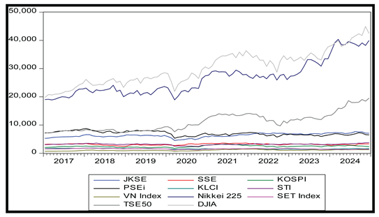 |
Appendix C
| Results of the Stationarity Test for Monthly Stock Market Indices in Asia and the United States, January 2017 – December 2024. Indonesia (^JKSE) | ||||
| First Difference | ||||
| Null Hypothesis: D(JKSE) has a unit root | ||||
| Exogenous: Constant | ||||
| Lag Length: 0 (Automatic - based on SIC, maxlag=11) | ||||
| t-Statistic | Prob.* | |||
| Augmented Dickey-Fuller test statistic | -8.402967 | 0.0000 | ||
| Test critical values: | 1% level | -3.501445 | ||
| 5% level | -2.892536 | |||
| 10% level | -2.583371 | |||
| *MacKinnon (1996) one-sided p-values. | ||||
| China (^SSE) | ||||
| First Difference | ||||
| Null Hypothesis: D(SSE) has a unit root | ||||
| Exogenous: Constant | ||||
| Lag Length: 0 (Automatic - based on SIC, maxlag=11) | ||||
| t-Statistic | Prob.* | |||
| Augmented Dickey-Fuller test statistic | -10.51872 | 0.0000 | ||
| Test critical values: | 1% level | -3.501445 | ||
| 5% level | -2.892536 | |||
| 10% level | -2.583371 | |||
| *MacKinnon (1996) one-sided p-values. | ||||
| South Korea (^KOSPI) | ||||
| First Difference | ||||
| Null Hypothesis: D(KOSPI) has a unit root | ||||
| Exogenous: Constant | ||||
| Lag Length: 0 (Automatic - based on SIC, maxlag=11) | ||||
| t-Statistic | Prob.* | |||
| Augmented Dickey-Fuller test statistic | -10.28708 | 0.0000 | ||
| Test critical values: | 1% level | -3.501445 | ||
| 5% level | -2.892536 | |||
| 10% level | -2.583371 | |||
| *MacKinnon (1996) one-sided p-values. | ||||
| Philippines (^PSEi) | ||||
| First Difference | ||||
| Null Hypothesis: D(PSEI) has a unit root | ||||
| Exogenous: Constant | ||||
| Lag Length: 0 (Automatic - based on SIC, maxlag=11) | ||||
| t-Statistic | Prob.* | |||
| Augmented Dickey-Fuller test statistic | -9.998390 | 0.0000 | ||
| Test critical values: | 1% level | -3.501445 | ||
| 5% level | -2.892536 | |||
| 10% level | -2.583371 | |||
| *MacKinnon (1996) one-sided p-values. | ||||
| Malaysia (^KLCI) | ||||
| First Difference | ||||
| Null Hypothesis: D(KLCI) has a unit root | ||||
| Exogenous: Constant | ||||
| Lag Length: 0 (Automatic - based on SIC, maxlag=11) | ||||
| t-Statistic | Prob.* | |||
| Augmented Dickey-Fuller test statistic | -9.825738 | 0.0000 | ||
| Test critical values: | 1% level | -3.501445 | ||
| 5% level | -2.892536 | |||
| 10% level | -2.583371 | |||
| *MacKinnon (1996) one-sided p-values. | ||||
| Singapore (^STI) | ||||
| First Difference | ||||
| Null Hypothesis: D(STI) has a unit root | ||||
| Exogenous: Constant | ||||
| Lag Length: 0 (Automatic - based on SIC, maxlag=11) | ||||
| t-Statistic | Prob.* | |||
| Augmented Dickey-Fuller test statistic | -11.68863 | 0.0000 | ||
| Test critical values: | 1% level | -3.501445 | ||
| 5% level | -2.892536 | |||
| 10% level | -2.583371 | |||
| *MacKinnon (1996) one-sided p-values. | ||||
| Vietnam (^VN Index) | ||||
| First Difference | ||||
| Null Hypothesis: D(VN_INDEX) has a unit root | ||||
| Exogenous: Constant | ||||
| Lag Length: 0 (Automatic - based on SIC, maxlag=11) | ||||
| t-Statistic | Prob.* | |||
| Augmented Dickey-Fuller test statistic | -8.895285 | 0.0000 | ||
| Test critical values: | 1% level | -3.501445 | ||
| 5% level | -2.892536 | |||
| 10% level | -2.583371 | |||
| *MacKinnon (1996) one-sided p-values. | ||||
| Japan (^Nikkei 225) | ||||
| First Difference | ||||
| Null Hypothesis: D(NIKKEI_225) has a unit root | ||||
| Exogenous: Constant | ||||
| Lag Length: 0 (Automatic - based on SIC, maxlag=11) | ||||
| t-Statistic | Prob.* | |||
| Augmented Dickey-Fuller test statistic | -9.602110 | 0.0000 | ||
| Test critical values: | 1% level | -3.501445 | ||
| 5% level | -2.892536 | |||
| 10% level | -2.583371 | |||
| *MacKinnon (1996) one-sided p-values. | ||||
| Thailand (^SET Index) | ||||
| First Difference | ||||
| Null Hypothesis: D(SET_INDEX) has a unit root | ||||
| Exogenous: Constant | ||||
| Lag Length: 0 (Automatic - based on SIC, maxlag=11) | ||||
| t-Statistic | Prob.* | |||
| Augmented Dickey-Fuller test statistic | -9.226301 | 0.0000 | ||
| Test critical values: | 1% level | -3.501445 | ||
| 5% level | -2.892536 | |||
| 10% level | -2.583371 | |||
| *MacKinnon (1996) one-sided p-values. | ||||
| Taiwan (^TSE50) | ||||
| First Difference | ||||
| Null Hypothesis: D(TSE50) has a unit root | ||||
| Exogenous: Constant | ||||
| Lag Length: 0 (Automatic - based on SIC, maxlag=11) | ||||
| t-Statistic | Prob.* | |||
| Augmented Dickey-Fuller test statistic | -10.31524 | 0.0000 | ||
| Test critical values: | 1% level | -3.501445 | ||
| 5% level | -2.892536 | |||
| 10% level | -2.583371 | |||
| *MacKinnon (1996) one-sided p-values. | ||||
| USA (^DJIA) | ||||
| First Difference | ||||
| Null Hypothesis: D(DJIA) has a unit root | ||||
| Exogenous: Constant | ||||
| Lag Length: 0 (Automatic - based on SIC, maxlag=11) | ||||
| t-Statistic | Prob.* | |||
| Augmented Dickey-Fuller test statistic | -11.35663 | 0.0000 | ||
| Test critical values: | 1% level | -3.501445 | ||
| 5% level | -2.892536 | |||
| 10% level | -2.583371 | |||
| *MacKinnon (1996) one-sided p-values. | ||||
Appendix D
| Results of the Causality Test for Monthly Stock Market Indices in Asia and the United States, January 2017 – December 2024 | |||
| Pairwise Granger Causality Tests | |||
| Date: 05/24/25 Time: 01:19 | |||
| Sample: 2017M01 2024M12 | |||
| Lags: 6 | |||
| Null Hypothesis: | Obs | F-Statistic | Prob. |
| SSE does not Granger Cause JKSE | 90 | 1.04890 | 0.4007 |
| JKSE does not Granger Cause SSE | 1.26469 | 0.2836 | |
| KOSPI does not Granger Cause JKSE | 90 | 1.22078 | 0.3049 |
| JKSE does not Granger Cause KOSPI | 0.76641 | 0.5986 | |
| PSEI does not Granger Cause JKSE | 90 | 1.79071 | 0.1120 |
| JKSE does not Granger Cause PSEI | 1.33869 | 0.2504 | |
| KLCI does not Granger Cause JKSE | 90 | 0.42595 | 0.8595 |
| JKSE does not Granger Cause KLCI | 0.31186 | 0.9290 | |
| STI does not Granger Cause JKSE | 90 | 1.06048 | 0.3936 |
| JKSE does not Granger Cause STI | 2.67944 | 0.0205 | |
| VN_INDEX does not Granger Cause JKSE | 90 | 1.21936 | 0.3056 |
| JKSE does not Granger Cause VN_INDEX | 1.84260 | 0.1018 | |
| NIKKEI_225 does not Granger Cause JKSE | 90 | 1.71819 | 0.1280 |
| JKSE does not Granger Cause NIKKEI_225 | 0.92705 | 0.4805 | |
| SET_INDEX does not Granger Cause JKSE | 90 | 0.80351 | 0.5702 |
| JKSE does not Granger Cause SET_INDEX | 1.32770 | 0.2551 | |
| TSE50 does not Granger Cause JKSE | 90 | 0.81809 | 0.5592 |
| JKSE does not Granger Cause TSE50 | 0.35681 | 0.9038 | |
| DJIA does not Granger Cause JKSE | 90 | 1.87834 | 0.0952 |
| JKSE does not Granger Cause DJIA | 1.04197 | 0.4050 | |
| KOSPI does not Granger Cause SSE | 90 | 1.90570 | 0.0905 |
| SSE does not Granger Cause KOSPI | 1.44357 | 0.2091 | |
| PSEI does not Granger Cause SSE | 90 | 3.00599 | 0.0108 |
| SSE does not Granger Cause PSEI | 0.88634 | 0.5092 | |
| KLCI does not Granger Cause SSE | 90 | 1.23090 | 0.2999 |
| SSE does not Granger Cause KLCI | 1.07544 | 0.3846 | |
| STI does not Granger Cause SSE | 90 | 2.55813 | 0.0260 |
| SSE does not Granger Cause STI | 0.71971 | 0.6349 | |
| VN_INDEX does not Granger Cause SSE | 90 | 1.63816 | 0.1480 |
| SSE does not Granger Cause VN_INDEX | 1.39061 | 0.2292 | |
| NIKKEI_225 does not Granger Cause SSE | 90 | 2.61074 | 0.0234 |
| SSE does not Granger Cause NIKKEI_225 | 1.25959 | 0.2860 | |
| SET_INDEX does not Granger Cause SSE | 90 | 1.99215 | 0.0769 |
| SSE does not Granger Cause SET_INDEX | 1.39897 | 0.2259 | |
| TSE50 does not Granger Cause SSE | 90 | 1.10448 | 0.3676 |
| SSE does not Granger Cause TSE50 | 0.87498 | 0.5173 | |
| DJIA does not Granger Cause SSE | 90 | 0.91327 | 0.4901 |
| SSE does not Granger Cause DJIA | 2.70711 | 0.0194 | |
| PSEI does not Granger Cause KOSPI | 90 | 1.75786 | 0.1190 |
| KOSPI does not Granger Cause PSEI | 0.55512 | 0.7645 | |
| KLCI does not Granger Cause KOSPI | 90 | 1.49072 | 0.1925 |
| KOSPI does not Granger Cause KLCI | 0.59198 | 0.7358 | |
| STI does not Granger Cause KOSPI | 90 | 3.09357 | 0.0091 |
| KOSPI does not Granger Cause STI | 0.64056 | 0.6974 | |
| VN_INDEX does not Granger Cause KOSPI | 90 | 0.51647 | 0.7941 |
| KOSPI does not Granger Cause VN_INDEX | 3.03899 | 0.0101 | |
| NIKKEI_225 does not Granger Cause KOSPI | 90 | 0.27098 | 0.9489 |
| KOSPI does not Granger Cause NIKKEI_225 | 1.35611 | 0.2431 | |
| SET_INDEX does not Granger Cause KOSPI | 90 | 1.23741 | 0.2967 |
| KOSPI does not Granger Cause SET_INDEX | 0.52910 | 0.7845 | |
| TSE50 does not Granger Cause KOSPI | 90 | 0.67793 | 0.6678 |
| KOSPI does not Granger Cause TSE50 | 1.67423 | 0.1387 | |
| DJIA does not Granger Cause KOSPI | 90 | 0.34915 | 0.9083 |
| KOSPI does not Granger Cause DJIA | 0.76083 | 0.6029 | |
| KLCI does not Granger Cause PSEI | 90 | 3.27636 | 0.0064 |
| PSEI does not Granger Cause KLCI | 1.09267 | 0.3744 | |
| STI does not Granger Cause PSEI | 90 | 0.51439 | 0.7957 |
| PSEI does not Granger Cause STI | 2.20541 | 0.0513 | |
| VN_INDEX does not Granger Cause PSEI | 90 | 0.52427 | 0.7882 |
| PSEI does not Granger Cause VN_INDEX | 1.04075 | 0.4057 | |
| NIKKEI_225 does not Granger Cause PSEI | 90 | 0.82118 | 0.5569 |
| PSEI does not Granger Cause NIKKEI_225 | 0.85395 | 0.5326 | |
| SET_INDEX does not Granger Cause PSEI | 90 | 0.64128 | 0.6968 |
| PSEI does not Granger Cause SET_INDEX | 0.77169 | 0.5945 | |
| TSE50 does not Granger Cause PSEI | 90 | 0.74775 | 0.6130 |
| PSEI does not Granger Cause TSE50 | 1.34714 | 0.2468 | |
| DJIA does not Granger Cause PSEI | 90 | 1.47851 | 0.1967 |
| PSEI does not Granger Cause DJIA | 1.54456 | 0.1750 | |
| STI does not Granger Cause KLCI | 90 | 0.86622 | 0.5237 |
| KLCI does not Granger Cause STI | 1.28196 | 0.2755 | |
| VN_INDEX does not Granger Cause KLCI | 90 | 1.04115 | 0.4055 |
| KLCI does not Granger Cause VN_INDEX | 1.30903 | 0.2633 | |
| NIKKEI_225 does not Granger Cause KLCI | 90 | 1.01429 | 0.4224 |
| KLCI does not Granger Cause NIKKEI_225 | 0.85022 | 0.5354 | |
| SET_INDEX does not Granger Cause KLCI | 90 | 1.56822 | 0.1678 |
| KLCI does not Granger Cause SET_INDEX | 3.09626 | 0.0091 | |
| TSE50 does not Granger Cause KLCI | 90 | 1.09894 | 0.3708 |
| KLCI does not Granger Cause TSE50 | 0.95706 | 0.4600 | |
| DJIA does not Granger Cause KLCI | 90 | 0.77119 | 0.5949 |
| KLCI does not Granger Cause DJIA | 0.18362 | 0.9806 | |
| VN_INDEX does not Granger Cause STI | 90 | 0.48931 | 0.8144 |
| STI does not Granger Cause VN_INDEX | 0.63329 | 0.7032 | |
| NIKKEI_225 does not Granger Cause STI | 90 | 1.19813 | 0.3164 |
| STI does not Granger Cause NIKKEI_225 | 1.28320 | 0.2750 | |
| SET_INDEX does not Granger Cause STI | 90 | 1.96575 | 0.0809 |
| STI does not Granger Cause SET_INDEX | 0.50628 | 0.8018 | |
| TSE50 does not Granger Cause STI | 90 | 1.15996 | 0.3365 |
| STI does not Granger Cause TSE50 | 1.15798 | 0.3376 | |
| DJIA does not Granger Cause STI | 90 | 0.79608 | 0.5759 |
| STI does not Granger Cause DJIA | 1.14493 | 0.3447 | |
| NIKKEI_225 does not Granger Cause VN_INDEX | 90 | 1.08927 | 0.3764 |
| VN_INDEX does not Granger Cause NIKKEI_225 | 1.16848 | 0.3320 | |
| SET_INDEX does not Granger Cause VN_INDEX | 90 | 1.99992 | 0.0758 |
| VN_INDEX does not Granger Cause SET_INDEX | 0.54390 | 0.7732 | |
| TSE50 does not Granger Cause VN_INDEX | 90 | 1.07069 | 0.3875 |
| VN_INDEX does not Granger Cause TSE50 | 2.06600 | 0.0669 | |
| DJIA does not Granger Cause VN_INDEX | 90 | 1.82599 | 0.1050 |
| VN_INDEX does not Granger Cause DJIA | 1.27642 | 0.2781 | |
| SET_INDEX does not Granger Cause NIKKEI_225 | 90 | 1.09992 | 0.3702 |
| NIKKEI_225 does not Granger Cause SET_INDEX | 0.75210 | 0.6096 | |
| TSE50 does not Granger Cause NIKKEI_225 | 90 | 0.84366 | 0.5402 |
| NIKKEI_225 does not Granger Cause TSE50 | 1.49040 | 0.1926 | |
| DJIA does not Granger Cause NIKKEI_225 | 90 | 0.69548 | 0.6540 |
| NIKKEI_225 does not Granger Cause DJIA | 1.85121 | 0.1002 | |
| TSE50 does not Granger Cause SET_INDEX | 90 | 0.99390 | 0.4355 |
| SET_INDEX does not Granger Cause TSE50 | 3.46395 | 0.0044 | |
| DJIA does not Granger Cause SET_INDEX | 90 | 0.45743 | 0.8376 |
| SET_INDEX does not Granger Cause DJIA | 1.71045 | 0.1298 | |
| DJIA does not Granger Cause TSE50 | 90 | 2.12618 | 0.0597 |
| TSE50 does not Granger Cause DJIA | 0.98065 | 0.4442 | |
Appendix E
| Cointegration Test of Monthly Stock Market Indices in Asia and the United States: January 2017 – December 2024 | |||||
| Date: 05/24/25 Time: 00:03 | |||||
| Sample: 2017M01 2024M12 | |||||
| Included observations: 92 | |||||
| Series: D(JKSE) D(SSE) D(KOSPI) D(PSEI) D(KLCI) D(STI) D(VN_INDEX) D(NIKKEI_225) D(SET_INDEX) D(TSE50) D(DJIA) | |||||
| Lags interval: 1 to 2 | |||||
| Selected (0.05 level*) Number of Cointegrating Relations by Model | |||||
| Data Trend: | None | None | Linear | Linear | Quadratic |
| Test Type | No Intercept | Intercept | Intercept | Intercept | Intercept |
| No Trend | No Trend | No Trend | Trend | Trend | |
| Trace | 11 | 11 | 11 | 10 | 11 |
| Max-Eig | 1 | 1 | 1 | 1 | 1 |
| *Critical values based on MacKinnon-Haug-Michelis (1999) | |||||
| Information Criteria by Rank and Model | |||||
| Data Trend: | None | None | Linear | Linear | Quadratic |
| Rank or | No Intercept | Intercept | Intercept | Intercept | Intercept |
| No. of CEs | No Trend | No Trend | No Trend | Trend | Trend |
| Log Likelihood by Rank (rows) and Model (columns) | |||||
| 0 | -6541.032 | -6541.032 | -6540.824 | -6540.824 | -6540.437 |
| 1 | -6502.544 | -6495.929 | -6495.731 | -6493.665 | -6493.278 |
| 2 | -6473.627 | -6465.171 | -6465.001 | -6462.622 | -6462.261 |
| 3 | -6446.094 | -6436.373 | -6436.204 | -6433.301 | -6432.940 |
| 4 | -6421.048 | -6411.288 | -6411.166 | -6407.894 | -6407.637 |
| 5 | -6398.777 | -6387.780 | -6387.689 | -6383.415 | -6383.262 |
| 6 | -6379.113 | -6368.055 | -6367.983 | -6363.092 | -6362.960 |
| 7 | -6366.357 | -6353.695 | -6353.628 | -6346.992 | -6346.936 |
| 8 | -6355.330 | -6341.376 | -6341.309 | -6332.760 | -6332.712 |
| 9 | -6346.964 | -6332.983 | -6332.953 | -6323.576 | -6323.547 |
| 10 | -6340.839 | -6325.643 | -6325.615 | -6315.523 | -6315.521 |
| 11 | -6335.391 | -6319.846 | -6319.846 | -6309.677 | -6309.677 |
| Akaike Information Criteria by Rank (rows) and Model (columns) | |||||
| 0 | 147.4572 | 147.4572 | 147.6918 | 147.6918 | 147.9225 |
| 1 | 147.0988 | 146.9767 | 147.1898 | 147.1666 | 147.3756 |
| 2 | 146.9484 | 146.8081 | 147.0000 | 146.9918 | 147.1796 |
| 3 | 146.8281 | 146.6820 | 146.8523 | 146.8544 | 147.0204 |
| 4 | 146.7619 | 146.6367 | 146.7862 | 146.8021 | 146.9486 |
| 5 | 146.7560 | 146.6257* | 146.7541 | 146.7699 | 146.8970 |
| 6 | 146.8068 | 146.6969 | 146.8040 | 146.8281 | 146.9339 |
| 7 | 147.0078 | 146.8847 | 146.9702 | 146.9781 | 147.0638 |
| 8 | 147.2463 | 147.1169 | 147.1806 | 147.1687 | 147.2329 |
| 9 | 147.5427 | 147.4344 | 147.4772 | 147.4690 | 147.5119 |
| 10 | 147.8878 | 147.7749 | 147.7960 | 147.7940 | 147.8157 |
| 11 | 148.2476 | 148.1488 | 148.1488 | 148.1669 | 148.1669 |
| Schwarz Criteria by Rank (rows) and Model (columns) | |||||
| 0 | 154.0906* | 154.0906* | 154.6267 | 154.6267 | 155.1590 |
| 1 | 154.3352 | 154.2406 | 154.7278 | 154.7320 | 155.2151 |
| 2 | 154.7879 | 154.7024 | 155.1410 | 155.1876 | 155.6221 |
| 3 | 155.2706 | 155.2068 | 155.5963 | 155.6806 | 156.0660 |
| 4 | 155.8075 | 155.7919 | 156.1333 | 156.2588 | 156.5972 |
| 5 | 156.4046 | 156.4113 | 156.7042 | 156.8570 | 157.1486 |
| 6 | 157.0584 | 157.1129 | 157.3571 | 157.5457 | 157.7886 |
| 7 | 157.8624 | 157.9312 | 158.1264 | 158.3261 | 158.5215 |
| 8 | 158.7040 | 158.7938 | 158.9398 | 159.1472 | 159.2936 |
| 9 | 159.6034 | 159.7418 | 159.8395 | 160.0780 | 160.1756 |
| 10 | 160.5516 | 160.7127 | 160.7613 | 161.0334 | 161.0825 |
| 11 | 161.5144 | 161.7171 | 161.7171 | 162.0367 | 162.0367 |
Appendix F
| VECM Estimation Results for Monthly Stock Indices in Asia and the United States: January 2017 – December 2024 | |||||||||||
| Vector Error Correction Estimates | |||||||||||
| Date: 05/29/25 Time: 11:11 | |||||||||||
| Sample (adjusted): 2017M08 2024M12 | |||||||||||
| Included observations: 89 after adjustments | |||||||||||
| Standard errors in ( ) & t-statistics in [ ] | |||||||||||
| Cointegrating Eq: | CointEq1 | ||||||||||
| D(JKSE(-1)) | 1.000000 | ||||||||||
| D(SSE(-1)) | -1.209627 | ||||||||||
| (0.86787) | |||||||||||
| [-1.39379] | |||||||||||
| D(KOSPI(-1)) | 0.994775 | ||||||||||
| (1.05879) | |||||||||||
| [ 0.93954] | |||||||||||
| D(KLCI(-1)) | 4.837238 | ||||||||||
| (2.31595) | |||||||||||
| [ 2.08866] | |||||||||||
| D(PSEI(-1)) | -0.767616 | ||||||||||
| (0.45794) | |||||||||||
| [-1.67622] | |||||||||||
| D(STI(-1)) | 8.091343 | ||||||||||
| (1.35641) | |||||||||||
| [ 5.96527] | |||||||||||
| D(SET_INDEX(-1)) | -19.26842 | ||||||||||
| (2.17870) | |||||||||||
| [-8.84400] | |||||||||||
| D(NIKKEI_225(-1)) | -0.685003 | ||||||||||
| (0.10040) | |||||||||||
| [-6.82298] | |||||||||||
| D(VN_INDEX(-1)) | 5.358982 | ||||||||||
| (1.31574) | |||||||||||
| [ 4.07298] | |||||||||||
| D(TSE50(-1)) | -0.406717 | ||||||||||
| (0.18692) | |||||||||||
| [-2.17586] | |||||||||||
| D(DJIA(-1)) | 0.233440 | ||||||||||
| (0.15085) | |||||||||||
| [ 1.54746] | |||||||||||
| C | 26.64729 | ||||||||||
| (38.1307) | |||||||||||
| [ 0.69884] | |||||||||||
| Error Correction: | D(JKSE,2) | D(SSE,2) | D(KOSPI,2) | D(KLCI,2) | D(PSEI,2) | D(STI,2) | D(SET_ INDEX,2) |
D(NIKKEI_ 225,2) |
D(VN_INDEX,2) | D(TSE50,2) | D(DJIA,2) |
| CointEq1 | -0.259415 | -0.021901 | -0.009902 | 0.016710 | -0.182894 | -0.063778 | 0.041426 | 0.487340 | -0.086748 | -0.018921 | -0.139867 |
| (0.09490) | (0.05793) | (0.05866) | (0.01801) | (0.12837) | (0.04832) | (0.02361) | (0.60406) | (0.02670) | (0.26535) | (0.54060) | |
| [-2.73368] | [-0.37808] | [-0.16881] | [ 0.92786] | [-1.42480] | [-1.31985] | [ 1.75472] | [ 0.80677] | [-3.24896] | [-0.07130] | [-0.25873] | |
| D(JKSE(-1),2) | -0.824091 | -0.186560 | -0.097845 | -0.044698 | -0.284667 | -0.044107 | -0.066011 | 0.075456 | 0.060456 | -1.231863 | 1.290881 |
| (0.21462) | (0.13100) | (0.13266) | (0.04073) | (0.29031) | (0.10929) | (0.05339) | (1.36616) | (0.06039) | (0.60013) | (1.22262) | |
| [-3.83980] | [-1.42407] | [-0.73755] | [-1.09745] | [-0.98055] | [-0.40359] | [-1.23633] | [ 0.05523] | [ 1.00117] | [-2.05267] | [ 1.05583] | |
| D(JKSE(-2),2) | -0.320959 | -0.041691 | -0.067374 | -0.033342 | 0.098525 | -0.057939 | -0.210676 | 1.661308 | 0.005157 | -1.237024 | -0.421899 |
| (0.26030) | (0.15889) | (0.16090) | (0.04940) | (0.35210) | (0.13255) | (0.06476) | (1.65692) | (0.07324) | (0.72786) | (1.48284) | |
| [-1.23305] | [-0.26239] | [-0.41874] | [-0.67498] | [ 0.27982] | [-0.43712] | [-3.25337] | [ 1.00265] | [ 0.07041] | [-1.69955] | [-0.28452] | |
| D(JKSE(-3),2) | -0.547240 | 0.105626 | 0.055456 | 0.035844 | -0.029267 | 0.085208 | -0.028156 | 2.609528 | 0.097959 | -0.931833 | 3.290025 |
| (0.26466) | (0.16155) | (0.16359) | (0.05022) | (0.35800) | (0.13477) | (0.06584) | (1.68468) | (0.07446) | (0.74005) | (1.50767) | |
| [-2.06774] | [ 0.65384] | [ 0.33899] | [ 0.71368] | [-0.08175] | [ 0.63226] | [-0.42763] | [ 1.54898] | [ 1.31551] | [-1.25915] | [ 2.18219] | |
| D(JKSE(-4),2) | 0.187224 | 0.425739 | 0.369960 | 0.157982 | 0.981442 | 0.578794 | 0.122472 | 5.434149 | 0.199565 | 1.285053 | 4.213384 |
| (0.29754) | (0.18162) | (0.18392) | (0.05647) | (0.40248) | (0.15151) | (0.07402) | (1.89401) | (0.08372) | (0.83200) | (1.69501) | |
| [ 0.62924] | [ 2.34410] | [ 2.01155] | [ 2.79787] | [ 2.43847] | [ 3.82012] | [ 1.65453] | [ 2.86912] | [ 2.38379] | [ 1.54453] | [ 2.48575] | |
| D(JKSE(-5),2) | -0.338052 | 0.124572 | -0.057635 | 0.016455 | -0.293186 | 0.302631 | 0.007347 | 0.801650 | 0.011382 | -0.024789 | 2.360474 |
| (0.23238) | (0.14185) | (0.14364) | (0.04410) | (0.31434) | (0.11833) | (0.05781) | (1.47923) | (0.06538) | (0.64980) | (1.32381) | |
| [-1.45473] | [ 0.87821] | [-0.40124] | [ 0.37313] | [-0.93270] | [ 2.55748] | [ 0.12708] | [ 0.54194] | [ 0.17408] | [-0.03815] | [ 1.78309] | |
| D(SSE(-1),2) | -1.128565 | -0.960117 | -0.352274 | -0.416988 | -1.933574 | -0.695912 | -0.261640 | -0.860236 | -0.195544 | -2.201188 | -3.462462 |
| (0.36161) | (0.22073) | (0.22352) | (0.06862) | (0.48915) | (0.18414) | (0.08996) | (2.30184) | (0.10174) | (1.01116) | (2.06000) | |
| [-3.12094] | [-4.34973] | [-1.57602] | [-6.07645] | [-3.95294] | [-3.77931] | [-2.90836] | [-0.37372] | [-1.92192] | [-2.17690] | [-1.68081] | |
| D(SSE(-2),2) | -0.045075 | -0.372727 | 0.209287 | -0.138295 | -0.113220 | 0.068770 | -0.121824 | 3.931432 | 0.177897 | 0.598112 | 2.135868 |
| (0.32789) | (0.20015) | (0.20268) | (0.06222) | (0.44353) | (0.16697) | (0.08157) | (2.08719) | (0.09226) | (0.91686) | (1.86789) | |
| [-0.13747] | [-1.86227] | [ 1.03261] | [-2.22253] | [-0.25527] | [ 0.41188] | [-1.49346] | [ 1.88360] | [ 1.92829] | [ 0.65235] | [ 1.14346] | |
| D(SSE(-3),2) | -0.222957 | -0.418032 | -0.164023 | -0.155916 | -0.421780 | -0.202009 | -0.236922 | 0.358317 | -0.014904 | -0.038839 | -3.499831 |
| (0.29838) | (0.18213) | (0.18443) | (0.05662) | (0.40361) | (0.15194) | (0.07423) | (1.89933) | (0.08395) | (0.83434) | (1.69977) | |
| [-0.74723] | [-2.29522] | [-0.88933] | [-2.75355] | [-1.04501] | [-1.32955] | [-3.19172] | [ 0.18865] | [-0.17753] | [-0.04655] | [-2.05900] | |
| D(SSE(-4),2) | -0.553669 | -0.601685 | -0.267625 | -0.230535 | -0.961927 | -0.278678 | -0.067770 | 1.212298 | -0.060624 | -1.711061 | -0.046068 |
| (0.34327) | (0.20953) | (0.21218) | (0.06514) | (0.46433) | (0.17480) | (0.08540) | (2.18507) | (0.09658) | (0.95986) | (1.95549) | |
| [-1.61295] | [-2.87157] | [-1.26131] | [-3.53895] | [-2.07163] | [-1.59431] | [-0.79358] | [ 0.55481] | [-0.62769] | [-1.78262] | [-0.02356] | |
| D(SSE(-5),2) | 0.139168 | -0.205520 | 0.053888 | -0.092264 | 0.312597 | 0.150179 | -0.148185 | 2.943245 | -0.051780 | -0.514371 | 0.943297 |
| (0.28516) | (0.17406) | (0.17626) | (0.05411) | (0.38573) | (0.14521) | (0.07094) | (1.81517) | (0.08023) | (0.79737) | (1.62445) | |
| [ 0.48804] | [-1.18074] | [ 0.30573] | [-1.70498] | [ 0.81041] | [ 1.03426] | [-2.08885] | [ 1.62147] | [-0.64537] | [-0.64509] | [ 0.58069] | |
| D(KOSPI(-1),2) | -0.636647 | -0.333536 | -0.956130 | -0.372849 | -1.553881 | 0.012064 | -0.297644 | 0.256759 | -0.281251 | -2.379336 | -2.431011 |
| (0.51138) | (0.31215) | (0.31610) | (0.09705) | (0.69174) | (0.26040) | (0.12722) | (3.25522) | (0.14388) | (1.42995) | (2.91320) | |
| [-1.24495] | [-1.06851] | [-3.02479] | [-3.84198] | [-2.24633] | [ 0.04633] | [-2.33957] | [ 0.07888] | [-1.95470] | [-1.66392] | [-0.83448] | |
| D(KOSPI(-2),2) | 0.324060 | 0.409433 | -0.430766 | 0.110227 | 0.279557 | 0.466109 | -0.005552 | 4.505500 | -0.029945 | -0.398412 | 0.606699 |
| (0.60307) | (0.36812) | (0.37277) | (0.11445) | (0.81577) | (0.30709) | (0.15003) | (3.83887) | (0.16968) | (1.68635) | (3.43553) | |
| [ 0.53735] | [ 1.11223] | [-1.15557] | [ 0.96313] | [ 0.34269] | [ 1.51781] | [-0.03700] | [ 1.17365] | [-0.17648] | [-0.23626] | [ 0.17660] | |
| D(KOSPI(-3),2) | 1.114984 | 0.602012 | 0.190752 | 0.355283 | 0.920219 | 0.713352 | 0.304009 | 7.328867 | 0.028750 | 2.050680 | 8.982405 |
| (0.61649) | (0.37631) | (0.38107) | (0.11699) | (0.83392) | (0.31392) | (0.15337) | (3.92427) | (0.17346) | (1.72386) | (3.51196) | |
| [ 1.80861] | [ 1.59978] | [ 0.50057] | [ 3.03681] | [ 1.10349] | [ 2.27237] | [ 1.98220] | [ 1.86758] | [ 0.16575] | [ 1.18959] | [ 2.55766] | |
| D(KOSPI(-4),2) | 1.297821 | 0.251617 | 0.250472 | 0.392750 | 1.167364 | 0.401511 | 0.253117 | 1.404245 | -0.135642 | 2.469351 | 1.192167 |
| (0.60398) | (0.36868) | (0.37334) | (0.11462) | (0.81701) | (0.30756) | (0.15026) | (3.84468) | (0.16994) | (1.68890) | (3.44073) | |
| [ 2.14877] | [ 0.68249] | [ 0.67090] | [ 3.42656] | [ 1.42883] | [ 1.30548] | [ 1.68454] | [ 0.36524] | [-0.79818] | [ 1.46211] | [ 0.34649] | |
| D(KOSPI(-5),2) | 0.700726 | 0.321348 | 0.149113 | 0.333940 | 1.318312 | 0.442526 | 0.466342 | -1.347065 | -0.018935 | -0.145499 | 2.585452 |
| (0.52822) | (0.32243) | (0.32651) | (0.10024) | (0.71452) | (0.26898) | (0.13141) | (3.36239) | (0.14862) | (1.47703) | (3.00911) | |
| [ 1.32658] | [ 0.99665] | [ 0.45669] | [ 3.33137] | [ 1.84504] | [ 1.64523] | [ 3.54876] | [-0.40063] | [-0.12741] | [-0.09851] | [ 0.85921] | |
| D(KLCI(-1),2) | 1.338162 | 0.754509 | -0.047474 | -0.995492 | 0.320321 | 0.399533 | -0.318522 | -2.934466 | 0.574538 | 0.139747 | -3.041143 |
| (1.01586) | (0.62009) | (0.62793) | (0.19278) | (1.37414) | (0.51729) | (0.25273) | (6.46648) | (0.28583) | (2.84060) | (5.78707) | |
| [ 1.31727] | [ 1.21678] | [-0.07560] | [-5.16383] | [ 0.23311] | [ 0.77236] | [-1.26035] | [-0.45380] | [ 2.01010] | [ 0.04920] | [-0.52551] | |
| D(KLCI(-2),2) | 1.278498 | 0.062149 | -0.520767 | -0.958121 | -1.453217 | -0.657230 | -0.635803 | -11.09749 | 0.147747 | -0.193494 | -11.51114 |
| (1.15807) | (0.70689) | (0.71583) | (0.21977) | (1.56651) | (0.58970) | (0.28810) | (7.37170) | (0.32584) | (3.23825) | (6.59718) | |
| [ 1.10399] | [ 0.08792] | [-0.72750] | [-4.35968] | [-0.92768] | [-1.11451] | [-2.20686] | [-1.50542] | [ 0.45344] | [-0.05975] | [-1.74486] | |
| D(KLCI(-3),2) | -0.209841 | -0.738699 | -1.041537 | -1.039874 | -1.607948 | -1.803739 | -0.724920 | -16.94097 | -0.209395 | -3.320355 | -16.30095 |
| (1.20564) | (0.73593) | (0.74524) | (0.22880) | (1.63086) | (0.61393) | (0.29994) | (7.67455) | (0.33922) | (3.37129) | (6.86821) | |
| [-0.17405] | [-1.00376] | [-1.39759] | [-4.54495] | [-0.98595] | [-2.93802] | [-2.41689] | [-2.20742] | [-0.61728] | [-0.98489] | [-2.37339] | |
| D(KLCI(-4),2) | 0.090709 | 0.033477 | -0.526649 | -0.783646 | 0.061785 | -0.220849 | -0.507460 | -9.274144 | -0.377832 | -1.633436 | -2.893645 |
| (1.13088) | (0.69030) | (0.69903) | (0.21461) | (1.52974) | (0.57586) | (0.28134) | (7.19867) | (0.31819) | (3.16224) | (6.44233) | |
| [ 0.08021] | [ 0.04850] | [-0.75340] | [-3.65148] | [ 0.04039] | [-0.38351] | [-1.80372] | [-1.28831] | [-1.18744] | [-0.51654] | [-0.44916] | |
| D(KLCI(-5),2) | -0.050102 | 0.243510 | 0.097610 | -0.494214 | -0.149732 | 0.111895 | -0.843582 | -2.135723 | -0.202799 | 2.584548 | -7.717223 |
| (0.89703) | (0.54756) | (0.55448) | (0.17023) | (1.21341) | (0.45678) | (0.22316) | (5.71009) | (0.25239) | (2.50833) | (5.11015) | |
| [-0.05585] | [ 0.44472] | [ 0.17604] | [-2.90318] | [-0.12340] | [ 0.24496] | [-3.78011] | [-0.37403] | [-0.80351] | [ 1.03038] | [-1.51018] | |
| D(PSEI(-1),2) | 0.506049 | 0.252733 | 0.249951 | 0.155143 | 0.093768 | 0.308793 | 0.160344 | 1.135903 | 0.017204 | 1.980481 | 1.153755 |
| (0.21262) | (0.12979) | (0.13143) | (0.04035) | (0.28761) | (0.10827) | (0.05290) | (1.35345) | (0.05982) | (0.59455) | (1.21125) | |
| [ 2.38004] | [ 1.94730] | [ 1.90182] | [ 3.84495] | [ 0.32602] | [ 2.85206] | [ 3.03130] | [ 0.83926] | [ 0.28758] | [ 3.33108] | [ 0.95253] | |
| D(PSEI(-2),2) | 0.289675 | 0.168612 | 0.110697 | 0.094695 | -0.092507 | 0.293849 | 0.220993 | -1.243962 | 0.002215 | 1.936560 | 1.752395 |
| (0.23605) | (0.14409) | (0.14591) | (0.04480) | (0.31931) | (0.12020) | (0.05872) | (1.50260) | (0.06642) | (0.66006) | (1.34472) | |
| [ 1.22717] | [ 1.17020] | [ 0.75867] | [ 2.11391] | [-0.28971] | [ 2.44465] | [ 3.76319] | [-0.82787] | [ 0.03336] | [ 2.93390] | [ 1.30316] | |
| D(PSEI(-3),2) | 0.247775 | 0.126190 | 0.031783 | -0.019122 | -0.055697 | 0.185887 | 0.117535 | -1.280238 | -0.048101 | 1.600249 | -0.815309 |
| (0.25625) | (0.15642) | (0.15840) | (0.04863) | (0.34663) | (0.13049) | (0.06375) | (1.63118) | (0.07210) | (0.71655) | (1.45980) | |
| [ 0.96691] | [ 0.80675] | [ 0.20065] | [-0.39321] | [-0.16068] | [ 1.42456] | [ 1.84367] | [-0.78485] | [-0.66714] | [ 2.23327] | [-0.55851] | |
| D(PSEI(-4),2) | -0.121241 | -0.139313 | -0.260612 | -0.069399 | -0.427484 | -0.064323 | 0.014357 | -2.249207 | -0.056693 | -0.317268 | -2.490594 |
| (0.22441) | (0.13698) | (0.13871) | (0.04259) | (0.30356) | (0.11427) | (0.05583) | (1.42850) | (0.06314) | (0.62751) | (1.27841) | |
| [-0.54026] | [-1.01701] | [-1.87876] | [-1.62957] | [-1.40823] | [-0.56288] | [ 0.25716] | [-1.57452] | [-0.89787] | [-0.50560] | [-1.94819] | |
| D(PSEI(-5),2) | 0.029136 | -0.093733 | -0.173918 | -0.056240 | -0.222927 | -0.164059 | -0.012110 | -1.243968 | -0.047612 | -0.793070 | -2.421171 |
| (0.15065) | (0.09196) | (0.09312) | (0.02859) | (0.20379) | (0.07672) | (0.03748) | (0.95899) | (0.04239) | (0.42127) | (0.85823) | |
| [ 0.19340] | [-1.01927] | [-1.86761] | [-1.96712] | [-1.09391] | [-2.13855] | [-0.32311] | [-1.29716] | [-1.12323] | [-1.88258] | [-2.82111] | |
| D(STI(-1),2) | 1.833011 | -0.150320 | -0.066901 | -0.126140 | 0.860285 | -0.959417 | -0.414000 | -6.089400 | 0.448668 | -0.213348 | -3.261284 |
| (0.72905) | (0.44502) | (0.45065) | (0.13835) | (0.98619) | (0.37124) | (0.18137) | (4.64081) | (0.20513) | (2.03862) | (4.15322) | |
| [ 2.51423] | [-0.33778] | [-0.14846] | [-0.91172] | [ 0.87234] | [-2.58433] | [-2.28258] | [-1.31214] | [ 2.18724] | [-0.10465] | [-0.78524] | |
| D(STI(-2),2) | 0.992676 | -0.072374 | 0.088985 | -0.391125 | 0.301095 | -1.053010 | -0.474228 | -6.205452 | 0.343849 | -0.445122 | -5.156381 |
| (0.72810) | (0.44444) | (0.45006) | (0.13817) | (0.98490) | (0.37076) | (0.18114) | (4.63475) | (0.20486) | (2.03596) | (4.14779) | |
| [ 1.36338] | [-0.16284] | [ 0.19772] | [-2.83068] | [ 0.30571] | [-2.84015] | [-2.61807] | [-1.33890] | [ 1.67845] | [-0.21863] | [-1.24316] | |
| D(STI(-3),2) | 1.129801 | 0.327372 | 0.248741 | -0.156835 | 0.652344 | -0.236432 | -0.226557 | -3.894269 | 0.384202 | 0.625517 | -0.954762 |
| (0.62445) | (0.38117) | (0.38599) | (0.11850) | (0.84469) | (0.31798) | (0.15535) | (3.97494) | (0.17570) | (1.74612) | (3.55730) | |
| [ 1.80928] | [ 0.85887] | [ 0.64443] | [-1.32347] | [ 0.77229] | [-0.74355] | [-1.45837] | [-0.97971] | [ 2.18673] | [ 0.35823] | [-0.26839] | |
| D(STI(-4),2) | 0.301196 | -0.083157 | -0.136723 | -0.249633 | 0.149947 | -0.268472 | -0.287325 | -6.421548 | 0.191898 | 0.556449 | -3.983414 |
| (0.55008) | (0.33577) | (0.34002) | (0.10439) | (0.74409) | (0.28011) | (0.13685) | (3.50154) | (0.15477) | (1.53816) | (3.13364) | |
| [ 0.54755] | [-0.24766] | [-0.40211] | [-2.39135] | [ 0.20152] | [-0.95846] | [-2.09959] | [-1.83392] | [ 1.23987] | [ 0.36176] | [-1.27118] | |
| D(STI(-5),2) | -1.273249 | -0.450888 | -0.439236 | -0.404009 | -2.021232 | -0.869953 | -0.298474 | -6.695764 | -0.048523 | -2.388694 | -7.232124 |
| (0.49952) | (0.30491) | (0.30877) | (0.09480) | (0.67570) | (0.25436) | (0.12427) | (3.17974) | (0.14055) | (1.39680) | (2.84565) | |
| [-2.54893] | [-1.47874] | [-1.42254] | [-4.26189] | [-2.99130] | [-3.42011] | [-2.40179] | [-2.10576] | [-0.34524] | [-1.71012] | [-2.54147] | |
| D(SET_INDEX(-1),2) | -3.687332 | 0.148625 | 0.237359 | 0.435480 | -2.228866 | -0.458183 | 0.329887 | 13.78839 | -1.038070 | 1.350458 | 5.113079 |
| (1.69509) | (1.03470) | (1.04778) | (0.32168) | (2.29294) | (0.86316) | (0.42171) | (10.7902) | (0.47694) | (4.73992) | (9.65648) | |
| [-2.17530] | [ 0.14364] | [ 0.22654] | [ 1.35376] | [-0.97206] | [-0.53082] | [ 0.78227] | [ 1.27787] | [-2.17653] | [ 0.28491] | [ 0.52950] | |
| D(SET_INDEX(-2),2) | -3.182557 | 0.544657 | 0.433066 | 0.708112 | -1.412598 | 1.218400 | 0.447847 | 15.38089 | -1.046233 | 2.099705 | 11.98501 |
| (1.61083) | (0.98326) | (0.99570) | (0.30569) | (2.17896) | (0.82026) | (0.40074) | (10.2538) | (0.45323) | (4.50430) | (9.17645) | |
| [-1.97572] | [ 0.55393] | [ 0.43494] | [ 2.31643] | [-0.64829] | [ 1.48539] | [ 1.11754] | [ 1.50002] | [-2.30840] | [ 0.46616] | [ 1.30606] | |
| D(SET_INDEX(-3),2) | -2.215811 | -0.108613 | 0.501354 | 0.677946 | -1.679908 | 0.743870 | 0.411984 | 9.125170 | -0.715028 | 4.462722 | 9.657331 |
| (1.42735) | (0.87126) | (0.88228) | (0.27087) | (1.93076) | (0.72683) | (0.35510) | (9.08583) | (0.40160) | (3.99124) | (8.13121) | |
| [-1.55240] | [-0.12466] | [ 0.56825] | [ 2.50283] | [-0.87007] | [ 1.02345] | [ 1.16021] | [ 1.00433] | [-1.78043] | [ 1.11813] | [ 1.18769] | |
| D(SET_INDEX(-4),2) | -1.189217 | -0.184363 | 0.430642 | 0.238108 | -2.419406 | -0.062077 | 0.304522 | 2.353285 | -0.610361 | 0.854497 | 7.802117 |
| (1.08830) | (0.66431) | (0.67271) | (0.20653) | (1.47214) | (0.55418) | (0.27075) | (6.92761) | (0.30621) | (3.04317) | (6.19974) | |
| [-1.09273] | [-0.27753] | [ 0.64016] | [ 1.15290] | [-1.64347] | [-0.11202] | [ 1.12475] | [ 0.33970] | [-1.99329] | [ 0.28079] | [ 1.25846] | |
| D(SET_INDEX(-5),2) | 0.081502 | 0.444828 | 0.050176 | 0.239271 | -0.136817 | 0.458814 | 0.397146 | -0.974721 | -0.034427 | 3.024871 | 4.843206 |
| (0.86453) | (0.52772) | (0.53439) | (0.16406) | (1.16945) | (0.44023) | (0.21508) | (5.50321) | (0.24325) | (2.41745) | (4.92500) | |
| [ 0.09427] | [ 0.84293] | [ 0.09389] | [ 1.45840] | [-0.11699] | [ 1.04221] | [ 1.84652] | [-0.17712] | [-0.14153] | [ 1.25126] | [ 0.98339] | |
| D(NIKKEI_225(-1),2) | -0.173297 | -0.016953 | -0.020155 | -0.015590 | -0.169753 | -0.082683 | 0.007163 | -0.626544 | -0.046930 | 0.028007 | -0.363714 |
| (0.06822) | (0.04164) | (0.04217) | (0.01295) | (0.09228) | (0.03474) | (0.01697) | (0.43424) | (0.01919) | (0.19075) | (0.38861) | |
| [-2.54038] | [-0.40713] | [-0.47799] | [-1.20429] | [-1.83960] | [-2.38025] | [ 0.42207] | [-1.44286] | [-2.44508] | [ 0.14682] | [-0.93593] | |
| D(NIKKEI_225(-2),2) | -0.123126 | -0.024886 | -0.035032 | -0.021615 | -0.190502 | -0.055671 | -0.004077 | -0.336367 | -0.033466 | -0.083448 | -0.277072 |
| (0.05535) | (0.03378) | (0.03421) | (0.01050) | (0.07487) | (0.02818) | (0.01377) | (0.35230) | (0.01557) | (0.15476) | (0.31529) | |
| [-2.22467] | [-0.73663] | [-1.02402] | [-2.05798] | [-2.54458] | [-1.97536] | [-0.29613] | [-0.95476] | [-2.14911] | [-0.53920] | [-0.87879] | |
| D(NIKKEI_225(-3),2) | -0.107667 | 0.007820 | -0.024937 | -0.009694 | -0.133648 | -0.041973 | 0.001587 | -0.304030 | -0.027935 | -0.027683 | -0.534526 |
| (0.04716) | (0.02879) | (0.02915) | (0.00895) | (0.06380) | (0.02402) | (0.01173) | (0.30021) | (0.01327) | (0.13188) | (0.26867) | |
| [-2.28293] | [ 0.27165] | [-0.85542] | [-1.08314] | [-2.09495] | [-1.74774] | [ 0.13528] | [-1.01272] | [-2.10522] | [-0.20992] | [-1.98954] | |
| D(NIKKEI_225(-4),2) | -0.135578 | -0.037527 | -0.016131 | 0.004217 | -0.070175 | -0.015333 | 0.018222 | -0.241902 | -0.014001 | 0.141415 | 0.084491 |
| (0.04514) | (0.02755) | (0.02790) | (0.00857) | (0.06106) | (0.02299) | (0.01123) | (0.28734) | (0.01270) | (0.12622) | (0.25715) | |
| [-3.00353] | [-1.36195] | [-0.57815] | [ 0.49230] | [-1.14927] | [-0.66708] | [ 1.62263] | [-0.84187] | [-1.10238] | [ 1.12037] | [ 0.32857] | |
| D(NIKKEI_225(-5),2) | -0.167563 | -0.063736 | -0.056399 | -0.040201 | -0.320507 | -0.085525 | -0.033921 | -0.490866 | -0.048470 | -0.080388 | -0.684345 |
| (0.05368) | (0.03277) | (0.03318) | (0.01019) | (0.07262) | (0.02734) | (0.01336) | (0.34173) | (0.01510) | (0.15011) | (0.30582) | |
| [-3.12129] | [-1.94499] | [-1.69960] | [-3.94600] | [-4.41360] | [-3.12860] | [-2.53984] | [-1.43642] | [-3.20890] | [-0.53551] | [-2.23771] | |
| D(VN_INDEX(-1),2) | 1.080530 | -0.429194 | 0.188814 | 0.192446 | 1.308091 | 0.643553 | 0.134380 | -4.216443 | -0.444328 | -0.536241 | -2.666737 |
| (0.67681) | (0.41313) | (0.41836) | (0.12844) | (0.91552) | (0.34464) | (0.16838) | (4.30827) | (0.19043) | (1.89254) | (3.85561) | |
| [ 1.59650] | [-1.03888] | [ 0.45133] | [ 1.49833] | [ 1.42880] | [ 1.86731] | [ 0.79809] | [-0.97869] | [-2.33328] | [-0.28334] | [-0.69165] | |
| D(VN_INDEX(-2),2) | 0.584840 | 0.184903 | 0.444338 | 0.194979 | 1.136317 | 0.426776 | 0.320965 | -5.154519 | -0.447132 | -0.953180 | -0.972999 |
| (0.69377) | (0.42348) | (0.42883) | (0.13166) | (0.93845) | (0.35327) | (0.17259) | (4.41619) | (0.19520) | (1.93995) | (3.95219) | |
| [ 0.84299] | [ 0.43663] | [ 1.03615] | [ 1.48095] | [ 1.21084] | [ 1.20806] | [ 1.85965] | [-1.16719] | [-2.29063] | [-0.49134] | [-0.24619] | |
| D(VN_INDEX(-3),2) | 0.625334 | 0.168369 | 0.297225 | 0.426502 | 0.245998 | 0.406543 | 0.310506 | -5.377829 | -0.340992 | 1.875779 | -0.243265 |
| (0.71909) | (0.43894) | (0.44449) | (0.13646) | (0.97271) | (0.36617) | (0.17890) | (4.57740) | (0.20233) | (2.01076) | (4.09646) | |
| [ 0.86962] | [ 0.38358] | [ 0.66869] | [ 3.12539] | [ 0.25290] | [ 1.11025] | [ 1.73569] | [-1.17487] | [-1.68536] | [ 0.93287] | [-0.05938] | |
| D(VN_INDEX(-4),2) | 0.336023 | 0.146792 | 0.258738 | 0.224960 | 1.415051 | 0.085741 | 0.298813 | -5.962181 | -0.309198 | 0.242778 | -5.176940 |
| (0.67258) | (0.41055) | (0.41574) | (0.12764) | (0.90979) | (0.34249) | (0.16732) | (4.28133) | (0.18924) | (1.88071) | (3.83150) | |
| [ 0.49960] | [ 0.35755] | [ 0.62236] | [ 1.76250] | [ 1.55535] | [ 0.25035] | [ 1.78583] | [-1.39260] | [-1.63390] | [ 0.12909] | [-1.35115] | |
| D(VN_INDEX(-5),2) | -0.764582 | -0.421213 | -0.068782 | 0.067420 | -0.295997 | 0.108324 | 0.182550 | -3.731350 | -0.231361 | -1.196462 | -3.149634 |
| (0.57532) | (0.35118) | (0.35562) | (0.10918) | (0.77823) | (0.29296) | (0.14313) | (3.66222) | (0.16187) | (1.60874) | (3.27744) | |
| [-1.32897] | [-1.19942] | [-0.19341] | [ 0.61751] | [-0.38035] | [ 0.36975] | [ 1.27543] | [-1.01888] | [-1.42927] | [-0.74372] | [-0.96100] | |
| D(TSE50(-1),2) | 0.005553 | 0.065171 | 0.044775 | 0.073965 | 0.135704 | 0.054952 | 0.046059 | 0.505057 | 0.005319 | -0.613867 | 0.705956 |
| (0.10399) | (0.06347) | (0.06428) | (0.01973) | (0.14066) | (0.05295) | (0.02587) | (0.66193) | (0.02926) | (0.29078) | (0.59239) | |
| [ 0.05340] | [ 1.02672] | [ 0.69659] | [ 3.74810] | [ 0.96475] | [ 1.03777] | [ 1.78042] | [ 0.76300] | [ 0.18180] | [-2.11114] | [ 1.19171] | |
| D(TSE50(-2),2) | -0.002002 | -0.005607 | 0.114876 | 0.087831 | 0.057559 | 0.080665 | 0.058352 | 0.745926 | 0.013465 | 0.000419 | 1.296492 |
| (0.11954) | (0.07297) | (0.07389) | (0.02269) | (0.16170) | (0.06087) | (0.02974) | (0.76093) | (0.03363) | (0.33426) | (0.68098) | |
| [-0.01674] | [-0.07684] | [ 1.55467] | [ 3.87171] | [ 0.35596] | [ 1.32517] | [ 1.96214] | [ 0.98028] | [ 0.40034] | [ 0.00125] | [ 1.90385] | |
| D(TSE50(-3),2) | -0.027582 | 0.005755 | 0.064014 | 0.035742 | 0.035196 | 0.052053 | 0.034569 | 0.213157 | 0.014573 | 0.095999 | 0.779415 |
| (0.11912) | (0.07271) | (0.07363) | (0.02261) | (0.16113) | (0.06066) | (0.02963) | (0.75825) | (0.03352) | (0.33309) | (0.67859) | |
| [-0.23155] | [ 0.07915] | [ 0.86940] | [ 1.58113] | [ 0.21843] | [ 0.85816] | [ 1.16654] | [ 0.28112] | [ 0.43480] | [ 0.28821] | [ 1.14859] | |
| D(TSE50(-4),2) | 0.001511 | 0.047741 | 0.024360 | -0.007647 | 0.075642 | 0.081507 | 0.035331 | 0.542238 | 0.045345 | 0.170108 | 0.753451 |
| (0.10127) | (0.06182) | (0.06260) | (0.01922) | (0.13699) | (0.05157) | (0.02519) | (0.64466) | (0.02849) | (0.28319) | (0.57693) | |
| [ 0.01492] | [ 0.77227] | [ 0.38914] | [-0.39790] | [ 0.55216] | [ 1.58050] | [ 1.40230] | [ 0.84112] | [ 1.59135] | [ 0.60069] | [ 1.30596] | |
| D(TSE50(-5),2) | -0.055286 | -0.018097 | -0.039896 | -0.022054 | -0.006080 | -0.001428 | -0.023947 | 0.082921 | 0.006830 | -0.164223 | 0.310826 |
| (0.07826) | (0.04777) | (0.04837) | (0.01485) | (0.10586) | (0.03985) | (0.01947) | (0.49814) | (0.02202) | (0.21882) | (0.44580) | |
| [-0.70647] | [-0.37885] | [-0.82477] | [-1.48506] | [-0.05743] | [-0.03582] | [-1.23006] | [ 0.16646] | [ 0.31017] | [-0.75048] | [ 0.69723] | |
| D(DJIA(-1),2) | 0.021132 | 0.003362 | -0.004991 | 0.009618 | 0.115687 | 0.010546 | 0.006883 | -0.058617 | 0.032368 | -0.031058 | -0.410128 |
| (0.04004) | (0.02444) | (0.02475) | (0.00760) | (0.05416) | (0.02039) | (0.00996) | (0.25485) | (0.01126) | (0.11195) | (0.22807) | |
| [ 0.52785] | [ 0.13759] | [-0.20170] | [ 1.26592] | [ 2.13622] | [ 0.51730] | [ 0.69102] | [-0.23001] | [ 2.87343] | [-0.27744] | [-1.79826] | |
| D(DJIA(-2),2) | -0.066943 | -0.043705 | -0.057310 | -0.022249 | -0.014745 | -0.068141 | -0.024158 | -0.275752 | 0.007583 | -0.246509 | -0.791547 |
| (0.04933) | (0.03011) | (0.03049) | (0.00936) | (0.06673) | (0.02512) | (0.01227) | (0.31402) | (0.01388) | (0.13794) | (0.28102) | |
| [-1.35703] | [-1.45143] | [-1.87947] | [-2.37665] | [-0.22097] | [-2.71265] | [-1.96851] | [-0.87815] | [ 0.54632] | [-1.78706] | [-2.81666] | |
| D(DJIA(-3),2) | -0.076159 | -0.068678 | -0.067366 | -0.028679 | 0.009008 | -0.065887 | -0.039108 | -0.032436 | 0.008776 | -0.491681 | -0.833252 |
| (0.05460) | (0.03333) | (0.03375) | (0.01036) | (0.07386) | (0.02780) | (0.01358) | (0.34758) | (0.01536) | (0.15268) | (0.31106) | |
| [-1.39478] | [-2.06054] | [-1.99594] | [-2.76766] | [ 0.12196] | [-2.36964] | [-2.87898] | [-0.09332] | [ 0.57122] | [-3.22025] | [-2.67877] | |
| D(DJIA(-4),2) | -0.078541 | -0.020234 | -0.031323 | -0.015551 | -0.113446 | -0.070307 | -0.043605 | 0.274538 | 0.003364 | -0.506219 | -0.524362 |
| (0.06024) | (0.03677) | (0.03723) | (0.01143) | (0.08148) | (0.03067) | (0.01499) | (0.38345) | (0.01695) | (0.16844) | (0.34316) | |
| [-1.30384] | [-0.55028] | [-0.84123] | [-1.36031] | [-1.39225] | [-2.29205] | [-2.90972] | [ 0.71597] | [ 0.19849] | [-3.00530] | [-1.52803] | |
| D(DJIA(-5),2) | 0.114326 | 0.025327 | 0.078427 | 0.043499 | 0.217034 | 0.043039 | 0.016645 | 0.947797 | 0.039534 | 0.207275 | 0.719725 |
| (0.05884) | (0.03592) | (0.03637) | (0.01117) | (0.07959) | (0.02996) | (0.01464) | (0.37456) | (0.01656) | (0.16454) | (0.33520) | |
| [ 1.94295] | [ 0.70515] | [ 2.15628] | [ 3.89552] | [ 2.72674] | [ 1.43642] | [ 1.13707] | [ 2.53044] | [ 2.38790] | [ 1.25976] | [ 2.14712] | |
| R-squared | 0.829306 | 0.866171 | 0.836787 | 0.899367 | 0.890557 | 0.901743 | 0.883588 | 0.790767 | 0.850428 | 0.860394 | 0.898162 |
| Adj. R-squared | 0.544815 | 0.643122 | 0.564765 | 0.731644 | 0.708152 | 0.737981 | 0.689569 | 0.442047 | 0.601140 | 0.627716 | 0.728432 |
| Sum sq. resids | 1322534. | 492773.3 | 505313.0 | 47629.12 | 2419943. | 342931.2 | 81853.47 | 53589083 | 104699.2 | 10340973 | 42919758 |
| S.E. equation | 200.1919 | 122.1987 | 123.7437 | 37.99088 | 270.7981 | 101.9404 | 49.80370 | 1274.328 | 56.32675 | 559.7882 | 1140.438 |
| F-statistic | 2.915054 | 3.883323 | 3.076173 | 5.362238 | 4.882308 | 5.506429 | 4.554124 | 2.267623 | 3.411434 | 3.697796 | 5.291715 |
| Log likelihood | -553.7714 | -509.8385 | -510.9567 | -405.8596 | -580.6580 | -493.7064 | -429.9557 | -718.5013 | -440.9099 | -645.2885 | -708.6217 |
| Akaike AIC | 13.70273 | 12.71547 | 12.74060 | 10.37887 | 14.30692 | 12.35295 | 10.92035 | 17.40452 | 11.16651 | 15.75929 | 17.18251 |
| Schwarz SC | 15.26861 | 14.28136 | 14.30648 | 11.94475 | 15.87281 | 13.91884 | 12.48624 | 18.97041 | 12.73240 | 17.32518 | 18.74839 |
| Mean dependent | -0.512360 | -0.621348 | -0.756629 | 0.580674 | -2.920787 | -0.614944 | -0.322135 | 20.16584 | 0.103820 | 10.86483 | -32.67326 |
| S.D. dependent | 296.7238 | 204.5534 | 187.5691 | 73.33714 | 501.2649 | 199.1499 | 89.38796 | 1706.012 | 89.18761 | 917.4589 | 2188.429 |
| Determinant residual covariance (dof adj.) | 1.01E+47 | ||||||||||
| Determinant residual covariance | 1.84E+42 | ||||||||||
| Log likelihood | -5719.897 | ||||||||||
| Akaike information criterion | 142.6494 | ||||||||||
| Schwarz criterion | 160.2096 | ||||||||||
| Number of coefficients | 628 | ||||||||||
Appendix G
| Estimated Variance Decomposition of Monthly Stock Indices Asia and the United States: 2017 – December 2025 | ||||||||||||
| Variance Decomposition of D(JKSE): | ||||||||||||
| Period | S.E. | D(JKSE) | D(SSE) | D(KOSPI) | D(PSEI) | D(KLCI) | D(STI) | D(NIKKEI_ 225) |
D(SET_ INDEX) |
D(VN_ INDEX) |
D(TSE50) | D(DJIA) |
| 1 | 180.8301 | 100.0000 | 0.000000 | 0.000000 | 0.000000 | 0.000000 | 0.000000 | 0.000000 | 0.000000 | 0.000000 | 0.000000 | 0.000000 |
| 2 | 240.5967 | 60.27227 | 0.502958 | 1.662163 | 29.26927 | 0.723802 | 2.356286 | 0.529277 | 0.490632 | 0.000694 | 0.909741 | 3.282908 |
| 3 | 276.1149 | 47.05923 | 0.386139 | 4.331244 | 22.80847 | 0.558675 | 12.20735 | 4.744306 | 0.392663 | 1.626791 | 0.993977 | 4.891159 |
| 4 | 305.3111 | 42.62813 | 1.090443 | 3.569818 | 22.55901 | 0.726862 | 16.02162 | 5.145634 | 1.124239 | 1.756657 | 0.829652 | 4.547932 |
| 5 | 364.0208 | 32.33728 | 1.904159 | 3.579252 | 25.58034 | 1.930565 | 23.82096 | 4.112813 | 1.252852 | 1.379176 | 0.897838 | 3.204766 |
| 6 | 391.5386 | 33.82609 | 4.687103 | 3.694894 | 24.82693 | 1.675134 | 21.33686 | 3.586629 | 1.133845 | 1.363440 | 1.096498 | 2.772586 |
| 7 | 419.6096 | 30.44221 | 6.365194 | 3.637743 | 25.83747 | 2.628173 | 18.60213 | 3.995371 | 1.069351 | 1.405945 | 3.491640 | 2.524765 |
| 8 | 436.0906 | 28.39094 | 6.998644 | 3.957057 | 24.17838 | 3.097406 | 19.86174 | 3.810107 | 1.086375 | 1.301788 | 4.797453 | 2.520111 |
| 9 | 471.7368 | 27.14483 | 5.985553 | 6.224868 | 21.93755 | 3.214870 | 19.35080 | 3.860944 | 1.628389 | 1.115769 | 4.543076 | 4.993359 |
| 10 | 485.9733 | 27.21941 | 5.650960 | 6.103454 | 20.75819 | 3.526392 | 18.88056 | 3.996984 | 1.795099 | 1.133635 | 5.939628 | 4.995695 |
| Variance Decomposition of D(SSE): | ||||||||||||
| Period | S.E. | D(JKSE) | D(SSE) | D(KOSPI) | D(PSEI) | D(KLCI) | D(STI) | D(NIKKEI_ 225) |
D(SET_ INDEX) |
D(VN_ INDEX) |
D(TSE50) | D(DJIA) |
| 1 | 114.9817 | 0.631282 | 99.36872 | 0.000000 | 0.000000 | 0.000000 | 0.000000 | 0.000000 | 0.000000 | 0.000000 | 0.000000 | 0.000000 |
| 2 | 133.4520 | 0.471232 | 73.78021 | 0.436101 | 16.54994 | 1.016881 | 0.192709 | 0.382215 | 0.913333 | 2.037017 | 4.093447 | 0.126912 |
| 3 | 151.4568 | 2.519062 | 57.30632 | 0.339657 | 12.85589 | 0.790359 | 10.33874 | 1.493332 | 1.387543 | 8.166651 | 4.366470 | 0.435973 |
| 4 | 165.0766 | 2.961477 | 52.35248 | 4.919895 | 11.79455 | 1.236618 | 9.962776 | 1.610405 | 1.716531 | 6.891180 | 3.902606 | 2.651484 |
| 5 | 179.5694 | 2.759479 | 44.31556 | 8.578419 | 13.06922 | 1.709256 | 14.42119 | 1.896906 | 1.671225 | 5.823721 | 3.443749 | 2.311284 |
| 6 | 189.5113 | 5.102330 | 40.00556 | 7.827684 | 11.74681 | 1.576647 | 12.95623 | 3.744574 | 2.148031 | 9.587878 | 3.094924 | 2.209329 |
| 7 | 202.3816 | 5.255512 | 35.54333 | 15.19167 | 10.71282 | 1.728219 | 11.59138 | 3.342837 | 2.123631 | 8.424746 | 3.988563 | 2.097298 |
| 8 | 214.2196 | 4.827965 | 31.72482 | 13.83381 | 13.72224 | 1.844825 | 13.58812 | 2.984483 | 3.521488 | 7.753669 | 4.278350 | 1.920219 |
| 9 | 219.9483 | 4.739483 | 30.11368 | 13.16790 | 13.10484 | 1.852784 | 13.31037 | 2.883155 | 3.633532 | 7.635813 | 4.380646 | 5.177801 |
| 10 | 223.9439 | 5.126565 | 30.23915 | 12.74393 | 13.40815 | 1.942342 | 12.91520 | 3.047751 | 3.505368 | 7.583275 | 4.392241 | 5.096027 |
| Variance Decomposition of D(KOSPI): | ||||||||||||
| Period | S.E. | D(JKSE) | D(SSE) | D(KOSPI) | D(PSEI) | D(KLCI) | D(STI) | D(NIKKEI_ 225) |
D(SET_ INDEX) |
D(VN_ INDEX) |
D(TSE50) | D(DJIA) |
| 1 | 126.3697 | 5.608085 | 0.025962 | 94.36595 | 0.000000 | 0.000000 | 0.000000 | 0.000000 | 0.000000 | 0.000000 | 0.000000 | 0.000000 |
| 2 | 134.9680 | 6.927749 | 0.077569 | 83.99126 | 4.566351 | 0.021675 | 2.049942 | 0.349261 | 1.335365 | 0.199152 | 0.455112 | 0.026566 |
| 3 | 145.0795 | 6.661924 | 4.556628 | 72.72036 | 7.255731 | 0.124769 | 1.777730 | 0.342087 | 1.402644 | 2.173717 | 2.014965 | 0.969448 |
| 4 | 158.5299 | 5.646417 | 8.776523 | 63.30457 | 6.687822 | 1.021842 | 4.111964 | 1.878688 | 1.693673 | 3.177802 | 2.128190 | 1.572507 |
| 5 | 173.7841 | 5.756216 | 7.733254 | 52.81504 | 13.16836 | 0.973152 | 6.905564 | 2.283754 | 1.443235 | 3.015339 | 3.412357 | 2.493730 |
| 6 | 181.4262 | 8.611023 | 8.310705 | 48.58928 | 12.14322 | 0.896046 | 6.708268 | 3.044427 | 1.853174 | 2.832041 | 3.370901 | 3.640913 |
| 7 | 190.5030 | 8.396958 | 7.764299 | 45.66357 | 11.88425 | 1.207640 | 6.757625 | 2.812917 | 1.685204 | 4.637377 | 5.016754 | 4.173403 |
| 8 | 202.5476 | 7.514946 | 6.923830 | 40.39516 | 11.55419 | 1.105255 | 9.582928 | 2.956360 | 1.585578 | 4.165730 | 10.41185 | 3.804174 |
| 9 | 222.5035 | 7.146556 | 5.740145 | 35.06300 | 10.62009 | 1.803767 | 10.98674 | 5.019860 | 1.326389 | 3.888652 | 9.357182 | 9.047619 |
| 10 | 236.0581 | 10.49607 | 5.194790 | 31.96504 | 9.557966 | 2.011940 | 9.910320 | 6.162354 | 1.211337 | 4.583073 | 9.258064 | 9.649043 |
| Variance Decomposition of D(PSEI): | ||||||||||||
| Period | S.E. | D(JKSE) | D(SSE) | D(KOSPI) | D(PSEI) | D(KLCI) | D(STI) | D(NIKKEI_ 225) |
D(SET_ INDEX) |
D(VN_ INDEX) |
D(TSE50) | D(DJIA) |
| 1 | 255.2257 | 31.82918 | 13.53914 | 11.13022 | 43.50146 | 0.000000 | 0.000000 | 0.000000 | 0.000000 | 0.000000 | 0.000000 | 0.000000 |
| 2 | 361.7322 | 18.20450 | 13.22761 | 7.783796 | 51.26845 | 0.079255 | 1.018213 | 0.105405 | 2.650601 | 1.560748 | 2.911607 | 1.189821 |
| 3 | 399.7492 | 15.88286 | 10.91707 | 16.14868 | 42.20199 | 3.073891 | 2.461228 | 0.105538 | 2.443695 | 2.922689 | 2.718777 | 1.123585 |
| 4 | 457.1165 | 16.53968 | 8.348939 | 12.45864 | 38.11939 | 2.758894 | 7.377991 | 0.358150 | 3.769666 | 7.152676 | 2.173366 | 0.942611 |
| 5 | 531.2965 | 14.87138 | 11.12182 | 9.495719 | 33.22662 | 8.015956 | 6.700282 | 0.461170 | 5.618311 | 6.047727 | 2.485742 | 1.955281 |
| 6 | 578.7410 | 15.15015 | 16.14571 | 8.012388 | 29.71988 | 6.764678 | 6.167410 | 3.134500 | 5.358708 | 5.141408 | 2.757169 | 1.647997 |
| 7 | 618.7178 | 13.73688 | 14.93451 | 7.057050 | 30.61636 | 6.160912 | 5.424372 | 7.160560 | 5.334467 | 4.505044 | 3.619042 | 1.450805 |
| 8 | 651.7180 | 13.33426 | 13.49218 | 7.397003 | 28.06503 | 6.873618 | 5.574593 | 8.161035 | 4.969861 | 4.318230 | 6.475653 | 1.338539 |
| 9 | 730.9167 | 14.15649 | 11.55624 | 9.610579 | 27.25261 | 5.957197 | 8.497015 | 6.534262 | 4.119471 | 3.605967 | 5.514844 | 3.195324 |
| 10 | 775.5709 | 18.19194 | 10.94801 | 8.607376 | 24.28648 | 5.491992 | 8.664526 | 6.080335 | 4.032611 | 3.403014 | 6.608821 | 3.684892 |
| Variance Decomposition of D(KLCI): | ||||||||||||
| Period | S.E. | D(JKSE) | D(SSE) | D(KOSPI) | D(PSEI) | D(KLCI) | D(STI) | D(NIKKEI_ 225) |
D(SET_ INDEX) |
D(VN_ INDEX) |
D(TSE50) | D(DJIA) |
| 1 | 36.88883 | 11.23497 | 14.56554 | 16.00354 | 0.933414 | 57.26254 | 0.000000 | 0.000000 | 0.000000 | 0.000000 | 0.000000 | 0.000000 |
| 2 | 58.83971 | 12.52786 | 11.44593 | 9.650514 | 15.73320 | 22.50916 | 0.905988 | 0.011951 | 6.055584 | 5.070540 | 13.99281 | 2.096475 |
| 3 | 68.23115 | 9.607954 | 11.30019 | 7.212479 | 12.09007 | 20.82117 | 10.27994 | 2.819235 | 6.382495 | 4.966533 | 11.16162 | 3.358327 |
| 4 | 74.09542 | 14.34542 | 9.654897 | 6.130589 | 10.49242 | 17.65700 | 9.055819 | 5.205957 | 8.070267 | 5.064379 | 11.31078 | 3.012470 |
| 5 | 83.61686 | 11.56692 | 9.071862 | 4.876787 | 8.767515 | 16.15827 | 14.51252 | 7.296632 | 9.642679 | 3.992167 | 9.185081 | 4.929561 |
| 6 | 89.40008 | 11.67128 | 13.24722 | 5.657379 | 7.787020 | 14.15662 | 14.85068 | 6.543276 | 8.500705 | 4.368518 | 8.046445 | 5.170865 |
| 7 | 90.40357 | 11.49226 | 12.98461 | 5.534787 | 7.673871 | 13.93602 | 14.78673 | 6.812677 | 8.317071 | 4.280726 | 9.121138 | 5.060106 |
| 8 | 94.73491 | 11.26647 | 11.87160 | 7.061065 | 7.011068 | 15.13936 | 13.81654 | 6.740191 | 7.611111 | 4.086389 | 10.77134 | 4.624869 |
| 9 | 100.1756 | 10.71473 | 12.10586 | 8.134549 | 7.459499 | 15.29685 | 13.87597 | 6.484289 | 6.975701 | 3.904667 | 9.638975 | 5.408906 |
| 10 | 102.7487 | 11.16296 | 11.85710 | 8.187214 | 7.171972 | 14.54031 | 13.25126 | 8.088324 | 6.772275 | 4.059505 | 9.173308 | 5.735765 |
| Variance Decomposition of D(STI): | ||||||||||||
| Period | S.E. | D(JKSE) | D(SSE) | D(KOSPI) | D(PSEI) | D(KLCI) | D(STI) | D(NIKKEI_ 225) |
D(SET_ INDEX) |
D(VN_ INDEX) |
D(TSE50) | D(DJIA) |
| 1 | 97.11133 | 2.634134 | 2.116990 | 18.09697 | 0.067375 | 6.426883 | 70.65765 | 0.000000 | 0.000000 | 0.000000 | 0.000000 | 0.000000 |
| 2 | 138.4219 | 14.17237 | 1.216811 | 9.933178 | 16.58639 | 3.306810 | 46.45090 | 0.884010 | 3.892477 | 1.283282 | 2.253890 | 0.019882 |
| 3 | 162.4136 | 10.37311 | 5.298946 | 9.776180 | 12.08115 | 4.324874 | 33.94228 | 8.722340 | 9.123848 | 1.485745 | 1.760356 | 3.111166 |
| 4 | 185.6360 | 8.303739 | 10.58281 | 7.483252 | 15.81303 | 3.374130 | 28.31609 | 10.15682 | 10.59762 | 1.141877 | 1.458636 | 2.771995 |
| 5 | 211.5532 | 9.528781 | 8.358872 | 7.441745 | 14.58584 | 5.641512 | 30.94306 | 7.839164 | 9.019372 | 0.886709 | 1.748180 | 4.006770 |
| 6 | 217.9659 | 9.220765 | 9.667083 | 7.193467 | 16.79041 | 5.548418 | 29.15405 | 7.473279 | 8.530101 | 0.927064 | 1.713095 | 3.782269 |
| 7 | 232.3950 | 8.458956 | 11.17794 | 6.988075 | 15.07866 | 5.565308 | 28.55855 | 6.647408 | 7.528434 | 0.827160 | 5.833746 | 3.335759 |
| 8 | 248.6792 | 8.420925 | 11.21938 | 7.633333 | 13.21153 | 5.104653 | 25.77172 | 5.833705 | 6.608117 | 0.861943 | 10.91652 | 4.418169 |
| 9 | 280.8759 | 9.320522 | 9.015087 | 8.238296 | 11.35091 | 4.152066 | 26.91754 | 5.574537 | 5.225462 | 0.757938 | 10.45778 | 8.989868 |
| 10 | 292.2311 | 10.17777 | 8.328730 | 9.444586 | 10.50204 | 3.881826 | 25.70865 | 5.673513 | 4.843161 | 1.125592 | 11.07897 | 9.235155 |
| Variance Decomposition of D(NIKKEI_225): | ||||||||||||
| Period | S.E. | D(JKSE) | D(SSE) | D(KOSPI) | D(PSEI) | D(KLCI) | D(STI) | D(NIKKEI_ 225) |
D(SET_ INDEX) |
D(VN_ INDEX) |
D(TSE50) | D(DJIA) |
| 1 | 1212.357 | 2.75E-05 | 4.476366 | 41.71328 | 6.435351 | 0.307445 | 0.521243 | 46.54629 | 0.000000 | 0.000000 | 0.000000 | 0.000000 |
| 2 | 1383.810 | 6.952400 | 3.467671 | 35.07943 | 7.121535 | 0.240246 | 5.726220 | 38.49881 | 0.661279 | 0.192124 | 0.494288 | 1.566002 |
| 3 | 1425.343 | 6.628354 | 4.008732 | 33.81260 | 8.715433 | 0.963743 | 5.829456 | 36.58021 | 0.865807 | 0.327809 | 0.487967 | 1.779882 |
| 4 | 1602.356 | 5.245727 | 3.781153 | 29.50476 | 8.202686 | 0.918056 | 7.301625 | 34.13012 | 5.233793 | 0.934860 | 3.251630 | 1.495590 |
| 5 | 1726.436 | 5.548853 | 3.507487 | 26.78043 | 8.830988 | 2.586116 | 10.78416 | 29.76356 | 6.864090 | 1.063917 | 2.982042 | 1.288357 |
| 6 | 1872.259 | 10.43783 | 6.782420 | 23.95901 | 9.585708 | 3.072961 | 9.450500 | 25.87557 | 5.976610 | 0.906197 | 2.611629 | 1.341561 |
| 7 | 1930.275 | 10.93574 | 6.835939 | 23.37212 | 10.85643 | 2.947519 | 9.104741 | 24.34473 | 6.150643 | 1.090723 | 3.070277 | 1.291126 |
| 8 | 2022.151 | 10.57196 | 6.713724 | 21.84563 | 9.953540 | 2.857454 | 11.30400 | 22.35058 | 5.884951 | 2.197004 | 5.080088 | 1.241061 |
| 9 | 2171.082 | 9.916297 | 5.871615 | 19.83135 | 9.277590 | 2.826955 | 14.72244 | 19.91271 | 5.138359 | 1.931223 | 6.483915 | 4.087546 |
| 10 | 2363.729 | 13.11486 | 5.301173 | 18.38225 | 8.705333 | 2.830666 | 12.81898 | 20.92978 | 4.365799 | 2.651742 | 6.785376 | 4.114039 |
| Variance Decomposition of D(SET_INDEX): | ||||||||||||
| Period | S.E. | D(JKSE) | D(SSE) | D(KOSPI) | D(PSEI) | D(KLCI) | D(STI) | D(NIKKEI_ 225) |
D(SET_ INDEX) |
D(VN_ INDEX) |
D(TSE50) | D(DJIA) |
| 1 | 45.65870 | 29.08908 | 5.867938 | 7.027548 | 0.630679 | 2.081748 | 19.35316 | 0.556209 | 35.39364 | 0.000000 | 0.000000 | 0.000000 |
| 2 | 65.39901 | 27.57670 | 6.787530 | 5.629153 | 13.08059 | 1.810085 | 10.29617 | 1.369098 | 22.54602 | 6.013186 | 3.451003 | 1.440458 |
| 3 | 74.98399 | 22.03563 | 5.223234 | 8.355612 | 12.69671 | 2.888727 | 12.55101 | 1.410935 | 18.22916 | 8.629098 | 3.694215 | 4.285676 |
| 4 | 81.22473 | 19.49319 | 6.712749 | 7.183391 | 10.85080 | 2.942203 | 14.43704 | 1.392858 | 19.95145 | 8.400737 | 3.730689 | 4.904881 |
| 5 | 90.51332 | 16.74212 | 5.407059 | 6.452971 | 12.04084 | 4.301974 | 18.31965 | 3.575365 | 19.15260 | 6.817060 | 3.028163 | 4.162197 |
| 6 | 92.69630 | 15.96288 | 5.519788 | 6.181141 | 11.51658 | 4.109941 | 18.15611 | 4.852191 | 18.86768 | 7.958565 | 2.896751 | 3.978371 |
| 7 | 95.02933 | 15.26616 | 5.948950 | 6.924533 | 11.16289 | 4.182468 | 17.43783 | 4.765006 | 17.95270 | 7.638636 | 4.196084 | 4.524745 |
| 8 | 98.97428 | 15.07091 | 5.692265 | 7.123751 | 10.30849 | 5.474760 | 16.13729 | 4.855122 | 16.76757 | 7.558950 | 5.543516 | 5.467363 |
| 9 | 110.9496 | 16.33217 | 4.534362 | 5.670531 | 8.296581 | 5.438812 | 21.88052 | 4.719535 | 13.76134 | 6.059205 | 4.488014 | 8.818924 |
| 10 | 114.0111 | 17.79060 | 4.629334 | 5.617790 | 8.175235 | 5.324877 | 20.72625 | 5.772911 | 13.12713 | 5.738224 | 4.263059 | 8.834594 |
|
Variance Decomposition of D(VN_INDEX): | ||||||||||||
| Period | S.E. | D(JKSE) | D(SSE) | D(KOSPI) | D(PSEI) | D(KLCI) | D(STI) | D(NIKKEI_ 225) |
D(SET_ INDEX) |
D(VN_ INDEX) |
D(TSE50) | D(DJIA) |
| 1 | 51.59347 | 4.852171 | 3.620150 | 8.996589 | 2.601278 | 10.31633 | 0.012738 | 16.19530 | 0.451891 | 52.95355 | 0.000000 | 0.000000 |
| 2 | 69.43702 | 9.539934 | 2.314789 | 5.106083 | 11.88807 | 5.723168 | 4.758780 | 13.20076 | 6.365815 | 29.71419 | 10.51376 | 0.874647 |
| 3 | 76.69452 | 9.018510 | 6.664454 | 4.737592 | 13.88081 | 8.178467 | 6.001012 | 10.84030 | 5.261463 | 24.36422 | 10.32603 | 0.727136 |
| 4 | 82.75381 | 7.766654 | 9.037687 | 7.040309 | 12.40499 | 10.20313 | 7.037093 | 9.795403 | 4.567509 | 22.01770 | 9.459197 | 0.670332 |
| 5 | 87.97843 | 9.898476 | 9.961534 | 6.327362 | 12.49178 | 9.028069 | 6.273265 | 9.366279 | 5.895588 | 19.51788 | 10.26252 | 0.977255 |
| 6 | 96.01715 | 9.007672 | 10.47277 | 5.427549 | 12.42532 | 9.060496 | 8.507029 | 14.02448 | 5.095752 | 16.46743 | 8.690524 | 0.820981 |
| 7 | 98.36464 | 8.629958 | 10.25101 | 6.094902 | 12.78260 | 8.771324 | 8.130511 | 14.62406 | 5.229736 | 15.93638 | 8.699013 | 0.850496 |
| 8 | 102.2374 | 10.54290 | 10.31696 | 5.696415 | 11.84151 | 9.090786 | 8.279350 | 15.37391 | 4.865916 | 14.91434 | 8.136654 | 0.941261 |
| 9 | 110.7849 | 10.86354 | 9.141582 | 7.180080 | 14.21730 | 8.150628 | 9.579086 | 13.27439 | 4.306272 | 13.15158 | 7.444292 | 2.691249 |
| 10 | 114.3614 | 11.60714 | 8.970206 | 6.760243 | 13.36911 | 9.756650 | 9.041090 | 12.45744 | 4.127605 | 13.04623 | 8.290477 | 2.573805 |
| Variance Decomposition of D(TSE50): | ||||||||||||
| Period | S.E. | D(JKSE) | D(SSE) | D(KOSPI) | D(PSEI) | D(KLCI) | D(STI) | D(NIKKEI_ 225) |
D(SET_ INDEX) |
D(VN_ INDEX) |
D(TSE50) | D(DJIA) |
| 1 | 585.0351 | 0.093003 | 1.928693 | 58.66742 | 0.449971 | 0.089139 | 0.215872 | 6.473258 | 2.566412 | 0.062368 | 29.45387 | 0.000000 |
| 2 | 676.8940 | 0.146521 | 1.506325 | 43.84849 | 22.16096 | 0.226847 | 0.200302 | 5.561776 | 3.467917 | 0.057636 | 22.32783 | 0.495406 |
| 3 | 735.2326 | 0.157385 | 7.393902 | 39.04374 | 19.11164 | 0.871512 | 0.181630 | 4.922654 | 3.441847 | 1.428532 | 22.16750 | 1.279657 |
| 4 | 768.3371 | 0.156667 | 8.557344 | 37.57980 | 19.47685 | 1.593927 | 0.248667 | 4.532904 | 3.295417 | 1.389417 | 20.33073 | 2.838282 |
| 5 | 817.3041 | 0.239771 | 11.22777 | 33.22987 | 18.10092 | 2.193180 | 3.261625 | 4.150098 | 5.038956 | 1.253203 | 18.15076 | 3.153829 |
| 6 | 869.1069 | 3.015992 | 11.89732 | 30.15042 | 16.98384 | 2.913753 | 4.061064 | 3.916369 | 5.136045 | 1.203958 | 16.14119 | 4.580049 |
| 7 | 932.3750 | 4.506353 | 10.40071 | 29.68529 | 16.46361 | 2.926209 | 3.889131 | 3.462370 | 4.467642 | 1.988009 | 18.16160 | 4.049088 |
| 8 | 961.7208 | 4.792364 | 9.974500 | 27.95184 | 15.50343 | 2.774239 | 4.281669 | 3.275432 | 4.311842 | 1.872683 | 21.12437 | 4.137633 |
| 9 | 1024.666 | 4.555497 | 9.060585 | 25.63035 | 15.08600 | 2.449672 | 4.257084 | 4.635211 | 3.857840 | 1.835630 | 18.66246 | 9.969668 |
| 10 | 1069.272 | 7.863541 | 8.399774 | 23.70845 | 14.07133 | 2.251011 | 3.938123 | 7.036779 | 3.633108 | 1.707251 | 17.33674 | 10.05390 |
| Variance Decomposition of D(DJIA): | ||||||||||||
| Period | S.E. | D(JKSE) | D(SSE) | D(KOSPI) | D(PSEI) | D(KLCI) | D(STI) | D(NIKKEI_ 225) |
D(SET_ INDEX) |
D(VN_ INDEX) |
D(TSE50) | D(DJIA) |
| 1 | 1152.033 | 5.881790 | 0.315084 | 30.58792 | 11.81679 | 0.125455 | 1.004448 | 6.537163 | 4.483233 | 1.962046 | 1.437209 | 35.84886 |
| 2 | 1401.654 | 14.23659 | 0.996349 | 20.71218 | 15.17184 | 2.236453 | 1.762326 | 4.633462 | 7.465879 | 1.444620 | 6.050493 | 25.28981 |
| 3 | 1598.141 | 13.33880 | 9.211706 | 15.93252 | 12.31649 | 4.491194 | 1.603345 | 5.696203 | 6.803064 | 1.435825 | 4.691353 | 24.47951 |
| 4 | 1863.943 | 10.50955 | 21.35509 | 14.09399 | 9.068796 | 3.465320 | 1.379255 | 8.450777 | 7.824412 | 1.119020 | 4.295835 | 18.43795 |
| 5 | 2049.744 | 8.875015 | 18.03239 | 15.68557 | 9.243177 | 7.058555 | 3.870100 | 7.015964 | 7.403059 | 1.210080 | 5.154185 | 16.45190 |
| 6 | 2156.701 | 8.950090 | 18.82779 | 14.28585 | 8.426291 | 6.439849 | 4.941408 | 6.526347 | 6.737718 | 1.183869 | 7.463005 | 16.21779 |
| 7 | 2246.169 | 8.392455 | 19.26460 | 14.40233 | 8.498923 | 6.277233 | 4.611645 | 7.293851 | 6.350946 | 1.102684 | 6.921447 | 16.88389 |
| 8 | 2345.407 | 7.710462 | 18.56533 | 13.89301 | 8.540300 | 6.203865 | 5.086275 | 7.459222 | 5.857061 | 1.250517 | 9.779605 | 15.65435 |
| 9 | 2599.444 | 9.907106 | 15.24247 | 13.57513 | 7.970739 | 6.414622 | 8.048018 | 6.221127 | 5.239715 | 1.140494 | 9.778205 | 16.46237 |
| 10 | 2730.712 | 11.40537 | 13.82584 | 14.77628 | 7.233383 | 6.165946 | 8.146263 | 6.043047 | 4.750170 | 2.093403 | 10.07378 | 15.48651 |
| Cholesky Ordering: D(JKSE) D(SSE) D(KOSPI) D(PSEI) D(KLCI) D(STI) D(NIKKEI_225) D(SET_INDEX) D(VN_INDEX) D(TSE50) D(DJIA) | ||||||||||||
Appendix H
| Monthly Stock Index Forecasts Asia and the United States: January 2017 – December 2025 Variable Group Charts |
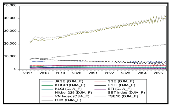 |
|
Graph of an Individual Variable |
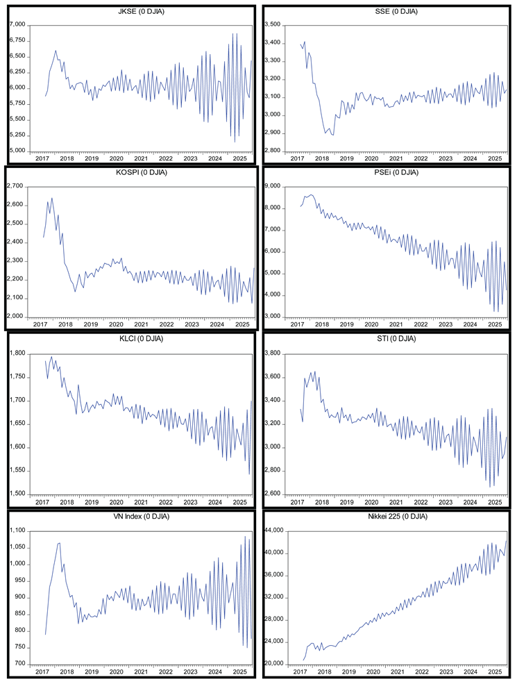 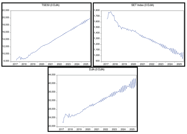
|
References
- Aba, F. X. L. Institutional Change and Macroeconomic Variables in the ASEAN—Indonesia, Vietnam, and Cambodia: The Effects of a Trade War between China and the USA. Economies 2021, 9(4), 195. [Google Scholar] [CrossRef]
- Adrian, T.; Deghi, A.; Qureshi, M. S.; Yenice, M. Y. Trade Policy Uncertainty and Stock Market Tail Risk. Economics Letters 2025, 18–112514. [Google Scholar]
- Aliaga-Miranda, A.; Flores-Vilcapoma, L. R.; Callupe-Cueva, P. C.; Mariños-Alfaro, J. C.; Visurraga-Camargo, L. A.; Chavarry-Becerra, W. S. Cointegration and Economic Adjustment in Agriculture: A VECM Approach to Coffee Price Shocks and Macroeconomic Dynamics. *Economies* 2026, 14(5), 156. [Google Scholar] [CrossRef]
- Amalita, N.; Syafriandi, S.; Kurniawati, Y.; Meilisa, M.; Nafandra, B. Forecasting Macroeconomic Variables in Indonesia Using the Vector Autoregressive Method. ZERO: Journal of Science, Mathematics and Applied Sciences 2026, 10(1), 25–41. [Google Scholar] [CrossRef]
- Antonakakis, N.; Chatziantoniou, I.; Gabauer, D. Refined measures of dynamic connectedness based on time-varying parameter vector autoregressions. Journal of Risk and Financial Management 2020, 13(4), 84. [Google Scholar] [CrossRef]
- Avazkhodjaev, S.; Dhiensiri, N.; Rakhimov, E.; Shayusupova, L.; Turaeva, A. Trade War Shocks and Volatility Spillovers between Fossil Fuel Markets and Biofuel Feedstocks: Empirical Evidence from the US–China Trade Dispute. International Journal of Energy Economics and Policy 2026, 16(1), 719. [Google Scholar]
- Baldwin, R. The Great Trade Hack: How Trump’s Trade War Fails and the World Moves On; CEPR Press, 2025. [Google Scholar]
- Banerjee, A. K.; Sensoy, A.; Goodell, J. W. Volatility connectedness between geopolitical risk and financial markets: Insights from pandemic and military crisis periods. International Review of Economics & Finance 2024, 1–96, 103740. [Google Scholar] [CrossRef]
- Bao, X.; Gao, D.; Wei, Y.; Wu, W.; Zhang, J. Connect to certainty: Domestic trade network and trade policy uncertainty. *Finance Research Letters* 2025, 82, 107639. [Google Scholar] [CrossRef]
- Ben-Ammar, H.; El Abed, R. Economic policy uncertainty and stock market co-movements in BRIC countries: Evidence from wavelet coherence and rolling bootstrap Granger causality. Advances in Decision Sciences 2026, 30(1), 1–32. [Google Scholar] [CrossRef]
- Bonacini, L.; Costa, M.; Pignataro, G. Inequality of Opportunity and Variance Decomposition: A Methodological Insight. Social Indicators Research 2026, 181(3), 72. [Google Scholar] [CrossRef]
- Chen, Y. L.; Yang, J. J.; Chang, Y. T. Stock market volatility spillovers from the US to China: The pivotal role of Hong Kong. Pacific-Basin Finance Journal 2025, 90, 102670. [Google Scholar] [CrossRef]
- Chen, B. X.; Sun, Y. L. Financial market connectedness between the US and China: A new perspective based on non-linear causality networks. Journal of International Financial Markets, Institutions and Money 2024, 1–90, 101886. [Google Scholar] [CrossRef]
- Chen, Y.; Fang, J.; Liu, D. The effects of Trump’s trade war on US financial markets. Journal of International Money and Finance 2023, 1–134, 102842. [Google Scholar] [CrossRef]
- Chimezie, N. G.; Nnenna, A. C.; Ekemma, E. O. B.; Johnmary, A. K. Degree of Shock Elasticity Response to Security Challenges on Investment Growth in Nigeria, 1980 to 2024: A Vector Auto-Regression (VAR) Model Approach. Journal of Terrorism and Defence Studies 2026, 3(1), 68–90. [Google Scholar]
- Chin, M. Y.; Ong, S. L.; Foo, L. P. ASEAN-4–China FDI and Vertical Intra-Industry Trade Links Amid the US–China Trade War—A Spatial Panel Analysis. Sage Open 2026, 16(1), 21582440251410197. [Google Scholar] [CrossRef]
- Dickey, D. A.; Fuller, W. A. Likelihood ratio statistics for autoregressive time series with a unit root. Econometrica: journal of the Econometric Society 1981, 1057–1072. [Google Scholar] [CrossRef]
- Diebold, F. X.; Yilmaz, K. Better to give than to receive: Predictive directional measurement of volatility spillovers. International Journal of Forecasting 2012, 28(1), 57–66. [Google Scholar] [CrossRef]
- Diebold, F. X.; Yılmaz, K. On the network topology of variance decompositions: Measuring the connectedness of financial firms. Journal of Econometrics 2014, 182(1), 119–134. [Google Scholar] [CrossRef]
- Dissanayake, M. B.; Rathnayake, S. S.; Panditharathna, K. M. The Relationship between Macroeconomic Variables, Trading Volume and Stock Returns: Granger Causality Evidence from the Colombo Stock Exchange. Journal of Business and Technology 2026, 10(1). [Google Scholar] [CrossRef]
- Elain, M. I.; Alsabah, M.; Al Saber, A.; Pan, J.; Ali, M.; Boresli, N. Modelling stock yield responses to environmental changes: does geopolitical risk matter? A VECM framework in China. International Journal of Energy Economics and Policy 2026, 16(2), 1083–1096. [Google Scholar] [CrossRef]
- Eissa, M. A.; Al Refai, H. Context-dependent responses to geopolitical risk in Middle Eastern and African stock markets: An asymmetric volatility spillover study. International Review of Economics & Finance 2024, 1–94, 103402. [Google Scholar] [CrossRef]
- El Amine, Y.; Benboubker, M. Assessing the transmission of global market volatility to Moroccan food prices: a VECM-based analysis with forecast error variance decomposition. Journal of Agribusiness in Developing and Emerging Economies 2026, 16(3), 520–541. [Google Scholar]
- Enebeli, E. L.; Enebeli, U. U.; Dakyen, Y. J.; Cherima, Y. J.; Hassan, R. K.; Mikailu, F.; Orya, E. E. A World Bank Data-Driven Analysis of Income, Investment, and Sectoral Change in ECOWAS Economies (2000–2024). Hensard Journal of Policy, Economics and Development 2026, 1(1). [Google Scholar] [CrossRef]
- Faniband, M.; Singh, S. Volatility spillover effects from US and China trade policy uncertainty to the stock market: evidence from an emerging economy. Cogent Economics & Finance 2026, 14(1), 2639204. [Google Scholar] [CrossRef]
- Fishman, E. Chokepoints: American power in the age of economic warfare; Penguin Group, 2025. [Google Scholar]
- Gabauer, D. Volatility impulse response analysis for DCC-GARCH models: The role of volatility transmission mechanisms. Journal of Forecasting 2020, 39(5), 788–796. [Google Scholar] [CrossRef]
- Hamza, A. R.; Shakir, A. H.; Mohsin, R. M. Iraq–China trade and its impact on Iraq’s trade balance and economic growth: An econometric analysis using the ARIMA method. International Journal of Economics and Finance Studies 2025, 17(2), 206–230. [Google Scholar]
- He, F.; Lucey, B.; Wang, Z. Trade policy uncertainty and its impact on the stock market: Evidence from the China–US trade conflict. *Finance Research Letters* 2021, 40, 101753. [Google Scholar] [CrossRef]
- Hoque, M. E.; Soo-Wah, L.; Uddin, M. A.; Rahman, A. Spillover effects of international trade policy uncertainty on the stock market: Evidence from the ‘Fragile Five’ economies. The Journal of International Trade & Economic Development 2023, 32(1), 104–131. [Google Scholar]
- Hu, Z.; Borjigin, S. The amplifying role of geopolitical risks, economic policy uncertainty, and climate risks on energy–stock market volatility spillover across economic cycles. The North American Journal of Economics and Finance 2024, 1–71, 102114. [Google Scholar]
- Hussein, A. N. A. N. Measuring and Analysing the Relationship Between Global Warming and Economic Growth Using the Vector Autoregression (VAR) Model: Iraq as a Case Study for the Period (1990–2016). Academia Open 2026, 11(1), 10–21070. [Google Scholar]
- Idachaba, O.; Iornumbe, S. Foreign Financial Inflows and Unemployment in Nigeria: Evidence from a Time-Series Cointegration Analysis (1987–2024). Impact International Journals and Publications 2026, 2(1), 423–438. [Google Scholar]
- Janmaijaya, M.; Kumar, P. Regional variations in aerosol–temperature coupling over the Indo-Gangetic Plains and Central India: A vector autoregression analysis (2005–2023). The Geographical Journal 2026, 192(1), e70040. [Google Scholar]
- Johansen, S. Estimation and hypothesis testing of cointegration vectors in Gaussian vector autoregressive models. Econometrica: journal of the Econometric Society 1991, 1551–1580. [Google Scholar] [CrossRef]
- Khan, N.; Shah, S. Z. A.; Siddiqui, O. Fluctuations in metals and agricultural commodity markets under US–China trade tensions: evidence from quantile-on-quantile regression and wavelet coherence. The Chinese Economy 2026, 59(2), 173–193. [Google Scholar]
- Kakran, S.; Kumari, V.; Bajaj, P. K.; Sidhu, A. Exploring crisis-driven return spillovers in APEC stock markets: a frequency dynamics analysis. The Journal of Economic Asymmetries 2024, 1–29, e00342. [Google Scholar] [CrossRef]
- Kushwah, S. V. How do Financial Markets Interact? A Vector Error Correction Model (VECM) Analysis of Commodity, Bond, Currency, and Stock Markets. JIMS 8M The Journal of Indian Management and Strategy 2025, 30(2), 34–46. [Google Scholar] [CrossRef]
- Lean, H. H.; Alkhazali, O. M.; Gleason, K.; Yeap, X. W. Connectedness and economic policy uncertainty spillovers to ASEAN stock markets. International Review of Economics & Finance 2024, 90, 167–186. [Google Scholar] [CrossRef]
- Li, R.; Tang, G.; Hong, C.; Li, S.; Li, B.; Xiang, S. A study on economic policy uncertainty, geopolitical risk and stock market spillovers in BRICS countries. The North American Journal of Economics and Finance 2024, 73, 102189. [Google Scholar] [CrossRef]
- Liang, J.; Su, C. Impulse response function-based PINN for dynamic response prediction of engineering structures with nonlinear energy-dissipating devices. Nonlinear Dynamics 2026, 114(2), 143. [Google Scholar] [CrossRef]
- Morales, M. Lag order selection for long-run variance estimation in econometrics. Econometric Reviews 2024, 43(10), 774–795. [Google Scholar] [CrossRef]
- Mukhopadhyay, P.; Parwanee, P. Long-term impacts of environmental and economic growth on GHG emissions, with variations in temperature, rainfall, energy usage, GDP and employment in India: A VECM analysis (1980–2023). In *Sustainable Approaches in Spatial Design*; IGI Global Scientific Publishing, 2026; pp. 93–128. [Google Scholar]
- Nambie, N. B.; Dadzie, P. Trade Realignments, Exchange Rate Volatility, and Financial Stability in Sub-Saharan Africa. Journal of Economics, Finance and Accounting Studies 2026, 8(2), 26–40. [Google Scholar] [CrossRef]
- Nguyen, B. N.; Hoa, P. X.; Luong, H. G.; Nguyen, T. L. A.; Xuan, V. N. Energy transition, economic growth and sustainability in Germany: Evidence from a VECM analysis (2000–2023). Environmental and Sustainability Indicators 2026, 31, 101320. [Google Scholar] [CrossRef]
- Nupap, S.; Htet, T.; Htay, T. T.; Sone, N. P.; Kurubanjerdjit, N. Forecasting Thai Gold Prices Using Correlation-Based Feature Selection and the Vector Error Correction Model (VECM). In 2026, the 18th International Conference on Knowledge and Smart Technology (KST); IEEE, 2026; pp. 497–502. [Google Scholar]
- Nusyirwan, N.; Khairunnisa, K.; Nisa, K.; Misgiyati, M. APPLICATION OF THE PANEL VECTOR AUTOREGRESSIVE (PVAR) MODEL TO THE ANALYSIS OF INFLATION AND GDP RATE. RAGAM: Journal of Statistics & Its Application 2026, 5(1), 19–33. [Google Scholar] [CrossRef]
- Okonkwo, I. V. Macroeconomic Volatility and Economic Growth in Nigeria: An Empirical Analysis of the Fourth Republic (1999–2024). International Journal of Finance, Accounting and Management Studies 2026, 2(5), 109–129. [Google Scholar]
- Özdurak, C. Volatility Spillovers and Interdependencies: The Nexus of Biofuel, Food, and Crude Oil Prices During the COVID-19 Pandemic—A VECM-CCC-GARCH. International Journal of Financial Studies 2026, 14(5), 128. [Google Scholar] [CrossRef]
- Pan, C.; Zhang, W.; Wang, W. Global geopolitical risk and volatility connectedness among China’s sectoral stock markets. *Finance Research Letters* 2023, 1–58, 104487. [Google Scholar] [CrossRef]
- Peng, C.; Deng, H.; Xie, J.; Liu, X. US–China tensions and stock market performance in the US and China: New insights from the time-varying quantile causality method. Finance Research Letters 2025, 1–85, 107888. [Google Scholar] [CrossRef]
- Ritonga, D. A. N.; Syafira, I. N. The impact of exports, imports, real interest rates (RIR) and inflation in Indonesia from 1991 to 2024 using the VECM model. Magisma: Journal of Economics and Business 2026, 14(1), 78–90. [Google Scholar]
- Salachas, E.; Kouretas, G. P.; Laopodis, N. T.; Vlamis, P. Stock market spillovers of global risks and hedging opportunities. European Journal of Political Economy 2024, 1–83, 102533. [Google Scholar] [CrossRef]
- Salem, A. B. M.; Aqel, M. J. Causal Relationship Between AI R&D Investment and Stock Market Performance Using VAR and Granger Causality Models. Journal of Digital Market and Digital Currency 2026, 3(1), 19–37. [Google Scholar] [CrossRef]
- Su, F.; Wang, F.; Xu, Y. Economic policy uncertainty and volatility spillovers among international stock market indices during the COVID-19 outbreak. Asia-Pacific Financial Markets 2025, 32(1), 237–266. [Google Scholar]
- Sultonov, M. Trade-growth dynamics in Central Asia: a causal analysis of international trade and GDP interactions. Journal of Contemporary East Asia Studies 2026, 1–24. [Google Scholar]
- Tabash, M. I.; Sheikh, U. A.; Mensi, W.; Kang, S. H. Quantile-based extended joint connectedness between trade policy uncertainty and GCC Islamic stock sectoral volatility. Borsa Istanbul Review 2024, 24(6), 1146–1165. [Google Scholar] [CrossRef]
- Tran, M. P.-B.; Vo, D. H. Market return spillover from the US to Asia-Pacific countries: The role of geopolitical risk and information and communication technologies. PLOS ONE 2023, 18(12), e0290680. [Google Scholar] [CrossRef] [PubMed]
- Triansyah, F. A.; Karyono, K. National Economic Resilience in the Face of Global Crises: A Policy Analysis Based on IMF and World Bank Reports. Prosperia: Journal of Economic Development, Accounting, and Global Markets 2026, 1(1), 01–09. [Google Scholar]
- Vanegas, A. F. R.; Salinas, P. S.; Arenas, C. D. C. Sectoral and Policy Shocks on Corporate Tax Revenues in Colombia: A VAR Analysis (1995–2023). Revista Finanzas y Política Económica 2026, 18(1), 5. [Google Scholar]
- Xu, Y.; Guan, B.; Lu, W.; Heravi, S. Macroeconomic shocks and volatility spillovers between stock, bond, gold and crude oil markets. *Energy Economics* 2024, 1–136, 107750. [Google Scholar] [CrossRef]
- Yilmazkuday, H. US tariffs and stock prices. *Finance Research Letters* 2025, 1–83, 107708. [Google Scholar] [CrossRef]
- You, K.; Chinthalapati, V. R.; Mishra, T.; Patra, R. International trade networks and stock market connectedness: Evidence from eleven major economies. Journal of International Financial Markets, Institutions and Money 2024, 1–91, 101939. [Google Scholar] [CrossRef]
- Zeng, W.; Johnson, W.; Rudin-Rush, L. United States and Global Macroeconomic Projections from 2024 to 2034. 2025. [Google Scholar] [CrossRef] [PubMed]
- Zhang, Y.; He, J.; He, M.; Li, S. Geopolitical risk and stock market volatility: A global perspective. Finance Research Letters 2023, 1–53, 103620. [Google Scholar] [CrossRef]
- Zhao, M.; Park, H. Research on the dynamic interrelationship between economic policy uncertainty and stock market returns. Journal of Risk and Financial Management 2024, 11–17(8), 347. [Google Scholar]
Figure 1.
Movements in Asian and US Stock Indices, January 2017–December 2024. Source: Data processing and analysis by the researcher.
Figure 1.
Movements in Asian and US Stock Indices, January 2017–December 2024. Source: Data processing and analysis by the researcher.
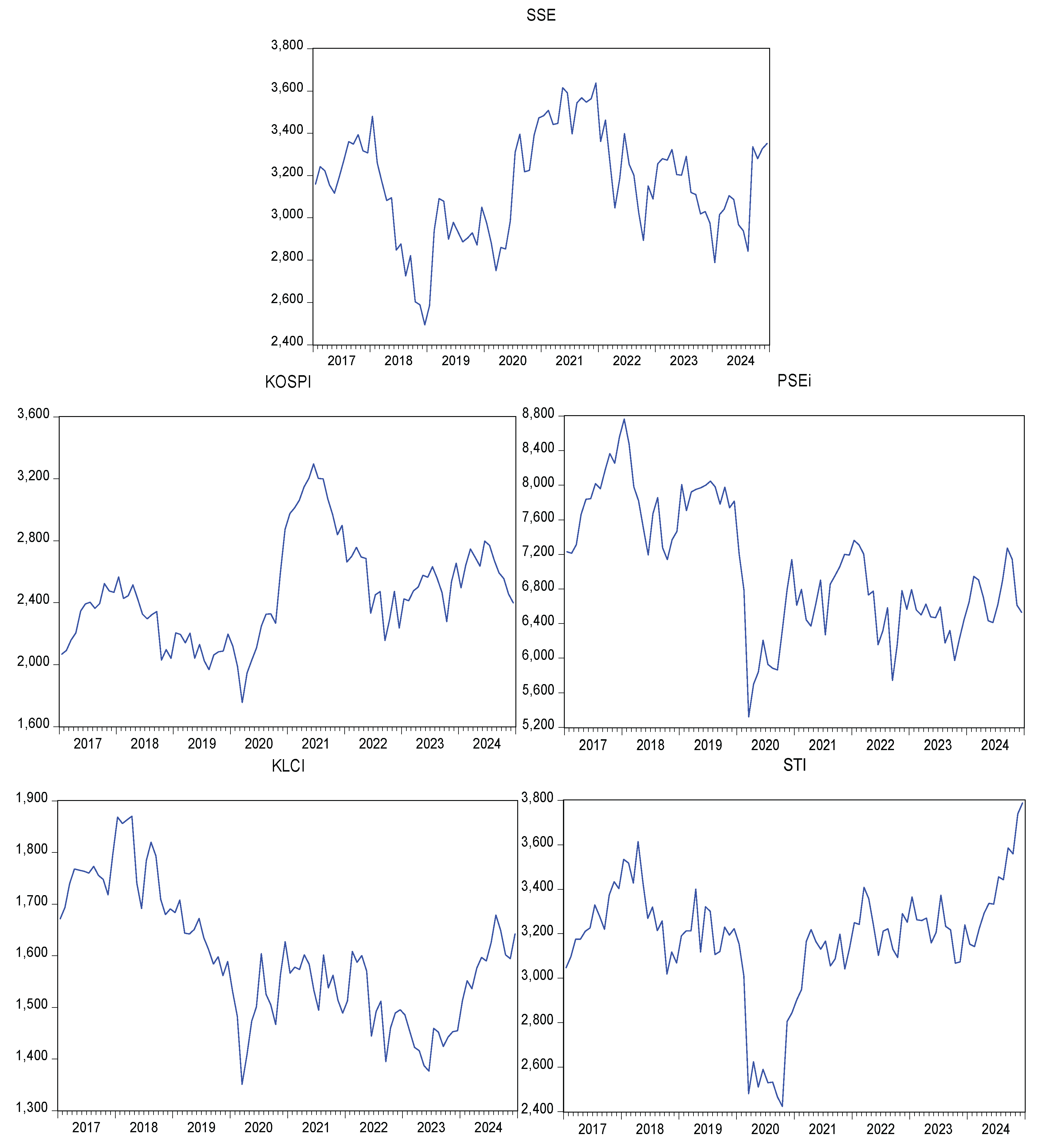
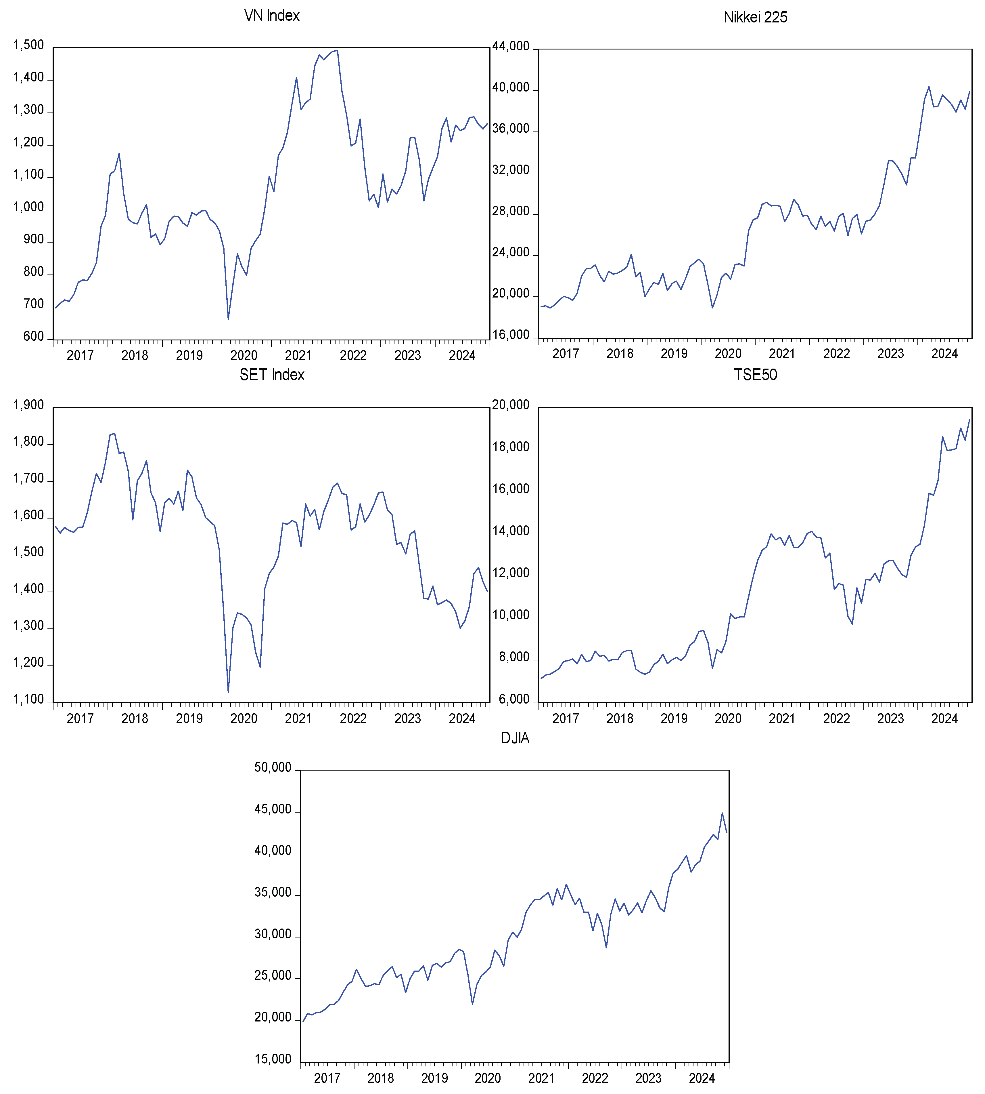
Figure 2.
Impulse Response Function (IRF) Monthly Stock Market Indices for Asia and the United States, January 2017–December 2024. Source: Data processing and analysis by the researcher.
Figure 2.
Impulse Response Function (IRF) Monthly Stock Market Indices for Asia and the United States, January 2017–December 2024. Source: Data processing and analysis by the researcher.
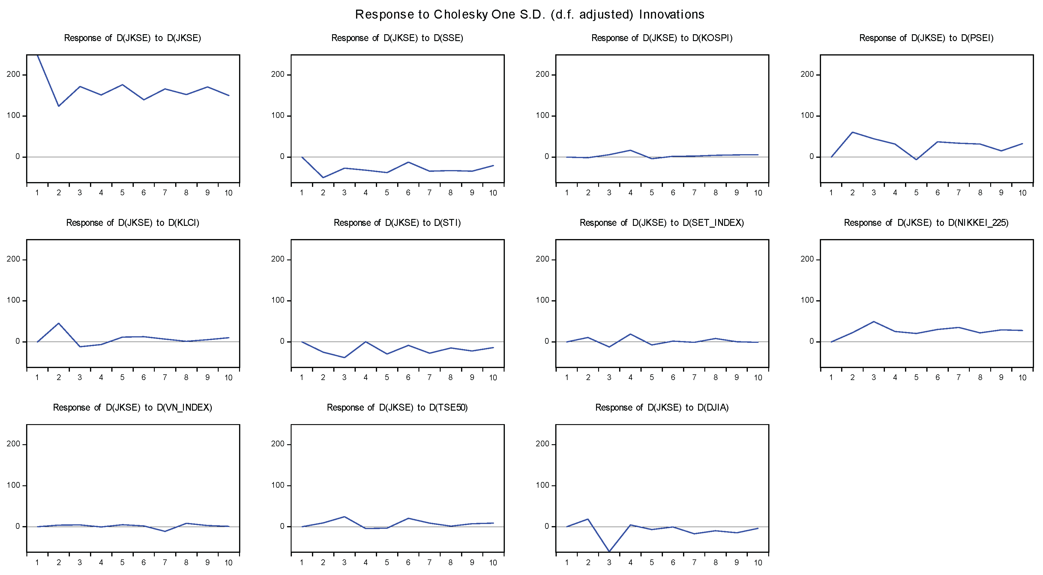
Figure 3.
VECM Model Forecast for Monthly Stock Indices in Asia and the United States, January 2017 – December 2024. Source: Data processing and analysis by the researcher.
Figure 3.
VECM Model Forecast for Monthly Stock Indices in Asia and the United States, January 2017 – December 2024. Source: Data processing and analysis by the researcher.
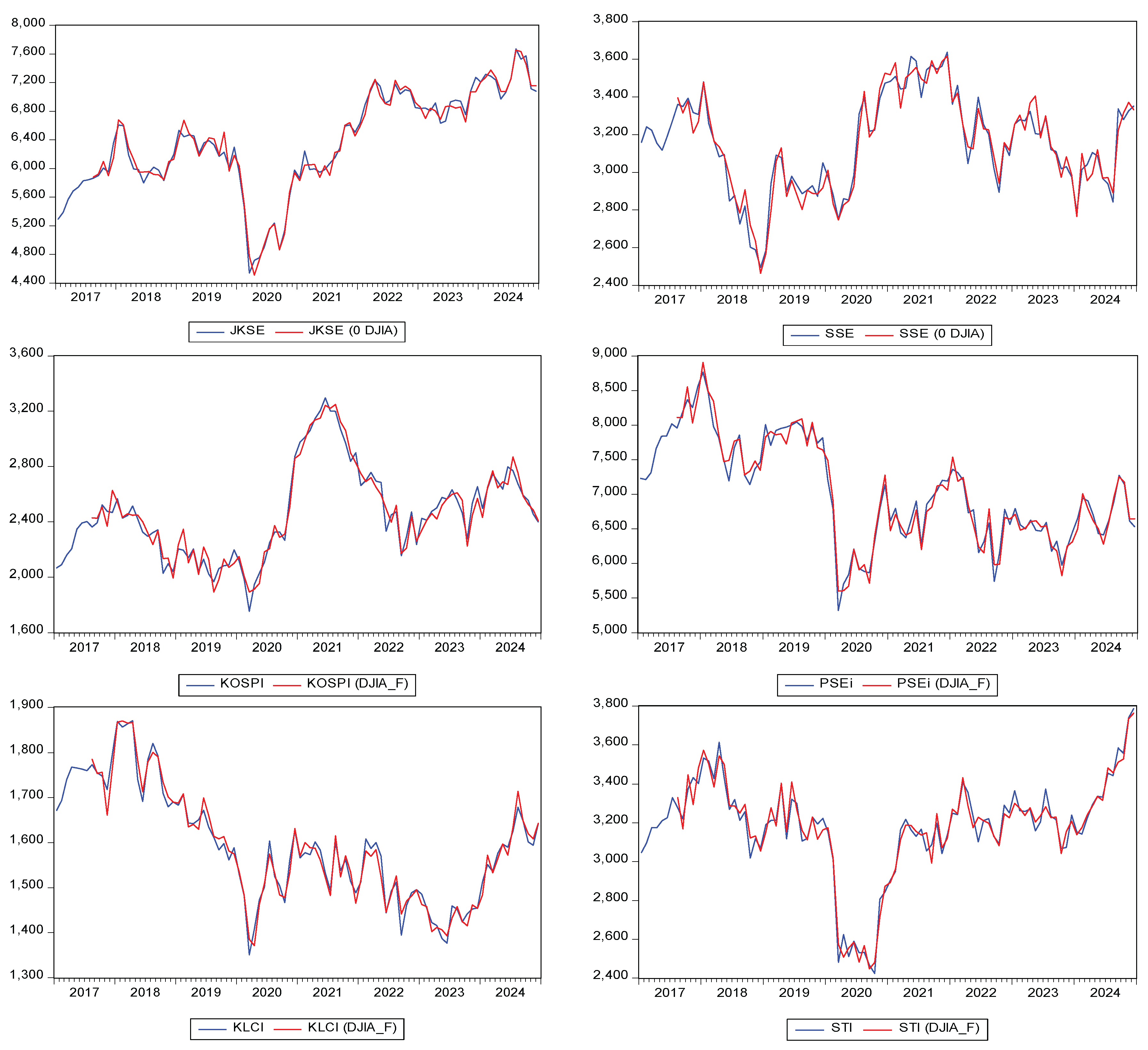
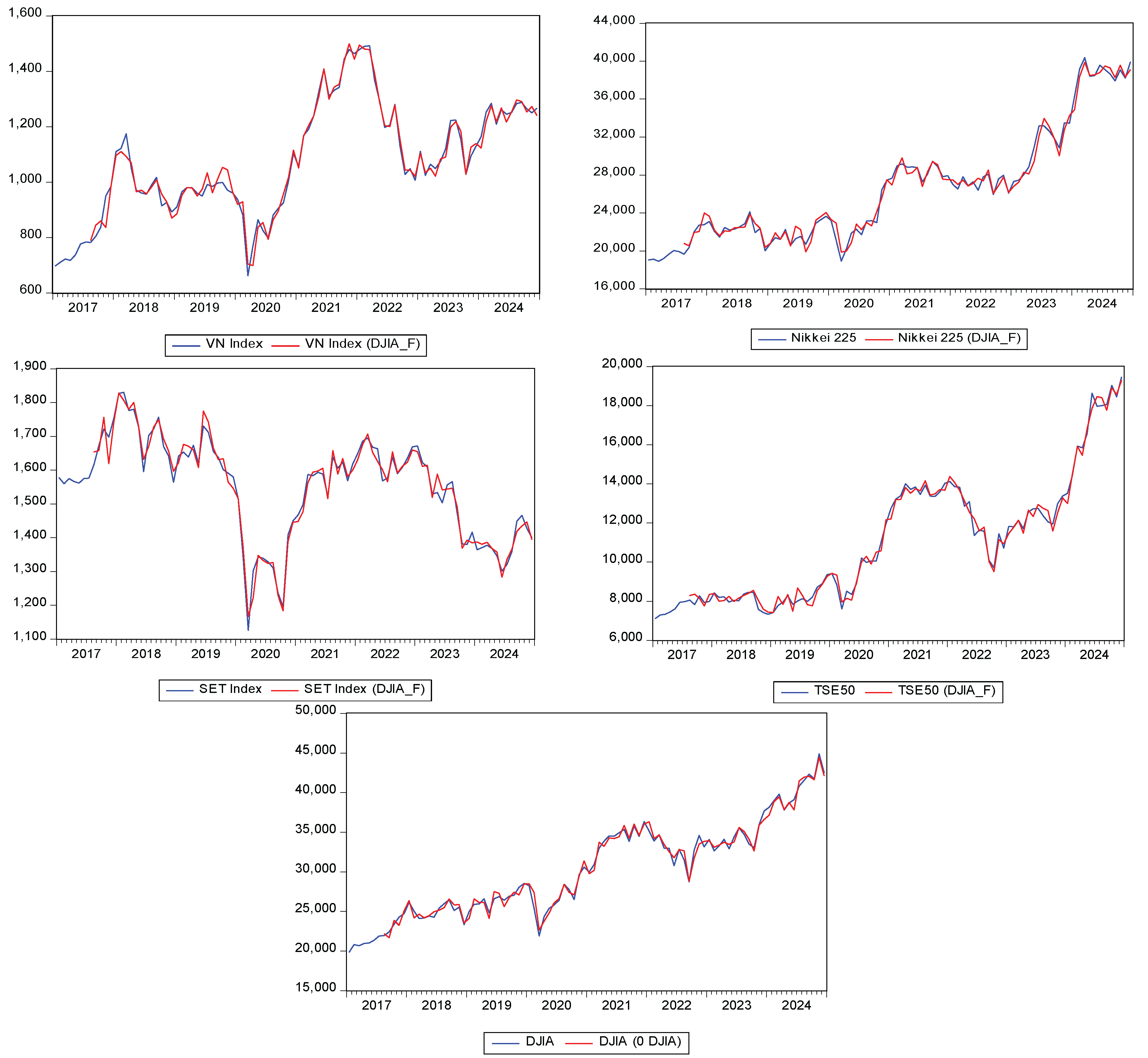

Table 1.
Stationarity Tests of the Monthly Stock Market Index and the United States, January 2017–December 2024.
Table 1.
Stationarity Tests of the Monthly Stock Market Index and the United States, January 2017–December 2024.
| Stock Index | Unit Root Test | |||||
| Level | First Difference | |||||
| t-Statistic |
Calculated t-value (5% Significance Level) |
Prob.* | t-Statistic |
t-value (5% significance level) |
Prob.* | |
| Indonesia (^JKSE) | -1.728439 | -2.892200 | 0.4138 | -8.402967 | -2.892536 | 0.0000 |
| China (^SSE) | -2.585910 | 0.0994 | -10.51872 | 0.0000 | ||
| South Korea (^KOSPI) | -2.062285 | 0.2604 | -10.28708 | 0.0000 | ||
| Philippines (^PSEi) | -2.185886 | 0.2128 | -9.998390 | 0.0000 | ||
| Malaysia (^KLCI) | -1.986762 | 0.2922 | -9.825738 | 0.0000 | ||
| Singapore (^STI) | -1.836967 | 0.3607 | -11.68863 | 0.0001 | ||
| Vietnam (^VN Index) | -1.943078 | 0.3115 | -8.895285 | 0.0000 | ||
| Japan (^Nikkei 225) | -0.037413 | 0.9521 | -9.602110 | 0.0000 | ||
| Thailand (^SET Index) | -1.978738 | 0.2957 | -9.226301 | 0.0000 | ||
| Taiwan (^TSE50) | 0.545718 | 0.9875 | -10.31524 | 0.0000 | ||
| USA (^DJIA) | -0.861616 | 0.7963 | -11.35663 | 0.0001 | ||
Source: Data processing and analysis by the researcher.
Table 2.
Testing the Optimum Lag for the Monthly Stock Market Index in Asia and the United States, January 2017–December 2024.
Table 2.
Testing the Optimum Lag for the Monthly Stock Market Index in Asia and the United States, January 2017–December 2024.
| VAR Lag Order Selection Criteria | ||||||
| Endogenous variables: D(JKSE) D(SSE) D(KOSPI) D(PSEI) D(KLCI) D(STI) D(VN_INDEX) D(NIKKEI_225) D(SET_INDEX) D(TSE50) D(DJIA) | ||||||
| Exogenous variables: C | ||||||
| Date: 23/05/25 Time: 09:11 | ||||||
| Sample: January 2017 – December 2024 | ||||||
| Included observations: 89 | ||||||
| Lag | LogL | LR | FPE | AIC | SC | HQ |
| 0 | -6372.703 | NA | 5.55e+48* | 143.4540 | 143.7616* | 143.5780* |
| 1 | -6287.826 | 146.8654 | 1.27e+49 | 144.2658 | 147.9568 | 145.7535 |
| 2 | -6200.571 | 129.4115 | 3.04e+49 | 145.0241 | 152.0985 | 147.8756 |
| 3 | -6119.023 | 100.7901 | 1.01e+50 | 145.9106 | 156.3685 | 150.1259 |
| 4 | -5949.989 | 167.1351* | 6.78e+49 | 144.8312 | 158.6725 | 150.4102 |
| 5 | -5804.318 | 108.0256 | 1.45e+50 | 144.2768 | 161.5015 | 151.2196 |
| 6 | -5511.371 | 144.8279 | 3.88e+49 | 140.4128* | 161.0210 | 148.7194 |
| * indicates the lag order selected by the criterion | ||||||
| LR: sequential modified LR test statistic (each test at the 5% significance level) | ||||||
| FPE: Final prediction error | ||||||
| AIC: Akaike information criterion | ||||||
| SC: Schwarz information criterion | ||||||
| HQ: Hannan–Quinn information criterion | ||||||
Source: Results of data processing and analysis by the researcher.
Table 3.
Testing the Stability of Monthly Stock Market Indices in Asia and the United States, January 2017–December 2024.
Table 3.
Testing the Stability of Monthly Stock Market Indices in Asia and the United States, January 2017–December 2024.
| Roots of the Characteristic Polynomial Endogenous variables: D(JKSE) D(SSE) D(KOSPI) D(PSEI) D(KLCI) D(STI) D(VN_INDEX) D(NIKKEI_225) D(SET_INDEX) D(TSE50) D(DJIA) | |
| Exogenous variables: C | |
| Lag specification: 1 2 | |
| Date: 23/05/25 Time: 11:12 | |
| Root | Modulus |
| -0.305621 + 0.585892i | 0.660813 |
| -0.305621 - 0.585892i | 0.660813 |
| -0.104329 + 0.652212i | 0.660504 |
| -0.104329 - 0.652212i | 0.660504 |
| -0.658700 | 0.658700 |
| 0.298278 - 0.503200i | 0.584962 |
| 0.298278 + 0.503200i | 0.584962 |
| 0.377501 – 0.435362i | 0.576235 |
| 0.377501 + 0.435362i | 0.576235 |
| -0.524874 + 0.214546i | 0.567029 |
| -0.524874 - 0.214546i | 0.567029 |
| -0.537729 - 0.131610i | 0.553601 |
| -0.537729 + 0.131610i | 0.553601 |
| 0.553476 | 0.553476 |
| -0.182742 - 0.473317i | 0.507369 |
| -0.182742 + 0.473317i | 0.507369 |
| 0.007249 + 0.462929i | 0.462986 |
| 0.007249 - 0.462929i | 0.462986 |
| 0.430047 | 0.430047 |
| 0.389589 + 0.127887i | 0.410042 |
| 0.389589 – 0.127887i | 0.410042 |
| 0.142878 | 0.142878 |
| No root lies outside the unit circle. | |
| VAR satisfies the stability condition. Source: Results of data processing and analysis by the researcher | |
Table 4.
Testing the Causality of Monthly Stock Market Indices in Asia and the United States, January 2017–December 2024.
Table 4.
Testing the Causality of Monthly Stock Market Indices in Asia and the United States, January 2017–December 2024.
| No. | Null Hypothesis | Prob. | H0 | Causal Relationship |
| 1 | STI does not Granger-cause JKSE | 0.3936 | Accept | None |
| JKSE does not Granger-cause STI | 0.0205 | Reject | Yes | |
| 2 | PSEI does not Granger-cause SSE | 0.0108 | Reject | Yes |
| SSE does not Granger-cause PSEI | 0.5092 | Accept | None | |
| 3 | STI does not Granger-cause SSE | 0.0260 | Reject | Yes |
| SSE does not Granger-cause STI | 0.6349 | Accept | None | |
| 4 | NIKKEI_225 does not Granger-cause SSE | 0.0234 | Reject | Yes |
| SSE does not Granger-cause NIKKEI_225 | 0.2860 | Accept | None | |
| 5 | The DJIA does not Granger-cause the SSE | 0.4901 | Accept | None |
| The SSE does not Granger-cause the DJIA | 0.0194 | Reject | Yes | |
| 6 | The STI does not Granger-cause the KOSPI | 0.0091 | Reject | Yes |
| KOSPI does not Granger-cause STI | 0.6974 | Accept | None | |
| 7 | VN_INDEX does not Granger-cause KOSPI | 0.7941 | Accept | None |
| KOSPI does not Granger-cause VN_INDEX | 0.0101 | Reject | There are | |
| 8 | KLCI does not Granger-cause PSEI | 0.0064 | Reject | Yes |
| PSEI does not Granger-cause KLCI | 0.3744 | Accept | None | |
| 9 | SET_INDEX does not Granger-cause KLCI | 0.1678 | Accept | None |
| KLCI does not Granger-cause SET_INDEX | 0.0091 | Reject | Yes | |
| 10 | TSE50 does not Granger-cause SET_INDEX | 0.4355 | Accept | None |
| SET_INDEX does not Granger-cause TSE50 | 0.0044 | Reject | Yes |
Source: Results of data processing and analysis by the researcher.
Table 5.
Cointegration Test of Monthly Stock Market Indices in Asia and the United States, January 2017–December 2024.
Table 5.
Cointegration Test of Monthly Stock Market Indices in Asia and the United States, January 2017–December 2024.
|
Unrestricted Cointegration Rank Test (Trace) |
Unrestricted Cointegration Rank Test (Maximum Eigenvalue) |
||||||
| Hypothesised No. of CE(s) |
Trace Statistic |
0.05 Critical Value |
Prob.** | Hypothesised No. of CE(s) |
Max-Eigen Statistic |
0.05 Critical Value |
Prob.** |
| None * | 567.0576 | 298.1594 | 0.0000 | None * | 150.0052 | 71.33542 | 0.0000 |
| At most 1 * | 417.0524 | 251.2650 | 0.0000 | At most 1 * | 113.7848 | 65.30016 | 0.0000 |
| At most 2 * | 303.2675 | 208.4374 | 0.0000 | At most 2 * | 82.41771 | 59.24000 | 0.0001 |
| At most 3 * | 220.8498 | 169.5991 | 0.0000 | At most 3 * | 58.50773 | 53.18784 | 0.0131 |
| At most 4 * | 162.3421 | 134.6780 | 0.0004 | At most 4 | 46.85994 | 47.07897 | 0.0527 |
| At most 5 * | 115.4822 | 103.8473 | 0.0068 | At most 5 * | 46.37637 | 40.95680 | 0.0112 |
| At most 6 | 69.10580 | 76.97277 | 0.1711 | At most 6 | 23.35172 | 34.80587 | 0.5712 |
| At most 7 | 45.75408 | 54.07904 | 0.2231 | At most 7 | 20.14451 | 28.58808 | 0.4012 |
| At most 8 | 25.60957 | 35.19275 | 0.3641 | At most 8 | 12.95301 | 22.29962 | 0.5613 |
| At most 9 | 12.65656 | 20.26184 | 0.3918 | At most 9 | 8.473569 | 15.89210 | 0.4923 |
| At most 10 | 4.182990 | 9.164546 | 0.3855 | At most 10 | 4.182990 | 9.164546 | 0.3855 |
Source: Results of data processing and analysis by the researcher.
Table 6.
VECM Estimates (Long-Run Relationships) for Monthly Indices Asian and US Stock Markets, January 2017–December 2024.
Table 6.
VECM Estimates (Long-Run Relationships) for Monthly Indices Asian and US Stock Markets, January 2017–December 2024.
| Long-Run Relationships | |||||||
| CointEq: | CointEq1 | CointEq: | CointEq1 | CointEq: | CointEq1 | CointEq: | CointEq1 |
| D(JKSE(-1)) | 1.000000 | D(SSE(-1)) | 1.000000 | D(KOSPI(-1)) | 1.000000 | D(PSEI(-1)) | 1.000000 |
| D(KLCI(-1)) | 4.837238 | D(STI(-1)) | -6.689122 | D(STI(-1)) | 8.133839 | D(KLCI(-1)) | -6.301639 |
| (2.31595) | (1.19762) | (1.44468) | (3.07477) | ||||
| [ 2.08866] | [-5.58537] | [ 5.63021] | [-2.04947] | ||||
| D(STI(-1)) | 8.091343 | D(SET_INDEX(-1)) | 15.92922 | D(SET_INDEX(-1)) | -19.36962 | D(STI(-1)) | -10.54087 |
| (1.35641) | (1.79095) | (2.18120) | (1.80978) | ||||
| [ 5.96527] | [ 8.89426] | [-8.88025] | [-5.82441] | ||||
| D(SET_INDEX(-1)) | -19.26842 | D(NIKKEI_225(-1)) | 0.566292 | D(NIKKEI_225(-1)) | -0.688600 | D(SET_INDEX(-1)) | 25.10164 |
| (2.17870) | (0.07874) | (0.08589) | (2.82094) | ||||
| [-8.84400] | [ 7.19187] | [-8.01721] | [ 8.89831] | ||||
| D(NIKKEI_225(-1)) | -0.685003 | D(VN_INDEX(-1)) | -4.430276 | D(VN_INDEX(-1)) | 5.387128 | D(NIKKEI_225(-1)) | 0.892377 |
| (0.10040) | (1.18092) | (1.39693) | (0.13333) | ||||
| [-6.82298] | [-3.75154] | [ 3.85640] | [ 6.69277] | ||||
| D(VN_INDEX(-1)) | 5.358982 | D(VN_INDEX(-1)) | -6.981333 | ||||
| (1.31574) | CointEq: | CointEq1 | CointEq: | CointEq1 | (1.86334) | ||
| [ 4.07298] | D(STI(-1)) | 1.000000 | D(VN_INDEX(-1)) | 1.000000 | [-3.74667] | ||
| D(TSE50(-1)) | -0.406717 | D(SET_INDEX(-1)) | -2.381362 | D(STI(-1)) | 1.509866 | ||
| (0.18692) | (0.21572) | (0.26236) | CointEq: | CointEq1 | |||
| [-2.17586] | [-11.0390] | [ 5.75500] | D(NIKKEI_225(-1)) | 1.000000 | |||
| D(NIKKEI_225(-1)) | -0.084659 | D(NIKKEI_225(-1)) | -0.127823 | D(STI(-1)) | -11.81214 | ||
| CointEq: | CointEq1 | (0.01262) | (0.01877) | (2.11528) | |||
| D(KLCI(-1)) | 1.000000 | [-6.70585] | [-6.80823] | [-5.58419] | |||
| D(STI(-1)) | 1.672720 | D(VN_INDEX(-1)) | 0.662311 | D(SET_INDEX(-1)) | -3.595537 | D(VN_INDEX(-1)) | -7.823302 |
| (0.29999) | (0.17112) | (0.39895) | (2.05181) | ||||
| [ 5.57587] | [ 3.87041] | [-9.01246] | [-3.81287] | ||||
| D(SET_INDEX(-1)) | -3.983351 | D(TSE50(-1)) | -0.050266 | D(TSE50(-1)) | -0.075894 | D(SET_INDEX(-1)) | 28.12898 |
| (0.44757) | (0.02166) | (0.03603) | (3.10361) | ||||
| [-8.89996] | [-2.32093] | [-2.10630] | [ 9.06332] | ||||
| D(NIKKEI_225(-1)) | -0.141610 | ||||||
| (0.02093) | CointEq: | CointEq1 | CointEq: | CointEq1 | CointEq: | CointEq1 | |
| [-6.76601] | D(SET_INDEX(-1)) | 1.000000 | D(TSE50(-1)) | 1.000000 | D(DJIA(-1)) | 1.000000 | |
| D(VN_INDEX(-1)) | 1.107860 | D(STI(-1)) | -0.419928 | D(KLCI(-1)) | -11.89339 | D(STI(-1)) | 34.66139 |
| (0.29574) | (0.06041) | (5.67142) | (6.09270) | ||||
| [ 3.74610] | [-6.95173] | [-2.09708] | [ 5.68900] | ||||
| D(TSE50(-1)) | -0.084080 | D(VN_INDEX(-1)) | -0.278123 | D(STI(-1)) | -19.89431 | D(VN_INDEX(-1)) | 22.95661 |
| (0.04057) | (0.07286) | (3.04789) | (6.11307) | ||||
| [-2.07256] | [-3.81698] | [-6.52723] | [ 3.75533] | ||||
| D(NIKKEI_225(-1)) | 0.035551 | D(VN_INDEX(-1)) | -13.17621 | D(NIKKEI_225(-1)) | -2.934388 | ||
| (0.00519) | (3.30743) | (0.43674) | |||||
| [ 6.85403] | [-3.98382] | [-6.71884] | |||||
| D(TSE50(-1)) | 0.021108 | D(NIKKEI_225(-1)) | 1.684226 | D(SET_INDEX(-1)) | -82.54134 | ||
| (0.00885) | (0.24760) | (8.53521) | |||||
| [ 2.38530] | [ 6.80213] | [-9.67069] | |||||
| D(SET_INDEX(-1)) | 47.37555 | D(TSE50(-1)) | -1.742277 | ||||
| (4.44742) | (0.78465) | ||||||
| [ 10.6524] | [-2.22044] | ||||||
Source: Results of data processing and analysis by the researcher.
Table 7.
VECM Estimates (Short-Run Relationships) for Monthly Indices Asian and US Stock Market Indices, January 2017 – December 2024.
Table 7.
VECM Estimates (Short-Run Relationships) for Monthly Indices Asian and US Stock Market Indices, January 2017 – December 2024.
| Short-Run Relationship | |||||
| JKSE Dependent | KOSPI Dependent | ||||
| Stock Index | Coefficient | t-statistic | Stock Index | Coefficient | t-statistic |
| D(JKSE(-1),2) – D(JKSE,2) | -0.824091 | [-3.83980] | D(KOSPI(-1),2) - D(KOSPI,2) | -0.956130 | [-3.02479] |
| D(JKSE(-3),2) - D(JKSE,2) | -0.547240 | [-2.06774] | D(DJIA(-5),2) - D(KOSPI,2) | 0.078427 | [ 2.15628] |
| D(SSE(-1),2) - D(JKSE,2) | -1.128565 | [-3.12094] | PSEi Dependent | ||
| D(KOSPI(-4),2) – D(JKSE,2) | 1.297821 | [ 2.14877] | D(JKSE(-4),2) - D(PSEi,2) | 0.981442 | [ 2.43847] |
| D(PSEI(-1),2) – D(JKSE,2) | 0.506049 | [ 2.38004] | D(SSE(-1),2) – D(PSEI,2) | -1.933574 | [-3.95294] |
| D(STI(-1),2) – D(JKSE,2) | 1.833011 | [ 2.51423] | D(SSE(-4),2) – D(PSEI,2) | -0.961927 | [-2.07163] |
| D(STI(-5),2) – D(JKSE,2) | -1.273249 | [-2.54893] | D(KOSPI(-1),2) - D(PSEI,2) | -1.553881 | [-2.24633] |
| D(SET_INDEX(-1),2) - D(JKSE,2) | -3.687332 | [-2.17530 | D(STI(-5),2) - D(PSEI,2) | -2.021232 | [-2.99130] |
| D(NIKKEI_225(-1),2) - D(JKSE,2) | -0.173297 | [-2.54038] | D(NIKKEI_225(-2),2) - D(PSEI,2) | -0.190502 | [-2.54458] |
| D(NIKKEI_225(-2),2) - D(JKSE,2) | -0.123126 | [-2.22467] | D(NIKKEI_225(-3),2) - D(PSEI,2) | -0.133648 | [-2.09495] |
| D(NIKKEI_225(-3),2) - D(JKSE,2) | -0.107667 | [-2.28293] | D(NIKKEI_225(-5),2) - D(PSEI,2) | -0.320507 | [-4.41360] |
| D(NIKKEI_225(-4),2) - D(JKSE,2) | -0.135578 | [-3.00353] | D(DJIA(-1),2) - D(PSEI,2) | 0.115687 | [ 2.13622] |
| D(NIKKEI_225(-5),2) - D(JKSE,2) | -0.167563 | [-3.12129] | D(DJIA(-5),2) - D(PSEI,2) | 0.217034 | [ 2.72674] |
| SSE Dependent | NIKKEI 225 Dependency | ||||
| D(JKSE(-4),2) - D(SSE,2) | 0.425739 | [ 2.34410] | D(JKSE(-4),2) - D(NIKKEI_225,2) | 5.434149 | [ 2.86912] |
| D(SSE(-1),2) - D(SSE,2) | -0.960117 | [-4.34973] | D(KLCI(-3),2) - D(NIKKEI_225,2) | -16.94097 | [-2.20742] |
| D(SSE(-3),2) - D(SSE,2) | -0.418032 | [-2.29522] | D(STI(-5),2) - D(NIKKEI_225,2) | -6.695764 | [-2.10576] |
| D(SSE(-4),2) - D(SSE,2) | -0.601685 | [-2.87157] | D(DJIA(-5),2) - D(NIKKEI_225,2) | 0.947797 | [ 2.53044] |
| D(DJIA(-3),2) - D(SSE,2) | -0.068678 | [-2.06054] | STI Dependent | ||
| KLCI Dependent | D(JKSE(-4),2) - D(STI,2) | 0.578794 | [ 3.82012] | ||
| D(JKSE(-4),2) - D(KLCI,2) | 0.157982 | [ 2.79787] | D(JKSE(-5),2) – D(STI,2) | 0.302631 | [ 2.55748] |
| D(SSE(-1),2) – D(KLCI,2) | -0.416988 | [-6.07645] | D(SSE(-1),2) – D(STI,2) | -0.695912 | [-3.77931] |
| D(SSE(-2),2) – D(KLCI,2) | -0.138295 | [-2.22253] | D(KOSPI(-3),2) - D(STI,2) | 0.713352 | [ 2.27237] |
| D(SSE(-3),2) - D(KLCI,2) | -0.155916 | [-2.75355] | D(KLCI(-3),2) – D(STI,2) | -1.803739 | [-2.93802] |
| D(SSE(-4),2) – D(KLCI,2) | -0.230535 | [-3.53895] | D(PSEI(-1),2) – D(STI,2) | 0.308793 | [ 2.85206] |
| D(KOSPI(-1),2) - D(KLCI,2) | -0.372849 | [-3.84198] | D(PSEI(-2),2) - D(STI,2) | 0.293849 | [ 2.44465] |
| D(KOSPI(-3),2) - D(KLCI,2) | 0.355283 | [ 3.03681] | D(PSEI(-5),2) – D(STI,2) | -0.164059 | [-2.13855] |
| D(KOSPI(-4),2) - D(KLCI,2) | 0.392750 | [ 3.42656] | D(STI(-1),2) - D(STI,2) | -0.959417 | [-2.58433] |
| D(KOSPI(-5),2) - D(KLCI,2) | 0.333940 | [ 3.33137] | D(STI(-2),2) - D(STI,2) | -1.053010 | [-2.84015] |
| D(KLCI(-1),2) – D(KLCI,2) | -0.995492 | [-5.16383] | D(STI(-5),2) - D(STI,2) | -0.869953 | [-3.42011] |
| D(KLCI(-2),2) - D(KLCI,2) | -0.958121 | [-4.35968] | D(NIKKEI_225(-1),2) - D(STI,2) | -0.082683 | [-2.38025] |
| D(KLCI(-3),2) - D(KLCI,2) | -1.039874 | [-4.54495] | D(NIKKEI_225(-5),2) - D(STI,2) | -0.085525 | [-3.12860] |
| D(KLCI(-4),2) - D(KLCI,2) | -0.783646 | [-3.65148] | D(DJIA(-2),2) - D(STI,2) | -0.068141 | [-2.71265] |
| D(KLCI(-5),2) - D(KLCI,2) | -0.494214 | [-2.90318] | D(DJIA(-3),2) - D(STI,2) | -0.065887 | [-2.36964] |
| D(PSEI(-1),2) - D(KLCI,2) | 0.155143 | [ 3.84495] | D(DJIA(-4),2) – D(STI,2) | -0.070307 | [-2.29205] |
| D(PSEI(-2),2) - D(KLCI,2) | 0.094695 | [ 2.11391] | SET INDEX Dependent | ||
| D(STI(-2),2) - D(KLCI,2) | -0.391125 | [-2.83068] | D(JKSE(-2),2) - D(SET_INDEX,2) | -0.210676 | [-3.25337] |
| D(STI(-4),2) - D(KLCI,2) | -0.249633 | [-2.39135] | D(SSE(-1),2) - D(SET_INDEX,2) | -0.261640 | [-2.90836] |
| D(STI(-5),2) - D(KLCI,2) | -0.404009 | [-4.26189] | D(SSE(-3),2) - D(SET_INDEX,2) | -0.236922 | [-3.19172] |
| D(SET_INDEX(-2),2) - D(KLCI,2) | 0.708112 | [ 2.31643] | D(SSE(-5),2) - D(SET_INDEX,2) | -0.148185 | [-2.08885] |
| D(SET_INDEX(-3),2) - D(KLCI,2) | 0.677946 | [ 2.50283] | D(KOSPI(-1),2) - D(SET_INDEX,2) | -0.297644 | [-2.33957] |
| D(NIKKEI_225(-2),2) - D(KLCI,2) | -0.021615 | [-2.05798] | D(KOSPI(-5),2) - D(SET_INDEX,2) | 0.466342 | [ 3.54876] |
| D(NIKKEI_225(-5),2) - D(KLCI,2) | -0.040201 | [-3.94600] | D(KLCI(-2),2) - D(SET_INDEX,2) | -0.635803 | [-2.20686] |
| D(VN_INDEX(-3),2) - D(KLCI,2) | 0.426502 | [ 3.12539] | D(KLCI(-3),2) - D(SET_INDEX,2) | -0.724920 | [-2.41689] |
| D(TSE50(-1),2) – D(KLCI,2) | 0.073965 | [ 3.74810] | D(KLCI(-5),2) - D(SET_INDEX,2) | -0.843582 | [-3.78011] |
| D(TSE50(-2),2) - D(KLCI,2) | 0.087831 | [ 3.87171] | D(PSEI(-1),2) – D(SET_INDEX,2) | 0.160344 | [ 3.03130] |
| D(DJIA(-2),2) - D(KLCI,2) | -0.022249 | [-2.37665] | D(PSEI(-2),2) - D(SET_INDEX,2) | 0.220993 | [ 3.76319] |
| D(DJIA(-3),2) - D(KLCI,2) | -0.028679 | [-2.76766] | D(STI(-1),2) - D(SET_INDEX,2) | -0.414000 | [-2.28258] |
| D(DJIA(-5),2) - D(KLCI,2) | 0.043499 | [ 3.89552] | D(STI(-2),2) - D(SET_INDEX,2) | -0.474228 | [-2.61807] |
| VN INDEX Dependent | D(STI(-4),2) - D(SET_INDEX,2) | -0.287325 | [-2.09959] | ||
| D(JKSE(-4),2) - D(VN_INDEX,2) | 0.199565 | [ 2.38379] | D(STI(-5),2) - D(SET_INDEX,2) | -0.298474 | [-2.40179] |
| D(STI(-1),2) - D(VN_INDEX,2) | 0.448668 | [ 2.18724] | D(NIKKEI_225(-5),2) - D(SET_INDEX,2) | -0.033921 | [-2.53984] |
| D(STI(-3),2) - D(VN_INDEX,2) | 0.384202 | [ 2.18673] | D(DJIA(-3),2) - D(SET_INDEX,2) | -0.039108 | [-2.87898] |
| D(SET_INDEX(-1),2) - D(VN_INDEX,2) | -1.038070 | [-2.17653] | D(DJIA(-4),2) - D(SET_INDEX,2) | -0.043605 | [-2.90972] |
| D(SET_INDEX(-2),2) - D(VN_INDEX,2) | -1.046233 | [-2.30840] | TSE 50 | ||
| D(NIKKEI_225(-1),2) - D(VN_INDEX,2) | -0.046930 | [-2.44508] | D(JKSE(-1),2) - D(TSE50,2) | -1.231863 | [-2.05267] |
| D(NIKKEI_225(-2),2) - D(VN_INDEX,2) | -0.033466 | [-2.14911] | D(SSE(-1),2) - D(TSE50,2) | -2.201188 | [-2.17690] |
| D(NIKKEI_225(-3),2) - D(VN_INDEX,2) | -0.027935 | [-2.10522] | D(PSEI(-1),2) - D(TSE50,2) | 1.980481 | [ 3.33108] |
| D(NIKKEI_225(-5),2) - D(VN_INDEX,2) | -0.048470 | [-3.20890] | D(PSEI(-2),2) - D(TSE50,2) | 1.936560 | [ 2.93390] |
| D(VN_INDEX(-1),2) - D(VN_INDEX,2) | -0.444328 | [-2.33328] | D(PSEI(-3),2) - D(TSE50,2) | 1.600249 | [ 2.23327] |
| D(VN_INDEX(-2),2) - D(VN_INDEX,2) | -0.447132 | [-2.29063] | D(TSE50(-1),2) - D(TSE50,2) | -0.613867 | [-2.11114] |
| D(DJIA(-1),2) - D(VN_INDEX,2) | 0.032368 | [ 2.87343] | D(DJIA(-3),2) - D(TSE50,2) | -0.491681 | [-3.22025] |
| D(DJIA(-5),2) - D(VN_INDEX,2) | 0.039534 | [ 2.38790] | D(DJIA(-4),2) - D(TSE50,2) | -0.506219 | [-3.00530] |
| DJIA Dependent | DJIA Dependent | ||||
| D(JKSE(-3),2) - D(DJIA,2) | 3.290025 | [ 2.18219] | D(STI(-5),2) - D(DJIA,2) | -7.232124 | [-2.54147] |
| D(JKSE(-4),2) – D(DJIA,2) | 4.213384 | [ 2.48575] | D(NIKKEI_225(-5),2) - D(DJIA,2) | -0.684345 | [-2.23771] |
| D(SSE(-3),2) - D(DJIA,2) | -3.499831 | [-2.05900] | D(DJIA(-2),2) - D(DJIA,2) | -0.791547 | [-2.81666] |
| D(KOSPI(-3),2) - D(DJIA,2) | 8.982405 | [ 2.55766] | D(DJIA(-3),2) - D(DJIA,2) | -0.833252 | [-2.67877] |
| D(KLCI(-3),2) - D(DJIA,2) | -16.30095 | [-2.37339] | D(DJIA(-5),2) - D(DJIA,2) | 0.719725 | [ 2.14712] |
| D(PSEI(-5),2) - D(DJIA,2) | -2.421171 | [-2.82111] | X | X | X |
Source: Data processing and analysis by the researcher.
Table 8.
Variance Decomposition for Asia and the US, January 2017–December 2024.
| Period | D(JKSE) | D(SSE) | D(KOSPI) | D(PSEI) | D(KLCI) | |||||
| 1 | 100.0000 | 0.000000 | 0.000000 | 0.000000 | 0.000000 | |||||
| 2 | 60.27227 | 0.502958 | 1.662163 | 29.26927 | 0.723802 | |||||
| 3 | 47.05923 | 0.386139 | 4.331244 | 22.80847 | 0.558675 | |||||
| 4 | 42.62813 | 1.090443 | 3.569818 | 22.55901 | 0.726862 | |||||
| 5 | 32.33728 | 1.904159 | 3.579252 | 25.58034 | 1.930565 | |||||
| 6 | 33.82609 | 4.687103 | 3.694894 | 24.82693 | 1.675134 | |||||
| 7 | 30.44221 | 6.365194 | 3.637743 | 25.83747 | 2.628173 | |||||
| 8 | 28.39094 | 6.998644 | 3.957057 | 24.17838 | 3.097406 | |||||
| 9 | 27.14483 | 5.985553 | 6.224868 | 21.93755 | 3.214870 | |||||
| 10 | 27.21941 | 5.650960 | 6.103454 | 20.75819 | 3.526392 | |||||
| Average | 42.93 | 3.36 | 3.68 | 21.78 | 1.81 | |||||
| Period | D(STI) | D(SET_INDEX) | D(NIKKEI_225) | D(VN_INDEX) | D(TSE50) | D(DJIA) | ||||
| 1 | 0.000000 | 0.000000 | 0.000000 | 0.000000 | 0.000000 | 0.000000 | ||||
| 2 | 2.356286 | 0.490632 | 0.529277 | 0.000694 | 0.909741 | 3.282908 | ||||
| 3 | 12.20735 | 0.392663 | 4.744306 | 1.626791 | 0.993977 | 4.891159 | ||||
| 4 | 16.02162 | 1.124239 | 5.145634 | 1.756657 | 0.829652 | 4.547932 | ||||
| 5 | 23.82096 | 1.252852 | 4.112813 | 1.379176 | 0.897838 | 3.204766 | ||||
| 6 | 21.33686 | 1.133845 | 3.586629 | 1.363440 | 1.096498 | 2.772586 | ||||
| 7 | 18.60213 | 1.069351 | 3.995371 | 1.405945 | 3.491640 | 2.524765 | ||||
| 8 | 19.86174 | 1.086375 | 3.810107 | 1.301788 | 4.797453 | 2.520111 | ||||
| 9 | 19.35080 | 1.628389 | 3.860944 | 1.115769 | 4.543076 | 4.993359 | ||||
| 10 | 18.88056 | 1.795099 | 3.996984 | 1.133635 | 5.939628 | 4.995695 | ||||
| Average | 15.24 | 1.15 | 3.23 | 1.11 | 2.35 | 3.37 | ||||
Source: Results of data processing and analysis by the researcher.
Table 9.
Monthly Stock Market Index Forecasts and the United States, January 2025–December 2025.
| Month | Indonesia (JKSE) |
China (SSE) |
South Korea (KOSPI) | Philippines (PSEi) | Malaysia (KLCI) | |||||
| January 2025 | 6707.278 | 3080.902 | 2,275.481 | 5,642.653 | 1,684,374 | |||||
| February 2025 | 5,247.262 | 3,206,853 | 2,072,570 | 4,179,335 | 1,579.333 | |||||
| March 2025 | 6,875.498 | 3,056,156 | 2,267.093 | 6,144.051 | 1,667.445 | |||||
| April 2025 | 5,152,416 | 3,229,725 | 2,080.707 | 3,603.149 | 1,595.444 | |||||
| May 2025 | 6,876.823 | 3,043,274 | 2,240,396 | 6,478.316 | 1,640.800 | |||||
| June 2025 | 5,249,457 | 3,240,382 | 2,111,368 | 3,270.517 | 1,622.117 | |||||
| July 2025 | 6,688.816 | 3,048,567 | 2,193.041 | 6,521.125 | 1,605.924 | |||||
| August 2025 | 5,520.035 | 3,224,587 | 2,158,632 | 3,255,077 | 1,653,121 | |||||
| September 2025 | 6,333.407 | 3,078,941 | 2,135,445 | 6,217.290 | 1,572,105 | |||||
| October 2025 | 5,944.879 | 3,190,515 | 2,213,621 | 3,599,400 | 1,681,406 | |||||
| November 2025 | 5,856.681 | 3,124,342 | 2,075,657 | 5,559.884 | 1,543.373 | |||||
| December 2025 | 6,444.446 | 3,144.055 | 2,265,313 | 4,258.981 | 1,699.873 | |||||
| Month | Singapore (STI) |
Vietnam (VN Index) |
Japan (Nikkei 225) |
Thailand (SET Index) |
Taiwan (TSE50) |
USA (DJIA) |
||||
| January 2025 | 3263.583 | 885.4707 | 40,822.813 | 1,113.314 | 18734.013 | 38,753.51 | ||||
| February 2025 | 2,721.972 | 914.9017 | 36,091.857 | 1,026.290 | 18,344.819 | 38,566.03 | ||||
| March 2025 | 3,330.826 | 946,731 | 41,661.165 | 1,088.769 | 19,043.774 | 39,964.43 | ||||
| April 2025 | 2,662,751 | 852,5252 | 36,319.131 | 1,027.629 | 18,515.538 | 38,094.41 | ||||
| May 2025 | 3,337.586 | 1,008,951 | 41,954.240 | 1,054.255 | 19,314.222 | 41,121.94 | ||||
| June 2025 | 2,675.977 | 796.5339 | 37,126.856 | 1,038.810 | 18,775.265 | 37,771.16 | ||||
| July 2025 | 3,272.173 | 1,060.234 | 41,649.262 | 1,015.019 | 19,496.324 | 42,033.96 | ||||
| August 2025 | 2,758,556 | 757.2879 | 38,479.309 | 1,049.923 | 19,111.200 | 37,754.41 | ||||
| September 2025 | 3,139.377 | 1,085,566 | 40,809.325 | 977.927 | 19,631.411 | 42,529.68 | ||||
| October 2025 | 2,907,751 | 750,5615 | 40,302.481 | 1,060.906 | 19,497.996 | 38,234.96 | ||||
| November 2025 | 2,952.024 | 1,076,445 | 39,632.533 | 943,697 | 19,704.539 | 42,531.98 | ||||
| December 2025 | 3,091,274 | 778,3807 | 42,305.145 | 1,063.498 | 19,935.463 | 39,198.22 | ||||
Source: Results of data processing and analysis by the researcher.
Disclaimer/Publisher’s Note: The statements, opinions and data contained in all publications are solely those of the individual author(s) and contributor(s) and not of MDPI and/or the editor(s). MDPI and/or the editor(s) disclaim responsibility for any injury to people or property resulting from any ideas, methods, instructions or products referred to in the content. |
© 2026 by the authors. Licensee MDPI, Basel, Switzerland. This article is an open access article distributed under the terms and conditions of the Creative Commons Attribution (CC BY) license (http://creativecommons.org/licenses/by/4.0/).
Copyright: This open access article is published under a Creative Commons CC BY 4.0 license, which permit the free download, distribution, and reuse, provided that the author and preprint are cited in any reuse.


