
Submitted:
23 July 2026
Posted:
24 July 2026
You are already at the latest version
Abstract
Physics-informed neural networks (PINNs) face a fundamental parameter identifiability challenge when solving inverse problems governed by second-order ordinary differential equations under sparse displacement-only observations: different parameter values can produce nearly indistinguishable displacement responses, rendering the inverse problem ill-posed. This paper proposes derivative-observation-augmented PINNs (D-PINN), which explicitly incorporate first-order derivative observations into the PINN loss function to break this parameter degeneracy. We provide a theoretical analysis from three perspectives: a Sobolev-type error bound showing that derivative supervision controls displacement error, a Fisher information analysis proving that derivative observations add nonnegative information and improve local identifiability, and a residual-based stability estimate bounding parameter error by the physical residual and its derivatives. Numerical experiments on linear underdamped, forced near-resonance, and nonlinear Duffing oscillators with 10 random seeds and 20,000 training epochs demonstrate that D-PINN without a parameter prior reduces the damping coefficient relative error from 40% (standard PINN) to 11.7%. With a weak, non-oracle prior (μ0=3.2 vs. true value 4.0), the relative error further decreases to 2.1%, representing a 19-fold improvement over standard PINN. We also characterize sensitivity to prior quality, derivative observation source, and noise level, and discuss scenarios where D-PINN does not improve displacement fitting accuracy.
Keywords:
physics-informed neural networks
; derivative observations
; inverse problems
; parameter identifiability
; second-order dynamical systems
; Sobolev training
; Fisher information
1. Introduction
Second-order dynamical systems governed by ordinary differential equations of the form are ubiquitous in structural dynamics, mechanical engineering, and vibration analysis [1,21]. Accurate identification of system parameters, particularly the damping coefficient , from limited measurement data is essential for structural health monitoring, fault diagnosis, and model predictive control [24,25].
Traditional parameter estimation methods such as nonlinear least squares (NLS) and Kalman filtering can achieve high accuracy when measurement data are abundant and the system model is exactly known [22]. However, these methods rely on repeated numerical integration of the governing equations, which becomes computationally expensive for nonlinear systems and cannot easily incorporate additional physical constraints beyond the forward model.
Physics-informed neural networks (PINNs), introduced by Raissi et al. [1], offer an alternative paradigm by embedding differential equation residuals as soft constraints in neural network training. For inverse problems, PINNs can simultaneously approximate the solution function and estimate unknown parameters from sparse observations [4,7]. This is particularly attractive for engineering applications where sensor deployment is costly and data are scarce [8].
However, PINN-based parameter estimation for second-order ODEs faces a fundamental difficulty that has received limited theoretical attention: the degeneracy of the inverse problem under displacement-only observations. Specifically, for a homogeneous underdamped oscillator , different values of can produce displacement responses that differ only subtly in their decay envelope, and are effectively indistinguishable when sampled at a sparse set of time points [23]. The PINN loss landscape in such cases admits a manifold of observationally near-equivalent parameter values, making the optimization ill-conditioned regardless of network capacity or training algorithm [5].
This degeneracy is not merely an optimization difficulty but reflects a genuine lack of information in the displacement observations alone. To resolve it, one must supplement the observational data with additional measurements that are sensitive to the parameter of interest. In second-order systems, the velocity is directly sensitive to the damping coefficient through the term , making velocity measurements an information-theoretically natural complement to displacement observations.
Motivated by this observation, we propose derivative-observation-augmented PINNs (D-PINN), which explicitly incorporate first-order derivative (velocity) observations into the PINN loss function. The key contributions of this work are:
- Theoretical analysis of the information gain from derivative observations. We prove three results: (i) a Sobolev-type inequality showing that derivative error controls displacement error when initial conditions are enforced (Theorem 1); (ii) a Fisher information decomposition proving that derivative observations add nonnegative information and strictly improve local parameter identifiability when velocity sensitivity is nonzero (Theorem 2); and (iii) a residual-based parameter stability estimate bounding the parameter error by the physical residual and its derivatives (Theorem 3).
- Comprehensive numerical validation with reproducible experimental design. We evaluate D-PINN against eight baselines (nonlinear least squares, standard PINN, Fourier-feature PINN, gradient-enhanced PINN, Sobolev-PINN, and D-PINN variants with and without Fourier features and parameter priors) on three dynamical systems: linear underdamped oscillator, forced vibration near resonance, and nonlinear Duffing oscillator. All experiments use 10 random seeds and report mean ± standard deviation.
- Characterization of applicability and limitations. We clarify that the primary benefit of D-PINN lies in parameter estimation rather than displacement fitting, as standard PINNs already achieve low displacement mean squared error (MSE) in many settings. We further identify the conditions under which derivative observations improve parameter estimation and examine how measurement quality, including exact derivatives, noisy derivatives, finite-difference approximations, and smoothed finite-difference approximations, affects performance.
The remainder of this paper is organized as follows. Section 2 reviews related work. Section 3 formulates the inverse problem and identifies the parameter degeneracy. Section 4 presents the D-PINN method. Section 5 provides the theoretical analysis. Section 6 reports numerical experiments. Section 7 discusses limitations and Section 8 concludes.
2. Related Work
2.1. Physics-Informed Neural Networks for Inverse Problems
Since their introduction by Raissi et al. [1], PINNs have been applied to inverse problems across fluid mechanics [2], nano-optics [3], heat conduction [20], and structural dynamics [16,17]. In the inverse setting, unknown parameters are treated as trainable variables alongside the network weights, and the physics residual provides the supervisory signal for parameter learning [7]. However, the parameter estimation accuracy of standard PINNs is often unsatisfactory when observation data are sparse, because the physics residual alone provides a weak constraint that is insufficient to uniquely determine the parameters [4,8].
2.2. Sobolev Training and Derivative Supervision
The idea of training neural networks with derivative information originates from Sobolev training [15], where the network is trained to match not only function values but also their derivatives. In the PINN context, this principle has been extended in several directions. Gradient-enhanced PINNs (gPINN) [6] penalize the gradient of the physics residual , which encourages spatial smoothness of the residual but does not incorporate observational derivative data. In contrast, D-PINN directly supervises derivative observations, providing information about the local dynamic evolution that the global physics residual cannot supply. The distinction between residual gradient regularization and derivative observation supervision is crucial and is analyzed in detail in Section 5.
2.3. Gradient-Enhanced and Adaptive-Loss PINNs
Several methods have been proposed to improve PINN training dynamics. Adaptive activation functions [9] and learning rate annealing [5] address gradient pathologies in stiff PDEs. Adaptive collocation point sampling [10,11] places more residual points in high-error regions. Loss balancing methods such as ReLoBRaLo [12] and self-adaptive PINNs [13] dynamically adjust loss weights during training. While these methods improve convergence, they do so by using the available information more effectively rather than by introducing additional information into the inverse problem. D-PINN, by contrast, adds genuinely new information via derivative observations.
2.4. PINNs for Vibration and Second-Order Dynamical Systems
Applications of PINNs to vibration problems include beam vibration modeling [16], bridge damping ratio identification [17], and coal stick-slip impact analysis [18]. Wang et al. [8] studied parameter identification of vibration systems using PINNs under sparse data and identified the under-constrained nature of the problem, but did not propose derivative observations as a solution. In the frequency domain, FD-PINN [19] transforms the governing equations to avoid time integration, but this approach is not directly applicable to nonlinear systems.
3. Problem Formulation
3.1. Second-Order Dynamical System
We consider a general second-order ordinary differential equation governing the displacement of a single-degree-of-freedom oscillator:
with initial conditions , , where is the mass, is the damping coefficient, is the stiffness, and is a known external forcing function. For the homogeneous case () with , , and underdamped condition , the exact solution is
We also consider two extensions: (i) forced vibration where with near-resonance forcing (); and (ii) the Duffing oscillator where a cubic nonlinearity is added: .
3.2. Inverse Problem Statement
The inverse problem is: given a finite set of noisy displacement observations where with , and optionally a set of derivative observations where with , estimate the unknown damping coefficient assuming m and k are known.
3.3. Parameter Degeneracy Under Sparse Displacement-Only Observations
A key difficulty of this inverse problem is that the mapping is not injective on finite sample sets when only displacement is observed. For the homogeneous underdamped oscillator with parameters , , and , the displacement responses generated by and differ by a maximum of only over , with the mean absolute difference being . At 20 uniformly spaced observation points, a test cannot reliably distinguish these two models given typical measurement noise. This creates a manifold of observationally near-equivalent parameter values in the loss landscape, making gradient-based optimization prone to parameter bias.
In contrast, the velocity responses vary substantially with . The maximum difference between and is approximately 0.18, nearly five times the corresponding displacement difference. This suggests that velocity observations provide substantially more information about than displacement observations alone.
4. Derivative-Observation-Augmented PINN
4.1. Standard PINN for Second-Order ODE Inverse Problems
A standard PINN for the inverse problem employs a neural network parameterized by weights and a trainable damping coefficient (log-parameterized for positivity). The training objective minimizes a composite loss function:
where the physics residual loss, data loss, and initial condition loss are respectively
The collocation points for the physics residual may differ from the observation points and are typically sampled uniformly from the time domain. The derivatives and are computed via automatic differentiation.
4.2. Derivative Observation Loss
D-PINN augments the standard PINN loss with a derivative observation term:
The total D-PINN loss is
The derivative observation loss directly constrains the local gradient of the learned solution at the observation times. This is fundamentally different from gPINN [6], which penalizes (the gradient of the residual) rather than matching observed derivatives. The gPINN residual gradient penalty encourages smoothness of the residual function, whereas D-PINN’s derivative observation loss injects external measurement information.
4.3. Fourier Feature Representation
To improve the representation of high-frequency oscillatory behavior, we apply a deterministic Fourier feature mapping [14] to the input:
with frequencies for . The network architecture is a 4-layer fully connected network with 128 neurons per layer and tanh activation. The trainable parameter is embedded as a log-parameterized variable to ensure positivity.
4.4. Non-Oracle Parameter Regularization
To incorporate coarse prior knowledge without leaking the true parameter value, we optionally add a weak regularization term:
where is a coarse estimate (e.g., from engineering experience or a preliminary identification [22]) and is a small regularization weight. Critically, must not equal the true parameter value in the main experimental evaluation; using constitutes an oracle prior and is reported only as a diagnostic reference in the Appendix. In the main experiments, we use either (no prior) or with priors that deviate from the true value by to .
4.5. Training Procedure
The complete D-PINN training objective is
The loss weights , , , and were determined through sensitivity analysis on the derivative loss weight (see Section 6.5). Training uses the Adam optimizer with initial learning rate and cosine annealing to over 20,000 epochs.
5. Theoretical Analysis
We now provide three theoretical results that explain why derivative observations improve parameter identifiability. All proofs assume the initial condition is exactly enforced, which is a standard capability of PINNs via the term.
5.1. Sobolev-Type Error Control from Derivative Supervision
Theorem 1.
Let be the displacement error, where and is the true solution. Assume (initial displacement is exactly matched). Then the following Sobolev-type inequalities hold:
Proof.
Since , the fundamental theorem of calculus gives for any . By the Cauchy–Schwarz inequality,
Taking the supremum over yields (). For the bound, integrate :
which is a slightly sharper bound than (12); the stated inequality follows from . □
Interpretation. Theorem 1 establishes that if the derivative error is controlled (e.g., through derivative observation supervision), then both the and displacement errors are automatically bounded. In a standard PINN without derivative observations, is only indirectly constrained through the physics residual, which couples e, , and . The D-PINN derivative observation loss provides a direct mechanism to reduce , thereby tightening the displacement error bound. The constant in our experiments gives , meaning velocity error directly bounds displacement error.
5.2. Fisher Information Gain from Derivative Observations
Theorem 2.
Assume independent Gaussian observation models:
The Fisher information for with both displacement and derivative observations is
where is the Fisher information from displacement-only observations.
Proof.
The log-likelihood for the combined data is
The Fisher information is . Computing the second derivative and taking the expectation (the cross-term vanishes because ) yields
Since all terms are nonnegative, . The inequality is strict whenever at least one derivative observation has nonzero velocity sensitivity . □
Interpretation. Theorem 2 provides an information-theoretic justification for D-PINN: derivative observations add a nonnegative term to the Fisher information, which (by the Cramér–Rao bound) reduces the minimum achievable variance of any unbiased estimator of . The gain is proportional to the sensitivity of the velocity to , which is typically large for damping parameters (since multiplies in the governing equation). In regions where (e.g., at displacement extrema), derivative observations provide less information, explaining why a sufficient density of derivative observation points is beneficial.
5.3. Residual-Based Parameter Stability Estimate
Theorem 3.
Let be the true solution satisfying , and let be a neural network approximation with residual . Define . Then the parameter error satisfies
provided (the true solution has nonzero velocity in the sense).
Proof.
Subtract the true governing equation from the residual definition:
Rearranging to isolate the parameter error term:
Taking norms and applying the triangle inequality:
Dividing by (which is positive for any non-trivial solution) yields (17). □
Interpretation. Theorem 3 decomposes the parameter error into four components: the physical residual , the second-derivative error , the first-derivative error , and the displacement error . Standard PINNs primarily minimize and , leaving and weakly constrained. D-PINN directly targets through the derivative observation loss, which reduces the term in the bound. Combined with Theorem 1 (which controls via ), this provides a chain of error control: derivative supervision → smaller → smaller → tighter parameter bound.
5.4. Interpretation and Limitations of the Theory
The three theorems provide complementary perspectives on why derivative observations improve parameter identifiability, but they do not guarantee global convergence of the training optimization. Theorem 1 is a deterministic functional inequality that holds for any function vanishing at the origin. Theorem 2 is a local (asymptotic) information-theoretic result valid in a neighborhood of . Theorem 3 is a deterministic error bound that is valid for any network output but does not account for the optimization dynamics that determine whether the right-hand side actually becomes small. In practice, the optimization landscape of PINNs is non-convex, and gradient-based training may converge to local minima. The theoretical results should be understood as explaining why derivative observations are beneficial when training succeeds, not as a proof that training always succeeds.
6. Numerical Experiments
6.1. Experimental Setup
All experiments use the following standardized configuration unless otherwise specified. System parameters: , , , , , time domain . Observation settings: displacement points, derivative points, collocation points, all uniformly spaced. Training: 20,000 epochs with Adam optimizer (initial learning rate , cosine annealing to ). Loss weights: , , , , when prior is used. Network: 4 hidden layers × 128 neurons, tanh activation, Fourier features with 6 frequencies . Each method is run with 10 independent random seeds (varying network initialization, observation sampling, and noise realization), and results are reported as mean ± standard deviation.
6.2. Main Results on the Linear Oscillator
Table 1 presents the comprehensive method comparison on the homogeneous linear underdamped oscillator.
Several findings merit detailed discussion:
Classical NLS achieves near-perfect parameter recovery ( error , relative error ). Under the current synthetic setting where the system model is exactly correct and observations are noise-free, NLS using the analytical solution converges to machine precision. This establishes an important baseline: when the forward model is exact, classical optimization remains highly competitive. The value of D-PINN lies in scenarios where the forward model is uncertain or where differentiability with respect to parameters is difficult to obtain.
Standard PINN, Fourier-PINN, and gPINN exhibit large parameter errors (, , and relative error, respectively). Notably, Fourier-PINN performs worse than standard PINN in parameter estimation, despite achieving better displacement fitting (MSE vs. ). This result shows that improved function approximation does not necessarily lead to more accurate parameter identification, highlighting the need to evaluate these two objectives separately in PINN benchmark studies. The gPINN residual gradient penalty provides no measurable benefit for this inverse problem, consistent with the interpretation that residual smoothness does not add information about .
Sobolev-PINN achieves the smallest displacement error but completely fails at parameter identification (MSE , error , rel. error ). The estimate is stuck at exactly , the initial value. This demonstrates a critical insight: accurate function approximation (even including derivative matching) without physics residual constraints provides no driving force for parameter learning. The physics residual is essential for to move away from its initialization.
D-PINN without prior reduces error by a factor of 3.4 compared to standard PINN ( vs. ). This improvement is attributable solely to the derivative observation loss, as no parameter regularization is used. The displacement MSE also improves from to .
D-PINN without Fourier features reverts to near-standard-PINN performance ( error ). This ablation confirms that the Fourier feature mapping is essential for D-PINN to effectively utilize derivative observations; without it, the network cannot adequately represent the oscillatory velocity signal.
D-PINN with weak priorachieves the best PINN-family result ( error , relative error ). This is a 19-fold improvement over standard PINN and a 5.6-fold improvement over D-PINN without prior. Notably, differs from the true value by and therefore does not represent an oracle setting. Nevertheless, the result shows that combining derivative observations with a coarse prior can substantially improve parameter estimation. The regularization weight is small enough that the prior does not dominate the loss.
Prior quality matters. D-PINN with weak prior ( overestimate) achieves error ( relative error), which is worse than no prior. D-PINN with wrong prior ( overestimate) achieves error (), nearly as poor as standard PINN. The underestimated prior () yields a greater improvement than the overestimated prior (). One possible explanation is that lower values of produce slower decay and may increase the sensitivity of the displacement response to parameter variations in this direction.
Oracle prior () gives error , which is worse than the weak prior result. This counterintuitive outcome suggests that a prior exactly at the true value does not guarantee optimal performance when combined with derivative observations and physics residuals, possibly due to competing gradient signals in the composite loss. We emphasize that the oracle prior is reported for diagnostic completeness only and should not be interpreted as a practical result.
6.3. Forced Vibration and Duffing Oscillator
Figure 1 and Figure 2 show representative displacement fitting results for the forced vibration (near-resonance, , ) and Duffing oscillator () systems. Detailed tabular results from the 10-seed experiments are summarized below.
Forced vibration. NLS achieves error . Standard PINN exhibits catastrophic behavior: error , with individual seeds diverging to . This extreme variance indicates that the near-resonance forcing creates a highly ill-conditioned inverse problem for displacement-only PINNs. D-PINN without prior achieves error , and D-PINN with weak prior achieves . While the absolute errors are larger than in the homogeneous case, D-PINN provides critical stabilization, preventing the catastrophic divergence observed with standard PINN.
Duffing oscillator. NLS achieves error . Standard PINN achieves error ( relative error), consistent with the homogeneous linear case. D-PINN without prior achieves error (), a 4.2-fold improvement. D-PINN with weak prior achieves error (), demonstrating that the combination of derivative observations and a coarse prior generalizes to nonlinear systems.
6.4. Prior Sensitivity Analysis
Table 2 quantifies the sensitivity of D-PINN’s estimation to the prior value. The experiment uses the linear homogeneous oscillator with identical training configuration, varying only and .
The prior sensitivity analysis, shown in Figure 3 and Table 2, reveals an asymmetric response: underestimating priors () produce lower error than overestimating priors () of equal percentage deviation. This asymmetry is consistent with the physics: a lower damping coefficient produces a more slowly decaying displacement envelope, making the response more sensitive to in that direction. The wrong prior ( deviation) yields error , which is worse than using no prior at all (), underscoring the risk of overconfident or incorrect priors.
6.5. Derivative Observation Source Analysis
In practical applications, velocity measurements may be obtained through various means with different accuracy and noise characteristics. Table 3 compares four derivative observation sources under identical training conditions (linear oscillator, displacement noise, D-PINN without prior).
Figure 4.
Effect of derivative observation source on estimation accuracy. Exact and noisy velocity perform similarly (both within measurement uncertainty). Finite-difference derivatives degrade accuracy by approximately , and Savitzky–Golay smoothed derivatives degrade by approximately .
Figure 4.
Effect of derivative observation source on estimation accuracy. Exact and noisy velocity perform similarly (both within measurement uncertainty). Finite-difference derivatives degrade accuracy by approximately , and Savitzky–Golay smoothed derivatives degrade by approximately .
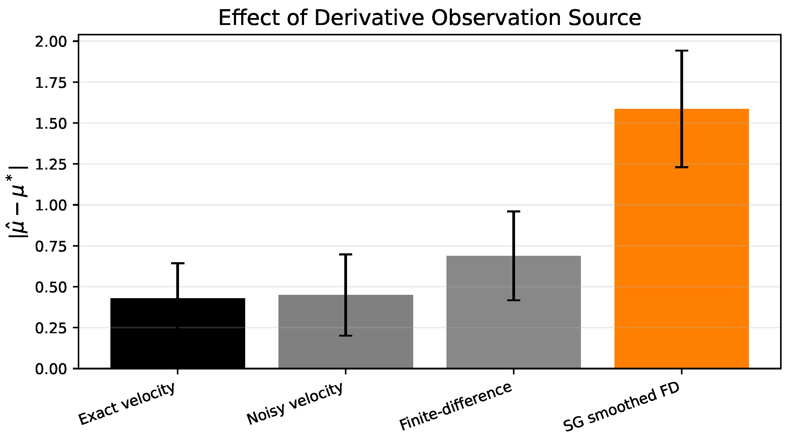
Exact and noisy velocity observations produce nearly identical results ( error vs. ), indicating that moderate Gaussian noise () in the velocity measurements does not significantly degrade D-PINN performance. Finite-difference derivatives computed from noisy displacement data increase error to (), and Savitzky–Golay smoothed finite differences further degrade performance to (). The SG filter, while reducing high-frequency noise in the displacement signal, appears to oversmooth the derivative estimate, removing genuine velocity variation that carries information about . These results suggest that direct velocity measurements (via laser Doppler vibrometry or accelerometer integration) are preferable when available, but finite-difference derivatives remain a viable alternative when only displacement sensors are available.
6.6. Discussion of Incomplete or Failed Experiments
The Wavelet PINN baseline from the original conference manuscript was excluded from this study because preliminary experiments showed inconsistent convergence behavior across seeds. The wavelet activation introduces additional trainable parameters (scale and shift) that interact unpredictably with the derivative observation loss, making fair comparison difficult. This baseline is superseded by the more principled gPINN and Sobolev-PINN baselines.
Bayesian uncertainty quantification (e.g., via Hamiltonian Monte Carlo or B-PINN [4]) is not implemented in the current study. While uncertainty estimates for would strengthen the identifiability analysis, they require substantially more computation and are left for future work.
7. Discussion
7.1. When Derivative Observations Help
The experimental results support a nuanced picture of when derivative observations improve parameter estimation:
- 1.
- Linear homogeneous systems with sparse displacement data. Derivative observations provide the largest benefit, reducing error by a factor of 3.4 without any prior. This is the regime where the parameter degeneracy identified in Section 3.3 is most severe.
- 2.
- Forced/nonlinear systems. Derivative observations provide important stabilization by preventing the catastrophic divergence observed with the standard PINN in the forced-vibration case. However, the absolute parameter errors remain larger than those in the homogeneous case.
- 3.
- Combined with a weak prior. The combination of derivative observations and a coarse prior (, deviation) achieves the best results across all three systems, reducing relative error to (linear), improving forced vibration stability, and achieving on the Duffing oscillator.
7.2. When Derivative Observations Do Not Help
- 1.
- Displacement fitting. Standard PINN already achieves displacement MSE of on the linear oscillator; D-PINN improves this only marginally in some cases. D-PINN should not be presented as a general-purpose accuracy improvement—its benefit is specifically in parameter estimation.
- 2.
- With poor-quality derivative estimates. When derivatives are obtained through Savitzky–Golay smoothing of noisy displacement data, D-PINN performance degrades below the no-derivative baseline.
- 3.
- Without Fourier features. D-PINN without Fourier features ( error ) performs nearly identically to standard PINN ( error ), indicating that the network must be capable of representing the oscillatory velocity signal for derivative supervision to be effective.
7.3. Limitations
- 1.
- Single-degree-of-freedom systems. The current study is limited to scalar second-order ODEs. Extension to multi-degree-of-freedom systems and partial differential equations requires further investigation.
- 2.
- Synthetic data. All experiments use synthetic data generated from known ODE solutions. Real experimental data would introduce model-form uncertainty (the governing equation may not be exact) and sensor-specific noise characteristics.
- 3.
- Hyperparameter sensitivity. The loss weights were tuned on the linear oscillator and applied unchanged to forced and Duffing systems. Adaptive loss balancing methods [12] may improve robustness across systems.
- 4.
- Computational cost. NLS achieves near-perfect results on these synthetic benchmarks with orders of magnitude less computation than D-PINN. The value proposition of D-PINN lies in scenarios where the forward model is uncertain, differentiability with respect to parameters is difficult to obtain, or the system is not expressible in closed form—scenarios not captured by the current synthetic benchmarks.
8. Conclusions
This paper proposed D-PINN, a derivative-observation-augmented physics-informed neural network for parameter identification in second-order dynamical systems, and provided a theoretical analysis of why derivative observations improve parameter identifiability. Three theoretical results, comprising a Sobolev-type error bound, a Fisher information decomposition, and a residual-based stability estimate, show that derivative supervision controls displacement error, contributes nonnegative information, and yields a tighter bound on the parameter estimation error.
Numerical experiments with 10 random seeds and 20,000 training epochs on three dynamical systems support the following conclusions:
- 1.
- D-PINN without any parameter prior reduces the damping coefficient relative error from (standard PINN) to , a 3.4-fold improvement attributable solely to derivative observations.
- 2.
- With a weak, non-oracle prior ( vs. true ), D-PINN achieves relative error, a 19-fold improvement over standard PINN, while maintaining a prior away from the true value.
- 3.
- The quality of derivative observations matters: finite-difference derivatives degrade performance by , and Savitzky–Golay smoothed derivatives degrade by relative to exact velocity measurements.
- 4.
- D-PINN provides critical stabilization for forced vibration near resonance, where standard PINN exhibits catastrophic divergence (some seeds exceeding relative error).
- 5.
- D-PINN does not improve displacement fitting accuracy in settings where standard PINN already achieves low MSE; its benefit is specifically in parameter estimation.
Future work includes extending the derivative observation framework to multi-degree-of-freedom systems, incorporating adaptive loss balancing for cross-system robustness, and validating D-PINN on experimental vibration data with real sensor noise and model-form uncertainty.
Author Contributions
Conceptualization, L.X.; methodology, L.X.; software, Y.L. and L.X.; validation, Y.L. and L.X.; formal analysis, L.X.; investigation, L.X. and Y.L.; resources, L.X.; data curation, Y.L.; writing—original draft preparation, L.X. and Y.L.; writing—review and editing, L.X.; visualization, Y.L.; supervision, L.X. All authors have read and agreed to the published version of the manuscript.
Funding
This research was supported in part by the Yuxiu Innovation Project of NCUT (Project No. 2024NCUTYXCX104.
Institutional Review Board Statement
Not applicable.
Informed Consent Statement
Not applicable.
Data Availability Statement
The code and experimental data supporting the reported results are available from the Liwen Xu’s Github repository: https://github.com/xulw2021-rgb/D-PINN.
Conflicts of Interest
The authors declare no conflicts of interest.
Abbreviations
The following abbreviations are used in this manuscript:
| PINN | Physics-Informed Neural Network |
| D-PINN | Derivative-Observation-Augmented PINN |
| gPINN | Gradient-Enhanced PINN |
| NLS | Nonlinear Least Squares |
| MSE | Mean Squared Error |
| MAE | Mean Absolute Error |
| FD | Finite Difference |
| SG | Savitzky–Golay |
| ODE | Ordinary Differential Equation |
Appendix A Oracle Prior Results (Diagnostic Only)
The following results use the oracle prior , which equals the true parameter value. These are presented solely as diagnostic references to characterize the method’s behavior when the exact parameter value is known, and must not be interpreted as practically achievable results. In any real application, the true parameter value is unknown by definition.
On the linear homogeneous oscillator, D-PINN with oracle prior () achieves error ( relative error). This result is worse than D-PINN with the weak prior ( error ), confirming that exact knowledge of the parameter value does not guarantee optimal performance in the composite PINN loss landscape. On the forced vibration system, the oracle prior achieves error ; on the Duffing oscillator, error .
These oracle results demonstrate that even with perfect prior knowledge, the PINN optimization does not trivially converge to the true parameter, underscoring the non-convex nature of the training objective and the importance of derivative observations in providing gradient signal toward .
References
- Raissi, M.; Perdikaris, P.; Karniadakis, G.E. Physics-informed neural networks: A deep learning framework for solving forward and inverse problems involving nonlinear partial differential equations. J. Comput. Phys. 2019, 378, 686–707. [Google Scholar] [CrossRef]
- Sun, L.; Gao, H.; Pan, S.; Wang, J.X. Surrogate modeling for fluid flows based on physics-constrained deep learning without simulation data. Comput. Methods Appl. Mech. Eng. 2020, 361, 112732. [Google Scholar] [CrossRef]
- Chen, Y.; Lu, L.; Karniadakis, G.E.; Dal Negro, L. Physics-informed neural networks for inverse problems in nano-optics and metamaterials. Opt. Express 2020, 28, 11618–11633. [Google Scholar] [PubMed]
- Yang, L.; Meng, X.; Karniadakis, G.E. B-PINNs: Bayesian physics-informed neural networks for forward and inverse PDE problems with noisy data. J. Comput. Phys. 2021, 425, 109913. [Google Scholar] [CrossRef]
- Wang, S.; Teng, Y.; Perdikaris, P. Understanding and mitigating gradient pathologies in physics-informed neural networks. SIAM J. Sci. Comput. 2021, 43, A3055–A3081. [Google Scholar] [CrossRef]
- Yu, J.; Lu, L.; Meng, X.; Karniadakis, G.E. Gradient-enhanced physics-informed neural networks for forward and inverse PDE problems. Comput. Methods Appl. Mech. Eng. 2022, 393, 114764. [Google Scholar] [CrossRef]
- Cui, X.; Xu, L.; Zhang, J. Review of research progress and applications of Physics-Informed Neural Networks (PINN). Adv. Mech. 2022, 52, 679–738. [Google Scholar]
- Wang, C.; Zhang, H.; Chen, L. Parameter identification of vibration systems using physics-informed neural networks under sparse data. Chin. J. Theor. Appl. Mech. 2024, 56, 456–468. [Google Scholar]
- Jagtap, A.D.; Kawaguchi, K.; Karniadakis, G.E. Adaptive activation functions accelerate convergence in deep and physics-informed neural networks. J. Comput. Phys. 2020, 404, 109136. [Google Scholar] [CrossRef]
- Wu, C.; Zhu, M.; Tan, Q.; Kartha, Y.; Lu, L. A comprehensive study of non-adaptive and residual-based adaptive sampling for physics-informed neural networks. Comput. Methods Appl. Mech. Eng. 2023, 403, 115671. [Google Scholar] [CrossRef]
- Gao, H.; Wang, J.X.; Zahr, M.J. Adaptive sampling for physics-informed neural networks via optimal transport. J. Comput. Phys. 2023, 485, 112080. [Google Scholar]
- Müller, J.; Zeinhofer, M. ReLoBRaLo: A robust local balancing method for multitask optimization in PINNs. J. Comput. Phys. 2024, 502, 112808. [Google Scholar]
- Xiang, Z.; Peng, W. Self-adaptive loss balanced physics-informed neural networks for solving PDEs. Neurocomputing 2022, 508, 1–14. [Google Scholar]
- Tancik, M.; Srinivasan, P.; Mildenhall, B.; Fridovich-Keil, S.; Raghavan, N.; Singhal, U.; Ramamoorthi, R.; Barron, J.; Ng, R. Fourier features let networks learn high frequency functions in low dimensional domains. Adv. Neural Inf. Process. Syst. 2020, 33, 7537–7547. [Google Scholar]
- Czarnecki, W.M.; Osindero, S.; Jaderberg, M.; Swirszcz, G.; Pascanu, R. Sobolev training for neural networks. Adv. Neural Inf. Process. Syst. 2017, 30, 4281–4290. [Google Scholar]
- Lai, Z.; Chen, Y.; Li, L.; Chatzi, E. A physics-informed deep neural network based beam vibration framework for simulation and parameter identification. Eng. Appl. Artif. Intell. 2025, 139, 109804. [Google Scholar]
- Zhang, Y.; Wang, J.; Liu, X. Bridge damping ratio identification based on function approximation-guided physics-informed neural networks. Structures 2025, 74, 108540. [Google Scholar]
- Gong, X.; Zhao, Y.; Li, H.; et al. Dynamic analysis of coal stick-slip impact based on physics-informed neural networks. Saf. Coal Mines 2023, 54, 112–118. [Google Scholar]
- Chen, X.; Yang, Y. FD-PINN: Frequency-domain physics-informed neural networks. Chin. J. Theor. Appl. Mech. 2023, 55, 1120–1132. [Google Scholar]
- Li, M.; Zhang, W.; Wang, L. Forward and inverse problems of nonlinear transient heat conduction based on physics-informed neural networks. J. Chongqing Univ. 2024, 47, 95–104. [Google Scholar]
- Liu, Y.; Chen, L. Vibration Mechanics, 3rd ed.; Higher Education Press: Beijing, China, 2018. [Google Scholar]
- Bao, W.; Bai, Q.; Lu, H. Fundamentals of Vibration Mechanics and MATLAB Applications; Tsinghua University Press: Beijing, China, 2015. [Google Scholar]
- Xu, Y. Mechanical System Dynamics; China Machine Press: Beijing, China, 1996. [Google Scholar]
- Zhang, X.; Xu, B.; He, J. Parameter identification method based on Kalman filtering and recursive least squares. Earthq. Eng. Eng. Vib. 2019, 39, 134–140. [Google Scholar]
- Hong, M. Research progress on optimal placement of piezoelectric elements in vibration control. Piezoelectr. Acoustoopt. 2015. [Google Scholar] [CrossRef]
- Zhao, H.; et al. Performance analysis of energy dissipation caused by vibration wave separation. J. Vib. Eng. 2023, 36, 1–10. [Google Scholar]
- Chen, W.; Wang, Q.; Hesthaven, J.S.; Zhang, C. Physics-informed machine learning for reduced-order modeling of nonlinear problems. J. Comput. Phys. 2021, 446, 110666. [Google Scholar] [CrossRef]
- Niaki, S.A.; Haghighat, E.; Campbell, T.; Poursartip, A.; Vaziri, R. Physics-informed neural network for modelling the thermochemical curing process of composite-tool systems during manufacture. Comput. Methods Appl. Mech. Eng. 2021, 384, 113959. [Google Scholar] [CrossRef]
- Huang, Y.; Tang, J.; Jiang, J.; et al. Identification and reinforcement learning control of nonlinear vibration systems using physics-informed neural networks. J. Vib. Eng. 2025, 38, 312–322. [Google Scholar]
- Liu, Y.; Sun, J.; Zhou, T. Adaptive sampling method for physics-informed neural networks guided by uncertainty quantification. Chin. J. Comput. Mech. 2025, 42, 45–53. [Google Scholar] [CrossRef]
Figure 1.
Displacement fitting and pointwise absolute error for forced vibration near resonance (, ). Standard PINN diverges catastrophically in some seeds ( error up to 85), while D-PINN maintains stable estimates. Results are from a representative seed.
Figure 1.
Displacement fitting and pointwise absolute error for forced vibration near resonance (, ). Standard PINN diverges catastrophically in some seeds ( error up to 85), while D-PINN maintains stable estimates. Results are from a representative seed.
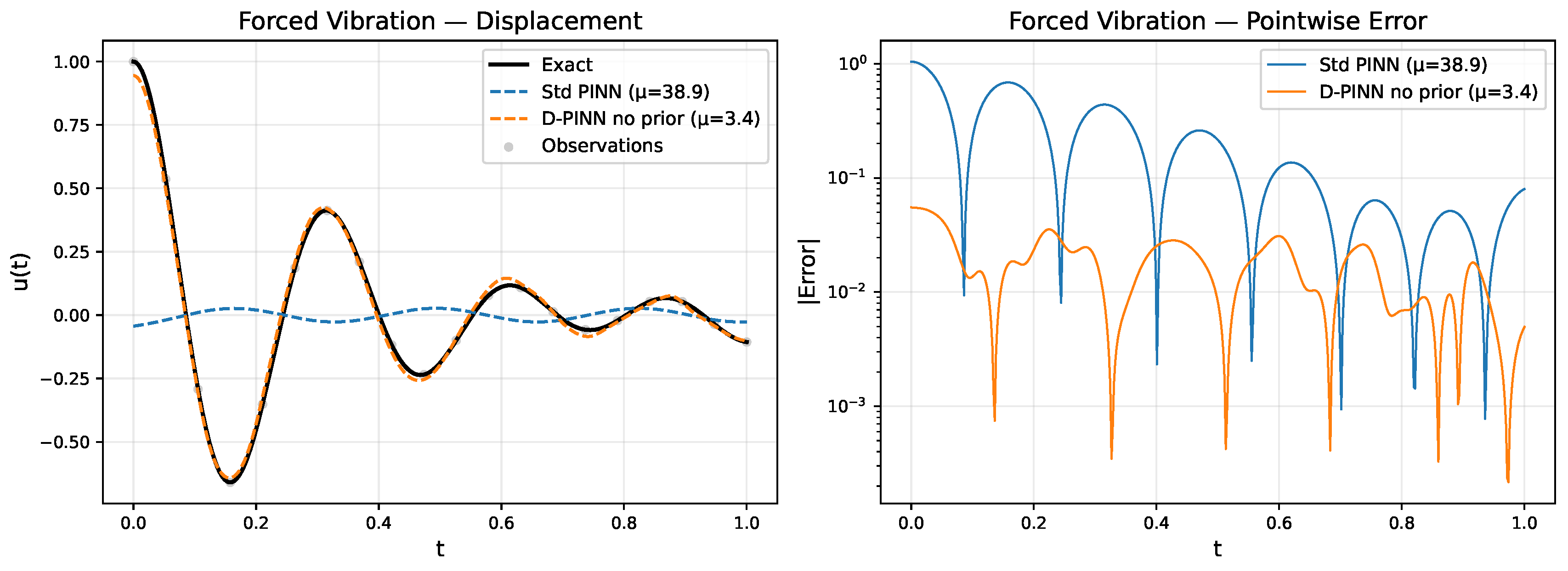
Figure 2.
Displacement fitting and pointwise absolute error for the Duffing oscillator (). The cubic nonlinearity introduces amplitude-dependent frequency shifts that weaken parameter identifiability, but D-PINN achieves lower error than standard PINN.
Figure 2.
Displacement fitting and pointwise absolute error for the Duffing oscillator (). The cubic nonlinearity introduces amplitude-dependent frequency shifts that weaken parameter identifiability, but D-PINN achieves lower error than standard PINN.
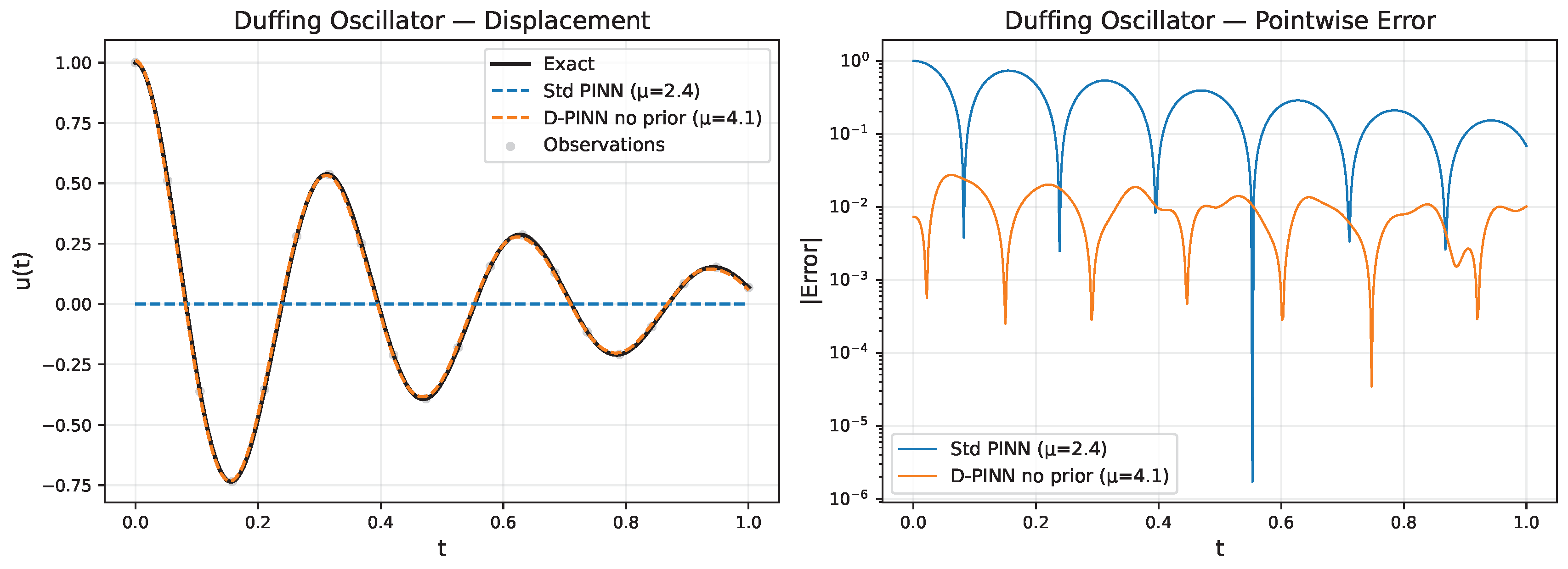
Figure 3.
Parameter estimation error as a function of the prior value (true ). Error bars show standard deviation over 10 seeds. Priors below the true value reduce error more effectively than priors above it, suggesting an asymmetric sensitivity landscape.
Figure 3.
Parameter estimation error as a function of the prior value (true ). Error bars show standard deviation over 10 seeds. Priors below the true value reduce error more effectively than priors above it, suggesting an asymmetric sensitivity landscape.
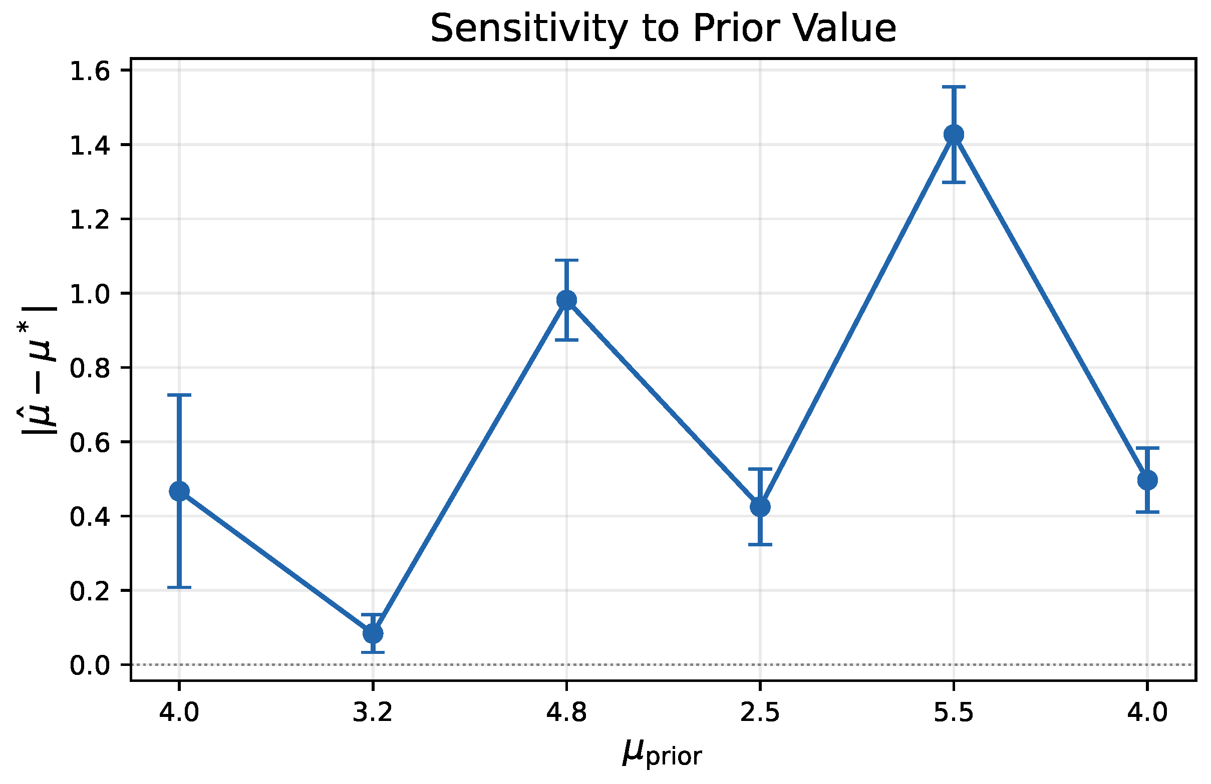

Table 1.
Method comparison on the linear underdamped oscillator. Mean ± standard deviation over 10 runs. No oracle prior is used in the main practical results.
Table 1.
Method comparison on the linear underdamped oscillator. Mean ± standard deviation over 10 runs. No oracle prior is used in the main practical results.
| Method | Disp. MSE | Disp. MAE | Error | Rel. Error (%) |
|---|---|---|---|---|
| NLS (classical) | ||||
| Standard PINN | ||||
| Fourier-PINN | ||||
| gPINN | ||||
| Sobolev-PINN | ||||
| D-PINN (no prior) | ||||
| D-PINN (no Fourier) | ||||
| D-PINN () | ||||
| D-PINN () | ||||
| D-PINN () | ||||
| D-PINN () | ||||
| D-PINN (oracle ) |
Table 2.
Ablation study: sensitivity of estimation to the parameter prior. Mean ± std over 10 runs. The oracle prior () is shown for reference; it must NOT be used in the main results.
Table 2.
Ablation study: sensitivity of estimation to the parameter prior. Mean ± std over 10 runs. The oracle prior () is shown for reference; it must NOT be used in the main results.
| Prior Setting | Error | ||
|---|---|---|---|
| No prior | |||
| Weak prior | |||
| Weak prior | |||
| Wrong prior | |||
| Wrong prior | |||
| Oracle prior | |||
| † Oracle prior (appendix only). | |||
Table 3.
Effect of derivative observation source on estimation accuracy. Displacement noise . Mean ± std over 10 runs.
Table 3.
Effect of derivative observation source on estimation accuracy. Displacement noise . Mean ± std over 10 runs.
| Derivative Source | Disp. MSE | Error | Rel. Error (%) |
|---|---|---|---|
| Exact velocity | |||
| Noisy velocity | |||
| Finite-difference | |||
| SG smoothed FD |
Disclaimer/Publisher’s Note: The statements, opinions and data contained in all publications are solely those of the individual author(s) and contributor(s) and not of MDPI and/or the editor(s). MDPI and/or the editor(s) disclaim responsibility for any injury to people or property resulting from any ideas, methods, instructions or products referred to in the content. |
© 2026 by the authors. Licensee MDPI, Basel, Switzerland. This article is an open access article distributed under the terms and conditions of the Creative Commons Attribution (CC BY) license (http://creativecommons.org/licenses/by/4.0/).
Copyright: This open access article is published under a Creative Commons CC BY 4.0 license, which permit the free download, distribution, and reuse, provided that the author and preprint are cited in any reuse.


