

Submitted:
23 July 2026
Posted:
23 July 2026
You are already at the latest version
Abstract
Simulation of the surface energy balance (SEB) is essential for land–atmosphere coupling and weather–climate prediction, yet land surface models remain uncertain in turbulent and ground heat fluxes. We evaluated CoLM2024 with Land Cover Type (LCT) and Plant Community (PC) schemes and ECLand v1.0 against energy-balance-corrected observations from 80 PLUMBER2 towers spanning 11 land cover types. Observations and simulations were decomposed at 30-min, daily, and monthly scales. All experiments reproduced net radiation well, whereas ground heat flux was poorly simulated over forests and wetlands because of excessive daytime amplitude, indicating limitations in canopy–soil heat partitioning and soil heat storage. ECLand achieved the best latent heat flux performance through smaller systematic errors. PC reduced unsystematic errors, but this benefit was offset by a large negative growing-season bias. Sensible heat flux performance depended on vegetation: PC performed best over evergreen needleleaf and mixed forests, while ECLand was superior over broadleaf forests and had the lowest unsystematic errors, although its implicit coupling damped variability. Performance was scale dependent: ECLand was favored at 30 min, PC was competitive for daily forest sensible heat correlations, and no consistent ranking emerged monthly. Complex canopy schemes therefore require robust formulations, improved heat-storage processes, and better parameter calibration.
Keywords:
land surface model
; surface energy balance
; land–atmosphere coupling
; PLUMBER2
; timescale decomposition
; vegetation-dependent bias
1. Introduction
Land surface models (LSMs) represent the exchanges of energy, water, and momentum between soil, vegetation, and the atmosphere. These exchanges govern near-surface thermodynamic states and boundary layer dynamics, providing indispensable lower-boundary forcing for atmospheric simulations that subsequently regulate cloud microphysics and precipitation regimes [1,2,3,4]. Beyond their foundational role in numerical weather prediction (NWP) and Earth system modeling (ESM), LSMs drive operational applications in water resource management, agricultural drought tracking, and ecosystem monitoring [5,6]. Consequently, the accurate simulation of the surface energy balance (SEB), which comprises net radiation, sensible and latent heat fluxes, and ground heat flux, is fundamental to LSM evaluation and critical for reducing uncertainty in coupled model predictions [7,8].
Discrepancies in SEB simulations typically originate from two interlinked sources: first, the representation of governing physical processes, such as canopy radiative transfer, canopy–atmosphere turbulent exchange, and soil heat and moisture transfer [9,10]; and second, the numerical algorithms governing equation discretization, temporal integration, and iterative closure [11,12]. Vegetation canopies, particularly forests, exacerbate these challenges due to their high aerodynamic roughness, low albedo, and intense transpiration. By regulating sensible and latent heat partitioning, forest canopies profoundly influence boundary layer thermodynamics, cloud-base height, and convective initiation [13,14]. Such intricate biophysical interactions routinely reveal structural deficiencies in LSM canopy schemes. For instance, Green et al. [15] quantified how vegetation-driven turbulent exchanges can elevate boundary layer depth and initiate convective systems, accounting for nearly a third of regional variability in precipitation and radiative budgets. Nevertheless, current LSMs and ESMs still struggle to capture the precise sensitivity of evapotranspiration to vegetation dynamics. A systematic evaluation of SEB simulations across diverse land covers (e.g., forested surfaces) is therefore essential for diagnosing and refining these model uncertainties.
Since the 1980s, LSMs have evolved from simple “bucket” schemes into complex systems that incorporate detailed canopy radiative transfer, turbulent exchange, soil water and heat transfer, and carbon cycle processes. Among existing LSMs, the Common Land Model (CoLM) and the ECMWF Land Surface Modelling System (ECLand) represent two distinct design philosophies. The prototype CoLM [1,16] integrated many leading LSM advances [17,18,19]. Subsequent iterations have steadily integrated higher-quality land surface datasets and more comprehensive process representations, enabling reliable numerical simulations across diverse spatial and temporal scales. As a result, CoLM has been widely adopted as a core component in operational weather forecasting, climate projection, and Earth system modeling frameworks [20,21,22,23,24,25]. Previous evaluations of CoLM have been largely site- or region-specific, primarily focusing on particular variables [26,27,28,29]. Zhang et al. [30] assessed surface energy fluxes across 20 FLUXNET sites at multiple timescales, finding the best performance over evergreen broadleaf forests and larger biases over croplands and wetlands. The latest CoLM2024 incorporates substantial refinements in surface flux simulations [31,32,33,34,35]—notably a three-dimensional canopy model and a plant hydraulic model—which together yield a more comprehensive representation of within-canopy energy and water exchange. These developments highlight the pressing need for a systematic, multi-site evaluation of CoLM2024 surface energy fluxes to fully assess its performance under diverse land covers.
ECLand [36], which forms part of the ECMWF Integrated Forecasting System, was developed by integrating hydrology, carbon cycle, and human activity modules into CHTESSEL (the Carbon-Hydrology Tiled Scheme for Surface Exchanges over Land) [37]. In contrast to CoLM’s detailed-physics pathway, the CHTESSEL family, which encompasses TESSEL [38], HTESSEL [39,40], and CHTESSEL, has been operational at ECMWF for more than 20 years, prioritizing numerical robustness and computational efficiency for operational applications. Key improvements in surface-flux-related processes include optimized soil hydrology [39,40], updated vegetation properties and leaf area index parameterizations [41,42], and single-layer and multi-layer snow schemes [43,44,45]. Evaluations of ECLand mostly concentrate on coupled land–atmosphere frameworks. Beljaars [46] diagnosed systematic errors in 2-m temperature and dewpoint during parameter optimization for the IFS, linking these model errors to snow cover, bare soil, and land–atmosphere coupling strength, while Martens et al. [47] assessed surface energy partitioning in ERA5 (whose land surface component is HTESSEL) and found a systematic overestimation of surface latent heat flux. However, offline evaluations of its surface energy fluxes and systematic comparisons with other LSMs across diverse land covers remain limited.
Beyond these diverging assessment histories, the two models also differ markedly in their physical structures and numerical formulations. Structurally, CoLM2024 resolves within-canopy energy exchange using one-dimensional and three-dimensional canopy models [31,33], whereas ECLand adopts a highly simplified canopy representation [36]. Numerically, CoLM2024 utilizes a Newton-Raphson iterative solver, while ECLand relies on a theoretically more stable implicit scheme [48]. These contrasts raise a key question: do detailed physical process representations versus simplified, numerically robust parameterizations produce systematically different SEB simulations, and are such differences driven by physics completeness or solver stability?
The PLUMBER2 dataset (Protocol for the Analysis of Land Surface Models Benchmarking Evaluation Project, phase 2), detailed by Abramowitz et al. [9], provides an ideal testbed for this comparison. Here, we benchmark CoLM2024 and ECLand v1.0 against flux observations from 80 PLUMBER2 sites spanning 11 land cover types and multiple global climate zones. Model performance is quantified using bias, linear correlation coefficient, root-mean-square error (decomposed into systematic and unsystematic components), and the index of agreement, examined at 30-min, daily, and monthly scales to resolve multi-scale error characteristics. Specifically, we ask whether the overall surface energy flux simulation is governed more by numerical robustness or by physical complexity, whether forest cover alters the performance ranking, and whether the relative error advantages of the two models are time-scale dependent. These findings provide quantitative evidence for optimizing canopy heat partitioning and numerical solvers, offering valuable guidance for model selection in predictions across spatiotemporal scales.
2. Materials and Methods
2.1. Model Descriptions
Land surface models commonly represent subgrid-scale heterogeneity in land cover by partitioning each model grid into multiple tiles or patches. CoLM2024 offers three alternative vegetation representations at the subgrid scale: Land Cover Type (LCT), Plant Functional Type (PFT), and Plant Community (PC). The LCT scheme, carried over from CoLM2014, allows individual patches to contain mixed vegetation types but applies uniform parameter values to all plant functional types within each patch [1,16,33]. Conversely, the PFT scheme aggregates vegetation of the same functional class across the grid cell into a single subgrid unit. Both the LCT and PFT configurations rely on a one-dimensional two-big-leaf framework to calculate surface radiation and turbulent fluxes.
The PC scheme extends the LCT framework by explicitly representing distinct PFTs within a vertically stratified canopy. Instead of aggregating vegetation into a single homogeneous layer, this configuration partitions the canopy into upper, middle, and lower strata, assigning an independent SEB equation to each level. These layer-specific equations are solved simultaneously to resolve vertical energy partitioning. From a computational standpoint, all three CoLM2024 configurations utilize a Newton iterative scheme to solve the SEB system. Because the LCT and PFT approaches share nearly identical physical formulations and numerical algorithms, this study focused exclusively on evaluating the LCT and PC configurations.
ECLand also utilizes a tile-based framework to represent subgrid heterogeneity, with its land cover classification broadly analogous to the PFT scheme in CoLM2024. However, in ECLand, the vegetation canopy is represented as an infinitesimally thin layer with negligible thickness. The SEB equation is formulated at this canopy interface, where canopy temperature is the surface skin temperature (Ts) and is thermally coupled to the uppermost soil layer through conductive heat transfer. ECLand addresses this coupling through an implicit numerical scheme that solves the SEB equation simultaneously with the vertical diffusion equation governing atmospheric turbulence [36,37,48]. This tightly integrated approach preserves numerical stability and maintains computational efficiency, particularly when using short time steps.
2.2. Experimental Setup
Atmospheric forcing data for the offline simulations were drawn from a globally distributed network of 90 high-quality flux tower sites. These data were quality controlled by Shi et al. [49] based on PLUMBER2 [50]. Both CoLM2024 and ECLand were integrated using a 30-min time step and cycled for 5 to 25 spin-up cycles depending on the length of the time series for the observations, ensuring a spin-up period exceeding 50 years for every site, with the final cycle of output retained for analysis at the native 30-min resolution.
Regarding static input data, CoLM2024 relied on a dedicated static data package developed by Shi et al. [49], which provides soil properties and vegetation characteristics tailored to this model version. In parallel, key static fields for ECLand were reprocessed from the original Shi et al. [49] dataset to match ECLand’s input format requirements, including reference height of wind (zuv) and temperature (zphista), soil types (sotype), high and low vegetation types and fractions (tvh, tvl, cvh, cvl), monthly leaf area index (Mlaih/Mlail). Variables unavailable in Shi et al. [49], such as monthly surface albedo (Malb) and surface roughness lengths (z0m and lz0h), were supplemented from the ERA5 global reanalysis at 0.25° × 0.25° resolution. The basis for creating the main static fields in ECLand is listed in Supplementary Table S1.
For initial conditions, CoLM2024 used the default values within the model, and ECLand was uniformly initialized across all sites using a standard test case distributed with the model. All remaining model configurations were kept at their default settings, and external modules representing river routing, human activities, and biogeochemical cycles were deactivated in both systems to isolate land-atmosphere exchange processes. Notably, the multi-layer snow scheme in ECLand remained in its default disabled state. Based on these configurations, three offline simulation experiments were conducted and are hereafter referred to as LCT, PC, and ECLand (Table 1).
The evaluation focused on four key components of the SEB: net radiation (Rnet), latent heat flux (HL), sensible heat flux (HS), and ground heat flux (HG). It is well established that the sum of sensible and latent heat fluxes measured by the eddy-covariance technique is systematically lower than the available energy (Rnet − HG), whereas land surface models are built upon energy conservation. The benchmark flux data were therefore derived from the energy-balance-corrected observations at 90 high-quality sites. To ensure robust statistical analysis, sites with extensive data gaps or anomalous values were further excluded. This screening yielded a final network of 80 sites with continuous, high-quality flux records spanning at least two years (Supplementary Table S3). Following the International Geosphere-Biosphere Programme (IGBP) land cover classification, these sites represent 11 typical surface types: cropland (CRO), deciduous broadleaf forest (DBF), evergreen broadleaf forest (EBF), evergreen needleleaf forest (ENF), wetlands (WET), woody savannas (WSA), grasslands (GRA), mixed forest (MF), open shrublands (OSH), closed shrublands (CSH), and savannas (SAV).
The geographic distribution of these sites and their associated climate zones is illustrated in Figure 1. Based on the Köppen-Geiger climate classification, the selected sites collectively span four major climate regions: tropical (A), arid (B), temperate (C), and cold (D). This broad climatic coverage, combined with the diversity of land cover types, provides a representative basis for evaluating model performance across heterogeneous terrestrial environments.
2.3. Evaluation Methods
To systematically diagnose model responses and error sources across temporal scales, we adopted the scale-decomposition approach proposed by Zhang et al. [30]. Original time series of observations and simulations (Xi) were decomposed into three components through temporal resampling: a monthly mean component (Xm), a daily anomaly component (Xd), and a residual component (Xs). Specifically, Xm represents monthly averages that capture seasonal variability. Xd is calculated as daily means after removing the monthly mean, reflecting day-to-day fluctuations such as those driven by synoptic-scale disturbances. Xs denotes the residual term after subtracting both Xm and Xd from Xi, representing rapid, local-scale processes. For the two sites US-Ne3 and US-MMS, where observed fluxes were recorded at hourly intervals, model outputs were similarly aggregated to hourly means to ensure consistency. These original and decomposed time series collectively form the basis for the comprehensive model evaluation presented in this study.
Model performance was assessed using a suite of statistical metrics, including normalized bias (Nbias), Pearson correlation coefficient (R), root-mean-square error (RMSE), and the index of agreement (IOA) proposed by Willmott [51]. RMSE was further decomposed into systematic (RMSEs) and unsystematic (RMSEu) components. The IOA provides an integrated measure of model-observation agreement and is generally more sensitive to overall model fidelity than the correlation coefficient alone. RMSEs reflects structural deficiencies in model physics that may be addressed through refined parameterizations or improved land surface datasets. In contrast, RMSEu represents random errors or noise associated with observational uncertainties, including errors in atmospheric forcing and eddy-covariance measurements, as well as numerical solver instability [51,52,53]. Definitions of all metrics are summarized in Table 2.
3. Results
3.1. Overall Performance and Error Decomposition of Simulated SEB
Figure 2 presents the evaluation results of the simulated SEB components against observational references across 11 land cover types. The performance metrics computed from the native 30-min resolution time series include the Index of Agreement (IOA) and Root Mean Square Error (RMSE), with systematic and unsystematic components denoted as RMSEs and RMSEu, respectively.
The index of agreement (IOA) for net radiation (Rnet) in all three experiments remains above 0.95 for all vegetation types, indicating excellent consistency between simulations and observations (Figure 2a). The RMSE generally ranges from approximately 20 to 40 W·m⁻², with RMSEu exceeding RMSEs for most land cover types and with comparable magnitudes among the three experiments (Figure 2b). These results suggest that all three schemes simulate radiative processes well over most vegetation types, with errors dominated by random perturbations such as uncertainties in atmospheric forcing data. The main exceptions occur for ECLand over evergreen needleleaf forest (ENF) and woody savannas (WSA), where total RMSE increases to approximately 50 and 45 W·m⁻², respectively. Over ENF, both systematic and unsystematic components contribute to the elevated error, whereas the WSA error is dominated by RMSEu.
Latent heat flux (HL) is generally well simulated, with the IOA mostly exceeding 0.75. Nevertheless, the IOA exhibits larger fluctuations across different vegetation types compared with Rnet (Figure 2c). Comprehensive evaluation based on IOA and RMSE shows that ECLand retains the best overall performance for HL across most land cover types. Its total error is generally dominated by RMSEu, whereas the PC scheme exhibits a larger RMSEs contribution over several vegetated surfaces, especially DBF. PC reduces RMSEu relative to LCT over all vegetation types, but this advantage is not uniform and is offset by large RMSEs. This suggests that parameter calibration remains the primary route for improving PC’s HL simulation.
The IOA results of sensible heat flux (HS) reveal that the performance of the three experiments is strongly dependent on land cover types (Figure 2e). Over wetlands (WET), all schemes reproduce HS less accurately than HL, with the IOA staying around 0.7 (Figure 2e), which is mainly caused by the generally high systematic error of HS over wetland surfaces (Figure 2f). Over areas with sparse vegetation, all three schemes yield satisfactory HS simulations, with the IOA ranging from 0.8 to 0.95, and their HS simulations outperforms those for HL. Across forested surfaces, however, no single experiment dominates. PC gives the highest IOA for ENF and MF, ECLand is comparable to PC over DBF and performs best over EBF, while LCT is generally less accurate. The corresponding RMSE ranking is similarly land-cover dependent: ECLand has the lowest or near-lowest RMSE over DBF and EBF, whereas PC retains an advantage over ENF and MF. Error decomposition further shows that the RMSEu of HS for the PC scheme is not generally lower than that of the LCT scheme, even over forested areas. This heterogeneous ranking indicates that canopy structural complexity alone does not determine HS performance.
Among all surface fluxes, ground heat flux (HG) is simulated worst by the three experiments, with considerable disparities across different land cover types (Figure 2g). Over forests and wetlands, HG simulation accuracy is extremely low, with the IOA generally below 0.5. In comparison, HG is better reproduced over sparsely vegetated areas, with the IOA between 0.7 and 0.9. The relatively small intermodel differences, compared with the sharp degradation from low vegetation to forests and wetlands, indicate a shared difficulty in representing canopy–soil heat partitioning and soil heat storage.
It is noteworthy that ECLand yields lower unsystematic error for HS than the two CoLM2024 schemes over most land cover types, including some forested areas. This may be attributed to its implicit algorithm to solve the SEB equation [48], which can suppress numerical oscillations that may arise in Newton iteration when atmospheric forcing changes rapidly under a large model time step [54]. However, this reduction in RMSEu is accompanied by an underestimation of HS variability (Figure 3i), indicating that numerical damping may suppress both spurious oscillations and part of the observed signal.
For HL, PC exhibits markedly lower RMSEu than LCT and, over some land covers, even lower than ECLand. This is physically consistent with the damping effect of the PC scheme’s multi-layer canopy structure, in which vertically stratified energy balance equations and inter-layer moisture redistribution introduce additional thermal and moisture inertia. This inertia buffers the canopy-atmosphere moisture exchange against rapidly varying atmospheric forcing, making the surface response more sluggish than in the single-layer LCT framework. Consequently, this multi-layer canopy structure also suppresses the model’s ability to capture rapidly varying signals, as evidenced by the systematically underestimated HL variability across all timescales (Figure 3e).
Comparison with a supplementary ECLand experiment driven by ERA5-derived land-surface attributes (Supplementary Figure S1) reveals that while harmonizing static inputs reduces both RMSEs and RMSEu, the most pronounced reductions occur in RMSEs—most notably for HS over CSH and forested surfaces. This indicates that mismatched soil and vegetation attributes are the dominant source of persistent systematic bias. In addition, the flux observations themselves are subject to considerable uncertainty, so the evaluation was repeated using the uncorrected HS and HL observations (Supplementary Figure S2). This test shows that observational uncertainty affects mainly the systematic errors of the models and has little influence on the unsystematic components. Taken together, these results indicate that the residual large RMSEu cannot be eliminated through parameter recalibration alone and should instead be attributed to atmospheric forcing uncertainty, physical process representation, and numerical solver behavior.
3.2. Multi-Timescale Performance and Scale-Dependent Errors
The models’ multi-timescale simulation capabilities and scale-dependent error characteristics at 30-min, daily, and monthly intervals are examined using Taylor diagrams, correlation coefficients, and RMSE. Rnet is simulated very well by all three experiments, with R values predominantly between 0.95 and 1.0. Compared with the evaluation of CoLM2014 by Zhang et al. [30], CoLM2024 shows substantially improved simulation of net radiation variability, as evidenced by SD values closer to the observed reference.
For HL, PC yields smaller variability than LCT (Figure 3d and Figure 3e), suggesting that the more complex canopy structure in PC suppresses the overly strong turbulent fluctuations present in the single-layer LCT framework. This statistical behavior is consistent with the physical interpretation in Section 3.1 that PC acts as a variability damper. Most notably, PC not only reduces the variability seen in LCT (daily SD occasionally exceeding 1.5), but also systematically underestimates HL variability across all timescales, with normalized SD values predominantly between 0.5 and 1.0 (Figure 3e). This suggests that the within-canopy moisture buffering is overly dissipative, causing the surface response to atmospheric forcing to be more sluggish than observed.
ECLand produces the smallest HS variability at all timescales (Figure 3i), with SD values mainly between 0.3 and 0.9, clearly lower than observations. This indicates that ECLand smooths sensible heat fluctuations excessively at all scales. In other words, the implicit coupling between the canopy interface and the atmospheric diffusion equation suppresses numerical noise while simultaneously smoothing out high-frequency real variance. Additionally, correlation performance at the 30-min scale surpasses that at the daily scale for all experiments, which may be explained by the temporal decomposition method, in which high-frequency residuals are isolated at the 30-min scale whereas systematic biases associated with synoptic variability are accentuated at the daily scale.
Figure 4 and Figure 5 respectively show the correlation coefficient (R) and RMSE of the simulated surface energy fluxes across the 11 land cover types at multiple timescales. In terms of correlation, the three experiments exhibit the smallest correlation coefficients at the daily scale; however, in terms of error magnitude, the RMSE for all fluxes at the 30-minute scale is higher than that at the daily and monthly scales. The two models differ in their simulation performance across timescales. At the 30-min scale, ECLand generally produces the highest correlations and lowest RMSE for HL and HS over most land cover types. This indicates that, although the implicit flux algorithm of ECLand suppresses part of the high-frequency signal and thereby underestimates HS variability (Figure 3i), it retains an advantage in simulating rapidly varying processes. The 30-min HL results of PC are noteworthy in this respect: over some forests (ENF and MF), PC yields a lower RMSE than ECLand but a lower correlation coefficient, and a similar contrast is found between PC and LCT. This again confirms that the multi-layer canopy of PC excessively dampens the high-frequency moisture exchange between the land surface and the atmosphere. At the daily scale, PC often gives higher HS correlations, particularly over DBF, ENF, and MF, whereas ECLand remains competitive in RMSE and retains a clear advantage for HL across many surfaces. At the monthly scale, the ranking becomes mixed: ECLand performs best across several forest and low-vegetation categories, whereas PC retains its advantages for ENF and MF but shows degraded performance for DBF. Rnet remains comparable among the experiments at all scales, except for larger ECLand RMSE over ENF and WSA, and no consistent model ranking is evident for HG. Therefore, relative performance depends jointly on flux component, land cover type, evaluation metric, and timescale.
3.3. Diurnal Contrast and Seasonal Variation
To further examine the distribution of simulation biases (including central tendency and variability) and their diurnal behavior, we computed the daytime and nighttime biases of each surface energy flux and visualized their full statistical distributions using boxplots (Figure 6). Furthermore, diurnal cycles of observed and simulated surface energy fluxes over four representative land cover types (DBF, ENF, GRA, SAV) are shown in Figure 7.
The daytime Rnet biases show that all three experiments underestimate net radiation over dense forest, including DBF, EBF, and ENF. The negative bias is largest in ECLand over ENF, where the median approaches −25 W·m−2 (Figure 6a) and the mean bias reaches approximately −80 W·m−2 at noon in summer (Figure 7b). Consistent with the elevated systematic error shown in Figure 2b, the systematic negative daytime bias of ECLand’s Rnet over ENF could be ameliorated by decreasing albedo or increasing canopy absorption of net short-wave radiation.
With regard to the partitioning of turbulent heat fluxes, LCT substantially overestimates daytime HL (Figure 6c) and underestimates daytime HS (Figure 6e) over forests (DBF, EBF, ENF, MF) and wetlands (WET), leading to a marked underestimation of the Bowen ratio (HS/HL). PC and ECLand reduce these opposing HL–HS biases over DBF and EBF, but PC substantially underestimates daytime HL over forests. The seasonal diurnal cycles confirm that the largest turbulent-flux discrepancies occur near midday in summer (Figure 7). It should be noted that the raw observed HS and HL are systematically lower than their energy-balance-corrected counterparts, particularly over forests, where the corrected summer maximum of HL is approximately 100 W·m⁻² larger than the uncorrected value (Supplementary Figure 7). Nevertheless, the daytime peak of the PC-simulated HL remains lower than both the raw and corrected observations, with a reduced diurnal amplitude. Its persistent negative HL bias is more consistent with excessive canopy resistance, insufficient effective evaporating area, or restrictive moisture availability, and these systematic controls should be calibrated before attributing the behavior to superior high-frequency filtering.
A consistent feature across all three experiments is the substantial overestimation of the HG amplitude (Figure 6g–h and 7m–o), which produces a systematic negative bias in daytime available surface energy (Rnet − HG), especially over some forest covers (Figure 6a,g). This indicates abnormal accumulation of heat within the soil profile by day and excessive release of stored heat overnight. Mechanistically, in both CoLM2024 and ECLand, HG is computed as the residual of the SEB equation (HG = Rnet − HL − HS); therefore, improving the simulations of HL and HS is essential for reducing the HG bias. Meanwhile, this bias is also likely attributable to oversimplified parameterizations of soil heat storage and conduction (i.e., soil heat capacity and thermal diffusivity), and it also reflects an overestimated coupling strength of energy exchange between the canopy and the underlying soil.
Annual cycles of surface fluxes are shown in Figure 8. ECLand retains a modest low bias in Rnet over ENF and some DBF and EBF groups, consistent with the daytime boxplot analysis, but the bias is not uniform across all forests. Over high-latitude mixed forest (MF:D), all three experiments overestimate warm-season Rnet, with the largest excess in PC, whereas the simulations over temperate mixed forest (MF:C) remain close to observations. This contrast suggests that errors in seasonal albedo and canopy development are climate-zone dependent rather than a single model-wide forest bias. It further indicates that the land cover classification scheme implemented in land surface models requires finer subdivision, particularly for complex landscapes with mixed vegetation types such as mixed forests (MF) and woody savannas (WSA).
The seasonal cycles of HL and HS reveal the largest errors over cold-climate forests across all experiments. In ENF:D and DBF:D, ECLand and LCT primarily underestimate the spring–summer HS amplitude, whereas PC may reproduce or overestimate HS during part of the growing season. Over MF:D, PC peaks later and higher than the observations, while ECLand follows the observed timing more closely but underestimates the amplitude. Concurrent HL biases also vary by scheme, with LCT generally high and PC often low over forests. These results indicate that the seasonal errors arise from coupled biases in phenology and LAI, stomatal and aerodynamic resistance, and soil-moisture limitation, rather than from phenological timing alone.
4. Discussion and Conclusions
This study evaluated the surface energy flux simulations of CoLM2024 and ECLand v1.0 against energy-balance-corrected observations from 80 PLUMBER2 flux-tower sites, with both observations and simulations decomposed at 30-min, daily, and monthly scales. The two models share several error characteristics. Net radiation is well reproduced over all 11 land cover types (IOA > 0.95), with errors dominated by unsystematic components associated with forcing uncertainty. Sensible and latent heat fluxes are generally well simulated (IOA mostly 0.7–0.9), although their accuracy depends strongly on land cover. Ground heat flux remains the most poorly simulated component over forests and wetlands (IOA < 0.5), despite reasonable performance over sparsely vegetated surfaces (IOA 0.7–0.9), and its dominant error—an excessive daytime amplitude in all experiments—points to persistent difficulties in representing canopy–soil heat partitioning and soil heat storage. All three experiments also share a common diurnal bias, with underestimated daytime sensible heat flux and overestimated daytime ground heat flux, indicating excessive daytime heat storage within the soil profile. The largest seasonal errors of turbulent fluxes occur over cold-climate forests, where they reflect coupled biases in vegetation phenology and LAI, canopy resistance, and soil-moisture limitation.
Beyond these shared features, the differences between the two models are informative. For latent heat flux, ECLand achieves the best overall performance, mainly because of its smaller systematic errors; the PC scheme reduces the unsystematic error relative to LCT and, over several forest types, even below that of ECLand, but this gain is offset by a large negative growing-season bias, leaving PC with the weakest overall HL performance. For sensible heat flux, no single experiment is superior across all forest types: PC performs best over ENF and MF, ECLand is comparable to PC over DBF and performs best over EBF, and LCT is generally the least accurate. ECLand yields the lowest unsystematic HS errors over most land cover types, which is consistent with the damping effect of its implicit coupling between the lowest model level variables and the corresponding surface fluxes; however, the same damping also suppresses part of the observed variability at all timescales (Figure 3i). A parallel effect occurs in PC, whose multi-layer canopy buffers canopy–atmosphere exchange and systematically underestimates HL variability (Figure 3e).
The relative performance of the two models further varies with timescale. At the 30-min scale, ECLand generally produces the highest correlations and the lowest RMSE for HL and HS, indicating that its implicit coupling remains effective for fast processes even though it smooths high-frequency variance. At the daily scale, PC gives higher HS correlations over several forest types, whereas ECLand remains competitive in RMSE and retains its advantage for HL. At the monthly scale, the ranking becomes mixed, with no experiment consistently superior. Consequently, a low RMSE does not by itself guarantee a realistic representation of variability, and conclusions drawn from a single metric or a single timescale can be misleading. The supplementary experiment driven by ERA5-derived land-surface attributes adds a further caution: harmonizing static inputs mainly reduces the systematic error components and can materially alter the apparent model ranking, consistent with Nogueira et al. [55], whereas the residual unsystematic errors are tied to forcing uncertainty, process representation, and solver behavior and cannot be removed through input harmonization alone.
These error patterns suggest several priorities for land surface model development. The persistent forest HG errors and the diurnal partitioning imbalance identify canopy–soil heat partitioning, including canopy and biomass heat storage and soil heat conduction as common targets; because HG is diagnosed as the residual of the surface energy balance, improving the HL and HS simulations is also a prerequisite for reducing HG biases. The systematic HL underestimation of PC indicates considerable room for parameter calibration, particularly of canopy resistance and moisture availability. The damped variability of ECLand suggests that numerical stability should not be pursued at the cost of excessive smoothing. The difficulty of big-leaf schemes in reproducing sensible and latent heat fluxes has been widely attributed to their simplified representation of vertical canopy structure—including radiation partitioning, within-canopy turbulent transport, canopy–atmosphere interactions, and understorey or mixed canopies—which has motivated the development of multi-layer canopy models [56]. The present comparison adds a numerical caveat to this physically motivated pathway: the additional canopy complexity of PC yields gains only for selected fluxes and forest types, whereas the implicit formulation of ECLand maintains robust performance across most conditions; therefore, complex canopy schemes should be developed in tandem with numerically robust solvers rather than through physical detail alone. An implicitly coupled multi-layer energy-balance scheme, as implemented in ORCHIDEE-CAN and ISBA-MEB [56,57,58], may combine the numerical robustness of ECLand with the physical detail of PC, and the present experiments provide a controlled benchmark for evaluating such a development.
Returning to the three questions posed in the Introduction, the following conclusions can be drawn. First, the overall simulation of surface energy fluxes is governed by neither numerical robustness nor physical complexity alone: once static inputs are harmonized, the physically simpler but numerically robust ECLand matches or outperforms the more detailed CoLM2024 configurations for most fluxes and metrics, and the additional canopy complexity of PC brings benefits only for selected fluxes and forest types, so that physical completeness does not translate directly into better flux simulations without adequate parameter calibration. Second, forest cover does alter the performance ranking: ECLand is generally preferable for HL and for HS over DBF and EBF, PC shows clear HS advantages over ENF and MF, and all schemes share large HG errors over forests and wetlands that are linked to canopy–soil heat partitioning and soil heat storage. Third, the relative error advantages of the two models are time-scale dependent, with ECLand favored at the 30-min scale, PC competitive in daily HS correlations over forests, and no consistent ranking at the monthly scale. These conclusions emphasize that benchmark evaluations should span multiple land cover types and timescales with harmonized inputs, and future work should examine how the identified surface flux biases propagate into boundary layer development, near-surface temperature variability, and weather–climate prediction in coupled modeling systems.
Supplementary Materials
The following supporting information can be downloaded at the website of this paper posted on Preprints.org, Tables S1 and S3 and Supplementary Figures S1, S2, and S7.
Author Contributions
Conceptualization, J.L., W.Z. and C.L.; methodology, J.L. and W.Z.; software, J.L.; formal analysis, J.L.; investigation, J.L.; data curation, J.L.; writing—original draft preparation, J.L.; writing—review and editing, W.Z., C.L. and B.W.; visualization, J.L.; supervision, W.Z. and C.L.; funding acquisition, W.Z. All authors have read and agreed to the published version of the manuscript.
Funding
This research was funded by the Natural Science Foundation of China, grant number 42405202.
Data Availability Statement
The input data and validation data for both CoLM2024 and ECLand were obtained directly or indirectly from Shi et al. (2025), which are publicly available at https://doi.org/10.5281/zenodo.12596218. Additional static fields for ECLand were supplemented from the ERA5 global reanalysis product, publicly available through the Copernicus Climate Change Service (C3S) Climate Data Store (https://cds.climate.copernicus.eu/). The ECLand static data files generated in this study are available from the corresponding author upon reasonable request.
Conflicts of Interest
The authors declare no conflicts of interest.
References
- Dai, Y.; Zeng, X.; Dickinson, R.E.; Baker, I.; Bonan, G.B.; Bosilovich, M.G.; et al. The Common Land Model. Bull. Am. Meteorol. Soc. 2003, 84, 1013–1024. [Google Scholar] [CrossRef]
- Niu, G.Y.; Yang, Z.L.; Mitchell, K.E.; et al. The community Noah land surface model with multiparameterization options (Noah-MP): 1. Model description and evaluation with local-scale measurements. J. Geophys. Res. 2011, 116, D12109. [Google Scholar] [CrossRef]
- Yang, Z.L.; Niu, G.Y.; Mitchell, K.E.; et al. The community Noah land surface model with multiparameterization options (Noah-MP): 2. Evaluation over global river basins. J. Geophys. Res. 2011, 116, D12110. [Google Scholar] [CrossRef]
- Best, M.J.; Pryor, M.; Clark, D.B.; Rooney, G.G.; Essery, R.L.H.; Menard, C.B.; et al. The Joint UK Land Environment Simulator (JULES), model description – Part 1: Energy and water fluxes. Geosci. Model Dev. 2011, 4, 677–699. [Google Scholar] [CrossRef]
- Pan, X.; Chen, D.; Pan, B.; Huang, X.; Yang, K.; Piao, S.; Zhou, T.; Dai, Y.; Chen, F.; Li, X. Evolution and prospects of Earth system models: challenges and opportunities. Earth-Sci. Rev. 2025, 260, 104986. [Google Scholar] [CrossRef]
- Blyth, E.M.; Arora, V.K.; Clark, D.B.; Dadson, S.J.; De Kauwe, M.G.; Lawrence, D.M.; Melton, J.R.; Pongratz, J.; Turton, R.H.; Yoshimura, K.; Yuan, H. Advances in land surface modelling. Curr. Clim. Chang. Rep. 2021, 7, 45–71. [Google Scholar] [CrossRef]
- Wei, Z.; Xu, Q.; Bai, F.; Xu, X.; Wei, Z.; Dong, W.; Liang, H.; Wei, N.; Lu, X.; Li, L.; Zhang, S.; Yuan, H.; Liu, L.; Dai, Y. OpenBench: a land model evaluation system. Geosci. Model Dev. 2025, 18, 6517–6540. [Google Scholar] [CrossRef]
- Zarakas, C.M.; Kennedy, D.; Dagon, K.; Lawrence, D.M.; Liu, A.; Bonan, G.; Koven, C.; Lombardozzi, D.; Swann, A.L.S. Land processes can substantially impact the mean climate state. Geophys. Res. Lett. 2024, 51, e2024GL108372. [Google Scholar] [CrossRef]
- Abramowitz, G.; Ukkola, A.; Hobeichi, S.; Cranko Page, J.; Lipson, M.; De Kauwe, M.G.; et al. On the predictability of turbulent fluxes from land: PLUMBER2 MIP experimental description and preliminary results. Biogeosciences 2024, 21, 5517–5538. [Google Scholar] [CrossRef]
- Best, M.J.; Abramowitz, G.; Johnson, H.R.; Pitman, A.J.; Balsamo, G.; Boone, A.; et al. The Plumbing of Land Surface Models: benchmarking model performance. J. Hydrometeorol. 2015, 16, 1425–1442. [Google Scholar] [CrossRef]
- Clark, M.P.; Zolfaghari, R.; Green, K.R.; Trim, S.J.; Knoben, W.J.M.; Bennett, A.R.; Nijssen, B.; Ireson, A.M.; Spiteri, R.J. The numerical implementation of land models: problem formulation and laugh tests. J. Hydrometeorol. 2021, 22, 1627–1648. [Google Scholar] [CrossRef]
- Mauder, M.; Foken, T.; Cuxart, J. Surface-energy-balance closure over land: a review. Bound.-Layer. Meteorol. 2020, 177, 395–426. [Google Scholar] [CrossRef]
- Teuling, A.J.; Taylor, C.M.; Meirink, J.F.; et al. Observational evidence for cloud cover enhancement over western European forests. Nat. Commun. 2017, 8, 14065. [Google Scholar] [CrossRef] [PubMed]
- Duveiller, G.; Filipponi, F.; Ceglar, A.; Bojanowski, J.; Alkama, R.; Cescatti, A. Revealing the widespread potential of forests to increase low level cloud cover. Nat. Commun. 2021, 12, 4337. [Google Scholar] [CrossRef] [PubMed]
- Green, J.K.; Konings, A.G.; Alemohammad, S.H.; Berry, J.; Entekhabi, D.; Kolassa, J.; Lee, J.E.; Gentine, P. Regionally strong feedbacks between the atmosphere and terrestrial biosphere. Nat. Geosci. 2017, 10, 410–414. [Google Scholar] [CrossRef] [PubMed]
- Dai, Y.; Dickinson, R.E.; Wang, Y.P. A two-big-leaf model for canopy temperature, photosynthesis, and stomatal conductance. J. Clim. 2004, 17, 2281–2299. [Google Scholar] [CrossRef]
- Dickinson, R.E.; Henderson-Sellers, A.; Kennedy, P.J. Biosphere-Atmosphere Transfer Scheme (BATS) Version 1e as Coupled to the NCAR Community Climate Model. In NCAR Tech. Note; National Center for Atmospheric Research: Boulder, CO, 1993. [Google Scholar]
- Bonan, G.B. A Land Surface Model (LSM Version 1.0) for Ecological, Hydrological, and Atmospheric Studies: Technical Description and User’s Guide; NCAR Tech. Note, National Center for Atmospheric Research: Boulder, CO, 1996. [Google Scholar] [CrossRef]
- Dai, Y.; Zeng, Q. A land surface model (IAP94) for climate studies. Part I: Formulation and validation in off-line experiment. Adv. Atmos. Sci. 1997, 14, 433–460. [Google Scholar] [CrossRef]
- Yuan, X.; Liang, X.Z. Improving cold season precipitation prediction by the nested CWRF-CFS system. Geophys. Res. Lett. 2011, 38, L02706. [Google Scholar] [CrossRef]
- Liang, X.Z.; Xu, M.; Yuan, X.; Ling, T.; Choi, H.I.; Zhang, F.; Chen, L.; Liu, S.; Su, S.; Qiao, F.; et al. Regional Climate-Weather Research and Forecasting Model. Bull. Am. Meteorol. Soc. 2012, 93, 1363–1387. [Google Scholar] [CrossRef]
- Ji, D.; Wang, L.; Feng, J.; Wu, Q.; Cheng, H.; Zhang, Q.; et al. Description and basic evaluation of Beijing Normal University Earth System Model (BNU-ESM) version 1. Geosci. Model Dev. 2014, 7, 2039–2064. [Google Scholar] [CrossRef]
- Shen, X.; Su, Y.; Hu, J.; Wang, J.; Sun, J.; Xue, J.; Han, W.; Zhang, H.; Lu, H.; Zhang, H.; et al. Development and operation transformation of GRAPES global middle-range forecast system. J. Appl. Meteorol. Sci. 2017, 28, 1–10. [Google Scholar] [CrossRef]
- Yuan, Z.; Wei, N. Coupling a new version of the Common Land Model (CoLM) to the Global/Regional Assimilation and Prediction System (GRAPES): implementation, experiment, and preliminary evaluation. Land 2022, 11, 770. [Google Scholar] [CrossRef]
- Zhu, J.; Zeng, X.; Zhang, M.; Dai, Y.; Ji, D.; Li, F.; Zhang, Q.; Zhang, H.; Song, X. Evaluation of the new dynamic global vegetation model in CAS-ESM. Adv. Atmos. Sci. 2018, 35, 659–670. [Google Scholar] [CrossRef]
- Xu, T.R.; Liu, S.M.; Liang, S.L.; Qin, J. Improving predictions of water and heat fluxes by assimilating MODIS land surface temperature products into the Common Land Model. J. Hydrometeorol. 2011, 12, 227–244. [Google Scholar] [CrossRef]
- Whitfield, B.; Jacobs, J.M.; Judge, J. Intercomparison study of the Land Surface Process Model and the Common Land Model for a prairie wetland in Florida. J. Hydrometeorol. 2006, 7, 1247–1258. [Google Scholar] [CrossRef]
- Leng, P.; Song, X.N.; Li, Z.L.; Wang, Y.W. Evaluation of the effects of soil layer classification in the Common Land Model on modeled surface variables and the associated land surface soil moisture retrieval model. Remote Sens. 2013, 5, 5514–5529. [Google Scholar] [CrossRef]
- Zhang, G.; Zhang, Y.; Lu, Y.; Cao, X.; Cai, X.; Yang, K.; et al. Decomposition and attribution of land surface temperature bias over China in CoLMv2024 and Noah-MP land surface model. J. Geophys. Res. Atmos. 2025, 130, e2025JD044230. [Google Scholar] [CrossRef]
- Zhang, X.; Dai, Y.; Cui, H.; Dickinson, R.E.; Zhu, S.; Wei, N.; Yan, B.; Yuan, H.; Shangguan, W.; Wang, L.; Fu, W. Evaluating Common Land Model energy fluxes using FLUXNET data. Adv. Atmos. Sci. 2017, 34, 1035–1046. [Google Scholar] [CrossRef]
- Yuan, H.; Dickinson, R.E.; Dai, Y.; Shaikh, M.J.; Zhou, L.; Shangguan, W.; Ji, D. A 3D canopy radiative transfer model for global climate modeling: description, validation, and application. J. Clim. 2014, 27, 1168–1192. [Google Scholar] [CrossRef]
- Yuan, H.; Dai, Y.; Dickinson, R.E.; Pinty, B.; Shangguan, W.; Zhang, S.; Wang, L.; Zhu, S. Reexamination and further development of two-stream canopy radiative transfer models for global land modeling. J. Adv. Model. Earth Syst. 2017, 9, 113–129. [Google Scholar] [CrossRef]
- Dai, Y.; Yuan, H.; Xin, Q.; Wang, D.; Shangguan, W.; Zhang, S.; Liu, S.; Wei, N. Different representations of canopy structure – A large source of uncertainty in global land surface modeling. Agric. For. Meteorol. 2019, 269–270, 119–135. [Google Scholar] [CrossRef]
- Liu, S.; Zeng, X.; Dai, Y.; Shao, Y. Further improvement of surface flux estimation in the unstable surface layer based on large-eddy simulation data. J. Geophys. Res. Atmos. 2019, 124, 9839–9854. [Google Scholar] [CrossRef]
- Liu, S.; Zeng, X.; Dai, Y.; et al. A surface flux estimation scheme accounting for large-eddy effects for land surface modeling. Geophys. Res. Lett. 2022, 49, e2022GL101754. [Google Scholar] [CrossRef]
- Boussetta, S.; Balsamo, G.; Arduini, G.; Dutra, E.; McNorton, J.; Choulga, M.; et al. ECLand: the ECMWF Land Surface Modelling System. Atmosphere 2021, 12, 723. [Google Scholar] [CrossRef]
- Boussetta, S.; Balsamo, G.; Beljaars, A.; Agusti-Panareda, A.; Calvet, J.; Jacobs, C.; et al. Natural land carbon dioxide exchanges in the ECMWF Integrated Forecasting System: implementation and offline validation. J. Geophys. Res. Atmos. 2013, 118, 5923–5946. [Google Scholar] [CrossRef]
- van den Hurk, B.J.J.M.; Viterbo, P.; Beljaars, A.C.M.; Betts, A.K. Offline validation of the ERA40 surface scheme. ECMWF Tech. Memo. 2000, 295. [Google Scholar]
- Balsamo, G.; Beljaars, A.; Scipal, K.; Viterbo, P.; van den Hurk, B.; Hirschi, M.; Betts, A.K. A revised hydrology for the ECMWF model: verification from field site to terrestrial water storage and impact in the Integrated Forecast System. J. Hydrometeorol. 2009, 10, 623–643. [Google Scholar] [CrossRef]
- Balsamo, G.; Boussetta, S.; Dutra, E.; Beljaars, A.; Viterbo, P.; van den Hurk, B. Evolution of land-surface processes in the IFS. ECMWF Newsl. 2011, 127, 17–22. [Google Scholar]
- van Oorschot, F.; van der Ent, R.J.; Hrachowitz, M.; et al. Interannual land cover and vegetation variability based on remote sensing data in the HTESSEL land surface model: implementation and effects on simulated water dynamics. Earth Syst. Dyn. 2023, 14, 1239–1259. [Google Scholar] [CrossRef]
- Ruiz-Vásquez, M.; O, S.; Arduini, G.; Boussetta, S.; Brenning, A.; Bastos, A.; et al. Impact of updating vegetation information on land surface model performance. J. Geophys. Res. Atmos. 2023, 128, e2023JD039076. [Google Scholar] [CrossRef]
- Dutra, E.; Balsamo, G.; Viterbo, P.; Miranda, P.M.A.; Beljaars, A.; Schär, C.; Elder, K. New snow scheme in HTESSEL: description and offline validation. ECMWF Tech. Memo. 2009, 607. [Google Scholar]
- Dutra, E.; Balsamo, G.; Viterbo, P.; Miranda, P.M.A.; Beljaars, A.; Schär, C.; Elder, K. An improved snow scheme for the ECMWF land surface model: description and offline validation. J. Hydrometeorol. 2010, 11, 899–916. [Google Scholar] [CrossRef]
- Arduini, G.; Balsamo, G.; Dutra, E.; Day, J.J.; Sandu, I.; Boussetta, S.; Haiden, T. Impact of a multi-layer snow scheme on near-surface weather forecasts. J. Adv. Model. Earth Syst. 2019, 11, 4687–4710. [Google Scholar] [CrossRef]
- Beljaars, A. Towards optimal parameters for the prediction of near surface temperature and dewpoint. ECMWF Tech. Memo. 2020, 868. [Google Scholar]
- Martens, B.; Schumacher, D.L.; Wouters, H.; Muñoz-Sabater, J.; Verhoest, N.E.C.; Miralles, D.G. Evaluating the land-surface energy partitioning in ERA5. Geosci. Model Dev. 2020, 13, 4159–4181. [Google Scholar] [CrossRef]
- Best, M.J.; Beljaars, A.; Polcher, J.; Viterbo, P. A proposed structure for coupling tiled surfaces with the planetary boundary layer. J. Hydrometeorol. 2004, 5, 1271–1278. [Google Scholar] [CrossRef]
- Shi, J.; Yuan, H.; Lin, W.; Dong, W.; Liang, H.; Liu, Z.; Zeng, J.; Zhang, H.; Wei, N.; Wei, Z.; Zhang, S.; Liu, S.; Lu, X.; Dai, Y. A flux tower site attribute dataset intended for land surface modeling. Earth Syst. Sci. Data 2025, 17, 117–134. [Google Scholar] [CrossRef]
- Ukkola, A. M.; Abramowitz, G.; De Kauwe, M. G. A flux tower dataset tailored for land model evaluation. Earth Syst. Sci. Data 2022, 14, 449–461. [Google Scholar] [CrossRef]
- Willmott, C.J. Some comments on the evaluation of model performance. Bull. Am. Meteorol. Soc. 1982, 63, 1309–1313. [Google Scholar] [CrossRef]
- Mauder, M.; Foken, T. Impact of post-field data processing on eddy covariance flux estimates and energy balance closure. Meteorol. Z. 2006, 15, 597–609. [Google Scholar] [CrossRef] [PubMed]
- Durand, P. A possible reconciliation between eddy covariance fluxes and surface energy balance closure. Atmosphere 2022, 13. [Google Scholar] [CrossRef]
- Schulz, J.; Dümenil, L. J. Polcher, 2001: On the land surface–atmosphere coupling and its impact in a single–column atmospheric model. J. Appl. Meteorol. Climatol. 40, 642–663. [CrossRef]
- Nogueira, M.; Boussetta, S.; Balsamo, G.; Albergel, C.; Trigo, I.F.; Johannsen, F.; Miralles, D.G.; Dutra, E. Upgrading land-cover and vegetation seasonality in the ECMWF coupled system: verification with FLUXNET sites, METEOSAT satellite land surface temperatures, and ERA5 atmospheric reanalysis. J. Geophys. Res. Atmos. 2021, 126, e2020JD034163. [Google Scholar] [CrossRef] [PubMed]
- Ryder, J.; Polcher, J.; Peylin, P.; Ottlé, C.; Chen, Y.; van Gorsel, E.; et al. A multi-layer land surface energy budget model for implicit coupling with global atmospheric simulations. Geosci. Model Dev. 2016, 9, 223–245. [Google Scholar] [CrossRef]
- Chen, Y.; Ryder, J.; Bastrikov, V.; Polcher, J.; Peylin, P.; Ottlé, C.; et al. Evaluating the performance of land surface model ORCHIDEE-CAN v1.0 on water and energy flux estimation with a single- and multilayer energy budget scheme. Geosci. Model Dev. 2016, 9, 2951–2972. [Google Scholar] [CrossRef]
- Boone, A.; Samuelsson, P.; Gollvik, S.; Napoly, A.; Jarlan, L.; Brun, E.; et al. The interactions between soil–biosphere–atmosphere land surface model with a multi-energy balance (ISBA-MEB) option in SURFEXv8 – Part 1: Model description. Geosci. Model Dev. 2017, 10, 843–872. [Google Scholar] [CrossRef]
- Wösten, J. H. M.; Lilly, A.; Nemes, A.; et al. Development and use of a database of hydraulic properties of European soils. Geoderma 1999, 90(3−4), 169−185. [Google Scholar] [CrossRef]
Figure 1.
Spatial distribution of flux tower sites across Köppen-Geiger climate zones.
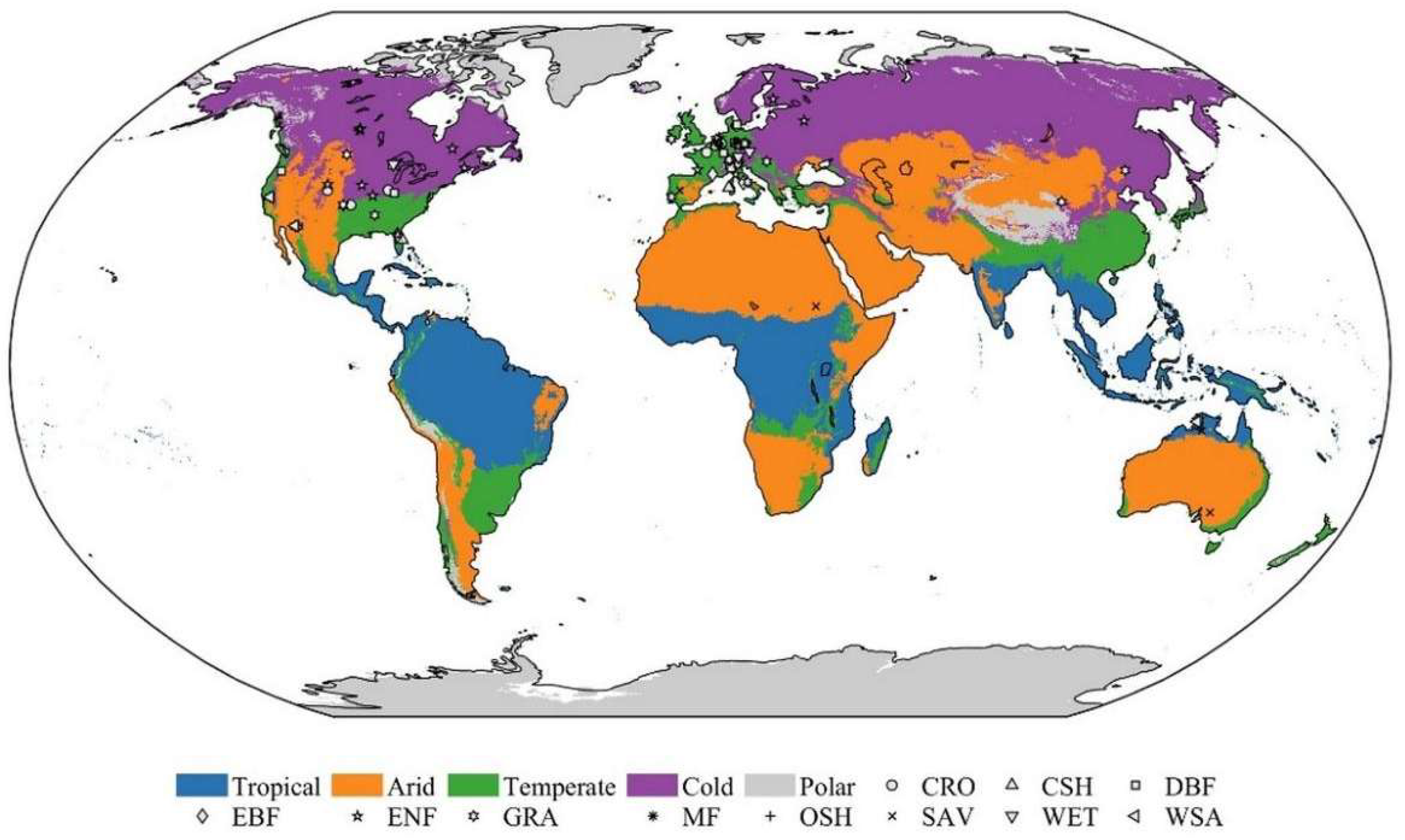
Figure 2.
Index of Agreement (IOA) and RMSE (including systematic RMSEs and unsystematic RMSEu) across 11 land cover types for the LCT, PC, and ECLand experiments.
Figure 2.
Index of Agreement (IOA) and RMSE (including systematic RMSEs and unsystematic RMSEu) across 11 land cover types for the LCT, PC, and ECLand experiments.
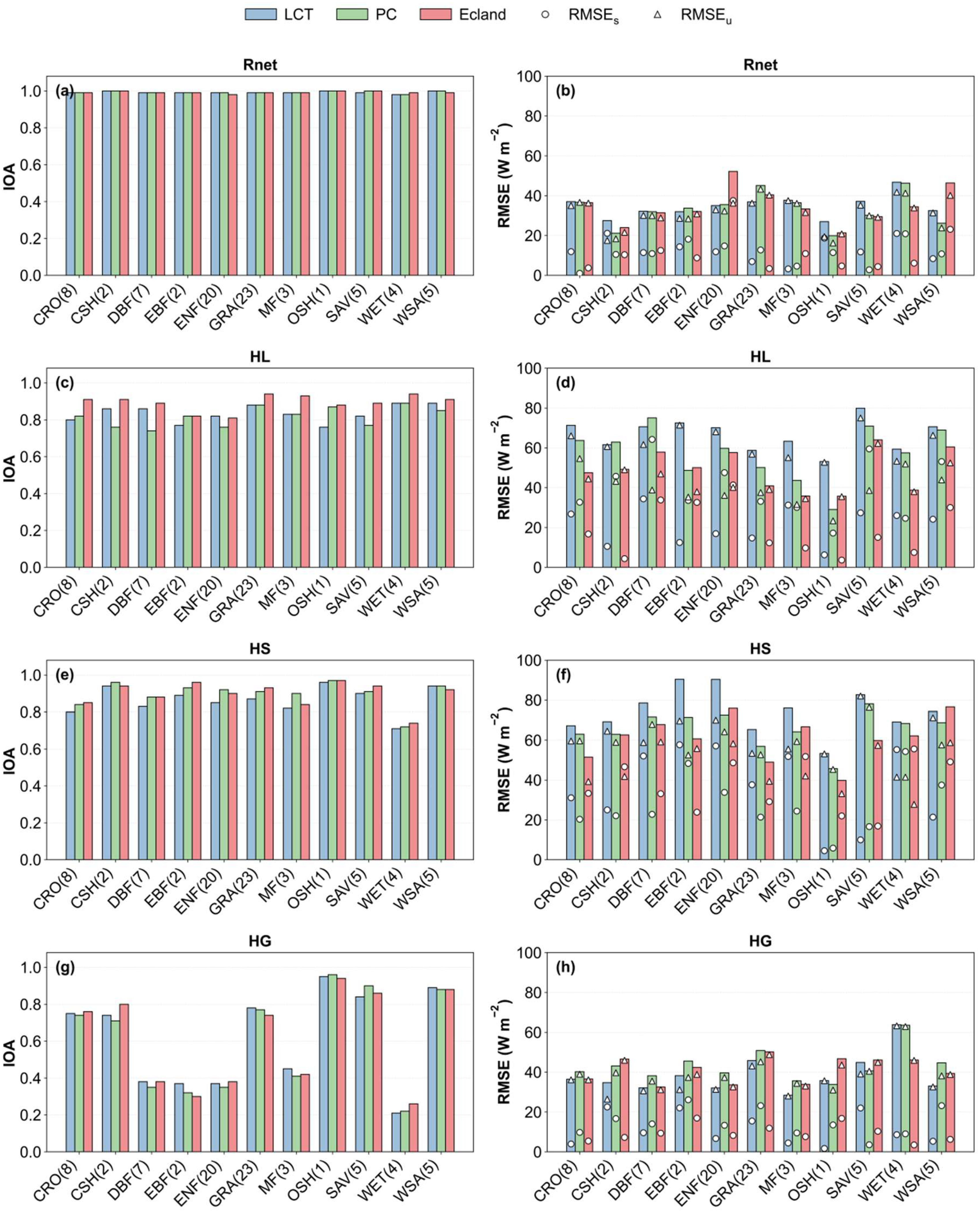
Figure 3.
Taylor diagrams of Rnet, HL, and HS simulated by the LCT, PC, and ECLand experiments at 30-minute, daily, and monthly timescales.
Figure 3.
Taylor diagrams of Rnet, HL, and HS simulated by the LCT, PC, and ECLand experiments at 30-minute, daily, and monthly timescales.
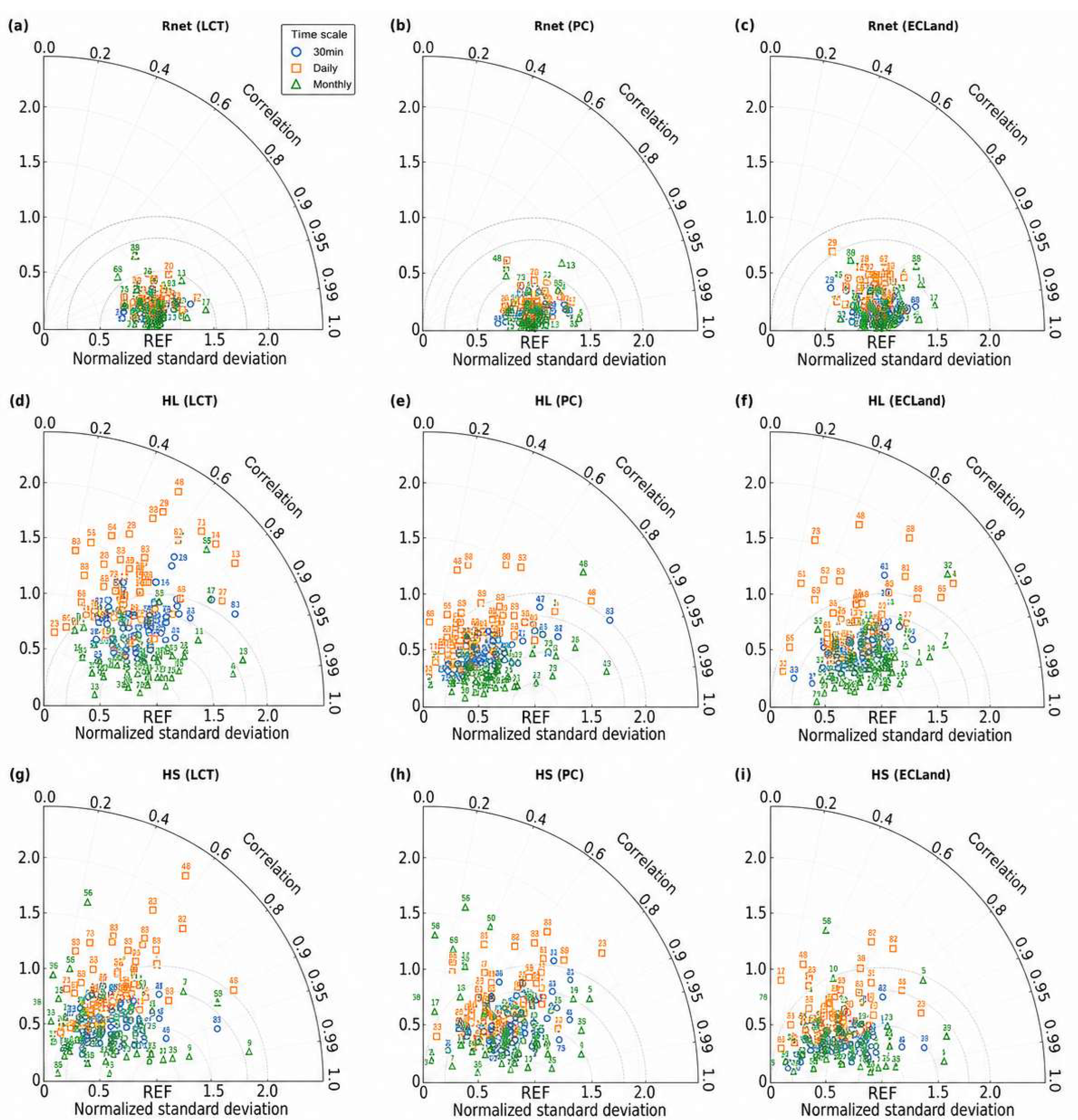
Figure 4.
Correlation coefficients (R) between simulated and observed surface energy fluxes for the LCT, PC, and ECLand experiments across 11 land cover types at 30-minute, daily, and monthly scales.
Figure 4.
Correlation coefficients (R) between simulated and observed surface energy fluxes for the LCT, PC, and ECLand experiments across 11 land cover types at 30-minute, daily, and monthly scales.
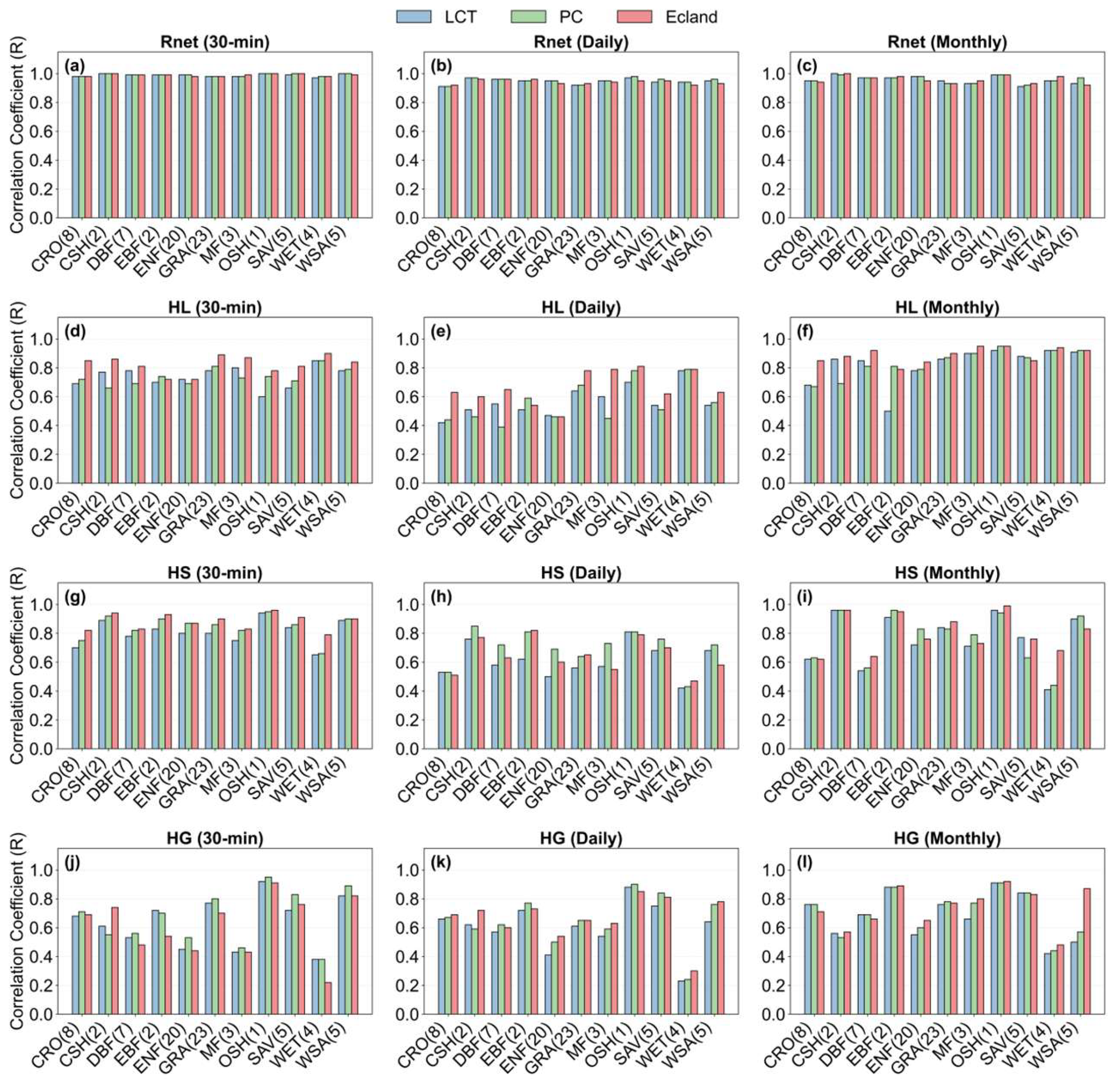
Figure 5.
RMSE of simulated SEB components (Rnet, HL, HS and HG) for the LCT, PC, and ECLand experiments across 11 land cover types at different timescales.
Figure 5.
RMSE of simulated SEB components (Rnet, HL, HS and HG) for the LCT, PC, and ECLand experiments across 11 land cover types at different timescales.
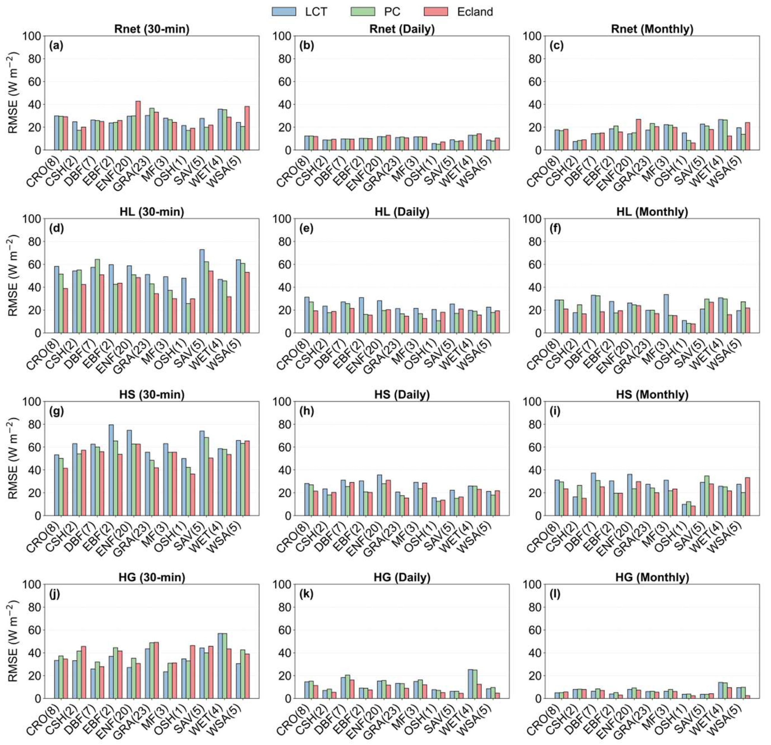
Figure 6.
Boxplots of biases in simulated surface energy fluxes (net radiation Rnet, sensible heat flux HS, latent heat flux HL, and ground heat flux HG) against site observations for three numerical experiments (LCT, PC, and ECLand) under different land cover types, shown separately for daytime and nighttime conditions.
Figure 6.
Boxplots of biases in simulated surface energy fluxes (net radiation Rnet, sensible heat flux HS, latent heat flux HL, and ground heat flux HG) against site observations for three numerical experiments (LCT, PC, and ECLand) under different land cover types, shown separately for daytime and nighttime conditions.
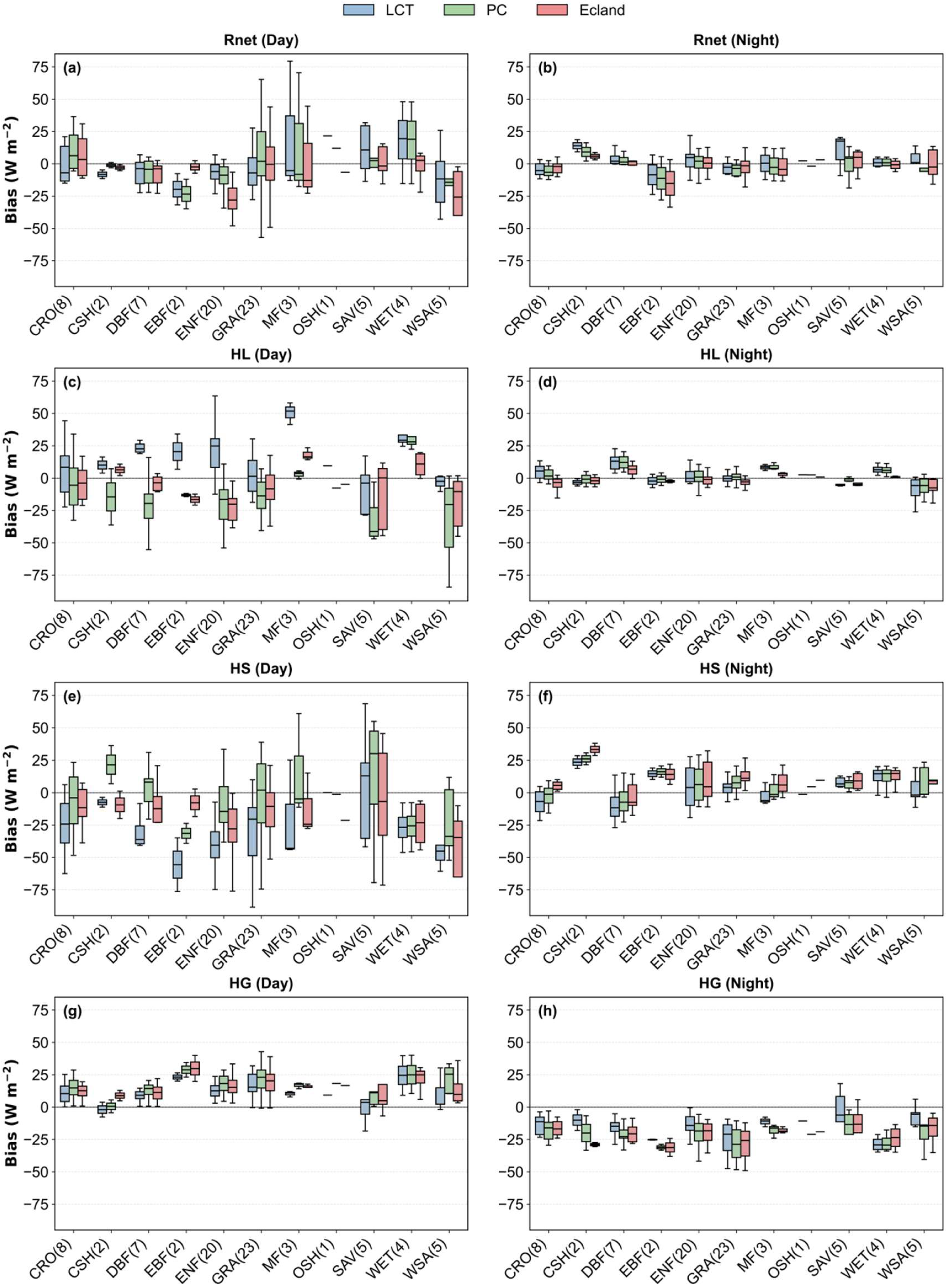
Figure 7.
Diurnal cycles of observed and simulated Rnet, HL, HS, and HG over four representative land cover types: deciduous broadleaf forest (DBF), evergreen needleleaf forest (ENF), grassland (GRA), and savanna (SAV).
Figure 7.
Diurnal cycles of observed and simulated Rnet, HL, HS, and HG over four representative land cover types: deciduous broadleaf forest (DBF), evergreen needleleaf forest (ENF), grassland (GRA), and savanna (SAV).
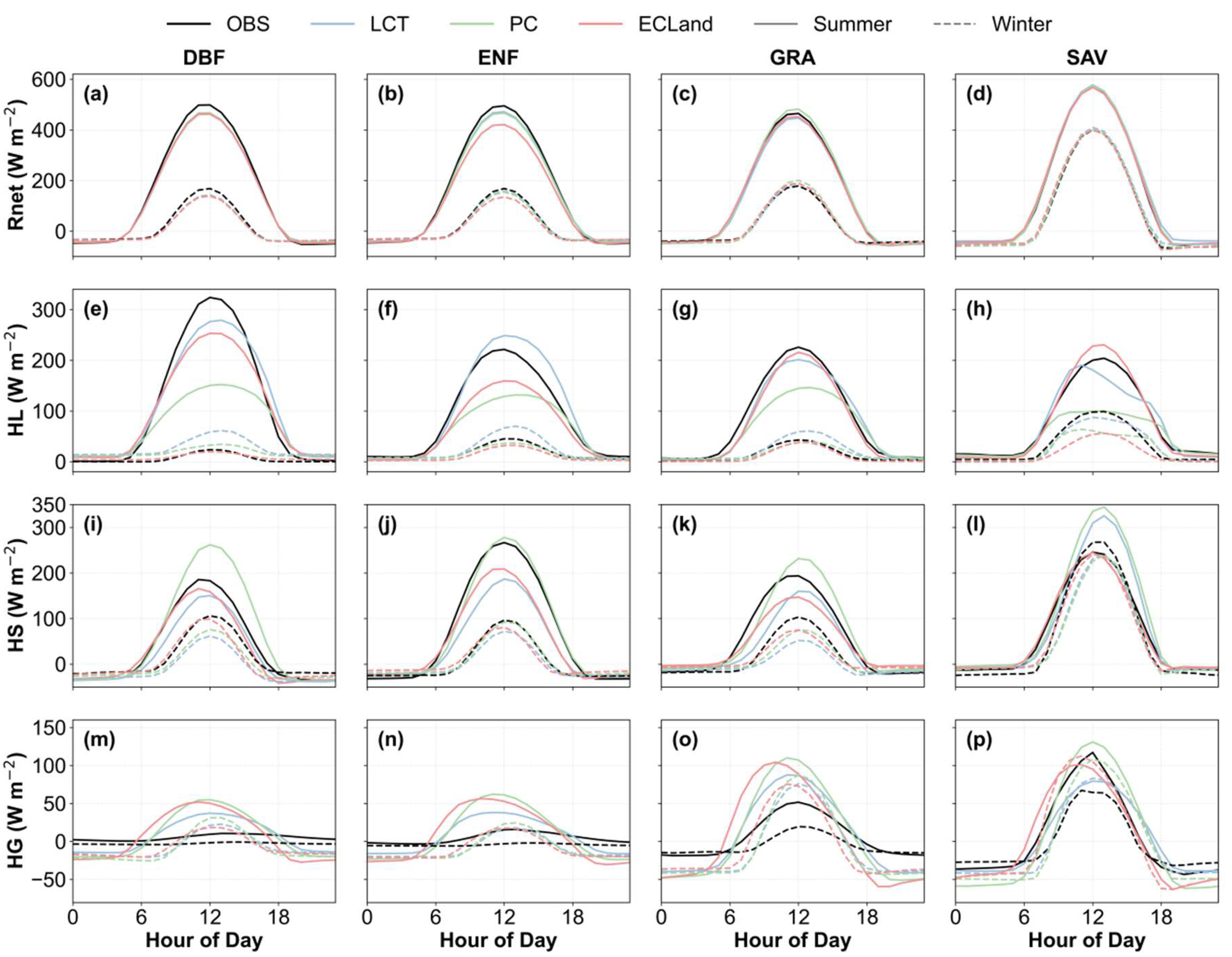
Figure 8.
Observed versus simulated annual cycles of surface (a) Rnet, (b) HL, (c) HS, and (d) HG across different land cover types and climate zones for the LCT, PC, and ECLand experiments.
Figure 8.
Observed versus simulated annual cycles of surface (a) Rnet, (b) HL, (c) HS, and (d) HG across different land cover types and climate zones for the LCT, PC, and ECLand experiments.
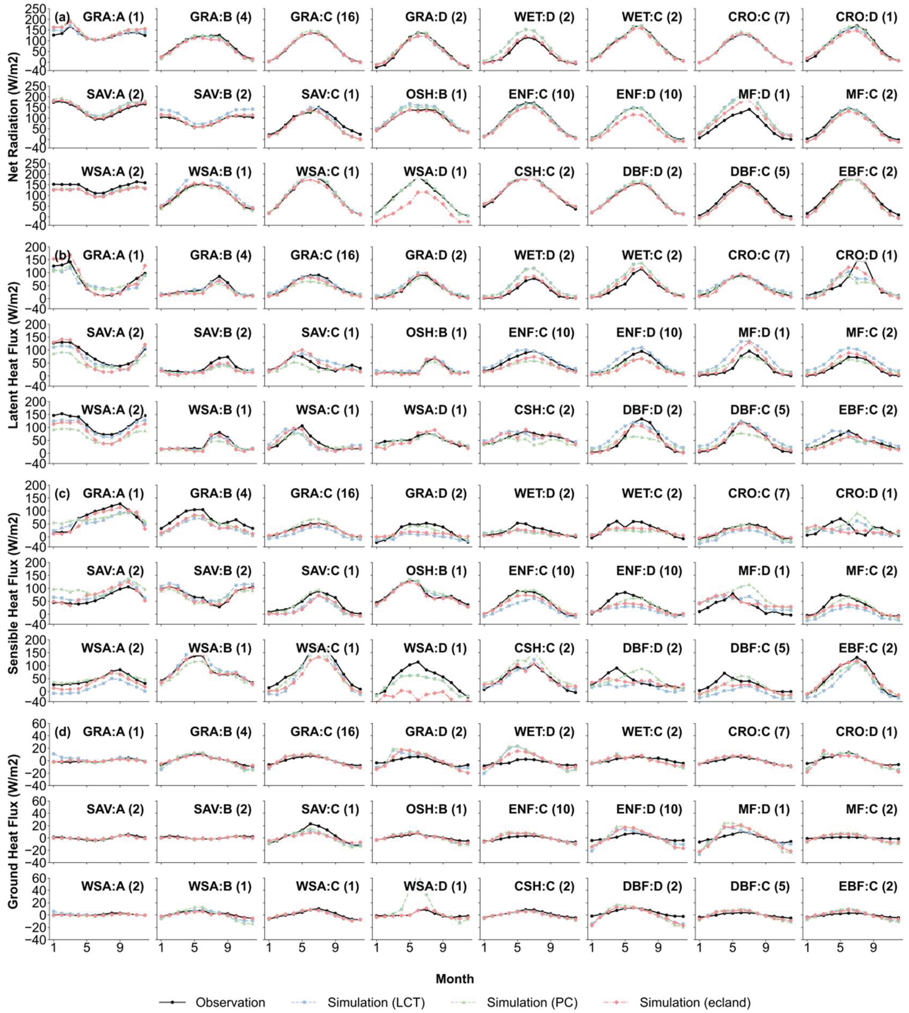

Table 1.
Modeling Experiments.
| Experiment | LSM | Forcing Data | Land Surface Characteristic Data |
| LCT | CoLM2024 | 80 sites from PLUMBER2 dataset | Shi et al. [49] |
| PC | CoLM2024 | 80 sites from PLUMBER2 dataset | Shi et al. [49] |
| ECLand | ECLand | 80 sites from PLUMBER2 dataset | Shi et al. [49]; ERA5 |
Table 2.
Definitions of evaluation metrics. Si and Oi denote simulated and observed values at time step i, respectively. S̄ and Ō represent their corresponding means, N is the total number of samples. Ŝi denotes the regression value based on ordinary least squares linear fitting (Ŝi = a + bOi), where a and b are the intercept and slope, respectively. Rsolar indicates concurrent downward shortwave radiation.
Table 2.
Definitions of evaluation metrics. Si and Oi denote simulated and observed values at time step i, respectively. S̄ and Ō represent their corresponding means, N is the total number of samples. Ŝi denotes the regression value based on ordinary least squares linear fitting (Ŝi = a + bOi), where a and b are the intercept and slope, respectively. Rsolar indicates concurrent downward shortwave radiation.
| Metrics | Definition | Metrics | Definition |
| R | RMSE | ||
| Nbias | RMSEs | ||
| IOA |
|
RMSEu |
Disclaimer/Publisher’s Note: The statements, opinions and data contained in all publications are solely those of the individual author(s) and contributor(s) and not of MDPI and/or the editor(s). MDPI and/or the editor(s) disclaim responsibility for any injury to people or property resulting from any ideas, methods, instructions or products referred to in the content. |
© 2026 by the authors. Licensee MDPI, Basel, Switzerland. This article is an open access article distributed under the terms and conditions of the Creative Commons Attribution (CC BY) license (http://creativecommons.org/licenses/by/4.0/).
Copyright: This open access article is published under a Creative Commons CC BY 4.0 license, which permit the free download, distribution, and reuse, provided that the author and preprint are cited in any reuse.


