
Submitted:
22 July 2026
Posted:
23 July 2026
You are already at the latest version
Abstract
We examine how restricting high-frequency trading (HFT) affects stock liquidity in China’s A-share market. Using China’s 2024 Provisions on Program Trading in the Securities Market as a quasi-natural experiment, we construct a stock-level high-frequency trading intensity index from tick-level order data and apply a difference-in-differences design. The regulation significantly improves liquidity by reducing bid-ask spreads and price impact. The effect is concentrated during stock price declines, suggesting that algorithmic traders withdraw liquidity when liquidity provision is most valuable. The improvement is stronger for small- and mid-cap stocks and margin-tradable stocks, which are more vulnerable to liquidity fragility. These findings show that targeted regulation of algorithmic trading can strengthen market resilience and investor protection in retail-dominated emerging markets.
Keywords:
algorithmic trading regulation
; high-frequency trading
; stock liquidity
; China’s A-share market
1. Introduction
Algorithmic trading has become an important feature of modern financial markets, but its implications for China’s A-share market remain unsettled. High-frequency trading (HFT), which relies on low-latency algorithms to submit, revise, and cancel orders at high speed has fundamentally transformed the market microstructure landscape. Whether HFT enhances or degrades market quality remains one of the central debates in financial economics (Biais et al., 2015; Menkveld, 2013; O’Hara, 2015). This question takes on particular significance in China’s A-share market, where institutional environments differ markedly from those of developed exchanges.
In this paper, we study the liquidity effects of restricting HFT in China’s A-share market. We exploit the introduction of the Provisions on Program Trading in the Securities Market (Trial), issued by the China Securities Regulatory Commission (CSRC) on May 11, 2024, as a quasi-natural experiment. This regulation imposes explicit constraints on HFT, including restrictions on order submission rates exceeding 300 per second or 20,000 per day. The exogenous nature of this policy shock, combined with cross-sectional variation in HFT exposure across stocks, allows us to implement a difference-in-differences (DID) framework for causal identification.
To identify heterogeneous exposure to the regulation, we construct a multidimensional HFT intensity index (HFTI) from tick-level order data. The index combines six order-level proxies: the order-to-trade ratio, cancellation frequency, trade frequency, order lifetime, best quote change frequency, and orders per shareholder. Stocks in the top 30% of the HFTI distribution are classified as more exposed to HFT and form the treatment group, whereas stocks in the bottom 30% form the control group. We then estimate a difference-in-differences model around the regulatory shock.
Our main findings are as follows. First, restricting HFT leads to a statistically and economically significant improvement in stock liquidity, as measured by both the Roll (1984) bid-ask spread and the Pastor & Stambaugh (2003) price impact measure. Second, the effect is strongly state-dependent: liquidity improvements are concentrated during periods of stock price decline, whereas no significant effect is detected during market rallies. This pattern is consistent with the view that HFT tends to withdraw liquidity precisely when it is most needed, amplifying fragility through procyclical order cancellations and momentum-driven selling (Kirilenko & Lo, 2013; Brogaard et al., 2014). Third, the liquidity benefits of HFT restrictions are disproportionately larger for small- and mid-cap stocks and for stocks eligible for margin trading, reflecting HFT’s preference for targets with thinner order books or greater leverage flexibility.
Our paper contributes to the literature along three dimensions. First, we provide causal evidence on the liquidity effects of HFT regulation from an emerging market context. While prior studies predominantly examine developed markets with deep liquidity pools and sophisticated investor bases (Hendershott et al., 2011; Brogaard et al., 2014; Menkveld & Zoican, 2017), evidence from markets with different institutional features remains limited. China offers a distinct institutional setting characterized by retail participation, a T+1 settlement rule, price limits, and the absence of formal market-making obligations for most stocks. These institutional features make China an informative setting for evaluating the effectiveness of HFT regulation.
Second, we develop a multidimensional HFT measurement approach that combines multiple order-level proxies into a composite index. This mitigates the well-known measurement error inherent in single-proxy approaches (Hasbrouck & Saar, 2013) and provides more reliable treatment assignment for the DID framework.
Third, beyond documenting average treatment effects, we provide new evidence on the state dependence of HFT’s liquidity effects. While the theoretical literature has long recognized the potential for HFT to exacerbate liquidity crises (Kirilenko & Lo, 2013; Biais et al., 2015), direct empirical evidence on how HFT restrictions affect liquidity during market stress remains scarce. Our finding that the benefits of HFT restrictions are concentrated during declining markets offers policy-relevant evidence that targeted regulation can serve as a stabilizing mechanism.
2. Literature Review and Research Hypothesis
The effect of HFT on market liquidity is a subject of active debate. Market microstructure theory suggests that liquidity fundamentally depends on the willingness of limit-order traders to provide depth, with its stability determined by information asymmetry and trader heterogeneity (Foucault et al., 2005; Li et al., 2021). Within this framework, HFT may either improve liquidity by reducing adverse selection costs or amplify fragility through procyclical trading behavior.
A substantial body of evidence documents the liquidity-enhancing role of HFT. By exploiting low-latency technology, high-frequency traders can rapidly update limit orders and increase depth near the best quotes, thereby narrowing bid–ask spreads (Hasbrouck and Saar, 2013; Boehmer et al., 2021). Ke and Zhang (2020) further show that HFT acts as a competitive liquidity supplier: by posting limit orders, high-frequency traders reduce spreads and lower execution costs for arbitrageurs. Algorithmic competition in limit-order placement also weakens the pricing power of traditional market makers and compresses trading costs (Hasbrouck and Saar, 2013; Jones, 2013). These studies suggest that, under normal market conditions, HFT can be an important source of market liquidity.
In contrast, a growing body of work highlights the procyclical and fragile nature of HFT-provided liquidity. Brogaard (2010) argues that high-frequency traders’ liquidity demand is primarily driven by short-lived arbitrage opportunities rather than long-term inventory motives, implying that HFT may consume rather than supply liquidity. Kirilenko and Lo (2013) further highlight the procyclical nature of HFT liquidity provision: high-frequency traders provide liquidity in tranquil markets, but their limited risk-bearing capacity and algorithmic herding can quickly turn them into liquidity demanders during market downturns. Consistent with this view, empirical evidence shows that, during extreme market conditions, high-frequency traders often cancel orders aggressively or trade in the direction of price movements, causing order-book depth to collapse and liquidity to dry up (Jain et al., 2016; Musciotto et al., 2021). Brogaard et al. (2017) also find that HFT can exploit liquidity suppliers through speed advantages and short selling, increasing adverse selection and widening bid-ask spreads.
These findings indicate that HFT’s role in liquidity is state-dependent. While generally enhancing liquidity in stable environments, it may exacerbate liquidity shortages in stressed conditions. This duality is particularly relevant for China’s retail-dominated A-share market, where shallow depth magnifies the impact of HFT withdrawals. The 2024 Provisions on Program Trading in the Securities Market (Trial) therefore provide a rare quasi-natural experiment to test whether restricting HFT can alleviate liquidity risks, especially during stocks decline periods.
Based on the theoretical and empirical literature reviewed above, we propose the following hypothesis:
Hypothesis. Algorithmic trading regulation improves stock liquidity in China’s A-share market, with a stronger effect during periods of stock price decline.
3. Research Design
3.1. Empirical Model
We employ a DID approach to identify the causal effect of restricting HFT on the stock liquidity. The baseline specification is:
where denotes stock liquidity measures. is the treatment indicator, which equals one if stock is classified into the treatment group and zero otherwise. Treatment group assignment is determined using tick-by-tick order data to identify stocks’ exposure to program trading. is the policy indicator, which equals one for May 2024 and onward, and zero otherwise. The captures the treatment effect of HFT restrictions on stock liquidity. The represents monthly time fixed effects. The denotes firm-quarter interactive fixed effects controlling for time-invariant firm characteristics and quarterly financial reporting effects. represents control variables including market capitalization, book-to-market ratio, price-earnings ratio, turnover, and volatility. Table 1 shows the definitions of these variables.
3.2. Dependent Variables
Measures of stock liquidity can generally be classified into two categories: bid-ask spread measures and market impact measures (Sarr & Lybek, 2002). Specifically, we employ the Roll_Spread to capture the bid-ask spread, and the Gamma measure to assess price impact.
The Roll_Spread measure, proposed by Roll (1984), is calculated as follows:
where represents the monthly spread measure calculated from daily price data, denotes the price change between day d and day d-1. This metric indirectly estimates the bid-ask spread by measuring the reversal in consecutive price changes. A higher Roll_Spread indicates greater transaction costs and poorer liquidity.
The Gamma measure, proposed by Pastor & Stambaugh (2003), is specified as:
where is the excess return of stock i on day d+1; is the stock’s return on day d; is the sign function that takes the value 1 for positive values, -1 for negative values, and 0 for zero; and represents trading volume. The coefficient captures the impact of stock returns and trading volume on day d on the excess return of day d+1. When liquidity is high, current trading volume has minimal impact on subsequent returns. Thus, the absolute value of , denoted as , is employed as a proxy for stock liquidity, where a larger value indicates poorer liquidity.
3.3. Data and Descriptive Statistics
We use A-share data from both the Shanghai and Shenzhen stock exchanges from January 2023 to May 2025. We exclude ST stocks and financial firms from our sample. The tick-by-tick data and minute-level price data are sourced from a Chinese securities firm. All other data are obtained from the CSMAR database. All variables are winsorized at the 1% and 99% levels to mitigate the influence of outliers. Table 2 reports the descriptive statistics.
3.4. Identification Strategy
Accurately identifying HFT remains challenging. A key contribution of our study is the construction of a multi-dimensional HFT index based on multiple measures, which can mitigate the measurement error inherent in single-proxy approaches.
3.4.1. Measurement Proxies
Proxy 1: Order-to-Trade Ratio. The order-to-trade ratio (OTR) is calculated as:
A higher OTR indicates a smaller proportion of orders resulting in trades, reflecting greater HFT influence.
Proxy 2: Cancellation Frequency. Cancellation frequency (CF), measured as the number of order cancellations within one-second intervals, is a key indicator of HFT behavior:
CF = Number of 1-second cancellations per day
The pattern of order cancellations within one second can sensitively reflect this dynamic adjustment behavior. Higher cancellation rates indicate more frequent strategic adjustments, demonstrating stronger HFT presence.
Proxy 3: Trade Frequency. Trade frequency (TF), measured as orders per minute, is calculated as:
With A-share trading hours from 9:30-11:30 and 13:00-15:00 (240 minutes total), this metric directly captures order submission intensity. HFT’s algorithmic decision-making generate exceptionally high order submission rates, making trade frequency a clear indicator of HFT participation intensity.
Proxy 4: Order Lifetime. Order lifetime (OL) measures the average duration from order submission to either execution or cancellation, calculated as:
HFT requires ultra-fast execution, typically resulting in extremely short order lifetimes. Smaller values of this metric better reflect the rapid entry and exit characteristics of HFT, making it a crucial identifier of HFT.
Proxy 5: Best Quote Change Frequency. Best quote change frequency (BQ) captures the number of changes per minute to the best bid or ask price, calculated as:
HFT exploits minute price discrepancies by frequently triggering changes to the best quotes. Higher values indicate more frequent quote updates, reflecting more intensive HFT.
Proxy 6: Orders per Shareholder. Orders per shareholder (OS) represent the ratio of daily order volume to the number of shareholders, calculated as:
Active HFT generates frequent order submissions, increasing this ratio. Generally, higher values indicate greater HFT influence on a stock, as algorithmic trading typically generates more orders relative to the shareholder base.
3.4.2. Standardization
To control for the confounding influence of firm size, we grouped A-share stocks from the Shanghai and Shenzhen exchanges (excluding financial and ST stocks). Specifically, we evenly divided the sample into five groups based on market capitalization, with each group containing 879 stocks.
Within each capitalization quintile, we standardize all six HFT proxies using the z-score method:
where represents the raw indicator value, denotes the group mean, and is the group standard deviation.
3.4.3. Calculate the High-Frequency Trading Index
We aggregate the six standardized proxies into the high frequency trading index (HFTI) using equal weights:
where ====1/6. Given the difficulty in distinguishing the relative importance of each proxy in capturing HFT, we adopt an equal-weighting approach. , , , , and represent the standardized values of the OTR, CF, TF, OL, BQ and OS. This composite index provides the basis for partitioning stocks into treatment and control groups.
3.4.4. Identification
We use tick-by-tick order data for A-share stocks on the Shanghai and Shenzhen exchanges from January 2023 to May 2024 as the basis for calculating the relevant indicators and the HFTI. Based on this dataset, we compute high-frequency trading metrics and derive each stock’s average HFTI through a weighted aggregation.
We then rank the sample stocks by HFTI, designating the top 30% as the treatment group and the bottom 30% as the control group. The former is more strongly affected by high-frequency trading and can better capture policy-induced changes, while the latter is less influenced and thus serves as a benchmark. This grouping provides a solid foundation for identifying the net effect of restricting high-frequency trading on stock liquidity.
4. Empirical Results
4.1. Baseline Results
Table 3 reports the estimated effects of restricting HFT on stock liquidity. Columns (1) and (2) use the bid-ask spread measure (Roll_Spread) as the dependent variable, while columns (3) and (4) use the price impact measure (Gamma). The treatment interaction term is consistently negative and statistically significant for both Roll_Spread and Gamma, indicating that restricting HFT significantly improves stock liquidity.
4.2. Parallel Trends Test
We use the following dynamic specification to conduct the parallel trends test:
where denotes event-time dummies, with representing the policy month.
Figure 1 presents the estimated coefficients with their 95% confidence intervals. The pre-treatment coefficients are insignificant, indicating no notable differences in stock liquidity between the HFT group and the non-HFT group before the policy. This confirms that the model satisfies the parallel trends assumption.
4.3. State-Dependent Effects
We next examine whether the policy effect depends on market states. If algorithmic trading regulation improves liquidity primarily by limiting procyclical liquidity withdrawal during stress, the effect should be concentrated during declining markets. To test this prediction, we partition the sample into declining-market observations (monthly stock return < 0) and rising-market observations (monthly stock return > 0) and re-estimate the baseline model within each subsample.
Table 4 presents the results. During periods of stock price decline, restricting HFT significantly reduces both bid-ask spreads and price impact. In contrast, the coefficients are statistically insignificant during market rallies. This asymmetry is consistent with the theoretical prediction that HFT amplifies liquidity fragility during stressed conditions through rapid position adjustments, massive order cancellations, and momentum-driven selling (Kirilenko & Lo, 2013). By constraining these procyclical behaviors, the regulation preserves market depth and mitigates liquidity dry-ups precisely when liquidity provision is most valuable.
4.4. Cross-Sectional Heterogeneity
4.4.1. Market Capitalization
If HFT disproportionately affects stocks with thinner order books, the benefits of restricting HFT should be more pronounced for smaller stocks. To test this, we partition stocks into large-cap (market cap ≥ ¥50 billion) and small- and mid-cap groups (market cap < ¥50 billion).
Table 5 confirms this prediction. HFT restrictions significantly reduce both bid-ask spreads and price impact for small- and mid-cap stocks, whereas the effects on large-cap stocks are statistically insignificant.
This divergence reflects fundamental differences in market depth. Smaller stocks typically exhibit lower market depth and higher price sensitivity, making their liquidity more vulnerable to external shocks and HFT. Consequently, they benefit more significantly from HFT restrictions. Table 6 further shows that these liquidity improvements for smaller stocks are concentrated during market declines, reinforcing the mechanism identified in Section 4.3.
4.4.2. Margin-Trading Eligibility
We further examine whether the policy effects vary by margin-trading eligibility. Chinese HFT frequently utilizes margin trading and short selling to implement short-term arbitrage strategies and to achieve de facto T+0 trading. These mechanisms provide greater leverage and flexibility, enabling HFT to exert stronger influence on market liquidity, particularly during downturns when momentum short selling through margin accounts may exacerbate liquidity evaporation.
Table 7 shows that HFT restrictions significantly improve liquidity for margin-tradable stocks, while the effects on non-margin-tradable stocks are insignificant. This heterogeneity reflects HFT’s strategic preference for stocks with greater leverage flexibility. Table 8 further confirms that the liquidity improvements for margin-tradable stocks are concentrated during market declines, consistent with the mechanism analysis.
5.5. Robustness Tests
4.5.1. Placebo Test
To ensure the robustness of our DID results, we conduct a placebo test following Li et al. (2016). This approach simulates a “false” scenario without actual policy impact by randomly assigning virtual treatment groups. Specifically, we perform 1,000 random samplings to construct placebo treatment groups and re-run our regression model. This random assignment ensures the virtual treatment groups are not based on actual HFT exposure, thus theoretically should not exhibit any genuine policy effect.
Figure 2 presents the placebo test results. The distribution of placebo coefficients clusters tightly around zero, and most placebo p-values exceed 0.10. The actual treatment coefficient lies well outside the placebo distribution, confirming that the baseline finding reflects a genuine policy effect rather than statistical artifact.
4.5.2. Alternative Liquidity Measures
Following Chung et al. (2020), Eaton et al. (2021), and Amihud (2002), we employ three alternative liquidity measures: the relative quoted spread (QSP), relative effective spread (ESP), and the Amihud illiquidity ratio (AMIHUD).
The relative quoted spread (QSP) is calculated as:
where represents the day d relative quoted spread , denotes the best ask price, indicates the best bid price, is the average of and , and represents the time interval between consecutive quotes. This time-weighted bid-ask spread better captures the price formation characteristics of China’s limit order market. Higher values of the relative quoted spread indicate greater transaction costs and poorer liquidity. After computing daily relative quoted spreads, we obtain monthly measures by calculating their averages.
The relative effective spread (ESP) is calculated as follows:
where is the transaction price. Higher ESP values indicate poorer liquidity. Daily ESP values are averaged to obtain monthly measures.
The Amihud illiquidity ratio (AMIHUD) is calculated as:
where represents the daily return and denotes the day d trading volume. This measure captures the price impact per unit of trading volume—higher values indicate poorer liquidity. After computing daily Amihud measures, we obtain monthly values by calculating their averages.
Table 9 presents regression results using these alternative measures. The policy is shown to significantly reduce all three indicators, indicating that restricting HFT significantly improves liquidity across all alternative measures, reinforcing the robustness of our main findings.
5. Conclusions
Whether algorithmic trading enhances or impairs market quality remains an important question in China’s financial market. This paper exploits the May 2024 Provisions on Program Trading in the Securities Market (Trial) issued by the CSRC as a quasi-natural experiment to examine how algorithmic trading regulation affects stock liquidity in China’s A-share market. Using tick-level order data, we construct a multidimensional HFT intensity index and implement a difference-in-differences design based on cross-sectional variation in stocks’ pre-policy exposure to HFT.
The central finding is that algorithmic trading regulation significantly improves stock liquidity. Treated stocks experience lower bid-ask spreads and lower price impact after the regulation, and the result is robust to placebo tests, alternative liquidity measures, and the inclusion of firm-quarter interactive fixed effects. These findings suggest that, in retail-dominated China’s A-share market, some forms of high-speed algorithmic trading may impose liquidity costs that are not fully captured by evidence from developed markets.
The results also reveal substantial state dependence. Liquidity improvements are concentrated during periods of stock price decline, whereas no significant effect is detected during market rallies. This asymmetric pattern is consistent with the theoretical prediction that HFT can amplify liquidity fragility during stress through procyclical order cancellations and momentum-driven trading. Regulation appears to mitigate these destabilizing behaviors and preserve liquidity when market resilience is most needed.
Cross-sectional analyses further show that the liquidity improvement is stronger for small- and mid-cap stocks and for margin-tradable stocks. These segments are more vulnerable to liquidity shocks because of thinner order books, higher price sensitivity, or greater leverage and short-selling flexibility. The evidence therefore supports a targeted regulatory approach that focuses on market segments where algorithmic trading may generate larger externalities.
The findings have implications for the policy debate on algorithmic trading in emerging markets. Evidence from developed markets often shows that HFT compresses spreads and reduces transaction costs under normal conditions. Our results do not contradict this view. Instead, they show that the net effect of HFT depends on institutional context and market state. In markets characterized by retail participation, T+1 settlement, price limits, and limited market-making obligations, targeted restrictions on HFT can improve liquidity and strengthen market resilience without eliminating the broader informational role of algorithmic trading.
Author Contributions
Conceptualization, J.W.; methodology, L.J.; software, S.C.; validation, J.W., L.J. and S.C.; formal analysis, L.J.; investigation, J.W.; resources, J.W.; data curation, S.C.; writing—original draft preparation, J.W.; writing—review and editing, L.J.; visualization, S.C.; supervision, L.J.; project administration, L.J.; funding acquisition, J.W. All authors have read and agreed to the published version of the manuscript.
Funding
This research received no external funding.
Institutional Review Board Statement
Not applicable.
Informed Consent Statement
Not applicable.
Data availability statement
The tick-level order data used in this study were obtained from a Chinese securities firm under license and are not publicly available. Other firm-level and market variables were obtained from CSMAR. Data may be available from the corresponding author upon reasonable request and with permission from the data providers.
Acknowledgments
During the preparation of this manuscript/study, the authors used ChatGPT (OpenAI, GPT-5.5 Thinking) for language polishing and improving the clarity and readability of academic expressions. The authors have reviewed and edited the output and take full responsibility for the content of this publication.
Conflicts of Interest
Author Shaobin Chen is employed by the company Zhejiang Zheshang Financial Holdings Co., Ltd. The authors declare that the research was conducted in the absence of any commercial or financial relationships that could be construed as a potential conflict of interest.
References
- Amihud, Y. (2002). Illiquidity and stock returns: cross-section and time-series effects. Journal of financial markets, 5(1), 31-56. [CrossRef]
- Biais, B., Foucault, T., & Moinas, S. (2015). Equilibrium fast trading. Journal of Financial economics, 116(2), 292-313. [CrossRef]
- Boehmer, E., Fong, K., & Wu, J. J. (2021). Algorithmic trading and market quality: International evidence. Journal of Financial and Quantitative Analysis, 56(8), 2659-2688. [CrossRef]
- Brogaard, J. (2010). High frequency trading and its impact on market quality. Northwestern University Kellogg School of Management Working Paper, 66(10).
- Brogaard, J., Carrion, A., Moyaert, T., Riordan, R., Shkilko, A., & Sokolov, K. (2018). High frequency trading and extreme price movements. Journal of Financial Economics, 128(2), 253-265. [CrossRef]
- Brogaard, J., Hendershott, T., & Riordan, R. (2014). High-frequency trading and price discovery. The Review of Financial Studies, 27(8), 2267-2306. [CrossRef]
- Brogaard, J., Hendershott, T., & Riordan, R. (2017). High frequency trading and the 2008 short-sale ban. Journal of Financial Economics, 124(1), 22-42. [CrossRef]
- Chung, K. H., Lee, A. J., & Rösch, D. (2020). Tick size, liquidity for small and large orders, and price informativeness: Evidence from the Tick Size Pilot Program. Journal of Financial Economics, 136(3), 879-899. [CrossRef]
- Eaton, G. W., Irvine, P. J., & Liu, T. (2021). Measuring institutional trading costs and the implications for finance research: The case of tick size reductions. Journal of Financial Economics, 139(3), 832-851. [CrossRef]
- Foucault, T., Kadan, O., & Kandel, E. (2005). Limit order book as a market for liquidity. The Review of Financial Studies, 18(4), 1171-1217. [CrossRef]
- Hasbrouck, J., & Saar, G. (2013). Low-latency trading. Journal of Financial Markets, 16(4), 646-679. [CrossRef]
- Hendershott, T., Jones, C. M., & Menkveld, A. J. (2011). Does algorithmic trading improve liquidity?. The Journal of finance, 66(1), 1-33. [CrossRef]
- Jain, P. K., Jain, P., & McInish, T. H. (2016). Does high-frequency trading increase systemic risk?. Journal of Financial Markets, 31, 1-24.
- Jones, C. M. (2013). What do we know about high-frequency trading?. Columbia Business School Research Paper, (13-11).
- Ke, Y., & Zhang, Y. (2020). Does high-frequency trading reduce market underreaction to earnings news?. Finance Research Letters, 34, 101239. [CrossRef]
- Kirilenko, A. A., & Lo, A. W. (2013). Moore’s law versus murphy’s law: Algorithmic trading and its discontents. Journal of Economic Perspectives, 27(2), 51-72.
- Li, P., Lu, Y., & Wang, J. (2016). Does flattening government improve economic performance? Evidence from China. Journal of Development Economics, 123, 18-37. [CrossRef]
- Li, S., Wang, X., & Ye, M. (2021). Who provides liquidity, and when?. Journal of Financial economics, 141(3), 968-980.
- Menkveld, A. J. (2013). High frequency trading and the new market makers. Journal of financial Markets, 16(4), 712-740. [CrossRef]
- Menkveld, A. J., & Zoican, M. A. (2017). Need for speed? Exchange latency and liquidity. The Review of Financial Studies, 30(4), 1188-1228. [CrossRef]
- Musciotto, F., Piilo, J., & Mantegna, R. N. (2021). High-frequency trading and networked markets. Proceedings of the National Academy of Sciences, 118(26), e2015573118. [CrossRef]
- O’hara, M. (2015). High frequency market microstructure. Journal of financial economics, 116(2), 257-270. [CrossRef]
- Pastor, L., & Stambaugh, R. F. (2003). Liquidity risk and expected stock returns. Journal of Political Economy, 111(3), 642-685. [CrossRef]
- Roll, R. (1984). A simple implicit measure of the effective bid-ask spread in an efficient market. The Journal of Finance, 39(4), 1127-1139. [CrossRef]
- Sarr, A., & Lybek, T. (2002). Measuring liquidity in financial markets. IMF Working Paper No. 02/232. [CrossRef]
Figure 1.
Parallel trends test. This figure plots the estimated coefficients from the dynamic DID specification, with 95% confidence intervals. The pre-treatment coefficients are statistically insignificant, confirming the parallel trends assumption.
Figure 1.
Parallel trends test. This figure plots the estimated coefficients from the dynamic DID specification, with 95% confidence intervals. The pre-treatment coefficients are statistically insignificant, confirming the parallel trends assumption.
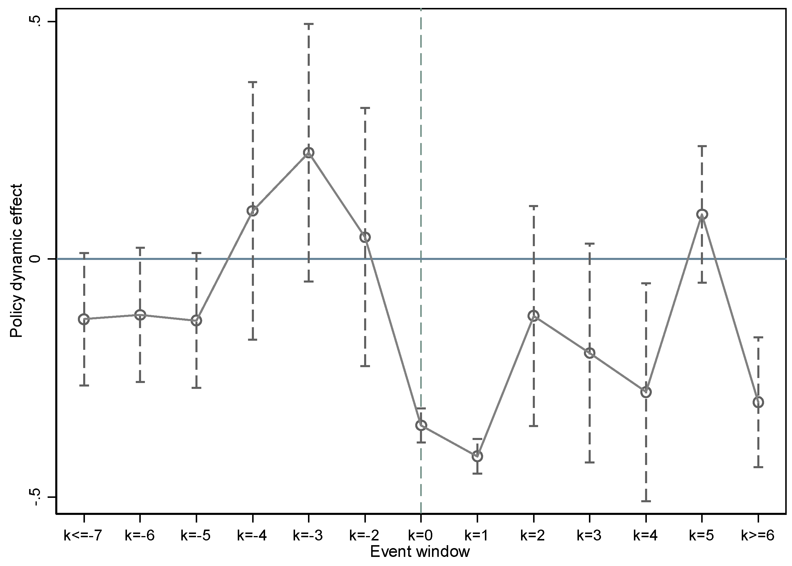
Figure 2.
Placebo test for stock liquidity. This figure displays the distribution of coefficients from 1,000 placebo regressions. The dependent variable is Roll_Spread. The vertical solid line indicates the mean placebo coefficient, and the dashed horizontal line marks the p = 0.10 threshold.
Figure 2.
Placebo test for stock liquidity. This figure displays the distribution of coefficients from 1,000 placebo regressions. The dependent variable is Roll_Spread. The vertical solid line indicates the mean placebo coefficient, and the dashed horizontal line marks the p = 0.10 threshold.
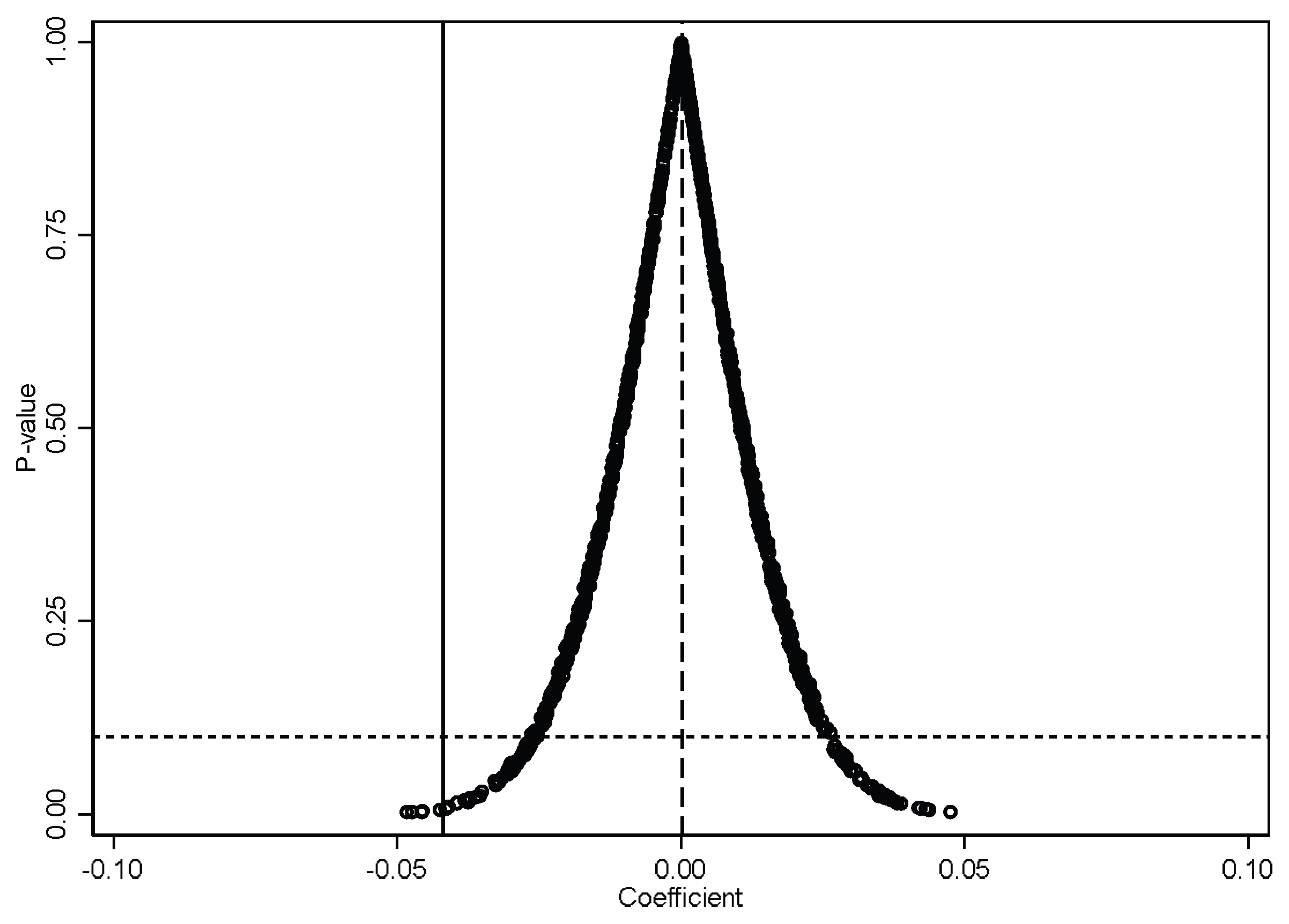

Table 1.
Variable definitions.
| Variable | Definition | Measurement |
| Treat | Treatment indicator | Equals 1 if the stock belongs to treatment group, and zero otherwise |
| Post | Policy indicator | Equals 1 for periods after policy announcement, and zero otherwise |
| MV | Market capitalization | Natural logarithm of market capitalization |
| BP | Book-to-market ratio | Book value / Market value |
| PE | Price-to-earnings ratio | Stock price / Earnings per share |
| TR | Turnover ratio | Trading volume / Shares outstanding |
| Volatility | Return volatility | Standard deviation of daily returns within the month |
Table 2.
Descriptive statistics.
| Variables | Obs | Mean | SD | Min | Median | Max |
| Roll_Spread | 73855 | 0.252 | 0.488 | 0 | 0.053 | 2.906 |
| Gamma | 73855 | 0.818 | 1.145 | 0.005 | 0.405 | 6.723 |
| MV | 73850 | 4.004 | 1.107 | 1.892 | 3.854 | 7.362 |
| BP | 73850 | 0.523 | 0.349 | 0.059 | 0.433 | 1.847 |
| PE | 73850 | 29.71 | 143.8 | -665 | 24.59 | 761 |
| TR | 73850 | 3.009 | 3.348 | 0.228 | 1.802 | 18.47 |
| Volatility | 73850 | 0.028 | 0.015 | 0.007 | 0.025 | 0.076 |
Table 3.
The impact of restricting high-frequency trading on stock liquidity.
| Roll_Spread (1) | Roll_Spread (2) | Gamma (3) | Gamma (4) | |
| Treat × Post | -0.042*** | -0.042*** | -0.102* | -0.131** |
| (0.015) | (0.016) | (0.052) | (0.052) | |
| TR | 0.001 | 0.022*** | ||
| (0.002) | (0.003) | |||
| MV | -0.052*** | -0.239*** | ||
| (0.020) | (0.042) | |||
| BP | -0.091*** | -0.586*** | ||
| (0.035) | (0.098) | |||
| PE | -0.000 | -0.000 | ||
| (0.000) | (0.000) | |||
| Volatility | 0.135 | -10.771*** | ||
| (0.328) | (0.641) | |||
| Constant | 0.262*** | 0.514*** | 0.842*** | 2.349*** |
| (0.004) | (0.084) | (0.013) | (0.196) | |
| Month FE | Yes | Yes | Yes | Yes |
| Firm × Quarter FE | Yes | Yes | Yes | Yes |
| N | 73851 | 73841 | 73851 | 73841 |
| Adj. R² | 0.378 | 0.378 | 0.423 | 0.428 |
Standard errors in parentheses, * p < 0.1, ** p < 0.05, *** p < 0.01.
Table 4.
Policy effects on liquidity during market declines and rallies.
| Roll_Spread | Gamma | |||
| Treat × Post | -0.051*** | -0.036 | -0.315*** | 0.111 |
| (0.019) | (0.047) | (0.087) | (0.092) | |
| Controls | All | All | All | All |
| Month FE | Yes | Yes | Yes | Yes |
| Firm × Quarter FE | Yes | Yes | Yes | Yes |
| N | 28269 | 22705 | 28269 | 22705 |
| Adj. R² | 0.402 | 0.347 | 0.470 | 0.395 |
Standard errors in parentheses, * p < 0.1, ** p < 0.05, *** p < 0.01.
Table 5.
Policy effects by market capitalization.
| Roll_Spread | Gamma | |||
| Small- and mid-cap | Large-cap | Small- and mid-cap | Large-cap | |
| Treat × Post | -0.038** | -0.143 | -0.134** | -0.040** |
| (0.015) | (0.094) | (0.054) | (0.020) | |
| Controls | All | All | All | All |
| Month FE | Yes | Yes | Yes | Yes |
| Firm × Quarter FE | Yes | Yes | Yes | Yes |
| N | 70509 | 3332 | 70509 | 3332 |
| Adj. R² | 0.378 | 0.363 | 0.418 | 0.401 |
Standard errors in parentheses, * p < 0.1, ** p < 0.05, *** p < 0.01.
Table 6.
Policy effects on small- and mid-cap stock liquidity during market declines and rallies.
| Small- and mid-cap & Return<0 | Small- and mid-cap & Return>0 | |||
| Roll_Spread | Gamma | Roll_Spread | Gamma | |
| Treat × Post | -0.054*** | -0.320*** | 0.001 | 0.117 |
| (0.019) | (0.088) | (0.046) | (0.099) | |
| Controls | All | All | All | All |
| Month FE | Yes | Yes | Yes | Yes |
| Firm × Quarter FE | Yes | Yes | Yes | Yes |
| N | 26905 | 26905 | 21732 | 21732 |
| Adj. R² | 0.397 | 0.460 | 0.354 | 0.385 |
Standard errors in parentheses, * p < 0.1, ** p < 0.05, *** p < 0.01.
Table 7.
Policy effects by margin-trading eligibility.
| Roll_Spread | Gamma | |||
| margin-tradable | non- margin-tradable |
margin-tradable | non- margin-tradable |
|
| Treat × Post | -0.061*** | -0.020 | -0.110* | -0.187 |
| (0.021) | (0.022) | (0.058) | (0.119) | |
| Controls | All | All | All | All |
| Month FE | Yes | Yes | Yes | Yes |
| Firm × Quarter FE | Yes | Yes | Yes | Yes |
| N | 51335 | 22506 | 51335 | 22506 |
| Adj. R² | 0.385 | 0.322 | 0.475 | 0.326 |
Standard errors in parentheses, * p < 0.1, ** p < 0.05, *** p < 0.01.
Table 8.
Policy effects on margin-tradable stock liquidity during market declines and rallies.
| margin-tradable & Return<0 | margin-tradable & Return>0 | |||
| Roll_Spread | Gamma | Roll_Spread | Gamma | |
| Treat × Post | -0.075*** | -0.272*** | -0.073 | 0.271 |
| (0.027) | (0.100) | (0.063) | (0.266) | |
| Controls | All | All | All | All |
| Month FE | Yes | Yes | Yes | Yes |
| Firm × Quarter FE | Yes | Yes | Yes | Yes |
| N | 20333 | 20333 | 15140 | 7501 |
| Adj. R² | 0.409 | 0.520 | 0.347 | 0.308 |
Standard errors in parentheses, * p < 0.1, ** p < 0.05, *** p < 0.01.
Table 9.
Regression results with alternative dependent variables.
| QSP | ESP | AMIHUD | |
| Treat × Post | -3.816*** | -7.658*** | -0.326*** |
| (0.701) | (1.517) | (0.070) | |
| Controls | All | All | All |
| Month FE | Yes | Yes | Yes |
| Firm × Quarter FE | Yes | Yes | Yes |
| N | 73841 | 73841 | 73841 |
| Adj. R² | 0.966 | 0.953 | 0.867 |
Standard errors in parentheses, * p < 0.1, ** p < 0.05, *** p < 0.01.
Disclaimer/Publisher’s Note: The statements, opinions and data contained in all publications are solely those of the individual author(s) and contributor(s) and not of MDPI and/or the editor(s). MDPI and/or the editor(s) disclaim responsibility for any injury to people or property resulting from any ideas, methods, instructions or products referred to in the content. |
© 2026 by the authors. Licensee MDPI, Basel, Switzerland. This article is an open access article distributed under the terms and conditions of the Creative Commons Attribution (CC BY) license (http://creativecommons.org/licenses/by/4.0/).
Copyright: This open access article is published under a Creative Commons CC BY 4.0 license, which permit the free download, distribution, and reuse, provided that the author and preprint are cited in any reuse.


