
Submitted:
21 July 2026
Posted:
23 July 2026
You are already at the latest version
Abstract
The widespread adoption of autonomous vehicle technologies requires accurate predictions of coordinated multi-agent motion. While predicting such motion under arbitrary control mechanisms is generally intractable, we focus on certain classes of optimal control where the system dynamics reduce to Lie-Poisson equations. In this context, we aim to learn the dynamics solely from data, without prior knowledge of the control Hamiltonian or the inter-agent interaction laws. To achieve this, we introduce Control Optimal Lie-Poisson Neural Networks (CO-LPNets), built from a composition of Poisson maps. By design, CO-LPNets preserve the system’s Casimir invariants to machine precision. We demonstrate the completeness of these neural networks and highlight their representational efficiency. We apply CO-LPNets to systems of interacting particles on the SO(3) and SE(3) Lie groups, modeling coupled rigid body rotations and the spatial navigation of unmanned vehicles, respectively. Numerical evaluations confirm that CO-LPNets accurately learn the global phase-space dynamics from sparse data, faithfully reproducing trajectories over hundreds of time steps. Furthermore, we demonstrate the robustness of the architecture against observational noise. Requiring minimal training data (∼200 points per dimension) and highly compact architectures (∼1000 parameters), CO-LPNets offer a highly efficient, structure-preserving solution well-suited for practical edge deployment in autonomous systems.
Keywords:
data-based modeling
; Poisson systems
; Casimir conservation
; symmetry reduction
1. Problem Setup and General Approach
Understanding and predicting the collective motion of interacting unmanned vehicles is becoming increasingly important for civilian and military uses. Mathematically, the problem we consider can be formulated as follows. Suppose we observe the evolution of a system of N interacting elements, each of them evolving in its own phase space. For the unmanned aerial vehicles (UAVs) or underwater drones, the phase space of the individual particle is the Lie group , where is the group of rotations and translations in three-dimensional space. For land-based drones or drones operating on the sea surface, the phase space is also the Lie group . This, in general, practical applications of unmanned vehicles are occurring on some Lie group G. Suppose that we have observations of each particle of the system, and we know that the objects are connected and controlled, but we have limited information about the actual control procedure and the connection between them. The goal is to predict the collective motion of the system from data, without the need to decipher the actual information about the method of control.
In its most general formulation, without any information about the control, the prediction of motion is likely impossible. However, with some limited assumptions on the nature of control, a solution to this problem can be found. In what follows, we assume that the collective behavior comes from the optimal control procedure. The process of symmetry reduction of problems of collective behavior using optimal control was developed in Justh and Krishnaprasad [1,2]. These papers show that the control Hamiltonians are of the type allowing complete reduction to coupled Lie-Poisson systems. We are going to predict the motion in exactly that case of complete Lie-Poisson reduction as described in [1,2]. Without any knowledge of the system, the actual control Hamiltonian, depending on the directions of control and the control amplitudes, cannot be recovered completely. However, we show that instead of learning the Hamiltonian and the nature of control, we can recreate phase space trajectories and predict dynamics of the system in the future, based on the available data observations only, for an arbitrary control Hamiltonian. In order to do that, we propose a new type of Neural Networks, which we call CO-LPNets (Control Optimal Lie–Poisson Neural Networks), which are a generalization of Lie-Poisson Neural Networks [3] for the problems of optimal control of multiple interacting vehicles.
Data-Driven Discovery of Differential Equations with Structure
Recent advancements in scientific machine learning focus heavily on identifying the governing dynamics of physical systems from observational data. For autonomous systems evolving on a state space manifold, this typically involves reconstructing the underlying phase flow from a discrete sequence of observed states .
While generic, unconstrained neural networks excel at interpolating data, they frequently fail in engineering and physics applications where long-term stability hinges on respecting known conservation laws. To address this, frameworks like Physics-Informed Neural Networks (PINNs) [4,5] introduce physical boundaries and structural residuals directly into the loss function. However, because PINNs rely on optimization-based soft constraints, they regularly exhibit optimization failures, spectral bias, and severe error accumulation when applied to highly structured geometric systems, such as canonical Hamiltonian or Lie–Poisson dynamics [6]. For these systems, minor violations of the underlying geometry accumulate over time, destroying the qualitative correctness of long-term trajectories. Consequently, our work shifts the focus from soft-penalty architectures to exact, structure-preserving data-driven representations.
Continuous vs. Discrete Geometric Learning paradigms
Data-driven geometric computing generally splits into two distinct methodological paradigms based on how time is treated:
- Continuous Operator Learning: This paradigm aims to learn the continuous-time vector field or infinitesimal flow of the dynamics, modeling the governing operator as . In structured settings, e.g., describing a Hamiltonian system, approaches like Hamiltonian Neural Networks (HNNs) [7] parameterize the vector field via a learned Hamiltonian function. While effective, a significant drawback of this approach is that generating actual trajectories requires pairing the learned model with an external, secondary numerical scheme (e.g., a structure-preserving integrator [8]). Any discretization error introduced by this secondary solver can still degrade the physical invariants.
- Discrete Flow-Map Learning: Rather than approximating the continuous vector field, this paradigm directly learns the discrete-time flow map over a fixed time step h. Trajectories are generated strictly through recursive map composition: . This architecture inherently bypasses the need for an external ODE solver. Existing literature has successfully leveraged this framework for canonical systems via SympNets [9] and extended it to non-canonical Poisson spaces [3,10,11,12,13].
The methodology developed in this paper uses the discrete data-driven computing paradigm. In other words, we learn discrete mappings and not the Hamiltonian.
By directly identifying the discrete flow map on the reduced space , our framework eliminates the accumulation of artificial dissipation typical of continuous-operator approximations. As detailed in the subsequent sections, embedding the Lie–Poisson geometry directly into the network architecture allows our model to preserve non-canonical invariant quantities—specifically, Casimir functions—to machine precision indefinitely, ensuring long-term bounded energy errors and stable rollout trajectories even within chaotic regimes.
2. Literature Review
2.1. Data-Based, Structure-Preserving Computing of Poisson Systems
2.1.1. Continuous Systems with Structure
Since the focus of this paper is the data-based computing of control-Hamiltonian systems, we present a short review of the recent progress in that field.
Various methodologies exist for applying physics-informed data techniques to Hamiltonian systems while respecting their intrinsic mathematical architecture. Much of the existing literature focuses on canonical Hamiltonian systems, where the state vector is -dimensional, composed of coordinates and momenta ; thus, . In these cases, the evolution equation is governed by a Hamiltonian function , such that the operator takes the form:
where represents the identity matrix. If we take an arbitrary smooth function , its’ time evolution along a trajectory of (1) is defined by the canonical Poisson bracket:
This bracket acts as a mapping that transforms two smooth functions into another smooth function of the same variables. Mathematically, it is a bilinear, antisymmetric operator acting on differentiable function, which, satisfies the Leibniz rule (acting as a derivative), and fulfills the Jacobi identity:
for all smooth functions . Brackets that possess these four properties but differ from the form in (2) are categorized as general or non-canonical Poisson brackets. The resulting equations of motion are called Hamiltonian (usually for canonical brackets) or Poisson systems, for non-canonical Hamiltonian brackets. The non-canonical systems frequently possess a non-trivial null space, leading to the preservation of specific quantities known as Casimir invariants (or Casimirs). These invariants are structural features of the Poisson bracket itself, remaining constant regardless of the specific Hamiltonian chosen. This proposal concentrates on data-driven computational strategies for a significant class of these non-canonical Poisson systems.
One prominent research direction focuses on extracting the system’s Hamiltonian or its underlying Poisson bracket directly from observed data. This approach was pioneered for canonical systems by Hamiltonian Neural Networks (HNN) [7], which approximate by fitting the observed state evolution through the relations in (1). This approach, respecting the structure of the equations, allows for more robust and accurate trajectory approximations than standard neural networks. This approach has been further refined to handle chaotic transitions and adaptive parameter learning [14], with theoretical foundations for the existence of such learned Hamiltonians established in [15].
An alternative strategy is found in Lagrangian Neural Networks (LNNs) [16], which model the Euler-Lagrange equations in the coordinate-velocity space, bypassing the need for a Legendre transform to coordinates. More recently, learning vector fields for non-canonical Poisson brackets was explored in [17], though enforcing the Jacobi identity (3) remains a significant hurdle. Furthermore, recent work [18] utilized kernel ridge regression to learn Hamiltonians from noisy data in Poisson systems. While these methods can accurately reconstruct vector fields, isolating the true Hamiltonian is challenging because it is defined only up to the addition of an arbitrary function of the Casimirs, whereas the ML methods would try to find a particular Hamiltonian.
Crucially, these “continuous” methods assume that once the vector field is learned, it can be solved using standard numerical integration. However, simulating Hamiltonian systems, especially over long time scales, requires caution, as generic solvers are not structure-preserving and thus, for example, violate conservation laws for energy and momenta. To maintain physical validity in long-term simulations, one must employ variational integrators [8,19,20]. While these specialized methods preserve momentum-like quantities to machine precision, they are often significantly more computationally demanding than their non-structure-preserving counterparts.
2.1.2. Discrete Mapping Approach
We utilize a different strategy, namely, determining the phase space transformations that satisfy specific structural properties. For canonical Hamiltonian dynamics, a fundamental theorem by Poincaré asserts that the flow of the system (1)—which maps initial conditions to a state at time t—is a symplectic transformation [21,22,23]. Formally, for a state , the flow must satisfy:
Rather than identifying the governing equations and subsequently integrating them, several researchers have proposed learning these symplectic mappings directly from empirical data.
Early developments in such learning of such symplectic transformations started with Symplectic Recurring Neural Networks (SRNNs) [24], which approximate transformations using discretized symplectic numerical schemes. That work determined that enforcing canonical structures significantly improves robustness when dealing with noisy datasets. Similarly, Non-Separable Symplectic Neural Networks (NSSNNs) were introduced in [25] to approximate symplectic steps for non-separable Hamiltonians, utilizing the explicit integrator proposed in [26]. From a Lagrangian perspective, [27] explored mappings in the phase space through structure-preserving discretization, a framework we have recently extended to encompass dissipative forces and thermodynamic systems [28].
Further advancements in learning symplectic maps were achieved through three distinct methodologies [9,29]. The first, SympNets [9], constructs dynamics by composing specific types of symplectic layers. In contrast, Generating Function Neural Networks (GFNNs) [29] derive mappings via a generating function approach, allowing for explicit long-term error estimation. Additionally, [30] introduced HénonNets, which utilize Hénon mappings to learn Poincaré maps while maintaining symplectic integrity. These architectures have successfully simulated the long-term behavior of integrable systems, e.g., pendulums and planetary orbits, and chaotic regimes like the three-body problem, demonstrating the potential of direct transformation learning.
The SympNet framework was adapted for non-canonical Poisson systems in [10] under the name Poisson Neural Networks (PNNs). By invoking the Lie-Darboux theorem, PNNs transform non-canonical coordinates into local canonical ones, assuming a constant-rank Poisson structure. However, this approach faces two major hurdles: the Lie-Darboux transformation is usually (and for most cases) local rather than global, and the model fails to preserve Casimirs exactly. However, Casimir preservation is essential for the reliability of long-term ensemble simulations [31], so we will be interested in methods that preserve Casimirs with machine precision.
An alternative route suggested in [12] involves solving approximate Hamilton-Jacobi equations for symmetry-reduced systems. This allows for the construction of transformations that exactly conserve momentum maps and Casimirs; however, solving the Hamilton-Jacobi equations for general, complex systems remains computationally and analytically prohibitive. More recently, [32] introduced LocSympNets and their symmetric counterparts, SymLocSympNets, which rely on the composition of volume-preserving mappings. These models have shown high accuracy in long-term simulations of rigid body dynamics, linear advection, and particles in magnetic fields. While these methods are highly effective for Poisson-like problems, their broader application has been limited because the mathematical completeness of their proposed activation matrices remains unproven.
2.2. Optimal Control via Neural Networks
Because of the importance of the problem of optimal control in engineering, and flexibility of neural networks, optimal control via neural networks remains an active area of research. For example, [33] introduces the equations of motion in Pontryagin’s principle as a soft constraint, in the framework similar to what that later becomes known as PINNs. The authors of [34] used the input convex neural networks for control tractability. Applications of neural networks to problems such as robotics manipulation [35] and landing problems in aeronautics [36] were considered. For a recent survey of applications of neural networks in optimal control problems we refer the reader to a recent review [37]. While the progress achieved has been substantial, these methods have not used the advances in structure-preserving networks to fully utilize the mathematical structure inherent to Pontryagin’s principle. However, preservation of the structure of the equations in neural networks is essential for reproducing accurate long-term dynamics [3,9], which is exactly the point of our paper.
2.3. Data-Based Predictions for Lie-Poisson Systems
As discussed in more details in Section 4, the problem of optimal control for coupled autonomous systems naturally adopts the Lie-Poisson structure characteristic of many physical systems. Drawing on the work of [1,2], symmetry reduction of controlled Hamiltonian systems results in a complete Lie-Poisson reduction to the direct product of individual Lie algebras, representing the reduced phase space for each vehicle. The symmetry reduction for multi-particle systems is often incomplete, requiring the tracking of relative Lie group elements in addition to motion on the Lie algebra [38]. However, such complexity is bypassed in Lie-Poisson optimal control due to the specific functional form of the Hamiltonian [1,2].
In Lie-Poisson systems, the Poisson bracket is known a priori, as its’ explicit form is derived directly from the underlying Lie algebra commutator. Selecting the specific Hamiltonian is a subsequent task dictated by the physics or control objectives of the problem. To facilitate data-driven computing within this framework, [3,13] developed methods to construct activation maps directly from these brackets. These methods predict dynamics using maps generated by explicit solutions of specific Lie-Poisson systems. As demonstrated in [3], this approach is universally applicable to finite-dimensional Lie-Poisson systems and any Poisson system where explicit integration of the governing equations for suitable transformations is feasible.
The computational advantage of using explicit integration in Lie-Poisson equations to accelerate time-stepping was initially identified in [39], though its application was restricted to specific forms of the Hamiltonian. The methodology we develop in this article, by contrast, accommodates arbitrary Hamiltonians. In fact, the Hamiltonian does not need to be specified to construct the Neural Network; we only require knowledge of the underlying symmetry and the corresponding Lie-Poisson bracket. This is a robust assumption, as symmetries and brackets are fundamental to the problem’s geometric formulation and are known exactly. In contrast, the Hamiltonian is often a modeling choice that may only be known approximately [40].
In Lie-Poisson systems, the configuration manifold is defined on a Lie group G. For a group-invariant system, the dynamics can be reduced from the canonical bracket on the cotangent bundle to the dual of the Lie algebra, . This is achieved using the reduced momentum (left-invariant) or (right-invariant). For instance, the rotation of a satellite is described by , where can be represented as a vector. The resulting equations of motion and the Poisson bracket for are:
where denotes the Lie algebra commutator. Here, is a matrix-valued function linear in , with a structure determined by the Lie group. These brackets often admit Casimir invariants—functions C such that for any H—which are central to our approach.
Recent works [3,13] utilized the fact that the phase flow of any Hamiltonian constitutes a Poisson transformation that exactly preserves the bracket [22]. These works consider the flows generated by the “test” Hamiltonians of the form , where F is an unknown function and is a parameter vector. For these specific forms, the Lie–Poisson equations (5) simplify significantly and can be solved analytically, providing the basis for our Lie–Poisson neural network layers.
By taking a composition of these Poisson transformations, the neural network in [3] fits the parameters of F and to approximate the available phase space data. This procedure allows the network to learn the flow with high precision across the entire phase space using very modest amount of data and relatively few parameters. Critically, this architecture ensures that Casimir invariants are conserved to machine precision regardless of the training data.
While efficient, the mathematical completeness of the transformations proposed in [3] remained unproven. In this paper, we demonstrate that while the LPNets approach can be made complete through certain generalizations, an implementation of these methods is impractical. Instead, we propose a more functional generalization of Poisson transformations that enables efficient and practical learning of the evolution across the entire phase space.
3. Contributions of This Paper and Novelty of Results
3.1. Contributions
In this paper, we consider systems arising from the optimal control of the collective motion of a group of particles. The methods we develop allow us to derive explicit Poisson transformations for arbitrary Lie-Poisson dynamics, for an arbitrary number of particles, on arbitrary Lie groups, using a generalization of LPNets. We explicitly develop these techniques for interacting identical particles, with each particle evolving on the groups of rotations and of rotations and translations. The first case is relevant to the collective orientation of objects like satellites, or perhaps other objects like antennas, that rotate about their centers. The second case is relevant to the motion of unmanned vehicles in air or water, allowing three-dimensional rotation and translation. For each case, we assume that we know the symmetry group, which leads us to the knowledge of the Poisson bracket for each case. Our goal is to predict the collective motion of these particles from observations. Our algorithm proceeds as follows.
- Step 1 We derive the Poisson transformations approximating the mappings in phase space as the flows from the test Hamiltonians, which are computed in the explicit form, as shown in Section 5. For a given Poisson bracket, a control Hamiltonian generates a phase flow that generates a Poisson map of the phase space into itself. That Poisson map is parameterized by a neural network depending on the initial conditions for each step. To learn the dynamics in phase space, the Poisson map will be approximated as a superposition of the Poisson maps coming from the phase flow of a test Hamiltonian. Since every map approximating the full motion is Poisson, it preserves the Poisson bracket and hence the Casimir invariants (Casimirs) to machine precision; hence, the superposition of the mappings of the phase flow generated by the test Hamiltonian will also preserve the Casimirs with machine precision.
- Step 2 Given a control Hamiltonian coming from the physical system, we generate the phase flow using a high-precision numerical method. That simulation generates data in phase space that are considered the ground truth data. The test Hamiltonians have several parameters; the parameters are optimized in such a way that the superposition of mappings generated by the test Hamiltonians approximates the flow, on average, for all available data.
- Step 3 After the optimization, we compare numerical solutions, obtained via solving differential equations coming from the true control Hamiltonian (the ground truth), with predictions based on the approximation of the phase flow by a sequence of Poisson transformations as flows from test Hamiltonians.
As an example of our technique, we study the flow for two types of control Hamiltonians, which we call ’Dictatorship’ and ’Democracy’. By ’Dictatorship’, we denote the case when only one particle is interacting with all other particles, and there are no other connections. The ’Democracy’ means that all the evolving particles are connected to each other. Following [1,2], we obtained Lie–Poisson reduced dynamics equations for and groups in both cases. Interestingly, analytic results for some properties are possible for both of these cases, which we present below in Section 4, extending the results in [1,2]. For reference, we also present the results of Lie–Poisson reduced dynamics equations in the case of one particle, for general reference for these groups, as they have not been presented before in the literature, making the structure of equations for several particles clearer.
3.2. Novelty of Results
This work achieves the following progress compared to the previous literature:
- We present a novel network architecture of Poisson transformations, specifically formulated for the problems of optimal control of collective motion (although in principle it is also applicable to regular Lie-Poisson systems);
- Our method preserves all Casimir invariants with machine precision for all times;
- The network is highly efficient, allowing to accurately learn complete phase space dynamics of (relatively) high dimensional systems with only a modest number of data and network parameters;
- The architecture of our network allows to prove completeness, as opposed to earlier results using Poisson transformations for machine learning [3];
- We demonstrate the system’s robustness with respect to noise, and report on improvement of prediction quality with small noise in data.
Note that in our method, we never compute either the Hamiltonian H, its gradients, or the equations of motion. Instead, we compute only the composition of Poisson transformations, reproducing the dynamics in phase space of some Poisson system, coming from an unknown control Hamiltonian.
Plan of the Paper
The rest of this paper is organized as follows. Section 4 presents the theoretical background material necessary for this article. Section 5 gives a detailed explanation of how to construct the Poisson transformations out of the test Hamiltonians, which will be the main tool for data-based computing for optimal control problems, including the proof of completeness of our network. Section 6 demonstrates application of CO-LPNets towards two Lie–Poisson systems, one of which evolves on Lie group, which is described in Subsection 6.1, and the other one on the group Lie group, which is described in Subsection 6.2 (here N is the number of particles). Section 6.3 studies the dependence of the system on the noise in the data. Section 7 provides the Conclusions and directions for future work. In the Appendix, Section A.1 provides detailed derivations of equations of motion; Section B provides Lie–Poisson reduced dynamics equations for the case of “single particle” for reference, in order to present the whole theory more clearly. Section C provides the exact values of the derivatives of the Hamiltonians used for data generations and ground truth computations. Section D of the Appendix provides partial derivatives of the transformations.
4. A Short Review of Symmetry-Reduced Motion of the Particles Under Optimal Control
4.1. The Lie–Poisson Framework for Multi-Agent Optimal Control
To establish a self-contained foundation for our data-driven learning methodology, this section outlines the geometric framework of symmetry-reduced optimal control for interacting particle systems. This short derivation allows us to define mathematical structure, defines main variables and defines how the ground-truth trajectories are generated. While we introduce all essential kinematic relations, graph topologies, and the final reduced dynamical equations here, the exhaustive, step-by-step algebraic derivations are deferred to Appendix A.1 to preserve narrative clarity. Our formulation builds directly upon the geometric control foundations established in [1,2].
System Configuration and Network Topology
We consider an ensemble of N identical particles, where the configuration of each individual agent is represented by an n-dimensional Lie group G with an associated Lie algebra . The total configuration space of the collective system is the direct product group . Let be an orthonormal basis for under the standard trace inner product .
The interaction topology among the N agents is modeled by a connected, undirected graph without self-loops, where vertices represent agents and edges denote active communication links. The network architecture is characterized by three standard matrices [42]:
- Adjacency Matrix (A): if a connection exists between agents i and j, and 0 otherwise.
- Degree Matrix (D): A diagonal matrix , where is the degree of vertex .
- Graph Laplacian (B): Defined as . By construction, B is symmetric and positive semi-definite, satisfying , meaning the row and column sums are identically zero.
Controlled Dynamics and Coupled Cost Functionals
The left-invariant kinematic evolution of the k-th agent on G is governed by:
We assume the system is underactuated () with an uncontrolled drift component along a specific algebra direction (). The control velocities are affine in the control inputs :
The control objective is to minimize a G-invariant cost functional depending exclusively on the control inputs:
where the physical coupling between interacting particles is explicitly encoded via a coupling strength parameter [1]:
Symmetry Reduction and Reduced Hamiltonian Dynamics
In general mechanical systems exhibiting G-symmetry on a product manifold , a complete reduction to the dual algebra is impossible without tracking relative configuration variables , which introduces severe analytical complexity [38]. However, owing to the specific algebraic structure of the control Hamiltonian under Pontryagin’s Maximum Principle [41,43], these optimal control formulations admit a seamless, complete symmetry reduction to a pure Lie–Poisson system.
Let denote the symmetry-reduced co-state (momentum) of the k-th particle, and let isolate its directly controlled components. By applying the first-order optimality condition , we find an explicit linear mapping between the optimal control inputs and the controlled momenta components (see Appendix A.1 for the complete inversion step):
Here, and . Substituting these optimal controls back into the pre-Hamiltonian yields the explicitly reduced control Hamiltonian :
where represents the aggregate momentum vector of length .
Consequently, the global collective trajectories evolve entirely on according to the Lie–Poisson equations:
where each structural Poisson block is an antisymmetric matrix defined via the structure constants of the underlying Lie algebra ():
Remark 1
(Geometric Properties). Through left-invariance, equations (12) can be cast in coordinate-free notation via the co-adjoint action: [44,45]. Crucially, the structure of the Poisson tensor dictates that the origin remains a stationary invariant point for any choice of control Hamiltonian h. This strict structural constraint is heavily leveraged in our data-driven discovery phase.
4.2. Algorithm for Producing the Data in Phase Space
The algorithms presented in this Section are used for producing data for a particular realization of the phase space, which are taken to be N interacting particles in either or .
We solve the Lie–Poisson reduced dynamics equations (12) for two types of control Hamiltonians described above, which we call ’Dictatorship’ and ’Democracy’. We generate short trajectories for and trajectories for of the length points each. We choose for all simulations. The initial conditions for these trajectories are generated randomly with a uniform distribution in the box for every particle . The numerical solutions are obtained using a high-precision Lie-Poisson integrator [46], based on an implicit second-order midpoint rule, with second-order accuracy in the time step. The integrator conserves Casimir invariants with machine precision and Hamiltonian with the accuracy of about . The same integrator is used to construct ground truth for comparison with the reconstructed solutions obtained by the neural network. Such an accuracy may seem excessive as it far exceeds any reasonable accuracy of experimental data. However, it is important to have a structure-preserving integrator to avoid possible drift in solutions for the comparison to the reconstructed solutions over long times.
5. Data-Based Computing of the Coupled Lie-Poisson Control Systems
5.1. General Considerations and Completeness Result
The main goal of this article is to approximate and predict further evolution of the Lie–Poisson system. In what follows, we assume that we do not know the Hamiltonian itself, and thus we do not assume the knowledge of the Lagrangian (9), the form of the controls (7), or a particular form of the Hamiltonian (11). The Lagrangian and controls are assumed to be arbitrary, as long as the non-degeneracy of the Hessian for the pre-Hamiltonian in (see eq.(A5) in the Appendix) is satisfied. Our goal is to predict the evolution of the Lie-Poisson control system based on available data observations only.
To generate the data set, we consider a set of points corresponding to the start and end points of short trajectories obtained from the exact equations of motion as described in Section 4.2. This procedure of data generation gives a set of data points in the phase space connected by the phase space transformation over a short time interval. Our goal is to learn the phase space transformation connecting the data points in some optimal sense that we quantify below.
Remark 2
(On data observability and applicability of our theory). The ground truth data obtained in Section 4.2 used for learning the system involves information about the co-states of the system μ. Such information is not readily available from the data collected by an external observer. The data can, however, be obtained from the internal control methods of the system itself. The methods for data-based predictions we derive here can then be used to compare the actual evolution of the system to the predicted evolution in case there are inaccuracies in the control application or the analytic expression for the control Lagrangian/Hamiltonian. In these cases, the data-based prediction that we develop here can be a valuable tool for fine-tuning the system and predicting its evolution.
As we mentioned in Section 1, in this work, we do not seek the approximation of the actual control Hamiltonian from data. Instead, we are focusing on the approximation of the mappings of the phase space in the variables between the data points in time using a sequence of structure-preserving Poisson maps. For this purpose, we consider Hamiltonians h for which we can solve the equations of motion analytically. We call such Hamiltonians test Hamiltonians. These test Hamiltonians consist of arbitrary functions of projections of the momenta on a certain vector. We construct Poisson transformations as the flows of these test Hamiltonians, and apply these Poisson transformations sequentially to approximate the flow generated by the real control Hamiltonian. We start our considerations with the following
Lemma 1.
Suppose , where , α is a vector belonging to the Lie algebra , dual to , and β is a constant. Then the Lie–Poisson reduced dynamics (A16) reduces to equations that are linear in μ.
Proof.
By definition, any Hamiltonian h is a constant, thus, as well. Moreover, since . According to (12), is a block-diagonal matrix. Then, (12) suggests that the Lie-Poisson reduced dynamics equations for i-th component of k-th particle will look as follows:
that is, for every , we have:
We know that on solutions of (14). Hence, the term multiplying the function is constant on solutions in (14), and thus the equation (14) can be solved as a linear system of ODEs in the unknown . □
Connection to Splitting Methods in Numerical Analysis
Any Hamiltonian described in Lemma 1 generates a phase flow that is a Poisson transformation which can be computed analytically. Suppose the total Hamiltonian h can be separated into a finite number of terms described in Lemma 1, i.e.. Then, the idea of splitting methods [47,48] of the traditional numerical analysis is to divide each time step into M sub-steps , with , with each sub-step j yielding the phase flow according to the solution of (14). The total phase flow after time can be approximated as a composition of the phase flows by each sub-Hamiltonian :
Completeness of transformations defined in Lemma 1
To prove the completeness of transformations derived in Lemma 1, we use a corollary of the Universal approximation theorem for the function and derivatives from [49]:
Theorem 1.
Take any smooth, monotonically increasing function . Consider any and any compact set U of the phase space. Then, any smooth Hamiltonian can be approximated in U up to the accuracy ϵ in the second Sobolev norm , (the function and its first and second derivatives belong to ):
In fact, the universal approximation theorem in [49] is stronger: it states that one can approximate all derivatives of a function up to order m on a compact domain U with multi-layer networks, not just a single-layer network as in (16). However, multi-layer networks do not satisfy the conditions of Lemma 1 and the resulting Hamiltonians for each sub-step will not be integrable in explicit form. Also, we do not need to approximate the derivatives of the Hamiltonian of order higher than two. Using Theorem (16), we formulate the following
Lemma 2
(On the approximation of phase flow). Suppose a phase flow of the Poisson system (A16) is defined by a smooth Hamiltonian . Choose a compact set U in the phase space, and some . Then, take any , and choose the set 1 Then, there is an integer , and constant vectors in , and such that the flow is approximated by the phase flow of the Hamiltonian
up to the accuracy ϵ, for all as long as the solution generated by the phase flow of the Hamiltonian h does not leave .
Proof.
Let us choose arbitrary , and some , where is to be determined. We also choose , where . Let us take M and such that the true Hamiltonian h and are -close in norm. (16) is satisfied for . Then, the Poisson vector fields defined by for and are -close in , and, since , by Sobolev’s embedding theorem, they are -close uniformly in U.
Suppose L is the Lipshitz constant of the Poisson vector field . We define to be the vector field generated by the approximate Hamiltonian. Then, the solutions and satisfy the integral equations
Assuming that the initial conditions are the same, , from (18) we obtain the estimate for the error , for all t such that and are in :
By the integral Gronwall’s inequality [50], equation (19) leads to the estimate for as
Thus, for any , such that the solution does not leave , we can take
which guarantees that , for as long as , staying in U. If the solution leaves U at , then (21) still works and , but only on the interval . □
Practical Applications of Completeness Results
In principle, Lemma 2, yielding the completeness result, allows us to construct a splitting method based on the approximation of the Hamiltonian by the separable ansatz (17). One would then take M sub-steps on each time step and approximate the flow uniformly in the compact domain U. Thus, Lemma 2 serves as an existence proof of a broad class of splitting methods capable to approximate the phase flow with an arbitrary precision.
In reality, such a straightforward application of the method is not practical. Since only the approximation by single-layer networks is allowed for a separable ansatz (17), the number of terms M needed for accurate approximations of the dynamics can easily become astronomical. Estimates for deep ReLU networks [51], for example, yield the estimates for the function and first derivative with accuracy , where d is the number of dimensions, although one-layer networks tend to provide even worse approximations. Taking a modest value and the number of dimensions which we will use for three interacting particles in in Section 6.2, we arrive to the astonishing number of substeps per time step. Clearly, writing a machine learning scheme with that number of parameters and having that number of substeps is impractical to say the least. Even if that number is reduced substantially, there will never be enough data in practical applications to construct such a machine learning scheme, which in addition will be extremely slow and memory-demanding. In what follows, we develop a numerical scheme that has the number of substeps growing quadratically with d, the dimension of the phase space, which is highly efficient. Our scheme, exploiting the block-diagonal structure of the Lie-Poisson matrix to radically reduce the parameter count. With these modifications, our scheme will be able to address a high number of dimensions with a relatively small number of data points (only a few thousand), to learn the complete dynamics of the phase space.
Remark 3
(On polynomial Hamiltonians). A theorem on polynomial expansion [47], Chapter 3, says that if the Hamiltonian is a polynomial, there exist an expansion where each is a polynomial of one variable. The Hamiltonian given by (11) is quadratic, but that only happened because, following [1,2] we made a very particular choice of the Lagrangian and controls. In general, there is no guarantee that the Hamiltonian is polynomial in components of . Our goal will be to describe the motion without any restriction on the type of Hamiltonians considered. One may be tempted to use a Taylor expansion of the Hamiltonian to approximate it by a polynomial. Unfortunately, such expansion will fail, for example, if we multiply the quadratic Hamiltonian defined by (11) by a prefactor and try to predict the motion of solutions in the domain , as the Taylor expansion will fail beyond . We thus proceed without making any assumptions on how well the Hamiltonian can be approximated by polynomials.
5.2. CO-LPNets: General Consideration and Design
The Design of Poisson Transformations
We construct the solutions of the equations (14) with the test Hamiltonian; these solutions will generate the transformations that we will use to learn the dynamics of the phase space. For N interacting particles, each evolving on a Lie group of dimension n, we choose the test Hamiltonians , where is the chosen component for the k-th case. This test Hamiltonian generates the phase flow according to the equation
where is the basis vector with 1 at the coordinate and 0 otherwise. The solution of this linear equation depends on the structure of the group, as well as the scalar setting the time scale for the particular equation. Usually, we take K to be a multiple of , the total number of particles, and take , so the index runs repeatedly through a certain number of times.
The crucial observation is that the transformations defined by (22) remain Poisson if we make a function of the initial conditions . It is important to note that we set the value of parameter after we have defined the Poisson transformation, which does not break the Poisson structure of the transformation itself.
Definition 1.
CO-LPNets A composition of Poisson mappings of phase space generated by Hamiltonians defined by (22) over time forms a Poisson transformation. We make the parameter to be defined as a function of the initial condition for every step through a neural network . The total neural network is constructed as the composition of , with the parameter in each transformation depending on an individual neural network. The neural network constructed by such composition is called CO-LPNets . The construction of CO-LPNets is illustrated on Figure 1.
Remark 4
(On the type of networks for ). We take a shallow network with the input being all components of and the output being one-dimensional parameter , and one hidden layer of width W. There are K identical networks, one predicting each value of , . The number of parameters in each network is thus , and the total number of parameters is . We will be taking K to be a multiple of the total dimensions (usually equal to ), so the number of parameters in the network grows with the number of particles and dimensions of the group as .
In our observations, we take W to be quite small. In particular, in our simulations for particles, we take , and . For particles evolving in group, the number of parameters in each network is 34, with the total number of parameters being 306. For group, each network contains 61 parameters, with the total number of parameters equal to 1098.
On the Completeness of CO-LPNets
To clarify the completeness of the CO-LPNets architecture in relation to Lemma 2, we emphasize the geometric structure of the Lie–Poisson equations. The true dynamics are restricted to a symplectic leaf (a coadjoint orbit) within the dual Lie algebra . The tangent space to this orbit at any point is exactly the image of the Lie–Poisson matrix .
By choosing the test Hamiltonians , the gradient is . Consequently, the resulting vector fields correspond to (infinitesimally) flowing along the individual columns of . As the index cycles through all coordinates, the network explicitly spans every independent basis direction of the coadjoint orbit’s tangent space.
Therefore, learning the state-dependent weights is equivalent to learning the optimal projection of the true Hamiltonian vector field onto this local basis. Because the composition of flows along a complete set of basis vectors can approximate the flow of any arbitrary vector field in that tangent space, analogous to general splitting methods [47], the finite composition of our transformations is theoretically capable of approximating any dynamically valid phase flow. This geometric approach bridges the theoretical existence of a separable approximation derived in Lemma 2 with a highly efficient practical implementation, explicitly bypassing the potentially astronomical parameter counts required by the generic single-layer separable ansatz.
On Possible Simplifications
Several simplifications of the CO-LPNets can be constructed. One can remove the middle layer and make the output neuron dependent only on one input neuron. Then, each network will contain only two parameters (three in the case of additional scaling), and the total number of parameters will be proportional to K. This was the idea of G-LPNets in [3]. Unfortunately, for Lie-Poisson systems with block-diagonal matrices, such systems may have problems with convergence as Poisson transformations will be isolated to different particles. A solution to this problem is to consider the output neuron depending on a pair of input neurons. Such mapping was implemented for this problem as a test case. However, we believe that the convergence of that algorithm will be slower, since it is not completely clear a priori how many Poisson transformations of this type we will need to achieve convergence.
The Algorithm of CO-LPNets
- Generate several short trajectories of ground truth data. The data will define the ground truth transformations , .
- We construct the transformations and compute the loss functionwhere stands for weights and biases of all networks defining , .
- Find the optimal weights
-
Start with an initial condition , and construct reconstruction steps:Compare the reconstructed solution with the ground truth solution obtained by the Lie-Poisson integrator.
Remark 5
(On the structure of Poisson transformations). In what follows, we demonstrate that for the cases we consider, namely and , the Poisson transformations have the form , where is a matrix of a certain form. The transformation is nonlinear since . That structure of transformation is a consequence of the solutions to (22). Since every only depends on its own network through a single parameter , the optimization of the loss function (23) can be made highly computationally efficient.
6. Specialization to Particular Groups
6.1. Group
6.1.1. Equations for the Ground Truth Calculations
Let us now apply the general theory to a particular group. We start with the collective motion of objects, with each object evolving on the Lie group of rotations . The group consists of orthogonal matrices such that , where is a identity matrix, and . This example can be applied to a set of rigid objects rotating to achieve the desired orientation, for example, for observations of a particular target in space.
To find the evolution of particles on the N copies of Lie algebra , we defined the scalar product and use the following orthogonal basis:
which is normalized so that , with respect to the trace norm. The structure constants for the Lie algebra are where is the Levi-Civita symbol.
For each particle, we introduce the vector of which consists of the components of in the basis :
Thus, according to (12), is a block-diagonal matrix of the following form:
with k-th block equal to the following antisymmetric matrix:
which is just the familiar hat map, mapping vectors in to elements of Lie algebra . As a result of the decoupled Poisson tensor, there is a Casimir for each particle with the index :
The Lie–Poisson equations (12) are written in vector form as:
which are (formally) N copies of the equations of motion a rigid bodies [21], with the Hamiltonian providing the interaction between the particles.
We assume that the control is applied in the direction and the drift is in the direction. Then, (7) becomes
After some algebra, the Hamiltonian (A15) for the cases of ’Dictatorship’ yields:
Similarly, for the case of ’Democracy’, we obtain
These two cases (’Dictatorship’ and ’Democracy’) are simulated for particles, computing 40 trajectories of length 51, thus creating 2000 intervals for learning of the phase space. The initial conditions for these trajectories are chosen randomly in the hypercube , where d is the dimension of the phase space, equal to in this case. As mentioned in Section 4.2, we use a Lie-Poisson integrator to compute the ground truth data, which preserves the system’s structure and Casimirs with machine precision. We choose the value of the parameter for all simulations. For reference, we present analytical formulas for the derivatives of the Hamiltonians in Appendix C.1.
Next, we describe how to construct the Poisson transformations that define the transformations of the phase space. We then build CO-LPNets to learn the motion of the system in the whole space where the data is available, and predict the trajectories of the system that are previously unseen by the algorithm.
6.1.2. Poisson Transformations Through Test Hamiltonians
Following Section 5.2, we consider test Hamiltonians which depend only on a single component i of one particle k. Following (22), we start with the Hamiltonian , where is some constant on that particular time step.
The Lie–Poisson reduced dynamics equations (A16) simplify to give
where means the i-th standard basis vector in the 3-dimensional space. Assuming that we are given initial conditions for , the solution of such an initial value problem is simply
where denoting the rotation matrix with respect to the vector by the angle .
To speed up computation of derivatives of the loss function (23) with respect to the parameters, we have also analytically computed the partial derivatives of matrices , with respect to . We present these formulas in the Section C.1 of the Appendix.
6.1.3. Application of CO-LPNets for Group
We generate the data in phase space, as was described in (4.2). We consider coupled particles each evolving in , with the dimension of each component being . The total dimension of the space is 9, and the number of generated intervals is with the time step . Data is produced in two cases of particle interaction: ’Dictatorship’ and ’Democracy’. We then apply CO-LPNets with transformations, the minimum possible number. Each transformation is parameterized by a neural network with 9 input neurons, hidden neurons, and one output neuron. We then optimize the loss defined by (23). We perform an optimization using the Adam algorithm with a learning rate of for 10,000 epochs. During that time, the loss decreases from about to , i.e. by four to five orders of magnitude. After the optimization is finished, we simulate ten trajectories starting with random initial conditions in the cube , both using the structure-preserving integrator the CO-LPNets with computed parameters.
The results of application of CO-LPNets are shown in Figure 2 for the case of ’Democracy’, with the corresponding summary of errors in Casimirs, energy, and MAE of all components in Figure 3. The same information is shown on Figure 4 for the case of ’Dictatorship’, with the corresponding summary of errors in Casimirs, energy, and MAE of all components in Figure 5. The trajectories are reproduced faithfully over 1000 time steps for every particle, the variations of energy in trajectories by CO-LPNets are bounded, and the Casimirs for each particle are preserved with machine precision.
In all Figures, when we compare the results of the CO-LPNets with the ground truth, we use a consistent color scheme: the ground truth is marked with a solid blue line, and results obtained from CO-LPNets are presented with a solid red line.
6.2. Group
6.2.1. Equations for Ground Truth Calculations
Definitions
We now proceed to the consideration of equations of motion for the Lie group of rotations and translations. This group gives a highly practical example as it describes the motion of several interacting objects moving in space, exhibiting both rotations and translations. This example is useful for drone applications. An object in space evolving on the group undergoes rotation and translation . Using these quantities , we form a matrix , and compute its inverse as follows:
where is the row of zeros. The multiplicative structure (33) defines a semidirect product group. This group has a corresponding Lie algebra, which we call . That Lie algebra is six-dimensional; three values are coming from the infinitesimal rotations and three values come from translations.
In order to find an orthonormal basis in the linear space , we describe the elements of as matrices and again employ the trace product of two matrices defined as . With this product, we select the following orthogonal basis for the Lie algebra :
which is normalized so that , with respect to the trace norm. The structure constants for the Lie algebra are then computed as follows:
with all other structure constants equal to 0.
Using the mechanical analogy from the mechanical Lie-Poisson systems [44,45], let us separate the full momentum vector for each particle into two three-dimensional vectors and having the meaning of the angular and linear momenta:
Thus, according to (12), is a block-diagonal matrix of the following form:
with k-th block equal to the following antisymmetric matrix:
where is a matrix of zeros and is, as usual, the hat map between the components of the vector and the antisymmetric matrix , just as in (27). The matrix defined this way posesses the property for any vector . As a result of the decoupled Poisson tensor, there are Casimirs, with two Casimirs for each particle:
The Lie–Poisson equations (12) reduce to the well-known form:
which are the equations for N underwater vehicles when the centers of mass and buoyancy coincide, extending the classical single-vehicle case developed by Kirchhoff [52,53,54]. We assume that the drift is along the first component of linear momentum (the drone moves forward) and there are two controls in angular momentum in the first and second coordinate. The equation (7) becomes
Using the general formula (11), after some algebra, we compute the explicit formulas for the Hamiltonian for the case of ’Dictatorship’
For the case of ’Democracy’, the Hamiltonian is given by
Data Generation for Learning
We generate data for two cases, ’Dictatorship’ and ’Democracy’, by simulating the system with particles, creating 80 trajectories of length 51, thus creating 4000 intervals for learning of the phase space. The initial conditions for these trajectories are also chosen randomly in the hypercube , where d, the dimension of the phase space, is now equal to in this case. Again, as mentioned in Section 4.2, we use a Lie-Poisson integrator to compute the ground truth data, which preserves the system’s structure and Casimirs with machine precision. We choose the value of the parameter for all simulations. We also present analytical formulas for the matrices and derivatives of the Hamiltonians in Appendix C.2.
Next, we construct Poisson transformations as flows generated by test Hamiltonians in order to create Poisson transformations for CO-LPNets.
6.2.2. Poisson Transformations Through Test Hamiltonians
To construct the Poisson transformations for CO-LPNets in the case of group we consider Hamiltonians which depend only on a single component i, of one particle k, ; more precisely, we take To construct the Poisson transformations explicitly, we consider two possibilities: (test Hamiltonian corresponding to the angular momentum) and (test Hamiltonian corresponding to the linear momentum).
Test Hamiltonians for Angular Momenta
This is the case with . Equations (12) simplify as follows:
with and defined as in (34). Again, means the i-th standard basis vector in the 3-dimensional space; is a constant on every time step that will need to be approximated by the neural network. Suppose we are given initial conditions for and at the point , which we denote as and . The solution of the initial value problem (39) is then given by
Test Hamiltonians for Linear Momenta
This is the case with . Equations (12) are now written as follows: for the kth particle, we get the system of equations:
with the solution
The transformations (40) and (42) can be written as block-diagonal matrices with blocks being identities, and k-th block being a combination of rotations and translations. For brevity, we do not present them here. For the computations of the loss function (23), we present partial derivatives of these transformations with respect to parameters in Section C.2 of the Appendix.
6.2.3. Results from the Application of CO-LPNets for Particles Evolving on
We generate the data in phase space, as was described in (4.2). We consider coupled particles each evolving in , having dimension of with the total dimension of the phase space being . We generate points, to match the number of points per dimension with the case described in Section 6.1.3, with points per dimension of the phase space. Again, the time step is chosen to be . We produce data for learning in two cases: ’Dictatorship’ and ’Democracy’. We then apply CO-LPNets with 18 rotations, the minimum number of rotations allowed to cover all possible motions in space, and optimize the loss defined by (23). We perform the optimization using the Adam algorithm with a learning rate of for 10,000 epochs. During that time, the loss decreases from about to , i.e. by four orders of magnitude. After the optimization is finished, we simulate ten trajectories starting with random initial conditions in the cube , both using the structure-preserving integrator, the CO-LPNets with computed parameters.
The results of application of CO-LPNets are shown in Figure 6 for the case of ’Democracy’, with the corresponding summary of errors in Casimirs, energy, and MAE of all components in Figure 7. The same information is shown on Figure 8 for the case of , with the corresponding summary of errors in Casimirs, energy and MAE of all components in Figure 9. We see that CO-LPNets faithfully reproduce the trajectory over an intermediate time scale (200 steps), preserving Casimirs with machine precision. The Hamiltonian (energy) is not conserved by CO-LPNets, but the deviations of energy are bounded.
6.3. Studies of the Effects of Noise in Data on Method Accuracy
Since one cannot expect the data forming the input to the neural networks to be perfect, studying the robustness of the system with respect to noise is of ultimate importance for practical applications. We study the case where the underlying system is fully deterministic, but the collected data representing the system’s evolution are only known up to a certain accuracy.
More precisely, we perturb the initial data by a small amount of additive noise. We assume that the noise follows a zero-mean normal distribution , where the noise amplitude (standard deviation) is chosen from the discrete set . We train the network on this noisy data, reconstruct test trajectories, and compare them against the unperturbed ground truth. To ensure statistical robustness, we evaluate five independent noise realizations for every value of and average the final metrics.
For brevity, we present the results of this study exclusively for the group with three interacting particles under the democracy topology, as previously detailed in Sec. 6.1. In Figure 10, we present the reconstructed trajectories from the noisy data for all nine momentum components. Visually, the trajectories generated under small values remain nearly indistinguishable from the exact ground truth.
In order to rigorously analyze the system’s performance, we evaluate the integration errors and conservation properties as a function of the noise level (Figure 11). As expected by the geometric nature of the architecture, all Casimir invariants are preserved to machine precision irrespective of the noise level (left panel). However, examining the trajectory accuracy reveals an interesting phenomenon: the reconstruction actually improves for small amounts of injected noise ( and ) compared to the noiseless baseline (), before eventually degrading for .
This counter-intuitive result is a manifestation of noise-induced regularization. When trained on perfectly clean data, the network can overfit to specific data points present in the training set. By injecting a small amount of noise, the learning procedure is forced to smooth out these isolated errors and learn the true, underlying continuous vector field representing the Hamiltonian gradients. Consequently, the network trades exact precision on scattered training points for improved global generalization across the continuous phase space. Thus, introducing a small amount of noise during training acts as a regularizer and is actively advantageous to the long-term predictive accuracy of our structure-preserving system.
7. Conclusions and Future Work
The main contribution of this paper is the presentation of a novel method for learning the full phase-space behavior of general Lie-Poisson systems, particularly those relevant to optimal control. Our models are highly efficient, utilizing a relatively small number of trainable parameters and requiring a minimal amount of data. We discussed the completeness of the learned transformations and established a formal connection between our work and the established field of structure-preserving splitting methods. We call our method CO-LPNets. The illustrative examples of predicting the evolution of interacting particles on the and groups demonstrate the potential of our method and its applicability to higher-dimensional systems. By design, CO-LPNets strictly preserve the underlying Poisson structure, thereby conserving Casimir invariants to machine precision. Furthermore, we demonstrated the robustness of the method with respect to noise, highlighting the advantage that a small amount of noise in the training data can actively improve the accuracy of long-term predictions.
In the future, we aim to extend this progress to the optimal control of interacting particles on the group, which is essential for quantum computing. Another compelling problem is the interaction of several agents evolving on different Lie groups, where one group is a subgroup of another. For example, a flying drone evolves on the group, and a land-based or sea-surface drone evolves on the group, which is a subgroup of . Thus, we can consider the evolution of such a control system on the direct group product . Theoretical studies for such work have been undertaken in [55]; it would be interesting to extend our machine learning methods to these more general and practically important cases.
Finally, our methods can be applied to the rigorous, structure-preserving Reduced Order Modeling (ROM) of Lie-Poisson systems. While recent literature allows for the rigorous construction of ROMs for canonical systems [56,57,58], there is no apparent mathematical mechanism to reduce a high-dimensional Lie-Poisson bracket to a lower-dimensional space. Our method allows us to compute the dominant motions directly in the full Lie-Poisson space using the most ‘essential’ Poisson mappings for the dynamics, potentially leading to a radical reduction in computational complexity. This promising approach will be developed in future work.
Use of AI in This Work
No artificial intelligence (AI) was used in the conceptualization or drafting of this manuscript; however, AI tools were utilized in the final stages of preparation strictly to fine-tune grammar and enhance readability. Additionally, AI-assisted coding was employed during the software development phase of this project. After manually writing the initial NumPy codebase for the particle system, we utilized the Large Language Model Gemini (Pro version) to assist in scaling the data generation pipeline and implementing the learning procedure for the CO-LPNets. All AI-generated code was thoroughly reviewed and validated by the authors to produce the final software version.
Acknowledgments
We are grateful to Anthony Bloch, Denys Cherhykalo, Chris Eldred, François Gay-Balmaz, Tristan Griffith, Anthony Gruber, Melvin Leok, Andrew Sinclair, Irina K. Tezaur, and Dmitry Zenkov for fruitful and engaging discussions. SH was mainly supported by the Vanier Canada Graduate Scholarships (Vanier CGS) awarded by the Natural Sciences and Engineering Research Council (NSERC). VP and SH were partially supported by the NSERC Discovery grant. VP was also partially supported by the Shelby Foundation at the University of Alabama.
Author Contributions
VP: Project design and overall management. SH, VP: Analytical derivation, code and data generation, data visualization, literature search, manuscript writing and editing.
Conflicts of Interest
The authors declare that, to the best of their knowledge, they have no competing financial or personal interests that could have affected the work reported in this article.
Data Availability Statement
All data for this article is generated by code as described. The code used in this paper is available from the corresponding author upon request.
List of Main Notations
| Symbol | Description |
| G | Lie group on which an individual particle evolves |
| Lie algebra of that Lie group | |
| Structure constants of the Lie algebra | |
| N | Total number of interacting particles (vehicles) |
| n | Dimension of the Lie group/algebra |
| m | Number of controls |
| Symmetry reduced co-state (momentum), | |
| Total Symmetry reduced co-state (momentum), | |
| A vector representing all components of momenta in a given basis for each | |
| The i-th component of vector | |
| An antisymmetric matrix composed from components with components , given as | |
| A vector of dimension consisting of all vectors , stacked together. | |
| Poisson bracket | |
| Poisson tensor (usually for Lie-Poisson systems) | |
| Activation function | |
| Poisson transformations used in machine learning; is the index of that transformation in composition |
Appendix A. Background: Optimal Control and Symmetry Reduction
Appendix A.1. The Lie-Poisson Theory of Optimal Control of Coupled Interacting Particles
This section outlines the theoretical framework for symmetry-reduced optimal control of N interacting particles. This chapter presented for reference to define the system and explain how the ground truth data for the application of our learning method was computed. Our derivation follows [1,2] quite closely, including the notation used, although we try to be concise here and skip a few details. Readers interested in the comprehensive derivations are encouraged to consult those primary sources.
We consider a system of N identical particles, where the configuration of each individual agent is represented by a Lie group G. Consequently, the total configuration manifold for the collective system is given by the direct product group .
To reflect on the connection of this theory to mechanics, we first address symmetry reduction for mechanical systems before extending it to optimal control. A mechanical system on is traditionally characterized by the canonical Poisson bracket on the cotangent bundle . In this representation, the system state is defined by the coordinates and their conjugate momenta .
As introduced in Section 1, the full symmetry reduction of such canonical systems yields Lie-Poisson systems (5) (see [45], Chapter 10). For any system defined on a Lie group G, there is an associated Lie algebra with a bracket for elements . We define as the duality pairing between the algebra and its dual space , where the momentum co-vector is . For functions , the partial derivatives reside in , forming the Lie–Poisson bracket structure seen in (5). Since our focus is on left-invariant dynamics, we adopt the negative sign convention in the bracket definition through the paper.
Pontryagin’s Maximum Principle: Linking Optimal Control and Hamiltonian Dynamics
The Pontryagin’s Maximum Principle provides the formal bridge between optimal control and Hamiltonian mechanics. Consider a system governed by the differential equation subject to control inputs . Here, x, and u may be scalars of vectors; if x is a vector, then a is a vector-valued function with the same number of components as x. Suppose we also have fixed boundary conditions and . Then, the objective is to minimize the following cost functional:
where the control Lagrangian L encodes optimality criteria such as minimum time, energy, or effort. The Pontryagin’s Maximum Principle [59,60] introduces a co-state and defines the control Hamiltonian as . The necessary conditions for an extremum are:
The last two equations are identical in their form to the canonical Hamilton’s equations, where x serves as the coordinate and as the momentum.
In the present study, we assume the control Lagrangian L is unknown, rendering the exact Hamiltonian in (A2) inaccessible. Furthermore, we assume no prior knowledge regarding the specific nature of the control —including its dimensionality, application axes, or functional form. However, we do assume that the symmetry of the configuration manifold is known, and the resulting Pontryagin’s Hamiltonian possesses the required symmetry criteria. This assumption is physically and mathematically justified, as the space in which the particles evolve is usually geometrically well-defined. Our objective is to forecast the system’s trajectory by synthesizing this known geometric symmetry with observational data of its past evolution. To this end, we apply the symmetry reduction theory for optimal control as formulated in [1,2].
Symmetry Reduction Applied to Optimal Control
The Lie–Poisson Reduction Theorem [45] (see the proof for presented in Section 13.2 of that paper), derives the Lie–Poisson bracket from the general canonical bracket through a process known as symmetry reduction. In classical mechanics, this procedure is utilized to map the evolution of a system from the full phase space, which is typically the cotangent bundle of a configuration manifold, to the Lie algebra. Since that the phase space is the cotangent bundle of the full Lie group (all coordinates and momenta), the reduction to the Lie algebra of that group, which is a linear space, is a drastic simplification. A practical example is the simulation of satellite dynamics via Euler’s equations; the motion is calculated within the space of angular momenta rather than the more complex space of orientation matrices and their associated momenta.
Symmetry reduction in optimal control mirrors the Lie-Poisson reduction for in canonical Hamiltonian systems [61,62,63]. As described in [41] and [43] (pp. 227-267), this process reduces the optimality conditions in (A2) to a Lie–Poisson system when Lie group symmetries are present. For an optimal control problem involving a single agent, the state variable x in (A2) is assumed to reside on a Lie group G. In this geometric context, the co-state acts as the mathematical analogue of mechanical momentum. If the Pontryagin Lagrangian is determined solely by the control u, and that control directly influences velocities, as is the case in (A10) below, the resulting Hamiltonian H permits a complete symmetry reduction to a Lie–Poisson system.
This theoretical framework extends to the collective dynamics of multiple interacting controlled agents. Drawing again on the mechanical analogy, we begin with a canonical Hamiltonian , where each configuration belongs to G and each momentum resides in the cotangent space . If the system exhibits symmetry only with respect to the group G, rather than the full product manifold , a complete Lie-Poisson reduction is generally not possible. Instead, the reduced space must include additional Lie-group-valued variables representing relative configurations, defined as . The resulting governing equations then consist of Lie-Poisson components coupled with the evolution of these relative elements [38], introducing significant analytical complexity.
To illustrate this point, consider describing the evolution of coupled rigid bodies. The global rigid body symmetry in a coupled two-body system [61,64] allows for a reduction from the initial phase space which is a cotangent bundle of , i.e.,
to the reduced manifold . Physically, this reduction captures the coupled evolution of the two momenta alongside the relative orientation of the objects. Consequently, in mechanical problems involving manifolds with G-symmetry, complete reduction to is rare unless the Hamiltonian possesses a highly specific structure.
Similar constraints would, in priniple, apply to the optimal control of interacting particles [1,2]. However, due to the unique functional form of the control Hamiltonian, these systems actually achieve a complete symmetry reduction to the pure Lie-Poisson case. This useful fact bypasses the need to explicitly track relative orientations.
The following section provides the mathematical formulation for the collective dynamics of N controlled particles. This foundation is necessary for examining the ’Dictatorship’ and ’Democracy’ control Hamiltonian models discussed in Section A.2. Although the primary focus of this paper is a data-driven methodology, a rigorous exposition of this general theory is essential to illustrate how the ground-truth data used for learning is generated.
The General Theory of Controlled Dynamics of N Interacting Particles
In the following derivation, we adhere to the notation established in [1,2]. We model the connectivity between particles using a connected, undirected graph where the vertex set is . The graph contains no self-loops, and represents the degree of vertex . We begin with several foundational definitions.
Definition A1
(Definition of graph quantities).
- 1.
- Let A be the adjacency matrix with elements for . The entries are defined such that if a connection exists between vertices and , and otherwise.
- 2.
-
The degree matrix D is a diagonal matrix defined as.
- 3.
- The graph Laplacian is given by , with elements denoted by for .
By construction, the matrices A, D, and B are symmetric [42]. Furthermore, the Laplacian satisfies , where is the vector of ones. Consequently, serves as an eigenvector of B corresponding to the zero eigenvalue; physically, this implies that the row and column sums of B are identically zero.
Consider an ensemble of N agents interacting via a control protocol modeled by this graph. In the framework used here, the particles (vehicles) correspond to vertices, and edges represent active communication or physical coupling. We assume each agent evolves on a finite-dimensional Lie group G; therefore, the collective system state resides in , the direct product of N copies of G. Let n denote the dimension of the Lie group G and its associated Lie algebra . We define the inner product for . This inner product defines the trace norm . We select a basis for the Lie algebra, assumed to be orthonormal under the trace inner product. Additionally, let represent the duality pairing between the primal and dual spaces [2].
The derivation of symmetry reduction for Pontryagin’s maximum principle in this context was originally presented in [1,2,41], which we reproduce succinctly here. We focus on the specific case where the state . We examine the optimal control problem (A1) where the Lagrangian depends exclusively on the controls, leading to the minimization objective:
Since is independent of the group configuration g, it is a G-invariant Lagrangian. Each variable generates the control within the Lie algebra , governed by the kinematic equation:
subject to fixed boundary conditions and . The canonical state and co-state equations (the last two equations in (A2)) are superseded by equations derived from the Lie–Poisson bracket via the Lie–Poisson Reduction Theorem (see, e.g., [45], Section 13.2). The link between controls and symmetry-reduced momenta corresponds to the first condition of (A2). We define the pre-Hamiltonian as:
where is the momentum in the cotangent space, and resides in the dual of the collective Lie algebra. While should be formally referred to as the ’symmetry-reduced co-state’, we will adopt the mechanical analogy and refer to it simply as ’momentum’.
For simplicity of exposition, we restrict our analysis to Lie groups admitting a matrix representation. This is not really a limitation of the method since all Lie groups likely to be encountered in practical problems can be represented in terms of matrices. Consequently, both the group elements g and the algebra elements are expressed as block-diagonal matrices:
where the aggregate control vector is with total dimension . In this formulation, the pre-Hamiltonian (A5) becomes:
The condition for optimality with respect to the control variables u i.e., the first extremal condition in (A2), becomes:
where is the composite momentum vector. By the implicit function theorem [65], one can solve (A7) for provided the Hessian is non-degenerate. If is linear in u, this non-degeneracy condition reduces to the requirement that the Hessian of the Lagrangian, , which we assume holds true.
Adopting the framework of [1,2], we consider the Lagrangian specific to interacting particles:
where is a coupling constant. Utilizing the relationship between the adjacency matrix A and the Laplacian B (where diagonal elements and off-diagonals ), we can restructure the Lagrangian (A8) as:
We assume the control velocities are affine functions of the control inputs :
Here, , and the basis is orthonormal. The system is underactuated () with a drift component aligned with an uncontrolled direction (). While the precise form of (A10) is treated as unknown during the discovery phase, the knowledge of its’ particular form is essential for generating the ground truth data.
We introduce the dual basis for the coalgebra , denoted . Letting be the expansion coefficients such that , the optimality condition (A7) simplifies to:
for and . Differentiating the Lagrangian (A8) establishes the relationship between momenta and controls:
To vectorize this, let be the full momentum vector of length . We denote the vector of the m controlled components for the k-th agent as . The relationship between the controlled momentum components and control inputs is then:
where ⊗ is the Kronecker product. Since the eigenvalues of B are non-negative, the matrix inverse exists for . We define the coupling matrix as:
Solving for the controls yields . Substituting these optimal controls back into the pre-Hamiltonian (A6) yields the reduced control Hamiltonian (up to a constant) [1,2]:
Crucially, this reduced system evolves entirely on , avoiding the need for variables describing relative orientation. The collective dynamics for are governed by the Lie–Poisson equations:
where the Poisson tensor block is an antisymmetric matrix defined by:
Here, are the structure constants satisfying .
Remark A1
Remark A2.
The structure of the Poisson tensor implies that remains a stationary point for any control Hamiltonian h.
To further detail the reduced Hamiltonian , we must next consider specific graph Laplacians B and particle dynamics on specific Lie groups.
Appendix A.2. Two Different Cases of Adjancency Matrix
In what follows, to be concrete, we consider two cases of an adjacency matrix. The first case refers to the adjacency matrix A when one ’leading’ particle is connected to all other particles, which we call ’Dictatorship’. Another case happens when the adjacency matrix A is such that all particles are connected with all other particles, which we will denote as ’Democracy’. In these two cases, we can explicitly compute the inverse matrix in the corresponding part of the matrix defined by (A14) in its explicit form. The matrix is always invertible, but the explicit formula in (A18) is useful for analytic considerations.
The Case of ’Dictatorship’ Governance
At first, we consider a ’Dictatorship’ case, that is, when particle 1 is connected to all other particles. There are no other connections between particles (edges of the graph). In this case the adjacency matrix A is given by the matrix
The degree matrix is the matrix , and the graph Laplacian is the matrix
Moreover, for this particular case of ’Dictatorship’ control, we can, after some algebra, obtain the exact formula for the inverse of as:
The Case of ‘Democratic’ Control
Next, we consider a ‘Democracy’ case, that is, when each particle is connected to all of the others. In other words, we have a complete graph. In this case, the adjacency matrix A is given by the matrix
the degree matrix is the matrix , and the graph Laplacian is the matrix
In this particular case, the inverse of the matrix is also given explicitly as
The inversion of the matrix does not allow explicit formulas as in the case of ’Dictatorship’ (A18) or ’Democracy’ (A19). Thus, it is advantageous to consider the dynamics for these particular cases of interactions between the particles, as they allow additional analytical insights into the problem.
Analytical solutions may be obtained for a single particle dynamics for particular groups in terms of elliptic functions. Such solution for a particle evolving on group was obtained in [2]. In the Appendix, we derive these analytical solutions for group in Section B.2 and a particular realization of the control in group in Section B.3.0.1. While the single-particle solution does not address the collective behavior, we present these solutions for reference since they allow analytical solutions, and, to our knowledge, have not been described before.
Appendix B. Lie–Poisson Reduced Dynamics for a Single Particle
Appendix B.1. Single Particle Equations in the General Case
This section computes the equations of motion for the single particle, . It is clearly not a coupled case, but it also has its own pedagogical merit. In this case, the Poisson tensor will comprise only one block and, thus, will simplify (A17) for a single particle:
where , again, denote structure constants for the corresponding Lie algebra . Moreover, now the matrix , and we can take . Then , . Finally,
According to (A15), the Hamiltonian looks as follows, since the particle index always equals :
where m is the number of controls. Reference [2] considered the case of group; we extend these considerations for and groups.
Appendix B.2. The Case of Single Particle Dynamics Evolving on SO (3)
In this Section, we consider the Lie–Poisson reduced dynamics for a single particle evolving on group. We use (one control in the first element) and (drift in the second element). With the use of (A17) and in terms of notation (26) for k=1, the Poisson tensor is
According to (A22), the Hamiltonian becomes
The Casimir function is which clearly satisfies .
For this single particle problem, the Lie–Poisson reduced dynamics equations (A16), where , are given by
or, equivalently,
One verifies that h is a conserved quantity, as we have
Hence, the Hamiltonian and the Casimir function are conserved quantities. From (A24) we obtain the second-order equation
that is,
In fact, we observe that (A25) is the same as Equation (36) in [1] and eq. (3.24) in [2] (which, we remind the reader, was written for group), with the only difference . Equation (A25) can be solved in terms of Jacobi elliptic functions. Interestingly enough, (A25) also appears in the theory of elasticity [66].
Appendix B.3. The Case of SE (3) with a Particular Hamiltonian Allowing Analytical Solution
Lie–Poisson Reduced Dynamics for a Single Particle
In this Section, we will introduce the Lie–Poisson reduced dynamics for a single particle, evolving on group. We use controls in the first two coordinates (rotations) and drift in 4-th coordinate (first linear momentum). Using (A17) and notation (34) for , the Poisson tensor is
With the use of (A21):
According to (A22), the Hamiltonian looks like
There are two Casimir functions: and which clearly satisfy and .
For this single particle problem the Lie–Poisson reduced dynamics equations (A16), where , are given by
or, equivalently,
One verifies that h is a conserved quantity, as we have
Hence, the Hamiltonian and both Casimir functions are conserved quantities. No further simplification of equations is possible.
However, if we were to consider a slightly different Hamiltonian with (drift in the 3rd linear momentum coordinate), so that , then Lie-Poisson equations (A16) can be simplified and solved exactly for particular initial conditions. For this single particle problem the Lie–Poisson reduced dynamics equations (A16), where are given by
or, equivalently,
One verifies that h is a conserved quantity, as we have
From the third equation of (A28) we obtain that . Let us suppose the initial condition , that is, . In this case the system of equations (A27) simpifies as follows:
Differentiating the fourth equation of (A29) we obtain the second-order equation
Substituting expressions for the Hamiltonian h and the first Casimir , we obtain:
Notice that . Integration of this equality yields
Substituting from (A30) and performing the integration explicitly, we derive
where D is an arbitrary constant which appears due to integration.
Our next goal is to perform a linear exchange of variables with such constants A and B (to be determined below) that the equation (A31) will turn into
which can be solved using Weierstrass elliptic functions ( and are some constants). Performing the above mentioned exchange of variables, the equation (A31) is rewritten as
Comparing (A32) and (A34) we see that we must have and . That is, the desired exchange of variables is . Then the equation (A34) takes the form
That is, comparing (A32) and (A35), we obtain constants and .
Appendix C. Computations of Gradients of Hamiltonians
Appendix C.1. SO(3) Group
Dictatorship
In the case of ‘Dictatorship’, the Hamiltonian (A15) becomes
We remind the reader that the total gradient is split into the gradients with respect to the momenta of each particle:
with the gradients expressed as
The partial derivatives are computed explicitly as
with .
Democracy
Similarly, we compute gradients for each particle as
We see that the derivatives with respect to are computed as
Appendix C.2. SE(3) Group
Dictatorship
Democracy
The matrix can be again computed explicitly as
Using that matrix and the expression (A15), we arrive to the expression for the Hamiltonian given by (38). We then compute the gradients of that Hamiltonian as follows:
Hence
with the Hamiltonian given by the following explicit formulas:
Hence
We compute the gradients of h with respect to for each particle as
We see that the derivative with respect to first component for each particle is given by
The derivative with respect to second component is given by
All in all, we see that the Hamiltonian h, and, hence, partial derivatives and are symmetric to each other with respect to the first and second components of all particles. This fact makes sense intuitively as well, since we suppose that control is applied equivalently in both components.
Appendix D. Derivatives of the Transformation Matrices with Respect to Parameters
The partial derivatives of matrices, which are Poisson transformations for group:
The partial derivatives of matrices, which are Poisson transformations for group:
Explicitly:
Then, the partial derivatives are:
References
- Justh, E.W.; Krishnaprasad, P. Extremal collective behavior. In Proceedings of the 49th IEEE Conference on Decision and Control (CDC); IEEE, 2010; pp. 5432–5437. [Google Scholar]
- Justh, E.W.; Krishnaprasad, P. Optimality, reduction and collective motion. Proc. R. Soc. A Math. Phys. Eng. Sci. 2015, 471, 20140606. [Google Scholar] [CrossRef]
- Eldred, C.; Gay-Balmaz, F.; Huraka, S.; Putkaradze, V. Lie–Poisson Neural Networks (LPNets): Data-Based Computing of Hamiltonian Systems with Symmetries. Neural Netw. 2024, 173, 106162. [Google Scholar] [CrossRef] [PubMed]
- Raissi, M.; Perdikaris, P.; Karniadakis, G.E. Physics-informed neural networks: A deep learning framework for solving forward and inverse problems involving nonlinear partial differential equations. J. Comput. Phys. 2019, 378, 686–707. [Google Scholar] [CrossRef]
- Karniadakis, G.E.; Kevrekidis, I.G.; Lu, L.; Perdikaris, P.; Wang, S.; Yang, L. Physics-informed machine learning. Nat. Rev. Phys. 2021, 3, 422–440. [Google Scholar] [CrossRef]
- Krishnapriyan, A.; Gholami, A.; Zhe, S.; Kirby, R.; Mahoney, M.W. Characterizing possible failure modes in physics-informed neural networks. Adv. Neural Inf. Process. Syst. 2021, 34, 26548–26560. [Google Scholar]
- Greydanus, S.; Dzamba, M.; Yosinski, J. Hamiltonian neural networks. Adv. Neural Inf. Process. Syst. 2019, 32. [Google Scholar]
- Marsden, J.E.; West, M. Discrete mechanics and variational integrators. Acta Numer. 2001, 10, 357–514. [Google Scholar] [CrossRef]
- Jin, P.; Zhang, Z.; Zhu, A.; Tang, Y.; Karniadakis, G.E. SympNets: Intrinsic structure-preserving symplectic networks for identifying Hamiltonian systems. Neural Netw. 2020, 132, 166–179. [Google Scholar] [CrossRef] [PubMed]
- Jin, P.; Zhang, Z.; Kevrekidis, I.G.; Karniadakis, G.E. Learning Poisson systems and trajectories of autonomous systems via Poisson neural networks. IEEE Transactions on Neural Networks and Learning Systems 2022. [Google Scholar] [CrossRef] [PubMed]
- Vaquero, M.; Cortés, J.; de Diego, D.M. Symmetry preservation in Hamiltonian systems: Simulation and Learning. arXiv 2023, arXiv:2308.16331. [Google Scholar]
- Vaquero, M.; de Diego, D.M.; Cortés, J. Designing Poisson Integrators Through Machine Learning. arXiv 2024, arXiv:2403.20139. [Google Scholar]
- Eldred, C.; Gay-Balmaz, F.; Putkaradze, V. CLPNets: Coupled Lie-Poisson Neural Networks for Multi-Part Hamiltonian Systems with Symmetries. Neural Netw. 2025, 107441. [Google Scholar] [CrossRef] [PubMed]
- Han, C.D.; Glaz, B.; Haile, M.; Lai, Y.C. Adaptable Hamiltonian neural networks. Phys. Rev. Res. 2021, 3, 023156. [Google Scholar] [CrossRef]
- David, M.; Méhats, F. Symplectic learning for Hamiltonian neural networks. arXiv 2021, arXiv:2106.11753. [Google Scholar]
- Cranmer, M.; Greydanus, S.; Hoyer, S.; Battaglia, P.; Spergel, D.; Ho, S. Lagrangian neural networks. arXiv 2020, arXiv:2003.04630. [Google Scholar]
- Šípka, M.; Pavelka, M.; Esen, O.; Grmela, M. Direct Poisson neural networks: Learning non-symplectic mechanical systems. arXiv 2023, arXiv:2305.05540. [Google Scholar]
- Hu, J.; Ortega, J.P.; Yin, D. A global structure-preserving kernel method for the learning of Poisson systems. J. Nonlinear Sci. 2025, 35, 79. [Google Scholar] [CrossRef]
- Leok, M.; Shingel, T. General techniques for constructing variational integrators. Front. Math. China 2012, 7, 273–303. [Google Scholar] [CrossRef]
- Hall, J.; Leok, M. Spectral variational integrators. Numer. Math. 2015, 130, 681–740. [Google Scholar]
- Arnol’d, V.I. Mathematical Methods of Classical Mechanics; Springer Science & Business Media, 2013; Vol. 60. [Google Scholar]
- Marsden, J.; Ratiu, T. Introduction to Mechanics and Symmetry: a basic exposition of classical mechanical systems; Springer Science & Business Media, 2013; Vol. 17. [Google Scholar]
- Putkaradze, V. A Concise Introduction to Classical Mechanics; Springer, 2025. [Google Scholar]
- Chen, Z.; Zhang, J.; Arjovsky, M.; Bottou, L. Symplectic recurrent neural networks. International Conference on Learning Representations 2020. [Google Scholar] [CrossRef]
- Xiong, S.; Tong, Y.; He, X.; Yang, S.; Yang, C.; Zhu, B. Nonseparable symplectic neural networks. arXiv 2020, arXiv:2010.12636. [Google Scholar]
- Tao, M. Explicit symplectic approximation of nonseparable Hamiltonians: Algorithm and long time performance. Phys. Rev. E 2016, 94, 043303. [Google Scholar] [CrossRef] [PubMed]
- Sharma, H.; Najera-Flores, D.A.; Todd, M.D.; Kramer, B. Lagrangian operator inference enhanced with structure-preserving machine learning for nonintrusive model reduction of mechanical systems. Comput. Methods Appl. Mech. Eng. 2024, 423, 116865. [Google Scholar] [CrossRef]
- Eldred, C.; Gay-Balmaz, F.; Putkaradze, V. Variational Neural Networks for Observable Thermodynamics (V-NOTS). Neural Networks, under consideration. arXiv 2025, arXiv:2509.09899. [Google Scholar]
- Chen, R.; Tao, M. Data-driven prediction of general Hamiltonian dynamics via learning exactly-symplectic maps. In Proceedings of the International Conference on Machine Learning. PMLR, 2021; pp. 1717–1727. [Google Scholar]
- Burby, J.W.; Tang, Q.; Maulik, R. Fast neural Poincaré maps for toroidal magnetic fields. Plasma Phys. Control. Fusion 2020, 63, 024001. [Google Scholar] [CrossRef]
- Dubinkina, S.; Frank, J. Statistical mechanics of Arakawa’s discretizations. J. Comput. Phys. 2007, 227, 1286–1305. [Google Scholar] [CrossRef]
- Bajārs, J. Locally-symplectic neural networks for learning volume-preserving dynamics. J. Comput. Phys. 2023, 476, 111911. [Google Scholar] [CrossRef]
- Effati, S.; Pakdaman, M. Optimal control problem via neural networks. Neural Comput. Appl. 2013, 23, 2093–2100. [Google Scholar]
- Chen, Y.; Shi, Y.; Zhang, B. Optimal control via neural networks: A convex approach. arXiv 2018, arXiv:1805.11835. [Google Scholar]
- Kim, Y.H.; Lewis, F.L.; Dawson, D.M. Intelligent optimal control of robotic manipulators using neural networks. Automatica 2000, 36, 1355–1364. [Google Scholar] [CrossRef]
- Sánchez-Sánchez, C.; Izzo, D. Real-time optimal control via deep neural networks: Study on landing problems. J. Guid. Control Dyn. 2018, 41, 1122–1135. [Google Scholar] [CrossRef]
- Wang, X.; Dou, Y.; Yi, X.; Zhang, Y.; Li, X.; Li, B.; Peng, H.; Wang, L.; Teo, K.L. When Optimal Control Meets Neural Network: A Comprehensive Survey. Arch. Comput. Methods Eng. 2026, 1–56. [Google Scholar]
- Ellis, D.C.; Gay-Balmaz, F.; Holm, D.D.; Putkaradze, V.; Ratiu, T.S. Symmetry reduced dynamics of charged molecular strands. Arch. Ration. Mech. Anal. 2010, 197, 811–902. [Google Scholar] [CrossRef]
- McLachlan, R.I. Explicit Lie–Poisson integration and the Euler equations. Phys. Rev. Lett. 1993, 71, 3043. [Google Scholar] [CrossRef] [PubMed]
- Tonti, E. The Mathematical Structure of Classical and Relativistic Physics: A General Classification Diagram; Springer, 2013. [Google Scholar] [CrossRef]
- Krishnaprasad, P.S. Optimal Control and Poisson reduction. Institute for Systems Research Technical Reports 1993. [Google Scholar] [CrossRef]
- Fax, J.A.; Murray, R.M. Information flow and cooperative control of vehicle formations. IEEE Trans. Autom. Control 2004, 49, 1465–1476. [Google Scholar] [CrossRef]
- Jurdjevic, V. Optimal Control, Geometry, and Mechanics. In Mathematical Control Theory; Springer New York: New York, NY, 1999; pp. 227–267. [Google Scholar] [CrossRef]
- Holm, D.D.; Schmah, T.; Stoica, C. Geometric Mechanics and Symmetry: from finite to infinite dimensions; Oxford University Press, 2009; Vol. 12. [Google Scholar]
- Marsden, J.E.; Ratiu, T.S. Introduction to mechanics and symmetry: a basic exposition of classical mechanical systems; Springer Science & Business Media, 2013; Vol. 17. [Google Scholar]
- Zhong, G.; Marsden, J.E. Lie-poisson hamilton-jacobi theory and lie-poisson integrators. Phys. Lett. A 1988, 133, 134–139. [Google Scholar] [CrossRef]
- McLachlan, R.I.; Quispel, G.R.W. Splitting methods. Acta Numer. 2002, 11, 341–434. [Google Scholar] [CrossRef]
- McLachlan, R.I.; Quispel, G.R.W. Geometric integrators for ODEs. J. Phys. A Math. General. 2006, 39, 5251. [Google Scholar] [CrossRef]
- Hornik, K.; Stinchcombe, M.; White, H. Universal approximation of an unknown mapping and its derivatives using multilayer feedforward networks. Neural Netw. 1990, 3, 551–560. [Google Scholar] [CrossRef]
- Hartman, P. Ordinary differential equations; SIAM, 2002. [Google Scholar]
- Yarotsky, D. Error bounds for approximations with deep ReLU networks. Neural Netw. 2017, 94, 103–114. [Google Scholar] [CrossRef] [PubMed]
- Leonard, N.E. Stability of a bottom-heavy underwater vehicle. Automatica 1997, 33, 331–346. [Google Scholar] [CrossRef]
- Leonard, N.E.; Marsden, J.E. Stability and drift of underwater vehicle dynamics: mechanical systems with rigid motion symmetry. Phys. D. Nonlinear Phenom. 1997, 105, 130–162. [Google Scholar] [CrossRef]
- Holmes, P.; Jenkins, J.; Leonard, N.E. Dynamics of the Kirchhoff equations I: Coincident centers of gravity and buoyancy. Phys. D. Nonlinear Phenom. 1998, 118, 311–342. [Google Scholar] [CrossRef]
- Bloch, A.M.; Colombo, L.J.; Gupta, R.; Ohsawa, T. Optimal control problems with symmetry breaking cost functions. SIAM J. Appl. Algebra Geom. 2017, 1, 626–646. [Google Scholar] [CrossRef]
- Peng, L.; Mohseni, K. Symplectic model reduction of Hamiltonian systems. SIAM J. Sci. Comput. 2016, 38, A1–A27. [Google Scholar] [CrossRef]
- Rozza, G.; Stabile, G.; Ballarin, F. Advanced reduced order methods and applications in computational fluid dynamics; SIAM, 2022. [Google Scholar] [CrossRef]
- Gruber, A.; Tezaur, I. Variationally consistent Hamiltonian model reduction. SIAM J. Appl. Dyn. Syst. 2025, 24, 376–414. [Google Scholar] [CrossRef]
- Gamkrelidze, R. Principles of Optimal Control theory; Springer Science & Business Media, 2013; Vol. 7. [Google Scholar]
- Boltyanskii, V.; Gamkreligze, R.; Pontryagin, L. The Theory of Optimal Processes. I The Maximum Principle. Twenty Pap. Anal. Funct. Ordinary Differ. Equ. 1961, 18, 341. [Google Scholar] [CrossRef]
- Krishnaprasad, P. Eulerian many-body problems. Contemp. Math. 1989, 97, 187–208. [Google Scholar] [CrossRef]
- TS, R.; R., T.; L., S.; S., D.; G., T. A crash course in geometric mechanics. Geom. Mech. Symm. Peyresq Lect. Ser. 2005, Vol. 306, 23–156. [Google Scholar] [CrossRef]
- Marsden, J.E.; Ratiu, T.S. Reduction of Poisson manifolds. Lett. Math. Phys. 1986, 11, 161–169. [Google Scholar] [CrossRef]
- Grossman, R.; P.S. Krishnaprasad, J.M. The dynamics of two coupled rigid bodies. Dyn. Syst. Approaches To Nonlinear Probl. Syst. Circuits 1998, 373–378. [Google Scholar]
- Krantz, S.G.; Parks, H.R. The implicit function theorem: history, theory, and applications; Springer Science & Business Media, 2002. [Google Scholar]
- Jurdjevic, V. Geometric control theory; Cambridge University Press, 1997. [Google Scholar]
| 1 | In other words, is a subset of U with all the points of separated from the boundary by at least . |
Figure 1.
A schematic of proposed neural network. The top of the Figure illustrates the learning procedure. The ground truth data involves sets of short pieces of trajectories with the beginning and end points. The neural network consists of a sequence of Poisson transformations , depending on parameters that are applied in sequence to the original points. The Poisson transformations are obtained from the test Hamiltonian , , with the index k running through all the indices of the vector . The parameters are defined by the neural network depending on the initial conditions for each time step , indicated by the black arrows pointing to the network. The network parameters for defining each sequence of transformation are optimized to the output of the mapping is as close as possible to the ground truth data for the end of the interval. On the bottom of the Figure, procedure for reconstructing the next step starting from . The reconstruction consists of K intermediate Poisson transformations with the learned parameters.
Figure 1.
A schematic of proposed neural network. The top of the Figure illustrates the learning procedure. The ground truth data involves sets of short pieces of trajectories with the beginning and end points. The neural network consists of a sequence of Poisson transformations , depending on parameters that are applied in sequence to the original points. The Poisson transformations are obtained from the test Hamiltonian , , with the index k running through all the indices of the vector . The parameters are defined by the neural network depending on the initial conditions for each time step , indicated by the black arrows pointing to the network. The network parameters for defining each sequence of transformation are optimized to the output of the mapping is as close as possible to the ground truth data for the end of the interval. On the bottom of the Figure, procedure for reconstructing the next step starting from . The reconstruction consists of K intermediate Poisson transformations with the learned parameters.
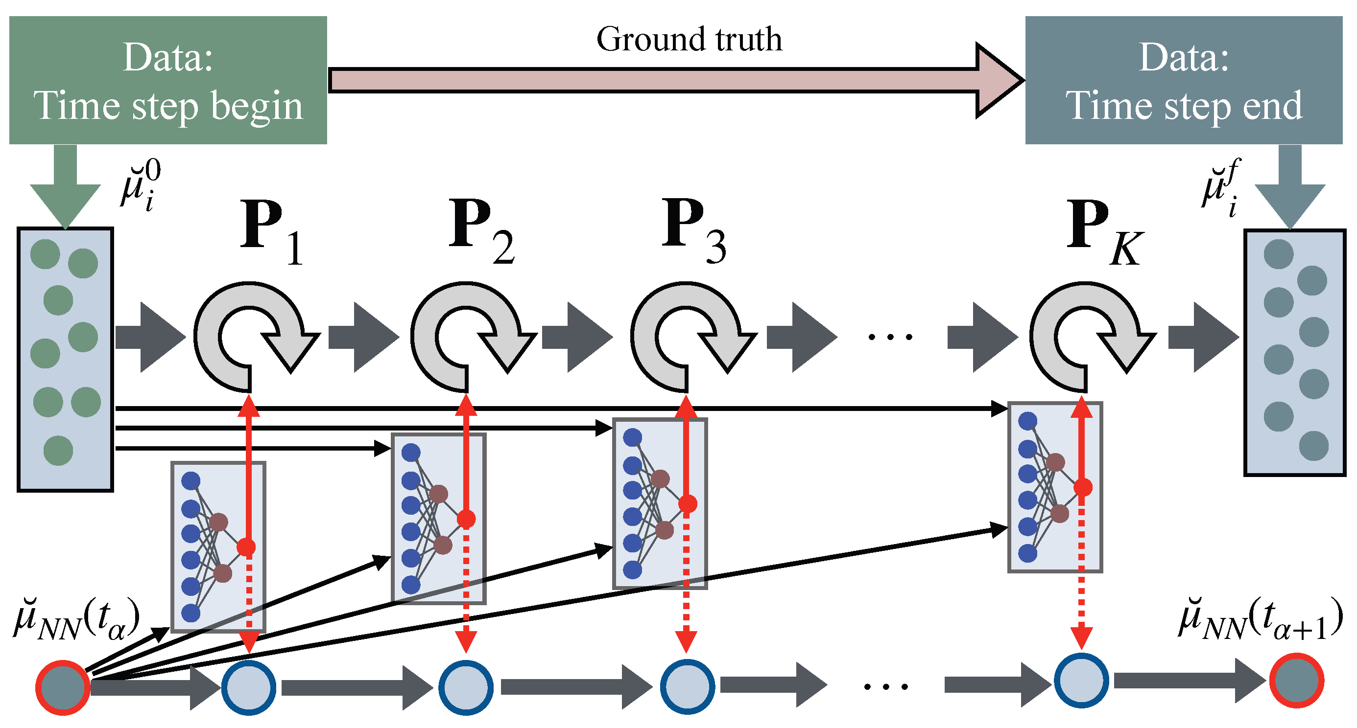
Figure 2.
Trajectory comparison in the case of three particles for group, for the case of ’Democracy’. Ground truth case is denoted with blue colour, while CO-LPNets - with red colour, for one representative trajectory. All components are plotted, with particle index indicated by the row, and the component by the column of the table.
Figure 2.
Trajectory comparison in the case of three particles for group, for the case of ’Democracy’. Ground truth case is denoted with blue colour, while CO-LPNets - with red colour, for one representative trajectory. All components are plotted, with particle index indicated by the row, and the component by the column of the table.
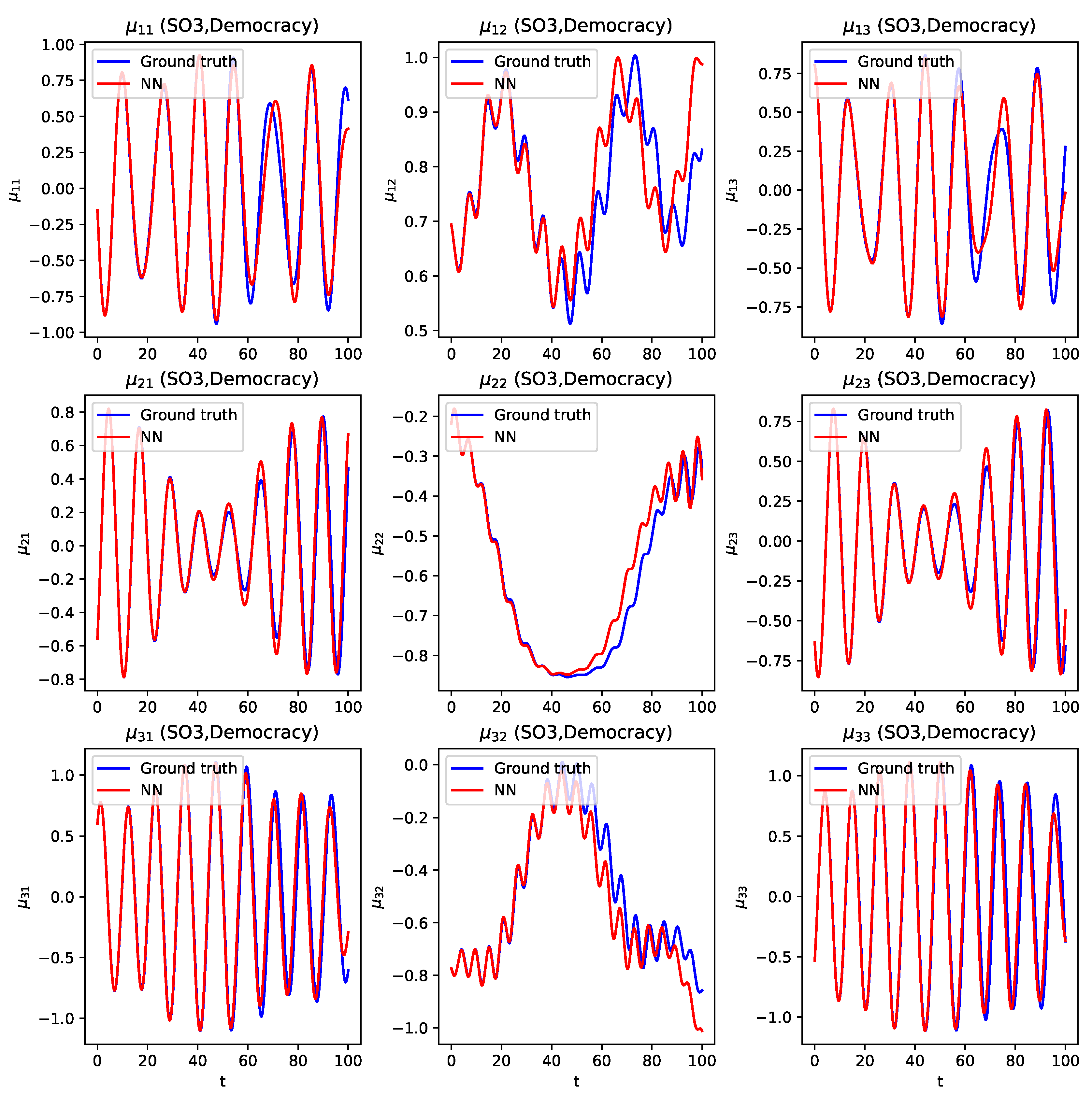
Figure 3.
Errors in the Casimir for each particle (left), Total energy (center) and Mean Absolute Error (MAE, right) for the trajectory presented on Figure 2. MAE is computed for all ten reconstructed solutions, not just for the one shown on Figure 2. Again, ground truth solution is denoted with blue colour, while the results of CO-LPNets are denoted with red colour.
Figure 3.
Errors in the Casimir for each particle (left), Total energy (center) and Mean Absolute Error (MAE, right) for the trajectory presented on Figure 2. MAE is computed for all ten reconstructed solutions, not just for the one shown on Figure 2. Again, ground truth solution is denoted with blue colour, while the results of CO-LPNets are denoted with red colour.
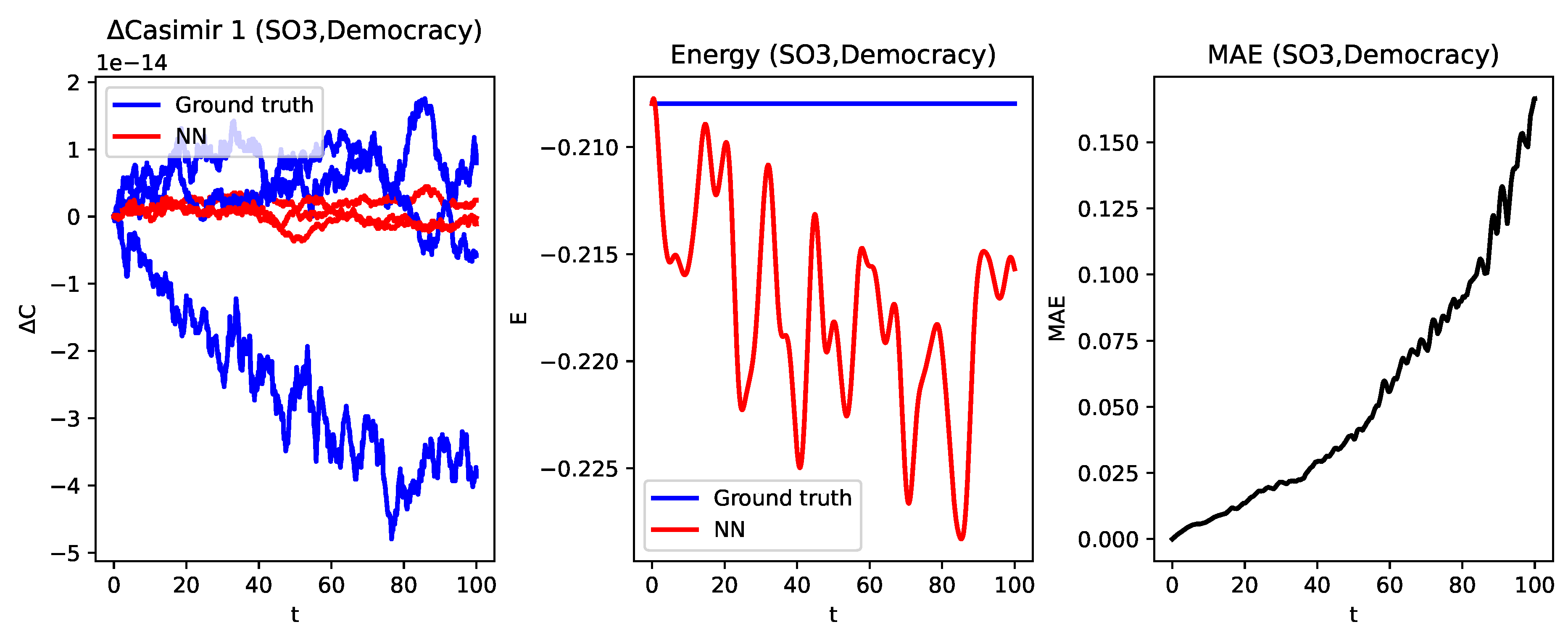
Figure 4.
The comparison of solutions for the case of three particles for group, the ’Dictatorship’ case, with all notations and color scheme as in Figure 2.
Figure 4.
The comparison of solutions for the case of three particles for group, the ’Dictatorship’ case, with all notations and color scheme as in Figure 2.
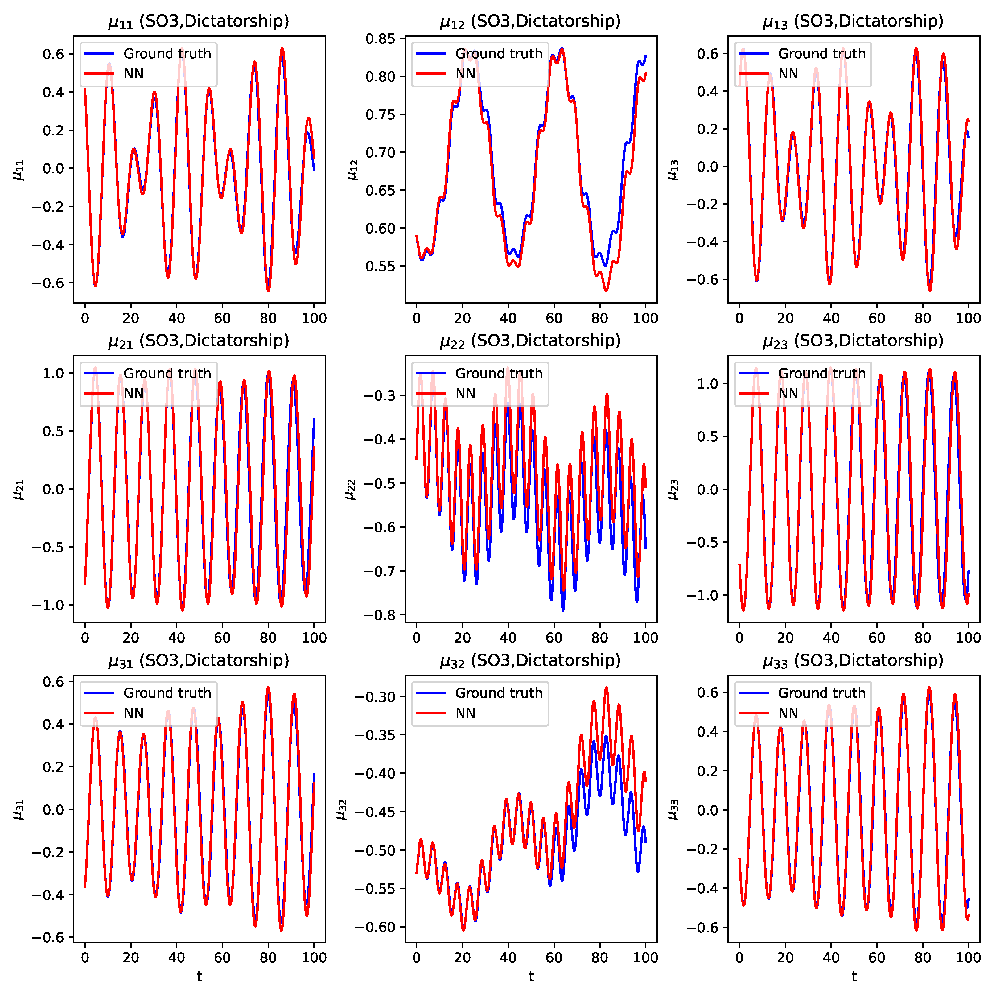
Figure 5.
Errors in the Casimir (left), Energy (center) and Mean Absolute Error (MAE, right) for the sample trajectory presented on Figure 4. Similar to Figure 3, MAE is computed over all sample solutions. Color scheme and notations are the same as in Figure 3.
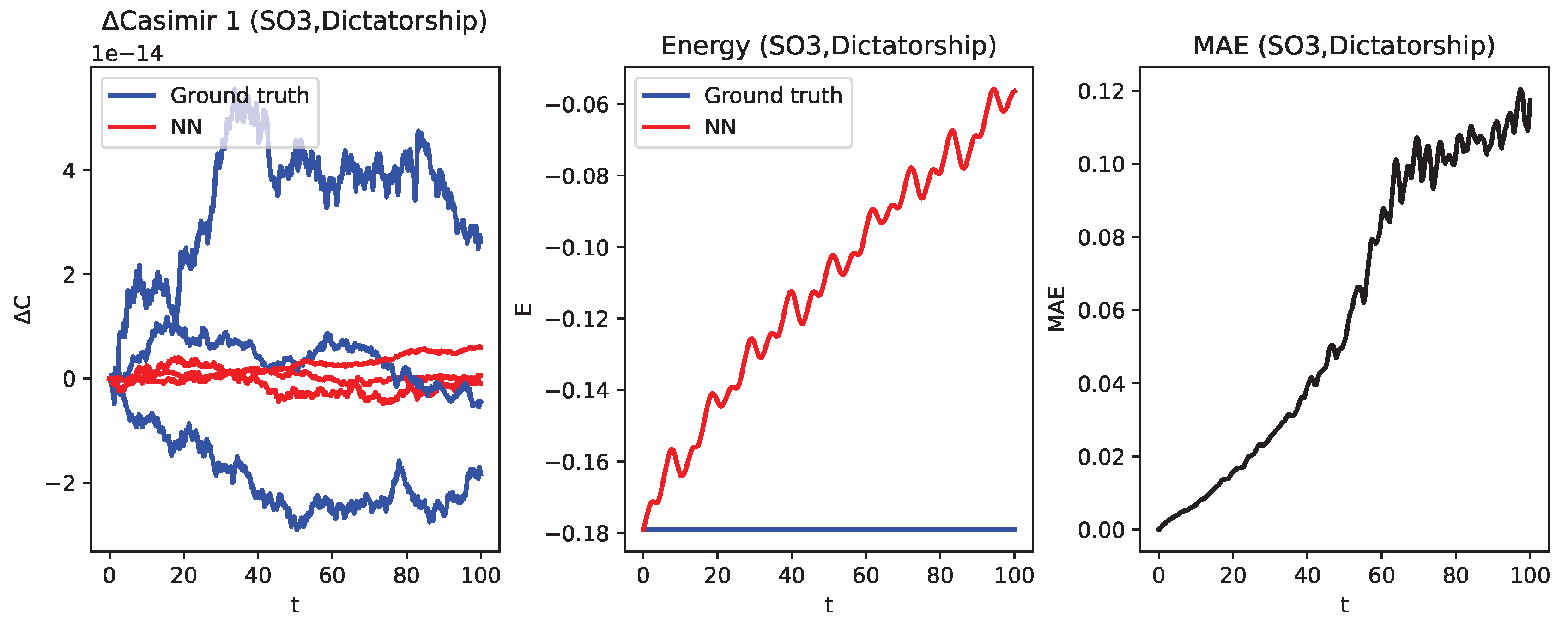
Figure 6.
Trajectory comparison in the case of three particles for group, for the case of ’Democracy’. Ground truth case is denoted with blue colour, while CO-LPNets - with red colour, for one representative trajectory. Only the first three components , are plotted, with particle index indicated by the row, and the component by the column of the table.
Figure 6.
Trajectory comparison in the case of three particles for group, for the case of ’Democracy’. Ground truth case is denoted with blue colour, while CO-LPNets - with red colour, for one representative trajectory. Only the first three components , are plotted, with particle index indicated by the row, and the component by the column of the table.
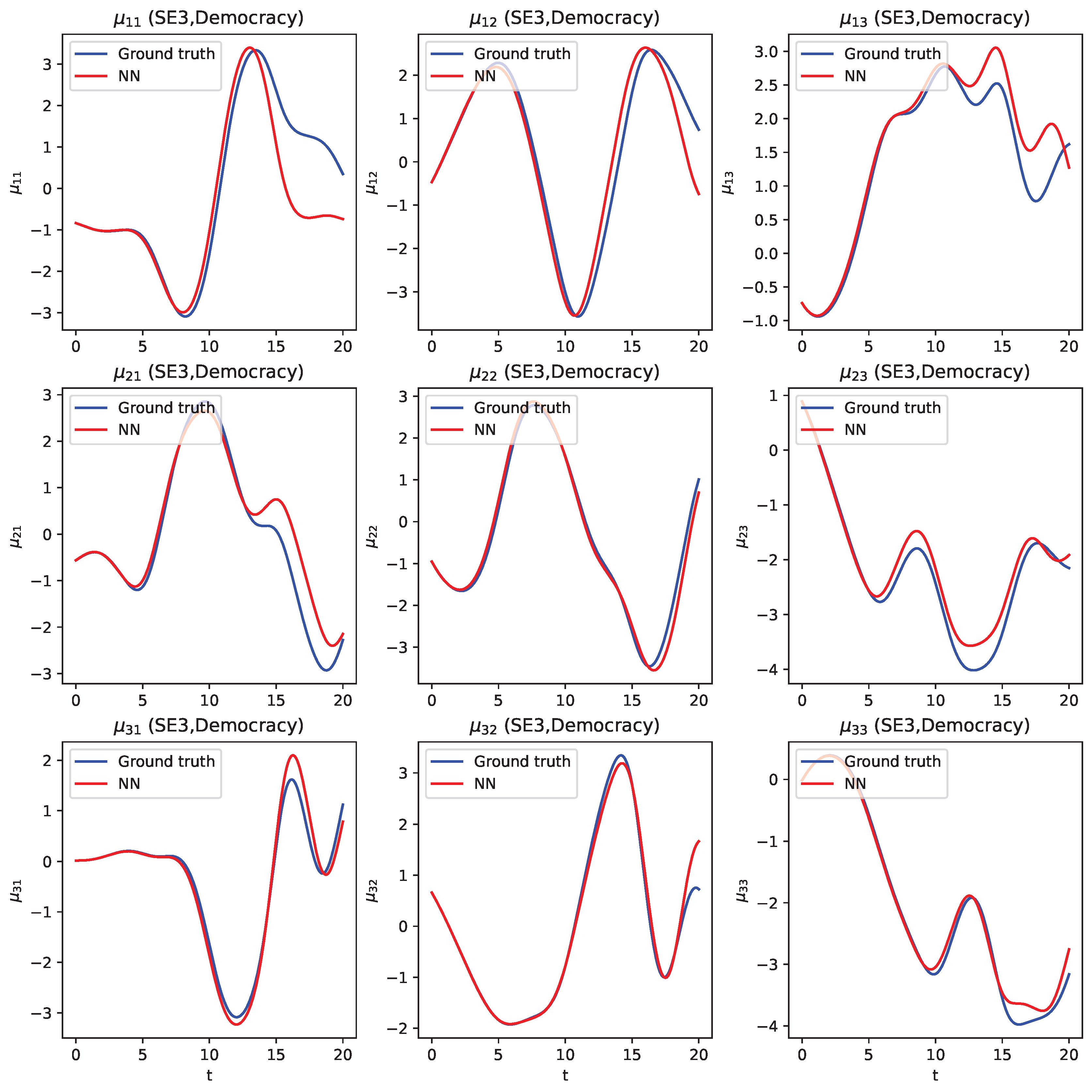
Figure 7.
Conservation of the Casimirs (top), Errors in the energy (bottom left) for a sample trajectory, Mean Absolute Error (MAE) for all ten test trajectories (bottom right), for the case of ’Democracy’ for . Ground truth case is denoted with blue colour, while CO-LPNets are denoted with red colour. Notice, again, preservation of the Casimirs with machine precision, and quite accurate conservation of the energy on average by CO-LPNets.
Figure 7.
Conservation of the Casimirs (top), Errors in the energy (bottom left) for a sample trajectory, Mean Absolute Error (MAE) for all ten test trajectories (bottom right), for the case of ’Democracy’ for . Ground truth case is denoted with blue colour, while CO-LPNets are denoted with red colour. Notice, again, preservation of the Casimirs with machine precision, and quite accurate conservation of the energy on average by CO-LPNets.
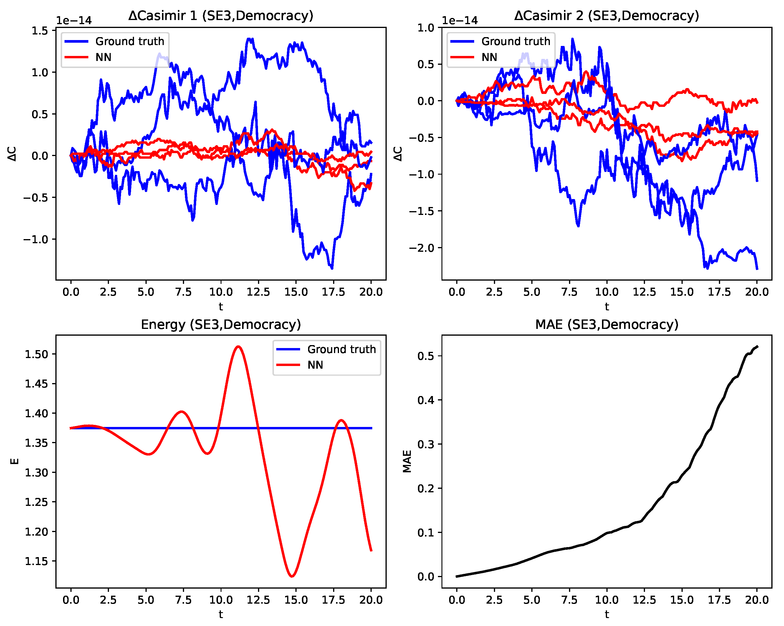
Figure 8.
Trajectory comparison in the case of three particles for group, for the case of dictatorship. Only first three components of six are plotted for every particle, with the number of the particle corresponding to the row in the table, and the component to the column of the table. Color scheme and notations are identical to Figure 6.
Figure 8.
Trajectory comparison in the case of three particles for group, for the case of dictatorship. Only first three components of six are plotted for every particle, with the number of the particle corresponding to the row in the table, and the component to the column of the table. Color scheme and notations are identical to Figure 6.
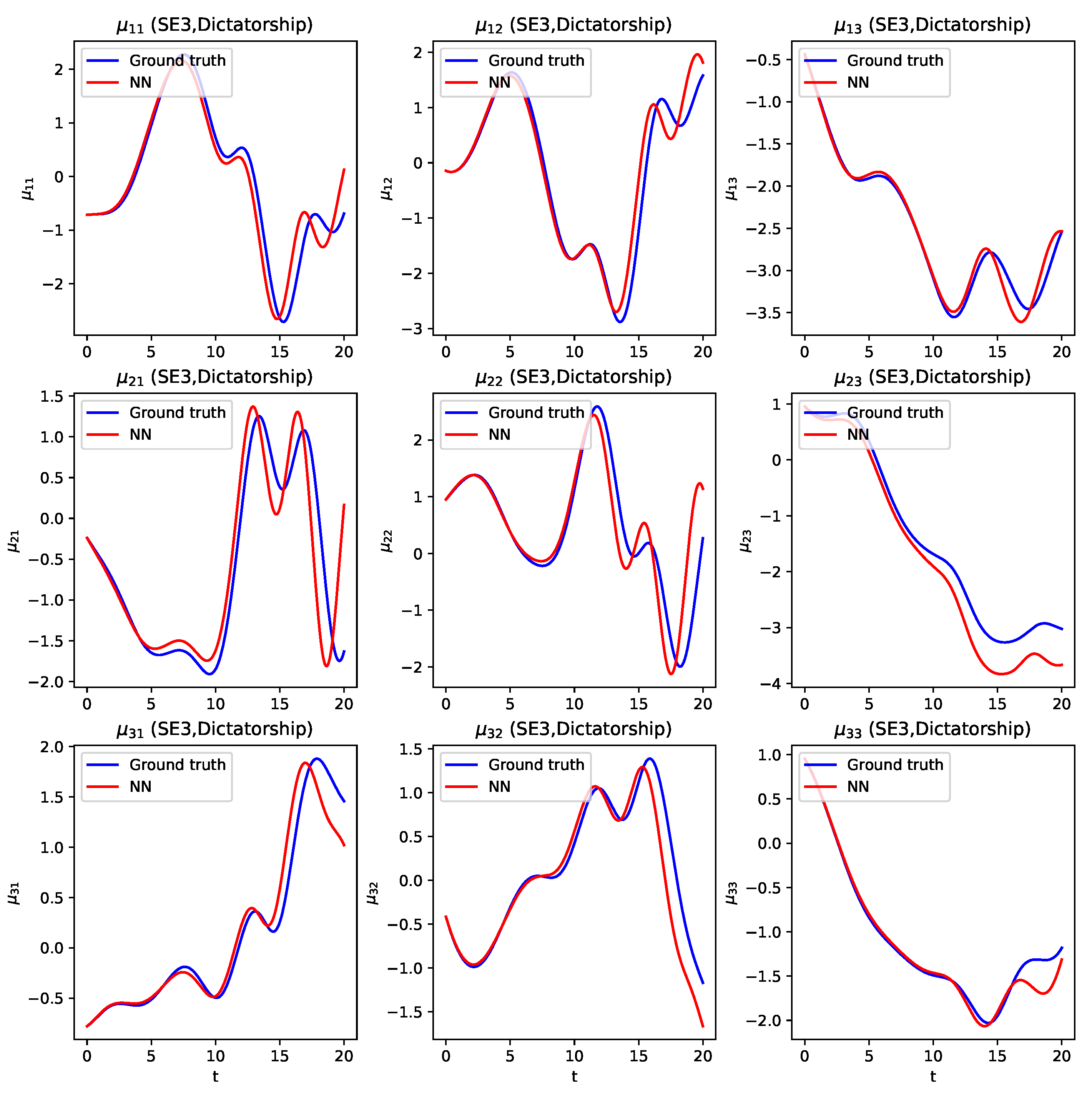
Figure 9.
Summary of ’Dictatorship’ governance for three particles evolving on . Error in Casimirs (top), Errors in the energy (bottom left) and Mean Absolute Error (MAE) for all ten test trajectories (bottom right). Both Casimirs are conserved with machine precision for all particles, as expected. Color scheme and notations are identical to Figure 7.
Figure 9.
Summary of ’Dictatorship’ governance for three particles evolving on . Error in Casimirs (top), Errors in the energy (bottom left) and Mean Absolute Error (MAE) for all ten test trajectories (bottom right). Both Casimirs are conserved with machine precision for all particles, as expected. Color scheme and notations are identical to Figure 7.
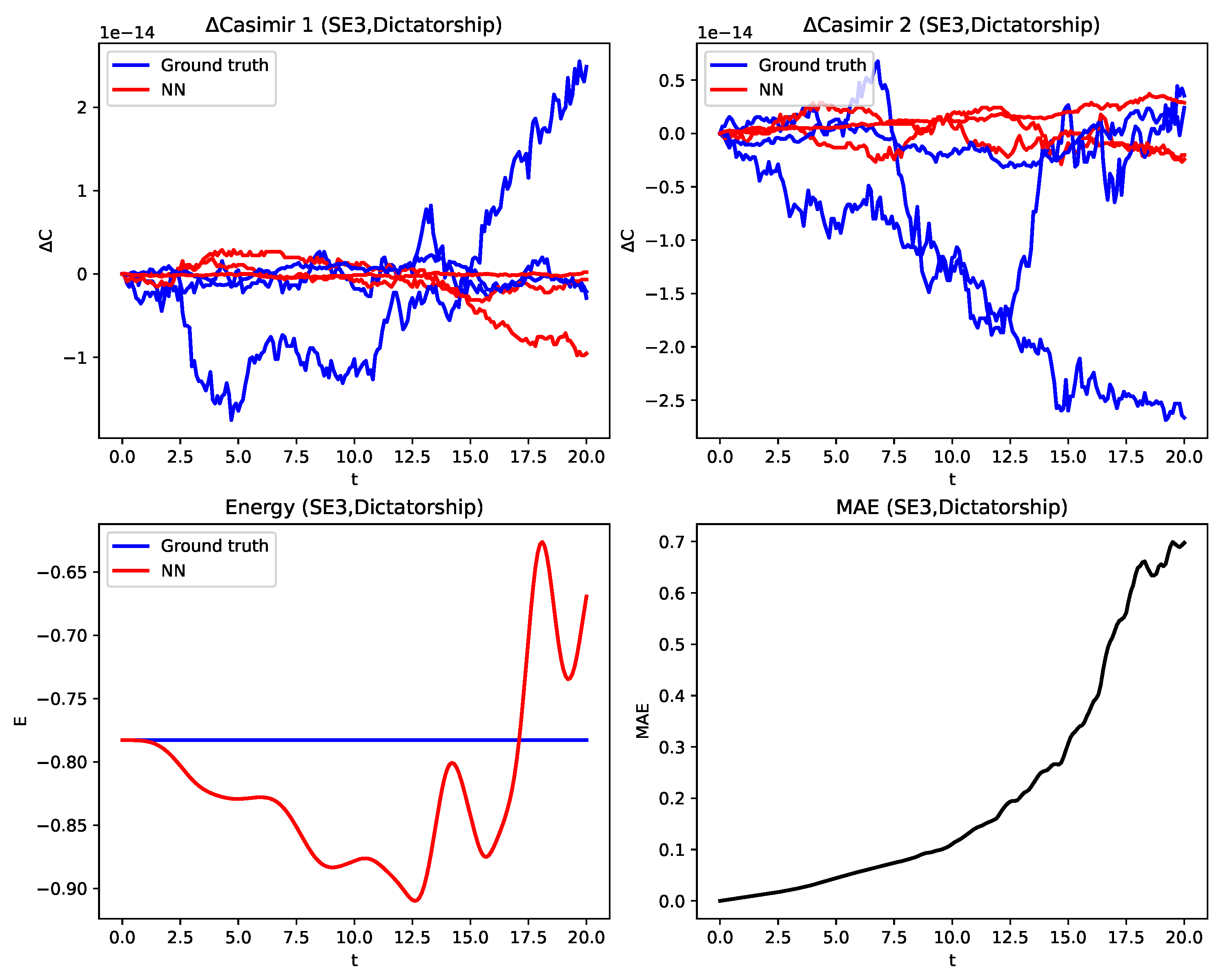
Figure 10.
Trajectory reconstruction performed by the system trained on data corrupted by Gaussian noise , with standard deviations . Color code: Black represents the Ground Truth; Purple represents (clean data); while the blue, cyan, yellow, orange, and red solid lines correspond to and , respectively.
Figure 10.
Trajectory reconstruction performed by the system trained on data corrupted by Gaussian noise , with standard deviations . Color code: Black represents the Ground Truth; Purple represents (clean data); while the blue, cyan, yellow, orange, and red solid lines correspond to and , respectively.
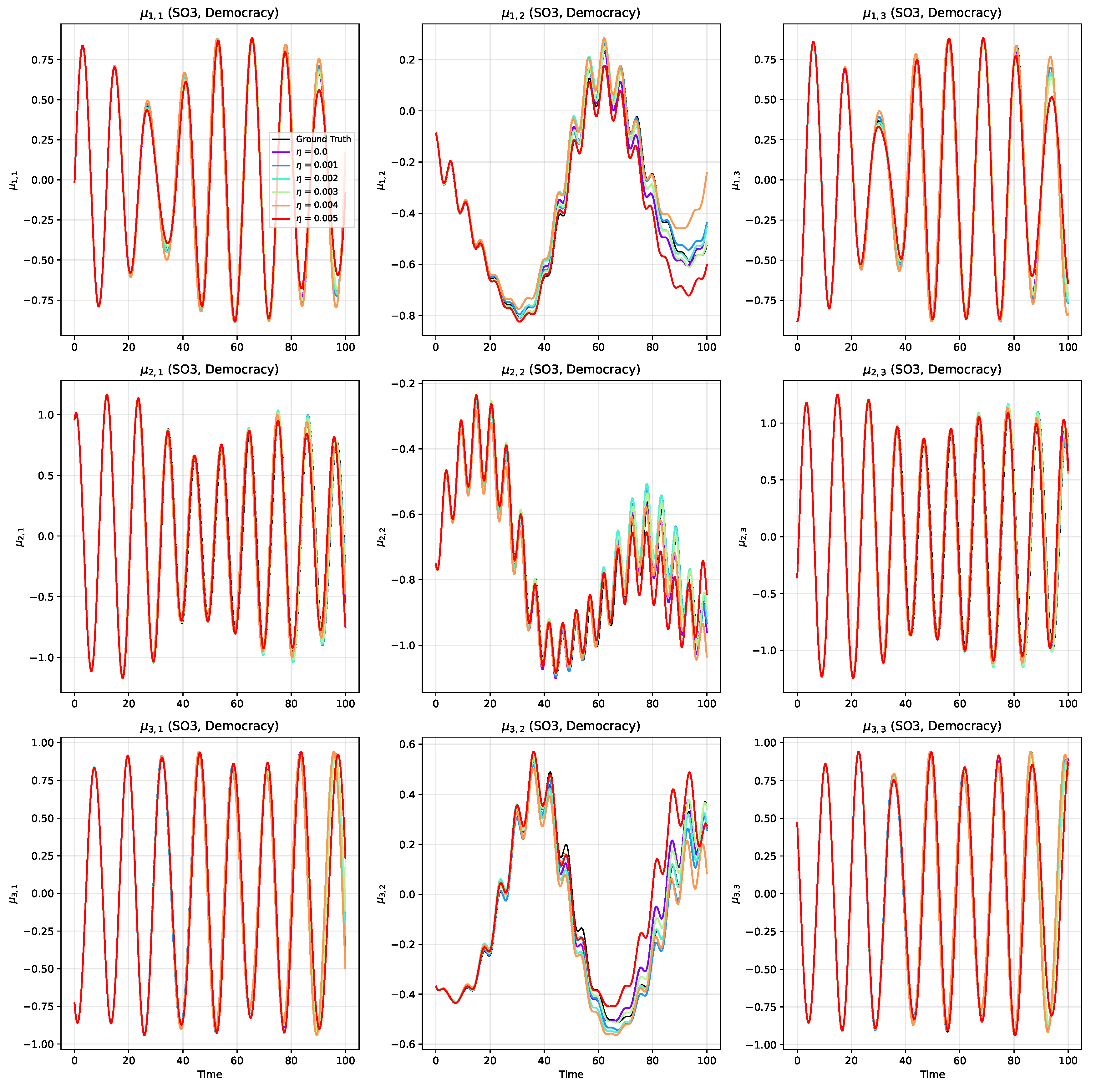
Figure 11.
Quantitative error analysis of the system trained on noisy data. Left: The absolute drift in the Casimir invariants, , confirming preservation to machine precision for all noise levels. Center: The absolute drift in energy conservation, , averaged over all realizations. Right: The Mean Absolute Error (MAE) of the predicted trajectories relative to the ground truth, averaged across all test trajectories, components, and noise realizations. The color code matches that of Figure 10.
Figure 11.
Quantitative error analysis of the system trained on noisy data. Left: The absolute drift in the Casimir invariants, , confirming preservation to machine precision for all noise levels. Center: The absolute drift in energy conservation, , averaged over all realizations. Right: The Mean Absolute Error (MAE) of the predicted trajectories relative to the ground truth, averaged across all test trajectories, components, and noise realizations. The color code matches that of Figure 10.
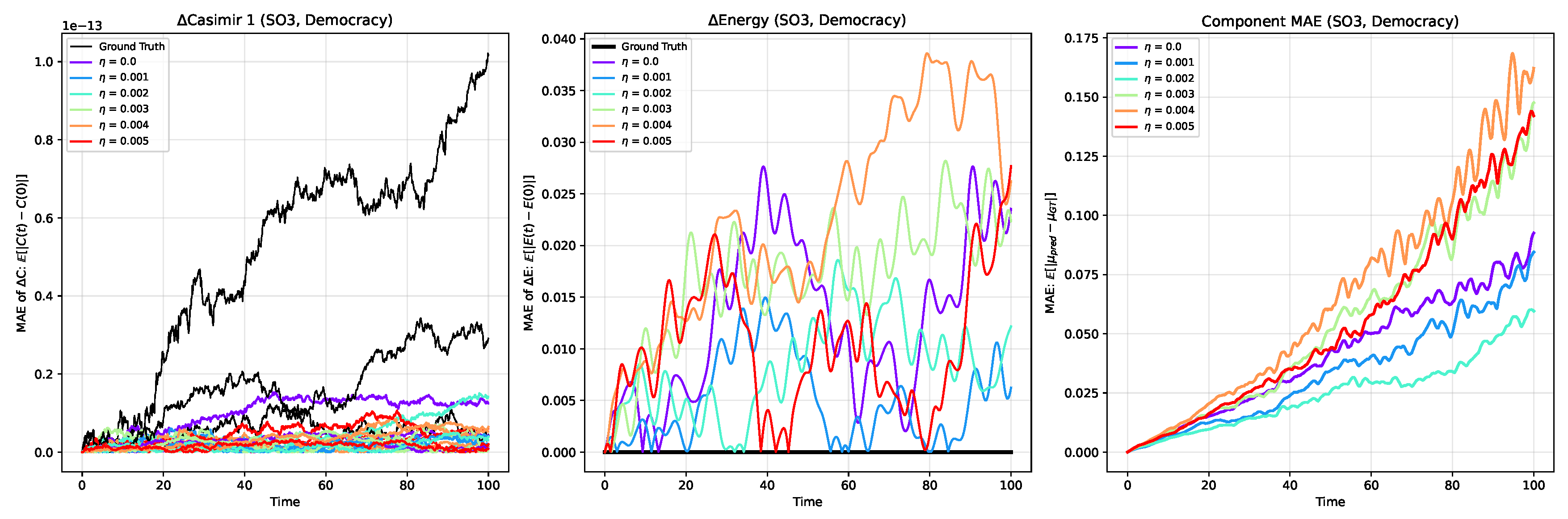
Disclaimer/Publisher’s Note: The statements, opinions and data contained in all publications are solely those of the individual author(s) and contributor(s) and not of MDPI and/or the editor(s). MDPI and/or the editor(s) disclaim responsibility for any injury to people or property resulting from any ideas, methods, instructions or products referred to in the content. |
© 2026 by the authors. Licensee MDPI, Basel, Switzerland. This article is an open access article distributed under the terms and conditions of the Creative Commons Attribution (CC BY) license (http://creativecommons.org/licenses/by/4.0/).
Copyright: This open access article is published under a Creative Commons CC BY 4.0 license, which permit the free download, distribution, and reuse, provided that the author and preprint are cited in any reuse.


