
Submitted:
22 July 2026
Posted:
22 July 2026
You are already at the latest version
Abstract
Wind shear coefficients (WSCs) are fundamental parameters for wind resource assessment, wind turbine design, and offshore wind farm operation. However, the characteristics of WSCs in the offshore waters of Zhuanghe have not yet been systematically investigated. In this study, two years of in-situ observational data (2015-2017) were analyzed to characterize the temporal variability of WSCs under different atmospheric stability conditions. The results indicate that the atmospheric boundary layer in the study area is dominated by stable and unstable conditions, exhibiting a distinct U-shaped annual distribution. The diurnal evolution of atmospheric stability varies considerably among months and is strongly associated with both wind speed and wind direction. Under low wind speed conditions, stable and unstable atmospheres occur with comparable frequencies. As wind speed increases, the occurrence of neutral conditions increases steadily, and the atmosphere becomes predominantly neutral when wind speed exceeds 18.5 m s-1. Northerly winds are generally associated with unstable atmospheric conditions, whereas southerly winds are primarily associated with stable conditions. The WSC ranges from 0.01 to 0.32 and exhibits pronounced seasonal and monthly variability. Under neutral and unstable atmospheric conditions, the diurnal variation of WSC is relatively consistent across different measurement heights. In contrast, under stable conditions, significant vertical differences in WSC are observed throughout most of the year, except in March and April. These findings improve the understanding of offshore wind shear characteristics under different atmospheric stability regimes and provide valuable guidance for offshore wind resource assessment, wind profile modeling, and the design, operation, and optimization of offshore wind farms in the Zhuanghe offshore region.
Keywords:
meteorological data
; wind shear coefficient
; atmospheric stability
; Zhuanghe offshore
; power law model
1. Introduction
To meet the growing global demand for energy and mitigate ongoing climate change and environmental degradation, the development and utilization of renewable energy sources are essential for advancing the global energy transition [1]. As one of the major renewable energy sources, wind energy has experienced rapid growth worldwide, driven by supportive national policies and technological progress [2].
China’s offshore wind energy industry has developed rapidly over recent decades [3]. By the end of 2025, China is expected to have further consolidated its position as a leading force in the global offshore wind sector. WSC is a key parameter for resource assessment, offshore wind farm construction, and operational management [4]. Its variation is affected by multiple meteorological and environmental factors, including atmospheric conditions, air temperature, atmospheric pressure, humidity, wind speed, wind direction, and terrain type [5]. In addition, WSC exhibits diurnal, weekly, and seasonal variability, among other temporal patterns [6,7].
Over the past two decades, extensive research has been conducted on WSCs from various perspectives, including its temporal variability, influencing factors, and applications in wind energy assessment. Smith et al. (2002) investigated the diurnal variation of WSC and its relationship with wind turbine faults [8]. Frandsen (2005) examined the influence of WSC on atmospheric turbulence and turbulence-induced fatigue loading of wind turbines [9]. Du et al. (2010) analyzed the monthly and diurnal variations of WSC and demonstrated its application in wind resource assessment [10]. Li et al. (2012) characterized the diurnal variation of WSC using observations from the China Wind Energy Resource Professional Observation Network [11]. Li et al. and Peng et al. (2010) investigated methods for calculating WSC and evaluated its influence on wind resource assessment [12,13].
Several studies have further revealed the spatial and seasonal characteristics of WSC. Farrugia (2003) reported significant seasonal variations, with WSC reaching a maximum value of 0.45 in January and a minimum of 0.29 in August [14]. Yuan et al. (2024) analyzed daily and monthly variations of WSC using data collected from 754 land wind measurement towers across China and proposed representative WSC values for different land-cover types [15]. Pearre et al. (2025) identified pronounced seasonal variability in vertical wind shear over the northwestern North Atlantic based on long-term anemometer observations [16]. Geonhwa Ryu et al. (2023) demonstrated that offshore WSC is strongly correlated with sea surface temperature [17]. Debnath et al. (2023) also reported significant diurnal and seasonal variability in WSC [18], while Borvaran et al. (2021) observed relatively large vertical wind shear values in Southern New England [19].
The influence of WSC on wind energy production has also been extensively investigated. Murphy (2020) showed that WSC has a significant impact on wind power generation [20]. Rehman (2008) and Firtin (2011) demonstrated that assuming a constant WSC may lead to either underestimation or overestimation of wind energy potential [21,22]. More recently, Wu et al. (2026) analyzed the diurnal and monthly variations of WSC using observational data from a wind farm in Inner Mongolia and developed a hybrid physics-informed and data-driven wind profile model [23].
In China, several regional studies have focused on offshore and coastal wind shear characteristics. Shu (2020) and Yan (2022) investigated the diurnal and seasonal variations of WSC using LiDAR measurements from an offshore observation station in southwestern Hong Kong [24,25]. Chen (2019) analyzed the variation of WSC in the coastal region of Jiangsu Province and further examined its characteristics under strong wind conditions [26].
The offshore area of Zhuanghe, Liaoning Province, is one of the most promising regions for offshore wind energy development in China due to its abundant wind resources [27,28]. Several offshore wind farms have been commissioned in this area, and more projects are currently under construction or in the planning stage [29,30]. At the same time, the continuous increase in hub height and rotor diameter of modern offshore wind turbines has made the accurate characterization of the vertical wind profile increasingly important for reliable wind resource assessment and energy yield prediction [31]. As a key parameter describing the vertical distribution of wind speed, the WSC plays a crucial role in wind farm siting, turbine design, wake modeling, and operational optimization. Nevertheless, the characteristics of offshore WSC over the Zhuanghe sea area remain poorly understood, and the effects of atmospheric stability on its temporal variability have not been comprehensively evaluated. To address these knowledge gaps, this study investigates the diurnal, monthly, and seasonal variations of offshore WSC in the Zhuanghe offshore area based on long-term observational data, with particular emphasis on the influence of atmospheric stability. The results provide a scientific basis for offshore wind resource assessment and the design and operation of future offshore wind farms in this region.
The remainder of this paper is organized as follows. Section 2 describes the study area, observational site, and meteorological measurements. Section 3 introduces the data quality control procedures, the method used to calculate the WSC, and the atmospheric stability classification method. Section 4 presents the temporal characteristics of WSC under different atmospheric stability conditions and discusses the corresponding results. Finally, Section 5 summarizes the main conclusions and their implications for offshore wind resource assessment and wind farm development.
2. Study Area and Data Description
Figure 1 presents the location of the study area (38.5°–41.0°N, 122.0°–124.5°E) in the northern Yellow Sea, adjacent to Zhuanghe City on the Liaodong Peninsula. The region is characterized by a typical East Asian monsoon climate [32]. The winter monsoon prevails from October to March and is dominated by northerly, particularly northwesterly, winds, whereas the summer monsoon extends from May to August with prevailing southerly and southwesterly winds. April and September are transitional months between the two monsoon systems. During April, the winter monsoon gradually weakens and is replaced by the summer monsoon, while in September the summer monsoon retreats rapidly and the winter monsoon becomes re-established [33].
The field measurements were conducted at an offshore wind farm located in the northern Yellow Sea, approximately 12 km off the coast of Zhuanghe, Liaoning Province. As illustrated in Figure 1, the location of Zhuanghe City is marked by a solid black dot, and the meteorological mast is indicated by a yellow triangle. The mast was instrumented with multiple sensors mounted on horizontal booms at heights ranging from 20 to 100 m above mean sea level (MSL). These instruments continuously measured wind speed, wind direction, and air temperature. Detailed specifications of the measurement systems are provided in Table 1.
To enhance measurement reliability, two independent wind measurement systems, NRG (USA) and Risø (Denmark), were installed at each observation level. Continuous meteorological observations were collected from 13 November 2015 to 12 November 2017, providing a two-year dataset for subsequent analysis.
3. Methods
3.1. Data Quality Control
Quality control procedures were applied to the 10 min averaged observations collected from the meteorological mast before further analysis. The dataset was screened according to the following criteria.
(1) Range check. The valid ranges of the measured meteorological variables were defined as 0.5–30.0 m s⁻¹ for wind speed, 0°–360° for wind direction, and −35 to 35 °C for air temperature [36].
(2) Vertical temperature consistency check. The air temperature difference between between consecutive measurement heights was required to be less than 2 °C.
(3) Wind direction consistency check. For the two independent wind direction measurements at the same height, the difference was required to be within ±15° [37].
(4) Wind speed consistency check. As shown in Figure 3, the relative difference between the wind speeds measured by the NRG and Risø systems at the same height was required to be less than 30%.
(5) Wind profile consistency check. Only wind speed profiles showing a monotonic increase with height were retained for subsequent analysis.
For each observation level, the final wind speed was calculated as the average of the two valid measurements obtained from the NRG and Risø systems. If either instrument failed to satisfy the quality control criteria at a given height, the corresponding observations from both instruments at that height were discarded [38].
After applying the above quality control procedures, a high-quality datasets was obtained for subsequent statistical analysis.
Following quality control, approximately 97.07% of the original observations were retained for subsequent analysis.
3.2. Wind Shear Coefficient (WSC)
The wind shear coefficient (WSC) is a dimensionless parameter that characterizes the variation of wind speed with height. In wind resource assessment and wind energy applications, wind speeds measured at a reference height are commonly extrapolated to target elevations, such as wind turbine hub heights, using either the power-law or logarithmic wind profile model. In this study, the power-law model was adopted because of its computational efficiency and widespread use in engineering applications [39,40,41,42,43,44]. The model, originally proposed by Hellmann in 1914 [45], is expressed as follows:
where and denote the wind speeds measured at heights and , respectively, and is the Hellmann exponent, also referred to as the wind shear coefficient (WSC). The WSC can be determined from wind speed measurements at two different heights. Based on Equation (1), the WSC can be derived by taking the natural logarithm of both sides and rearranging the equation, yielding:
3.3. Atmospheric Stability Classes
Atmospheric stability was classified using the bulk Richardson number (), a dimensionless parameter that quantifies the balance between buoyancy and mechanical turbulence. Owing to its computational efficiency and extensive use in studies of the atmospheric boundary layer, () has been widely adopted as a practical indicator of atmospheric stability. In this study, () was calculated from concurrent measurements of air temperature and wind speed at multiple observation heights. It is expressed as follows [46]:
For open-sea conditions, Equation (3) can be simplified as follows [47]:
where is the air temperature, is the sea surface temperature (SST), is the wind speed measured at height , is the measurement height above sea level, and is the gravitational acceleration. The SST data used in this study were obtained from the Operational Sea Surface Temperature and Sea Ice Analysis (OSTIA) product [48]. Based on the calculated bulk Richardson number [46,47], atmospheric stability was classified into stable, neutral, and unstable conditions according to Table 2.
4. Results and Analysis
4.1. Monthly Variation of the Atmospheric Stability
Figure 2 presents the monthly distributions of atmospheric stability at four measurement heights (20, 50, 80, and 100 m), together with the monthly variation in the air–sea temperature difference. The annual occurrence frequencies of the three atmospheric stability regimes are summarized in Table 3. The proportions of stable, neutral, and unstable conditions exhibit only minor variations with height, indicating that atmospheric stability over the study area is largely independent of the measurement elevation.
A pronounced seasonal cycle is observed in atmospheric stability. Stable conditions exhibit a distinct U-shaped annual distribution, with the lowest occurrence frequencies during winter and the highest during late spring and summer. Conversely, unstable conditions display an approximately symmetric seasonal pattern, dominating during January, February, November, and December. From March onward, the frequency of stable conditions increases steadily, while that of unstable conditions decreases. Stable conditions become dominant from May to July. Beginning in August, the occurrence of neutral and unstable conditions gradually increases, and unstable conditions again become dominant during late autumn and early winter.
The seasonal variation in atmospheric stability is closely associated with the air–sea temperature difference. As shown in Figure 2, large negative air–sea temperature differences occur during January, February, October, November, and December, corresponding to predominantly unstable atmospheric conditions. In March, August, and September, the air–sea temperature difference is close to zero, resulting in the coexistence of stable, neutral, and unstable conditions. During April–July, the air temperature is generally higher than the sea surface temperature, leading to positive air–sea temperature differences and a predominance of stable atmospheric conditions.
This behavior can be attributed to seasonal changes in the thermal contrast between the sea surface and the overlying atmosphere. During winter, the relatively warm sea surface heats the lower atmosphere, promoting buoyancy-driven turbulence and unstable stratification. In contrast, during late spring and summer, the warmer air over the cooler sea suppresses vertical turbulent mixing, resulting in predominantly stable atmospheric conditions.
4.2. Diurnal Variation of the Atmospheric Stability
Figure 3 presents the diurnal variations in atmospheric stability during the four transitional months (March, April, August, and September) at a height of 20 m. These four months are the only periods during which stable, neutral, and unstable atmospheric conditions coexist (Figure 2).
Distinct diurnal variations in atmospheric stability are observed in March and September, whereas such variations are much weaker in April and August. In March, unstable conditions dominate throughout the day but exhibit pronounced diurnal variability, with the highest occurrence frequency at approximately 05:00 and the lowest at around 16:00. Compared with March, the atmospheric stability regime changes markedly in April, when stable conditions become dominant and the diurnal variation is substantially reduced. August exhibits a similar stability pattern to April, although slight diurnal fluctuations are still evident.
Among the four transitional months, September exhibits the most pronounced diurnal cycle. A clear day–night reversal in atmospheric stability is observed, with unstable conditions occurring predominantly during the daytime and stable conditions prevailing at night. This behavior reflects the strong influence of the diurnal heating and cooling cycle during the seasonal transition from summer to winter.
The weak diurnal variation observed in April and August suggests that seasonal-scale thermal forcing dominates over the diurnal heating cycle during these months.
The pronounced diurnal cycle in September is likely associated with enhanced land–sea thermal contrast during the transition from the summer to the winter monsoon.
4.3. Atmospheric Stability Versus Wind Speed
Figure 4 presents the occurrence frequencies of stable, neutral, and unstable atmospheric conditions as a function of wind speed at the 20 m observation level. Wind speeds recorded during the two-year observation period ranged from 0.5 to 21.9 m s⁻¹ and were classified into 2.0 m s⁻¹ bins.
A clear relationship is observed between atmospheric stability and wind speed. At low wind speeds (<4.5 m s⁻¹), stable conditions occur most frequently. As wind speed increases, the occurrence of stable conditions decreases continuously, whereas the frequency of neutral conditions increases. The occurrence of unstable conditions changes only slightly at low and moderate wind speeds but decreases rapidly at higher wind speeds. Above 18.5 m s⁻¹, unstable conditions are no longer observed, and the atmosphere is almost entirely neutral. At the highest wind speed range, all observations are classified as neutral conditions.
The predominance of neutral conditions under high wind speeds is consistent with previous studies, indicating that mechanically generated turbulence becomes increasingly dominant over buoyancy effects as wind speed increases.
4.4. Atmospheric Stability Versus Wind Direction
As shown in Figure 5, the distribution of atmospheric stability varies considerably with wind direction during different monsoon periods. Wind direction was classified into 16 sectors with an interval of 22.5°. According to the seasonal evolution of the East Asian monsoon, the observations were divided into four representative periods: (1) the winter monsoon period (January, February, October, November, and December; Figure 5a), (2) the transition from winter to summer (March and April; Figure 5b), (3) the summer monsoon period (May–July; Figure 5c), and (4) the transition from summer to winter (August and September; Figure 5d).
Figure 5 illustrates the distribution of atmospheric stability classes under different wind directions for four periods. In panel (a), the distribution is strongly dominated by northerly winds, and unstable conditions account for the vast majority of occurrences. This indicates that, during this period, atmospheric conditions are primarily characterized by unstable stratification associated with a concentrated northern wind sector. In panel (b), the wind direction distribution becomes more dispersed, while stable and neutral conditions increase substantially, suggesting a transitional state from an unstable-dominated regime to a more mixed atmospheric structure. In panel (c), stable conditions become overwhelmingly dominant, with the highest frequencies occurring in the southeasterly to southerly sectors. This suggests a strong association between stable stratification and winds from the SE–S sector during this period. In panel (d), stable conditions remain dominant, although neutral and unstable classes reappear in several wind sectors, resulting in a more complex but still stability-dominated distribution. Overall, the figure demonstrates a clear relationship between wind direction and atmospheric stability, with both the prevailing wind sector and the dominant stability regime varying markedly across the four periods.
Overall, atmospheric stability exhibits a pronounced dependence on wind direction that is closely linked to the seasonal evolution of the East Asian monsoon. Northerly winds are generally associated with unstable atmospheric conditions, whereas southerly winds are predominantly accompanied by stable stratification. This relationship reflects the combined influence of monsoon circulation and air–sea thermal contrast on the stability of the marine atmospheric boundary layer.
4.5. Diurnal Variation of Wind Shear Coefficient Under Different Atmospheric Stability
Hourly WSCs were calculated using the power-law model based on wind speeds measured at different observation heights. As listed in Table 4, () denotes the WSC calculated from wind speeds measured at 20 m and 50 m, while () and () are defined in the same manner. This section focuses on the diurnal variations of WSC between 20 m and the higher observation levels (50, 80, and 100 m) under unstable, neutral, and stable atmospheric conditions.
Figure 6 summarizes the diurnal evolution of WSC under different atmospheric stability regimes. Different colors represent different months, while different symbols denote the three height pairs. Overall, WSC exhibits pronounced seasonal variability, and its diurnal characteristics differ considerably among the three atmospheric stability regimes.
Figure 6a presents the diurnal variations of WSCs under unstable atmospheric conditions. For a given month, the WSC curves corresponding to the three height pairs , , and are closely clustered throughout the day, indicating that the vertical distribution of WSC is only weakly dependent on height under unstable conditions. In contrast, pronounced monthly variability is observed. March exhibits the highest WSC values, ranging from approximately 0.15 to 0.25, followed by February with values between 0.10 and 0.16. During the remaining months, WSC generally remains below 0.10, while August records the lowest values, mostly below 0.03. From August onward, WSC gradually increases towards winter, with a more rapid increase occurring after January. Moreover, the diurnal amplitudes during January–March are substantially larger than those observed from August to December, indicating stronger temporal variability during late winter and early spring. The weak dependence of WSC on height under unstable conditions suggests that buoyancy-driven turbulence effectively enhances vertical mixing, resulting in relatively uniform wind shear characteristics throughout the lower marine atmospheric boundary layer.
Figure 6b illustrates the diurnal evolution of WSC under stable atmospheric conditions. Compared with the unstable regime, the WSC exhibits considerably stronger diurnal and vertical variations. For most months, WSC gradually increases from the afternoon towards the evening, reaches its maximum during 20:00–22:00, and then decreases after midnight, with daily minima generally occurring between 07:00 and 10:00. Significant seasonal differences are also evident. March and April exhibit the largest WSC values, with the maximum exceeding 0.32 in March. In contrast, September records the lowest WSC values among all stable months. Unlike the unstable regime, distinct vertical differences are observed under stable conditions. Except for March and April, WSC consistently increases with increasing height interval, following the relationship >>. This result indicates that stable atmospheric stratification suppresses turbulent mixing and enhances the vertical wind speed gradient, leading to increasingly larger wind shear over greater height intervals. The relatively small differences among the three height pairs in March and April imply that the atmospheric boundary layer remains well mixed during the seasonal transition despite the occurrence of stable conditions.
Figure 6c shows the diurnal characteristics of WSC under neutral atmospheric conditions. Neutral conditions occur only during March, August, and September. Similar to the unstable regime, the WSC curves corresponding to the three height pairs remain closely grouped within each month, indicating weak vertical dependence of WSC under neutral atmospheric conditions. Distinct seasonal differences are nevertheless observed. March exhibits the highest WSC values (approximately 0.15–0.23), followed by August (0.08–0.13), whereas September records the lowest values (0.03–0.06). The magnitude of the diurnal variation also decreases progressively from March to September, with March showing the strongest diurnal fluctuations and September exhibiting relatively stable WSC throughout the day. The similarity among different height pairs suggests that mechanical turbulence dominates the vertical transport under neutral conditions, resulting in a relatively uniform wind profile despite noticeable seasonal changes in WSC magnitude.
The results indicate that atmospheric stability exerts a stronger influence on WSC than seasonal variability alone. Under unstable and neutral conditions, efficient turbulent mixing weakens the vertical wind speed gradient, resulting in similar WSC values among different height pairs. In contrast, stable stratification suppresses vertical turbulent exchange, leading to pronounced height-dependent WSCs and stronger diurnal variability. These findings suggest that the use of a constant wind shear coefficient may introduce substantial uncertainty in offshore wind resource assessment, particularly under stable atmospheric conditions, where WSC exhibits both strong temporal variability and significant vertical dependence.
5. Conclusions
This study investigated the characteristics of atmospheric stability and wind shear coefficient (WSC) over the northern Yellow Sea using two years of meteorological mast observations collected from November 2015 to November 2017. The temporal variability of atmospheric stability and its relationships with wind speed, wind direction, and WSC were systematically analyzed. The main conclusions are summarized as follows.
(1) The atmospheric boundary layer over the study area is dominated by stable and unstable conditions, exhibiting a distinct U-shaped seasonal distribution. Stable conditions prevail from May to July, whereas unstable conditions dominate during January, February, November, and December. Transitional months are characterized by the coexistence of stable, neutral, and unstable conditions. The seasonal evolution of atmospheric stability is closely associated with the East Asian monsoon and is strongly correlated with the air–sea temperature difference.
(2) Pronounced diurnal variations in atmospheric stability are observed during the transitional months of March and September. March is characterized predominantly by unstable conditions, whereas stable conditions prevail in September. In contrast, only weak diurnal variations are observed in April and August, during which stable stratification remains dominant.
(3) Atmospheric stability exhibits strong dependence on both wind speed and wind direction. Under low wind speed conditions (0.5–4.5 m s⁻¹), stable and unstable conditions occur with comparable frequencies. As wind speed increases, neutral conditions become increasingly dominant, and the atmosphere becomes almost entirely neutral when wind speed exceeds 18.5 m s⁻¹. Atmospheric stability also varies systematically with wind direction, reflecting the influence of the East Asian monsoon. Northerly winds are generally associated with unstable conditions, whereas southerly winds are predominantly associated with stable conditions.
(4) The WSC in the study area ranges from 0.01 to 0.32 and exhibits pronounced monthly and diurnal variability. Under neutral and unstable atmospheric conditions, WSCs calculated from different height pairs are highly consistent, indicating weak vertical dependence. In contrast, under stable conditions, significant vertical differences are observed for most months, with the exception of March and April.
Overall, this study provides a comprehensive characterization of atmospheric stability and offshore WSC over the northern Yellow Sea. The results improve the understanding of marine atmospheric boundary-layer characteristics and provide useful guidance for offshore wind resource assessment, wind profile modeling, turbine design, and the planning, operation, and optimization of offshore wind farms in the study region.
Author Contributions
L.C. and H.Z. led the manuscript writing, data processing and result analysis. L.C. and Y.Z. drafted the paper, and Z.Y. and L.H. led the quality control of the datasets. Y.F. and W.Z. conducted the programming and data visualization. W.A. reviewed and edited the manuscript. All authors have read and agreed to the published version of the manuscript.
Funding
This research was funded by Satellite Remote Sensing Information Services (Grant No.2025-JW34-F5001) and Integration and Application Demonstration in the Marine Field (Grant No.0404130306).
Data Availability Statement
The field observation data generated in this study are not publicly available due to data sharing restrictions of the research project. Researchers who require the datasets for replication may contact the corresponding author with a reasonable request.
Acknowledgments
We acknowledge the Operational Sea Surface Temperature and Sea Ice Analysis (OSTIA) product for providing sea surface temperature (SST) data used in this study.
Conflicts of Interest
The authors declare no conflicts of interest.
References
- Xu, S.; Yin, G.; Hu, P. Substantially Lower Estimates in China’s Offshore Wind Potential Using Farm-Scale Spatial Modeling and Wake Effects. Nat. Commun. 2026, 17, 1–15. [Google Scholar] [CrossRef]
- Summerfield-Ryan, O. The Power of Wind: The Global Wind Energy Industry’s Successes and Failures. Ecol. Econ. 2023, 210, 107841. [Google Scholar] [CrossRef]
- Ji, Y.S.; Cheng, J.; Ma, S.D.; Yao, F.R.; Ao, L.Z.; Zhang, J. Reliability Validation of Floating Lidar Measurements and Wind Resource Characteristics within 300 m Height in the South China Sea. J. Mar. Meteorol. 2026, 46. [Google Scholar]
- Hua, Z.; Tao, W.; Wang, G. Wind Resource Evaluation With Atmospheric Stability Across Different Surface Types. Energy Sci. Eng. 2026, 14. [Google Scholar] [CrossRef]
- Firtin, E.; Güler, O.; Akdağ, S.A. Investigation of Wind Shear Coefficients and Their Effect on Electrical Energy Generation. Appl. Energy 2011, 88, 4097–4105. [Google Scholar] [CrossRef]
- Cabello, M.; Orza, J.A.G. Wind Speed Analysis in the Province of Alicante, Spain. Potential for Small-Scale Wind Turbines. Renew. Sustain. Energy Rev. 2010, 14, 3185–3191. [Google Scholar] [PubMed]
- Bañuelos-Ruedas, F.; Angeles-Camacho, C.; Rios-Marcuello, S. Analysis and Validation of the Methodology Used in the Extrapolation of Wind Speed Data at Different Heights. Renew. Sustain. Energy Rev. 2010, 14, 2383–2391. [Google Scholar] [CrossRef]
- Smith, K.; Randall, G.; Malcolm, D.; Kelley, N.; Smith, B. Evaluation of Wind Shear Patterns at Midwest Wind Energy Facilities; Preprint: Golden, CO, USA, 1 May 2002. [Google Scholar]
- Frandsen, S. Turbulence and Turbulence-Generated Fatigue Loading in Wind Turbine Clusters; Report No. Risø-R-1188(EN); Risø National Laboratory: Roskilde, Denmark, 2005; p. 128.
- Du, Y.J.; Feng, C.Q. Application of Wind Shear Index in the Assessment of Wind Resources of Wind Farm. Power Syst. Clean. Energy 2010, 26, 62–66. [Google Scholar]
- Li, Y.; Liang, H.H.; Wang, S.D.; Zhou, Q.; Guo, X.X.; Qiao, H. Study of the Near Surface Wind Shear Daily Variation Characteristics Based on China’s Wind Power Resources Professional Observation Network. J. Nat. Resour. 2012, 27, 1362–1372. [Google Scholar]
- Li, P.; Feng, C.Q.; Han, X.P. Effect Analysis on the Wind Shear Exponent for Wind Speed Calculation of Wind Farms. Electr. Power Sci. Eng. 2012, 28, 7–12. [Google Scholar]
- Peng, H.W.; Feng, C.Q.; Bao, Z.G. Study on the Wind Shear Exponent for Wind Resource Assessment. Renew. Energy Resour. 2010, 28, 21–28. [Google Scholar]
- Farrugia, R. The Wind Shear Exponent in a Mediterranean Island Climate. Renew. Energy 2003, 28, 647–653. [Google Scholar] [CrossRef]
- Yuan, L.; Yang, F.; Ruan, X.; Zou, F.; Luo, Q. Analysis of Near-Surface Wind Shear Characteristics over Land in China. Atmosphere 2024, 15, 582. [Google Scholar] [CrossRef]
- Pearre, N.; Pimentel, A.; Swan, L. Seasonality of Vertical Wind Shear in the Northwestern North Atlantic. Wind Energy 2025, 28, e70054. [Google Scholar] [CrossRef]
- Ryu, G.; Kim, Y.G.; Kim, D.; Kim, S.M.; Kim, M.J.; Jeon, W.; Moon, C.J. The Influence of Sea Surface Temperature for Vertical Extreme Wind Shear Change and Its Relation to the Atmospheric Stability at Coastal Area. Wind Struct. 2023, 36, 201–213. [Google Scholar]
- Debnath, M.; Moriarty, P.; Krishnamurthy, R.; Bodini, N.; Newsom, R.; Quon, E.; Lundquist, J.K.; Letizia, S.; Iungo, G.V.; Klein, P. Characterization of Wind Speed and Directional Shear at the AWAKEN Field Campaign Site. J. Renew. Sustain. Energy 2023, 15, 033308. [Google Scholar] [CrossRef]
- Borvarán, D.; Peña, A.; Gandoin, R. Characterization of Offshore Vertical Wind Shear Conditions in Southern New England. Wind Energy 2021, 24, 465–480. [Google Scholar]
- Murphy, P.; Lundquist, J.K.; Fleming, P. How Wind Speed Shear and Directional Veer Affect the Power Production of a Megawatt-Scale Operational Wind Turbine. Wind Energy Sci. 2020, 5, 1169–1190. [Google Scholar] [CrossRef]
- Rehman, S.; Al-Abbadi, N.M. Wind Shear Coefficient, Turbulence Intensity and Wind Power Potential Assessment for Dhulom, Saudi Arabia. Renew. Energy 2008, 33, 2653–2660. [Google Scholar] [CrossRef]
- Wu, Z.; Lv, B.; Chen, B.; Wang, G.; Wan, Y.; Zhao, B.; He, M. Vertical Wind Speed Extrapolation and Power Estimation via a Hybrid Physics-Data-Driven Approach. Energies 2026, 19, 1302. [Google Scholar] [CrossRef]
- Shu, Z.R.; Li, Q.S.; Chan, P.W.; He, Y.C. Seasonal and Diurnal Variation of Marine Wind Characteristics Based on Lidar Measurements. Meteorol. Appl. 2020, 27, e1918. [Google Scholar] [CrossRef]
- Yan, B.W.; Li, Q.S.; Chan, P.W.; He, Y.C.; Shu, Z.R. Characterising Wind Shear Exponents in the Offshore Area Using Lidar Measurements. Appl. Ocean Res. 2022, 127, 103293. [Google Scholar] [CrossRef]
- Chen, Y.; Zhang, N.; Xu, X.Z. The Wind Shear Exponent in the Near-Surface Strong Wind in the Coastal Areas of Jiangsu Province. Plateau Meteorol. 2019, 38, 1069–1081. [Google Scholar]
- Guan, X.; Wu, W. Feasibility Analysis on Developing Offshore Wind Turbine in Liaoning. J. Shenyang Inst. Eng. (Nat. Sci.) 2013, 9, 207–209. [Google Scholar]
- Zhang, Y. Current Condition of Liaoning Wind Power Industry and Its Impacts on Power Grid. In Proceedings of the 2016 China International Conference on Electricity Distribution (CICED), Xi’an, China, 10–13 August 2016; pp. 1–5. [Google Scholar]
- Ding, Q.; Chen, C.; Tian, B.; Ji, W.; Zhang, B.; Li, X.; Yuan, Q. The Interannual Variations of Installed Capacity for Offshore Wind Turbines in China: Estimations Derived Solely from Remote Sensing. Geo-Spat. Inf. Sci. 2026, 29, 232–250. [Google Scholar]
- Deng, X.; Xu, W.; Xu, Y.; Shao, Y.; Wu, X.; Yuan, W.; Qin, Z. Offshore Wind Power in China: A Potential Solution to Electricity Transformation and Carbon Neutrality. Fundam. Res. 2024, 4, 1206–1215. [Google Scholar] [CrossRef] [PubMed]
- Akhtar, N.; Geyer, B.; Schrum, C. Larger Wind Turbines as a Solution to Reduce Environmental Impacts. Sci. Rep. 2024, 14, 6608. [Google Scholar] [CrossRef] [PubMed]
- Mask, A.C.; O’Brien, J.J.; Preller, R. Wind-Driven Effects on the Yellow Sea Warm Current. J. Geophys. Res. Ocean. 1998, 103, 30713–30729. [Google Scholar] [CrossRef]
- Yang, Y.; Wang, H.; Han, P. Analysis of Hydro-Meteorological Characteristics of the Yellow Sea and Bohai Sea Based on ERA-5. In Advanced and Emerging Marine Engineering Technologies; Lecture Notes in Civil Engineering; Wan, D., Ning, D., Tian, H., Eds.; Springer: Singapore, 2026; Volume 735, pp. 521–530. [Google Scholar]
- Good, S.; Fiedler, E.; Mao, C.; Martin, M.J.; Maycock, A.; Reid, R.; Roberts-Jones, J.; Searle, T.; Waters, J.; While, J.; et al. The Current Configuration of the OSTIA System for Operational Production of Foundation Sea Surface Temperature and Ice Concentration Analyses. Remote Sens. 2020, 12, 720. [Google Scholar] [CrossRef]
- An, Z.; Zhou, F.; He, Z. Diurnal Variation in Sea Surface Temperature in the Bohai, Yellow and East China Seas in 2022. Oceanol. Limnol. Sin. 2025, 5. [Google Scholar]
- MEASNET. MEASNET: Evaluation of Site Specific Wind Conditions; Measurement Network of Wind Energy Institutes, 2016. Available online: https://www.measnet.com/wp-content/uploads/2016/05/Measnet_SiteAssessment_V2.0.pdf (accessed on 13 December 2018).
- Archer, C.L.; Colle, B.A.; Veron, D.L.; Veron, F.; Sienkiewicz, M.J. On the Predominance of Unstable Atmospheric Conditions in the Marine Boundary Layer Offshore of the U.S. Northeastern Coast. J. Geophys. Res. Atmos. 2016, 121, 8869–8885. [Google Scholar] [CrossRef]
- Brower, M. Wind Resource Assessment: A Practical Guide to Developing a Wind Project; John Wiley & Sons: Hoboken, NJ, USA, 2012; p. 280. [Google Scholar]
- Peterson, E.W.; Hennessey, J.P. On the Use of Power Laws for Estimates of Wind Power Potential. J. Appl. Meteorol. 1978, 17, 390–394. [Google Scholar] [CrossRef]
- Wharton, S.; Lundquist, J.K. Atmospheric Stability Affects Wind Turbine Power Collection. Environ. Res. Lett. 2012, 7, 014005. [Google Scholar] [CrossRef]
- Vanderwende, B.J.; Lundquist, J.K. The Modification of Wind Turbine Performance by Statistically Distinct Atmospheric Regimes. Environ. Res. Lett. 2012, 7, 034035. [Google Scholar] [CrossRef]
- Emeis, S. Wind Energy Meteorology: Atmospheric Physics for Wind Power Generation; Springer-Verlag: Berlin/Heidelberg, Germany, 2013. [Google Scholar]
- Pérez Albornoz, C.; Escalante Soberanis, M.A.; Ramírez Rivera, V.; Rivero, M. Review of Atmospheric Stability Estimations for Wind Power Applications. Renew. Sustain. Energy Rev. 2022, 163, 112505. [Google Scholar] [CrossRef]
- Ebuchi, N.; Toba, Y.; Kawamura, H. Statistical Study on the Local Equilibrium between Wind and Wind Waves by Using Data from Ocean Data Buoy Stations. J. Oceanogr. 1992, 48, 77–92. [Google Scholar] [CrossRef]
- Worsfold, M.; Good, S.; Atkinson, C.; Embury, O. Presenting a Long-Term, Reprocessed Dataset of Global Sea Surface Temperature Produced Using the OSTIA System. Remote Sens. 2024, 16, 3358. [Google Scholar] [CrossRef]
- Hellman, G. Über die Bewegung der Luft in den untersten Schichten der Atmosphäre. Meteorol. Z. 1916, 34, 273–285. [Google Scholar]
- Albornoz, C.P.; Soberanis, M.A.E.; Rivera, V.R.; Rivero, M. Review of atmospheric stability estimations for wind power applications. Renew. Sustain. Energy Rev. 2022, 163, 112505. [Google Scholar] [CrossRef]
- Ebuchi, N.; Toba, Y.; Kawamura, H. Statistical study on the local equilibrium between wind and wind waves by using data from ocean data buoy stations. J. Oceanogr. 1992, 48, 77–92. [Google Scholar] [CrossRef]
- Worsfold, M.; Good, S.; Atkinson, C.; Embury, O. Presenting a Long-Term, Reprocessed Dataset of Global Sea Surface Temperature Produced Using the OSTIA System. Remote Sens. 2024, 16, 3358. [Google Scholar] [CrossRef]
Figure 1.
The map of study and Location of Meteorologic Mast.
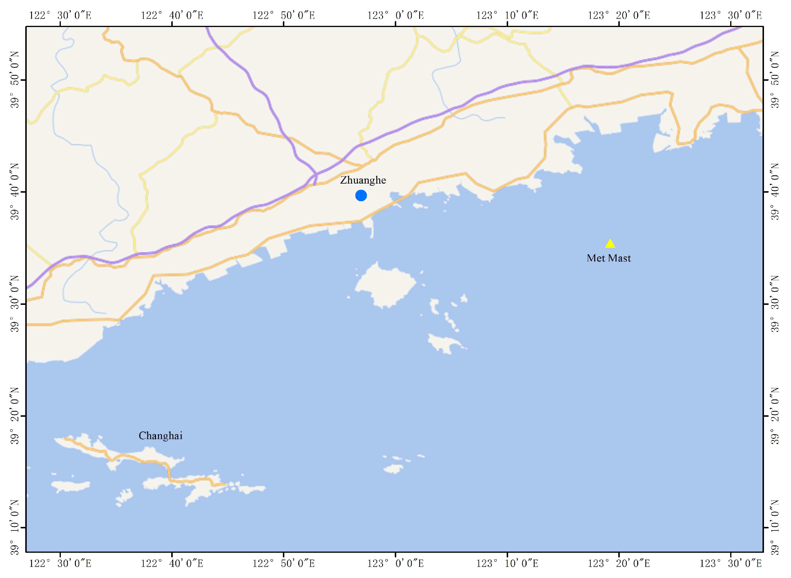
Figure 2.
Distribution of atmospheric stability and temperature difference at different heights. (a) 20m. (b)50m. (c)80m. (d)100m. The monthly variations of the occurrence frequency for stable (green), neutral (blue), and unstable (orange) .
Figure 2.
Distribution of atmospheric stability and temperature difference at different heights. (a) 20m. (b)50m. (c)80m. (d)100m. The monthly variations of the occurrence frequency for stable (green), neutral (blue), and unstable (orange) .
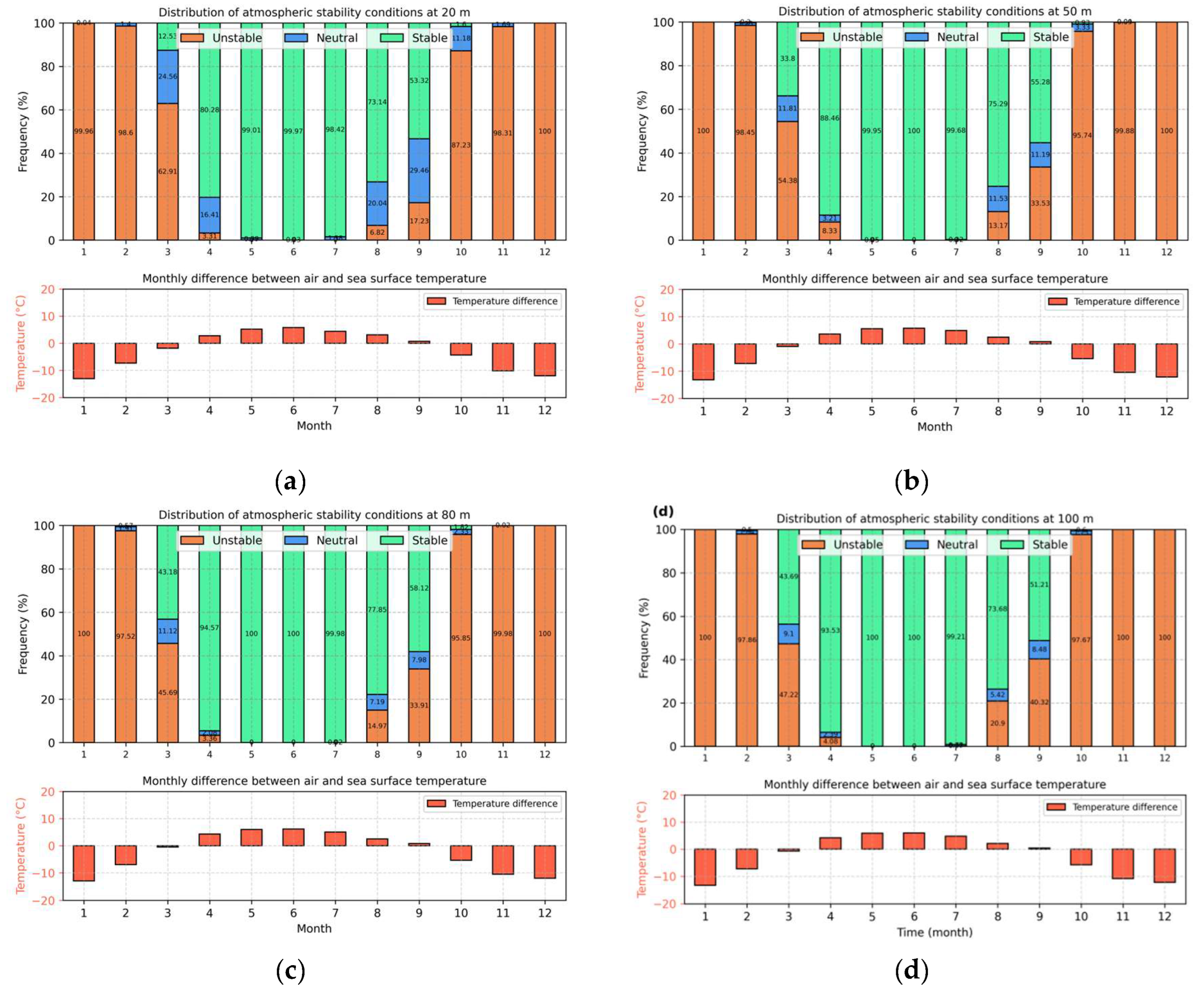
Figure 3.
Diurnal distribution of atmospheric stability conditions for different month. (a) March.(b)April.(c) August.(d) September.
Figure 3.
Diurnal distribution of atmospheric stability conditions for different month. (a) March.(b)April.(c) August.(d) September.
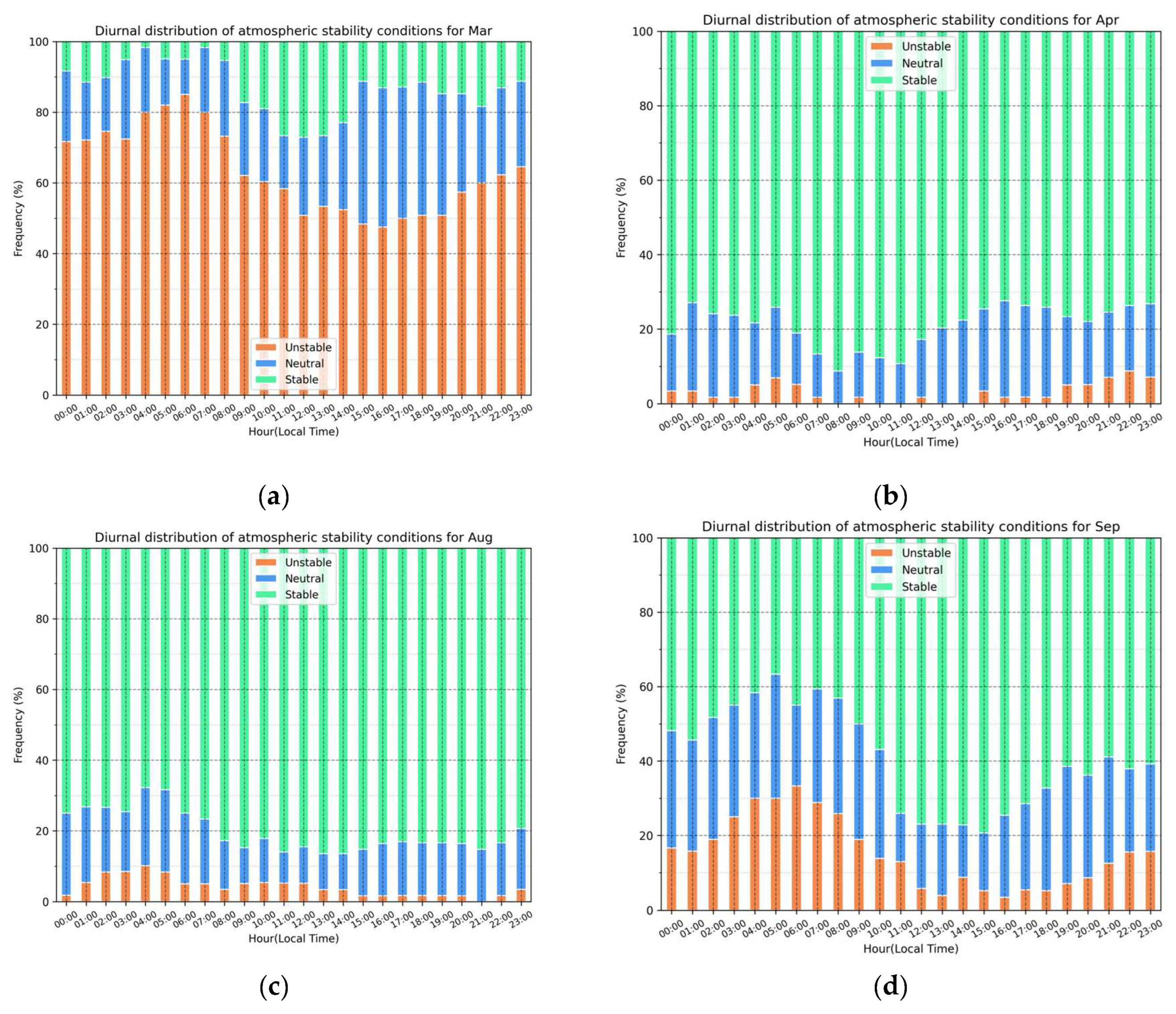
Figure 4.
Atmospheric stability by wind speed.
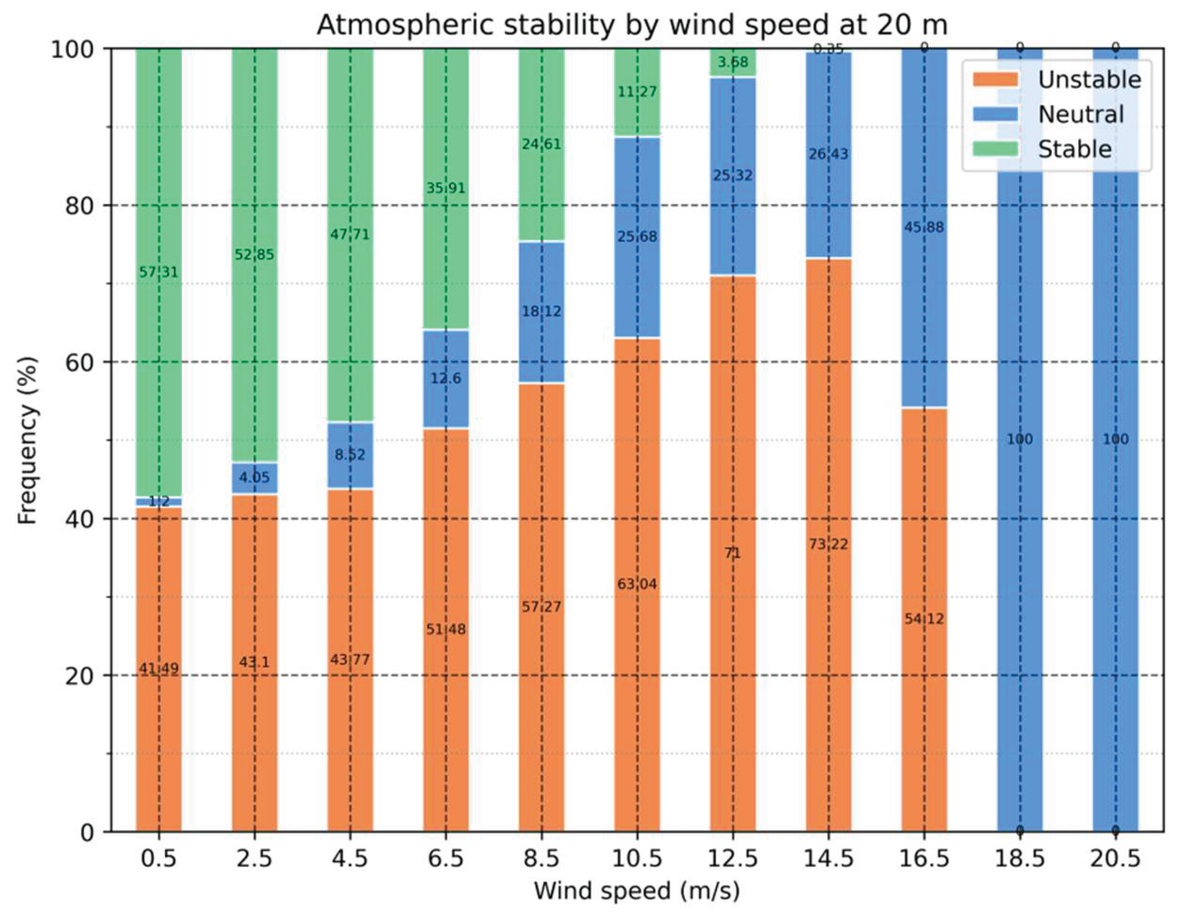
Figure 5.
Frequency distribution of atmospheric stability by wind direction. (a) Spring (Mar-Apr). (b) Summer (May to July). (c) Autumn (Aug-Sept). (d) Winter (Jua- Feb, Oct-Feb).
Figure 5.
Frequency distribution of atmospheric stability by wind direction. (a) Spring (Mar-Apr). (b) Summer (May to July). (c) Autumn (Aug-Sept). (d) Winter (Jua- Feb, Oct-Feb).
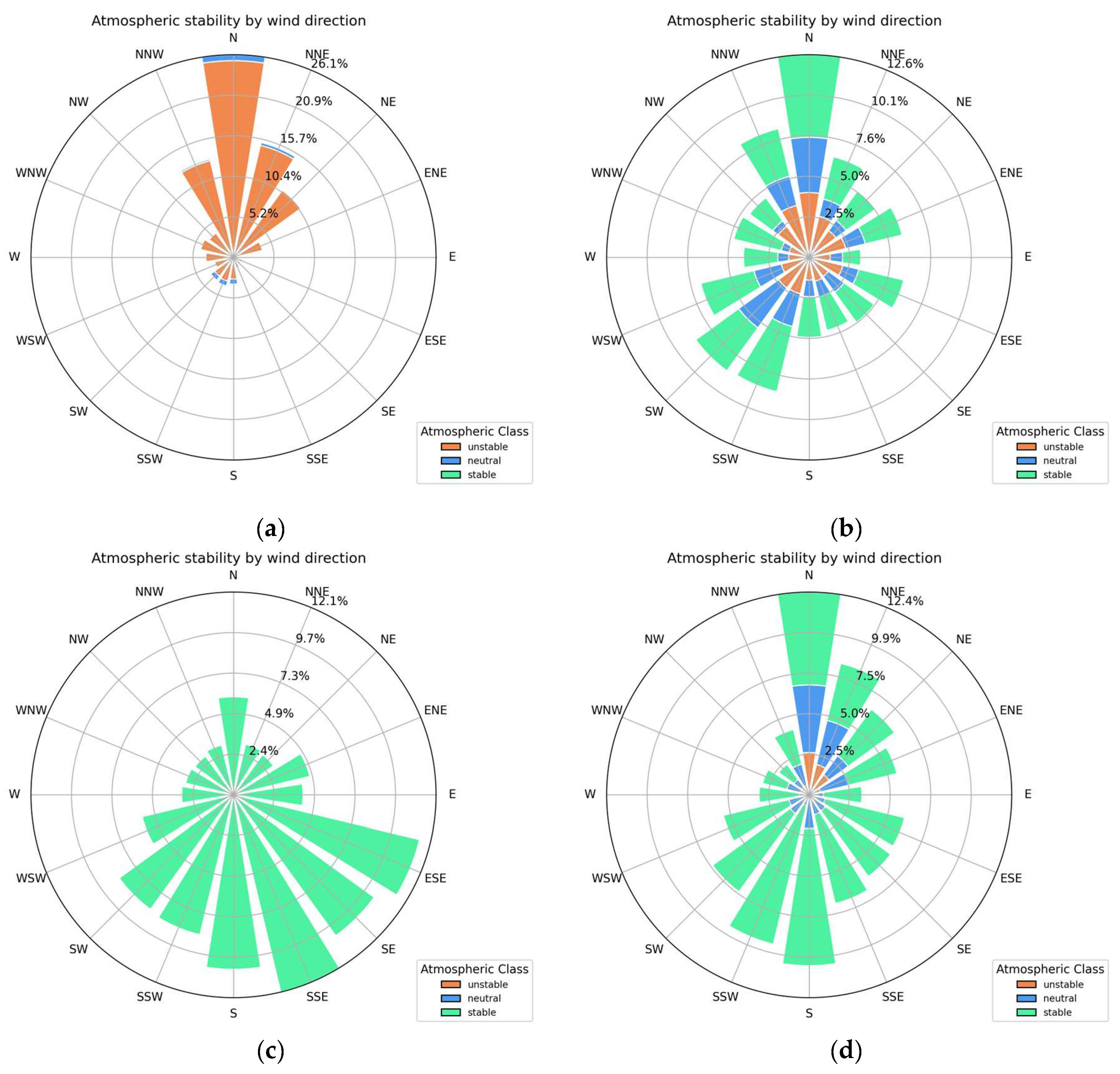
Figure 6.
Diurnal variation of wind shear coefficient α under three atmospheric conditions. (a) unstable. (b) stable. (c) neutral.
Figure 6.
Diurnal variation of wind shear coefficient α under three atmospheric conditions. (a) unstable. (b) stable. (c) neutral.
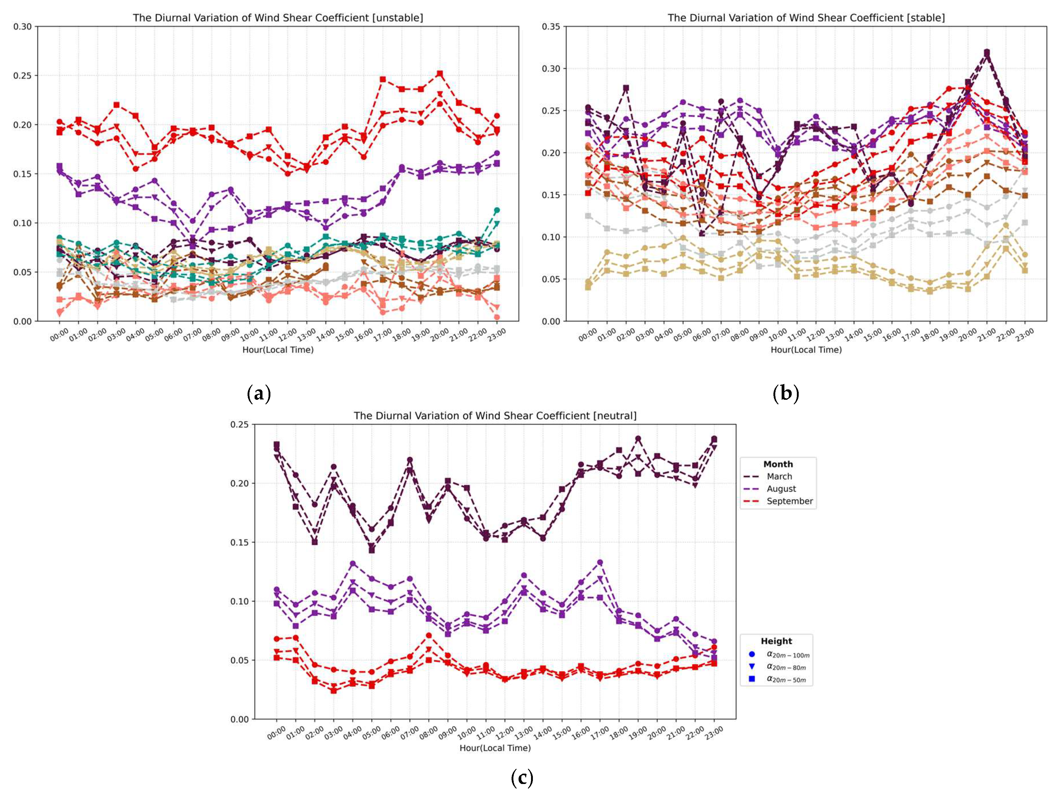

Table 1.
Instruments information of Meteorological mast.
| Parameter | Instrument | Company | Heights(m) | Sample |
| wind speed | cup anemometer class 1 | NRG | 20,50,80,100 | 10 min |
| wind direction | wind vane | NRG | 20,50,80,100 | 10 min |
| wind speed | cup windsenP2546A | Risø | 20,50,80,100 | 10 min |
| wind direction | wind vane | Risø | 20,50,80,100 | 10 min |
| air temperature | temperature sensor 110s | NRG | 20,50,80,100 | 10 min |
Table 2.
The classification of atmospheric stability.
| Parameter | Range | Atmospheric stability classes |
| unstable | ||
| neutral | ||
| stable |
Table 3.
The annual probability with different atmospheric conditions.
| Heights | 20m | 50m | 80m | 100m |
| unstable | 43.18% | 46.05% | 47.93% | 46.79% |
| neutral | 8.93% | 3.58% | 2.73% | 2.46% |
| stable | 47.89% | 50.37% | 49.34% | 50.75% |
Table 4.
Wind shear coefficients (WSCs) calculated at different heights.
| Wind shear coefficient between heights | Symbol |
| 20m and 50m | |
| 20m and 80m | |
| 20m and 100m |
Disclaimer/Publisher’s Note: The statements, opinions and data contained in all publications are solely those of the individual author(s) and contributor(s) and not of MDPI and/or the editor(s). MDPI and/or the editor(s) disclaim responsibility for any injury to people or property resulting from any ideas, methods, instructions or products referred to in the content. |
© 2026 by the authors. Licensee MDPI, Basel, Switzerland. This article is an open access article distributed under the terms and conditions of the Creative Commons Attribution (CC BY) license (http://creativecommons.org/licenses/by/4.0/).
Copyright: This open access article is published under a Creative Commons CC BY 4.0 license, which permit the free download, distribution, and reuse, provided that the author and preprint are cited in any reuse.


