

Submitted:
21 July 2026
Posted:
22 July 2026
Read the latest preprint version here
Abstract
Quantum-kernel methods encode a dataset’s geometry in a Gram matrix, so learning claims on hardware kernels assume the intended geometry survives execution. We measure that survival for one frozen four-qubit ZZ feature map kernel on N = 24 real indoor air-quality windows, reconstructed on ibm_fez (1024 shots per circuit) under baseline, dynamical decoupling alone, and gate twirling alone, each a single non-interleaved job. Every configuration returned a complete, finite, positive-semidefinite Gram matrix and preserved the centered statevector geometry to a substantial but incomplete descriptive degree (full-matrix centered kernel alignment, CKA, 0.933–0.989). Gate twirling was most faithful on every reported geometry axis, with the only jackknife-resolved improvement over baseline (persisted Spearman, mean absolute error, and full-matrix CKA diagnostics); dynamical decoupling alone was not separated from baseline at the frozen-window scale. Residual hardware distortion, not finite sampling, dominates the discrepancy. Yet fidelity and label alignment were reversed: the most faithful configuration had the lowest centered kernel–target alignment, which sits at or below label-permutation references for statevector and hardware alike. We read the small hardware uplift as a normalization property of the non-affine distortion, not captured signal. These are descriptive results for single jobs on one backend, not causal mitigation-efficacy estimates; no quantum-advantage, hardware-classifier-superiority, or forecasting claim is made. Implementation fidelity and task relevance are distinct axes; hardware quantum machine-learning studies should report both.
Keywords:
quantum kernel
; ZZ feature map
; quantum machine learning
; IBM Quantum hardware
; dynamical decoupling
; gate twirling
; centered kernel alignment
; kernel–target alignment
; indoor air quality
1. Introduction
1.1. Background and Motivation
Indoor air-quality (IAQ) monitoring increasingly relies on networks of low-cost sensors whose multivariate streams are noisy, incomplete, and partially redundant [1,2]. Sensor drift, missing values, duplicate or colocated behavior, and weakly separated event labels make this a demanding setting for any similarity-based learning method, and therefore a useful real-world testbed for nonlinear kernels. The broader monitoring project that motivates this work is concerned with redundancy- and missingness-aware (RMA) sensor modeling. The present hardware experiment, however, is deliberately restricted to a single fixed four-qubit ZZ feature map (ZZ4) and does not execute any RMA kernel on quantum hardware; RMA is named here only to situate the experiment within the larger project, not as an object of the present study.
A quantum feature map embeds a classical input x into a quantum state,
and the associated quantum kernel measures similarity through a squared overlap,
so that the kernel (Gram) matrix encodes a learned geometry of the dataset [3–5]. Because every downstream kernel method sees the data only through this matrix, the fidelity of the matrix itself is a precondition for any learning claim built on it.
On near-term hardware, finite sampling and device noise distort these overlaps. Both theory and experiment indicate that noise drives kernel entries toward a common background, flattening the matrix and removing the feature map’s intended geometric structure [6–8]. If hardware noise substantially distorts the kernel geometry, then conclusions about quantum machine learning (QML) drawn from that hardware kernel are premature.
We therefore adopt a focused stance. This paper does not ask whether a quantum computer improves indoor air-quality prediction. It asks the logically prior question: can the statevector ZZ4 kernel geometry be reconstructed on real IBM Quantum hardware with interpretable, bounded distortion? Establishing that a kernel survives execution — and characterizing how it fails to — is a prerequisite for, and distinct from, any later claim of quantum advantage [9–12].
1.2. Related Work
Quantum kernel methods. The ZZ-type feature map and the squared-overlap quantum kernel used here originate in supervised learning with quantum-enhanced feature spaces on superconducting hardware [3], with the feature-Hilbert-space interpretation of quantum encodings made explicit by Schuld and Killoran [4] and later sharpened into the statement that supervised quantum models are kernel methods [5]. Quantum kernels are estimated either by fidelity (compute–uncompute) circuits or by projected variants; large benchmarking studies show that their behavior hinges on encoding, bandwidth, and concentration rather than on the mere use of a quantum device [13], and the expressivity and limits of embedding (fidelity) kernels are now reasonably well characterized [14]. A recurring theme is that a large quantum feature space does not by itself help: without the right inductive bias, generalization can degrade [15], kernel values can concentrate exponentially toward a constant and wash out discriminative structure [6], and access to sufficient data can make classical models competitive with quantum ones [12]. These results motivate treating the statevector kernel — not the hardware kernel — as the intended geometry, and asking how much of it survives execution.
Quantum machine learning on NISQ hardware. Moving a quantum kernel from a noiseless simulator to a noisy intermediate-scale quantum (NISQ) device is nontrivial. Flagship demonstrations have run quantum-kernel classifiers on superconducting processors at the 17–27-qubit scale [9,11], and embedding kernels have been trained and assessed directly on noisy hardware [10]. Yet finite-shot estimation, hardware noise, and compilation all degrade the estimated kernel: kernel-advantage arguments weaken with large datasets, few shots, and high noise [6,8], decoherence reduces the effective rank of the kernel ([7], Figure 6), and the realized benefit of techniques such as dynamical decoupling depends jointly on the device and on transpilation and circuit-design choices [16]. Readout and other circuit-level errors are a further source of bias, addressable by dedicated readout-error mitigation [17,18] and surveyed alongside other approaches in the error-mitigation literature [19]. The closest hardware-fidelity neighbor to the present work validates a quantum-kernel support vector machine on the same backend family and reports high statevector-to-hardware fidelity correlation together with overly flat, concentrated quantum eigenspectra relative to a radial-basis-function (RBF) kernel [20] (preprint). Broader overviews place trainability and noise at the center of QML’s open problems [21].
Error mitigation and execution configurations. The three execution configurations compared in this work — baseline, dynamical decoupling, and gate twirling — correspond to standard mitigation strategies that can be selected at runtime. Dynamical decoupling suppresses idle decoherence through pulse sequences [22], with modern device-level performance characterized for superconducting qubits [23]. Gate (Pauli) twirling, or randomized compiling, tailors coherent error into stochastic noise that behaves more predictably [24]. These sit within a broader toolbox that includes zero-noise extrapolation and probabilistic error cancellation [25], reviewed comprehensively elsewhere [19]. Crucially, mitigation reduces error, but this alone is not evidence of predictive benefit. Studies that combine several mitigation techniques and evaluate them by downstream classifier accuracy [26] answer a different question from the one posed here, where each configuration is executed in isolation and judged by kernel-geometry survival rather than by accuracy [8,19].
Kernel alignment and geometry metrics. We measure kernel-geometry survival with representation-similarity and alignment tools. Centered kernel alignment (CKA) compares two kernels’ centered geometries [27]; centered (Cortes-type) kernel–target alignment (KTA) compares a kernel’s centered geometry with a label Gram matrix [28], the same family of alignment measures used to assess and train quantum embedding kernels on hardware [10]. Spectral structure is summarized by the entropy-based effective rank [29], which connects to the effective kernel rank under noise [7], and positive-semidefinite (PSD) behavior is checked against the nearest-PSD projection [30]. Both CKA and centered KTA are invariant to affine (scale-and-shift) changes of a kernel, so a purely depolarizing-type contraction cannot move them. This sets up the central tension of the study: alignment with the statevector geometry (CKA) and alignment with the labels (KTA) need not move in the same direction. A recent kernel-level comparison reports that depolarizing noise increases quantum–classical CKA, reading near-term hardware kernels as structurally closer to an RBF kernel than noiseless simulations suggest [31] (preprint, small datasets); we instead read our data through a non-affine distortion whose alignment uplift is normalization-associated (compression of the centered kernel norm), and develop that reading in the Discussion (Section 4.4).
Indoor air-quality and sensor data. Finally, the data are real. Low-cost air-quality sensing has matured substantially [1], but inter-unit variability, drift, and noise remain well documented [2]. We do not use this setting as an environmental-prediction benchmark. Instead, we treat the duplicate-sensor records as real but imperfect data on which to stress-test hardware-kernel reconstruction.
1.3. Research Gap and Contributions
Across this literature, two facts coexist. First, quantum kernels have been executed on real hardware, and concentration theory explains why noise should flatten them [6,7,9,11]. Second, the standard mitigation strategies, such as dynamical decoupling and twirling, and the standard geometry diagnostics, such as CKA, KTA, effective rank, and nearest-PSD projection, are each individually well established [22,24,27–30]. What is comparatively underexplored is their combination on a single, fixed kernel: a controlled, statevector-referenced measurement of how much of one frozen kernel’s geometry survives reconstruction on a real device, compared across distinct execution configurations and decomposed against an explicit finite-shot reference scale. The nearest hardware-fidelity study reports fidelity correlation and spectral flatness but does not isolate per-configuration centered-geometry survival or the alignment tension [20]; studies that apply mitigations jointly judge them by classifier accuracy rather than by kernel geometry [26]; and the finite-shot sampling scale of compute–uncompute kernels, although formalized [8,32], is rarely used as an explicit reference against which residual hardware distortion is measured.
To address this gap, we:
- 1.
- execute a fixed four-qubit ZZ4 quantum kernel on real IBM Quantum hardware, using a frozen indoor air-quality subset of observation windows;
- 2.
- compare three execution configurations — baseline, dynamical decoupling, and gate twirling — each submitted as a single non-interleaved job;
- 3.
- analyze hardware-versus-statevector kernel survival by combining rank-order, linear, entrywise-error, alignment (CKA and KTA), spectral (effective rank), and PSD diagnostics;
- 4.
- report a central CKA/KTA tension, in which the configuration with the best geometric fidelity to the statevector kernel does not maximize label alignment; and
- 5.
- quantify how much of the observed off-diagonal root-mean-squared error (RMSE) can be attributed to a conservative finite-shot sampling scale.
These contributions are diagnostic. The single-job execution design supports descriptive comparison of the three configurations on this backend but not a causal estimate of mitigation efficacy, and the fixed subset supports geometry-survival claims rather than predictive ones (Section 1.4).
1.4. Research Questions and Scope
This work is a fixed-subset hardware-kernel diagnostic pilot. It characterizes statevector-to-hardware geometry survival and distortion for one fixed ZZ4 kernel under three pre-authorized execution configurations on a single backend (ibm_fez), at 1024 shots per circuit. This frozen execution stage is designated Wave 1 in the project’s decision record, and the public reproducibility package and release tag retain that name. This study does not estimate general mitigation efficacy and does not test indoor air-quality forecasting accuracy, quantum advantage, or hardware classifier superiority. Throughout, “survival” is reported as a continuous, multi-metric description; no binary pass/fail survival threshold was pre-specified, and the directional expectations E1–E4 that accompany the research questions are reproduced verbatim, with their provenance status, in Section 2.13. We address four research questions.
RQ1 — geometry survival. To what extent is the geometry of the fixed four-qubit ZZ4 statevector kernel preserved when reconstructed on IBM Quantum hardware for the frozen subset, as measured by rank-order (Spearman), linear (Pearson), entrywise (mean, root-mean-squared, and maximum absolute error), and centered full-matrix (CKA) agreement with the statevector reference?
RQ2 — configuration differences. What descriptive differences in centered-geometry preservation and off-diagonal entrywise distortion are observed among the three configurations — baseline, dynamical decoupling alone, and gate twirling alone — each submitted as a single non-interleaved job?
RQ3 — finite-shot reference scale. How does the observed off-diagonal hardware-versus-statevector RMSE compare with a conservative global and an entry-resolved finite-shot reference scale, and does residual hardware distortion dominate the discrepancy under the Wave 1 reconstruction?
RQ4 — label alignment as a distortion diagnostic. Does the intended ZZ4 statevector kernel align with the frozen event-onset labels beyond a random-label permutation reference on this subset, and should any CKA/KTA divergence be interpreted as a distortion diagnostic rather than as evidence of supervised predictive improvement?
Throughout, we keep statevector, noisy-simulation, and hardware quantities distinct, and we treat all alignment and spectral changes as diagnostics of hardware distortion. We do not claim quantum advantage, hardware classifier superiority, or improved IAQ forecasting. The term “quantum advantage” appears here only to mark what this study does not test. The rest of the paper is organized as follows. Section 2 specifies the dataset, the ZZ4 feature map, the frozen subset, the IBM Quantum hardware protocol, and the survival and distortion metrics. Section 3 reports the reconstruction, the distortion metrics, the CKA/KTA tension, and the finite-shot reference-scale decomposition. Section 4 discusses the implications for reporting quantum machine-learning results on hardware, Section 5 consolidates the binding limitations, and Section 6 concludes.
2. Materials and Methods
2.1. Dataset and Prediction Context
We used real indoor air-quality duplicate-sensor monitoring data organized as a forecasting dataset with a 30-minute window stride and a one-hour prediction horizon. The prediction task was binary event-onset forecasting: for each eligible time window, the response variable indicated whether a new air-quality event started within the next hour. In the repository, this target is recorded as event_onset_next_1h; in the frozen hardware subset, the corresponding column is y_event_onset_next_1h. Rows were eligible when this onset target was non-missing and the upstream future-label quality flag label_valid_1h was true. This flag is defined in the parent dataset builder and is not carried into the frozen-subset table (whose retained target column is y_event_onset_next_1h). In the parent dataset builder, event_onset_next_1h is assigned only to windows with event_now = 0. Together, the two eligibility conditions therefore exclude windows with an already active event and windows with invalid or boundary-purged future labels.
The parent event-onset dataset used a time-aware train/validation/external-test split. For the event_onset_next_1h target with the compact F_quantum_4 representation, the repository records 1,163 valid training rows, 471 validation rows, and 931 external-test rows, with 237, 124, and 213 positive cases, respectively. These full-split counts are reported only to define the prediction context; the quantum-hardware analysis described here was restricted to a pre-authorized frozen subset, described separately below.
The associated statevector reference metadata records the frozen subset as 16 training observation windows and 8 test observation windows. For this subset, the repository records 300 unique unordered kernel evaluations, including diagonal terms and 276 unique off-diagonal pairs. These counts define the hardware-kernel evaluation scope for the ZZ4 pilot.
The feature set was F_quantum_4, comprising four one-hour pollutant summary features: pm25_mean_last_1h, pm10_mean_last_1h, hcho_mean_last_1h, and tvoc_mean_last_1h. These inputs were processed under the repository’s train-only preprocessing policy: missing values were imputed from the training data, features were min-max scaled to , and values outside the training range in later splits were clipped.
The kernel used for the frozen subset was ZZ4, defined as a four-feature ZZ feature map applied to the scaled F_quantum_4 inputs. The statevector reference kernel was the squared-overlap quantum kernel [3,4], [11]. Accordingly, this experiment was framed as a statevector-to-hardware kernel-geometry distortion and survival analysis, not as a test of quantum advantage or hardware classifier superiority [8].
Reproducibility and artifact grounding. The public Wave 1 repository is available at a fixed commit (github.com/rsipakov/iaq-quantum-kernel-wave1-reproducibility, commit 6d14bca984486509b40850372f373c3499843dbc, release tag v1.2-wave1-manuscript); a permanent archival snapshot of this release is deposited at Zenodo (DOI 10.5281/zenodo.21332398). The repository is an artifact-level reproducibility package for the frozen ZZ4 hardware analysis. It contains the frozen subset, the statevector reference, the raw and reconstructed IBM Quantum result artifacts, and the audit and analysis scripts that reproduce the reported reconstruction, distortion, uncertainty, and shot-noise diagnostics. It does not rebuild the full upstream IAQ dataset and does not re-submit IBM Quantum jobs. The original numbered execution scripts retained in the repository are archival records from the source execution environment. They are not the supported reproduction path for the flat public package. Supplementary Note S1 provides the consolidated section-to-artifact map, including file paths, scripts, and checksum coverage for the Methods Sections 2.1–2.13 and the per-section artifact grounding for the Results Sections 3.1–3.7.
2.2. Frozen Subset
We selected a subset of observation windows from the duplicate-sensor indoor air-quality monitoring dataset and froze it before IBM hardware execution was authorized. Each window provides one scaled four-dimensional F_quantum_4 feature vector as input to the ZZ4 kernel. The subset, inclusion criteria, and acceptance thresholds used for compile-gate and stability checks were pre-specified and recorded in the freeze and execution artifacts; they were not modified after hardware results were obtained.
At the row level, the frozen subset comprises 16 training and 8 test windows drawn from the parent time-aware splits, balanced by construction in the signed labels (12 event-onset and 12 non-onset windows; 8 of 16 training and 4 of 8 test windows positive). The 24 windows span 2024-12-22 to 2026-04-20, with a median spacing of days between consecutive windows. Only two consecutive pairs lie 30 minutes apart, so at most two pairs of one-hour summary windows overlap in raw data. The full per-window ledger (row order, window end, split, and label) is reported in Supplementary Table S2.9. Dated, checksum-locked artifacts precede job creation (2026-05-09 08:42:04 UTC). The subset-stability record (05:35 UTC) set informal acceptance bands for the statevector effective rank () and uncentered alignment (), logged that both bands held across seven permutation seeds, and recorded that no alternative balanced subsets were evaluated. The scope-lock and authorization records (08:33 UTC) fixed the subset, kernel, feature set, and regimes. The public package records the resulting frozen rows and these dated freeze artifacts; it does not include the drawing procedure’s candidate-pool enumeration or selection seed.
Within the current pre-authorized scope, the frozen subset is not an adjustable analysis input. We did not add, remove, replace, reorder, or reweight any observation window after hardware execution authorization. This restriction applies in all cases: missing data, intermediate model behavior, hardware results, kernel distortion, diagnostic outcomes, reviewer preference, or downstream performance.
The current Wave 1 decision record states STOP_AFTER_WAVE1_REPORT_RESULTS. It allows only the frozen subset, blocks subset changes and threshold relaxation within the v9 scope, and requires a new decision record for any Wave 2 execution. The results reported here, therefore, apply only to this pre-authorized ZZ4 hardware pilot.
Extensions to additional regimes, sentinel-only follow-up runs, or larger subsets fall outside the present scope unless authorized by a new decision record, and may not retroactively alter the frozen subset, thresholds, or claims.
2.3. ZZ4 Quantum Feature Map
The quantum-kernel component of the hardware pilot used a fixed four-dimensional, second-order Pauli-Z (ZZ) feature map, denoted ZZ4. Its input was the train-only scaled F_quantum_4 vector introduced above,
whose four components correspond, in this order, to pm25_mean_last_1h, pm10_mean_last_1h, hcho_mean_last_1h and tvoc_mean_last_1h. The tilde emphasizes that these are not raw pollutant readings but imputed, min-max scaled, and clipped values produced under the training-split preprocessing policy. No reliability, momentum, missingness, lag, or metadata features were supplied to ZZ4 in the hardware run.
Circuit definition. ZZ4 was implemented as Qiskit’s ZZFeatureMap on four qubits, one per feature. For an input vector the circuit prepares
where consists of two repetitions, each a layer of Hadamard gates followed by a data-encoding layer of single- and two-qubit Z rotations. In the Qiskit ZZFeatureMap convention used here [3], the data map combines first-order terms on qubit k with second-order terms on coupled pairs , and the implementation used the default Qiskit scaling, . Entanglement is linear (nearest-neighbor): only the adjacent feature qubits carry ZZ couplings, so the map is not all-to-all. The configuration (feature dimension 4, linear entanglement, two repetitions, ) was fixed before hardware execution and was not re-tuned after observing statevector or IBM hardware outputs. The same configuration defines both the statevector reference and the hardware fidelity circuits; the hardware kernels are therefore empirical reconstructions of one fixed geometry, not separately parameterized kernels.
Statevector reference. The statevector reference kernel was the exact squared-fidelity kernel induced by this map,
For the frozen subset, this reference was computed for the 16 training windows, the 8 test windows, and the combined () set; the combined matrix served as the geometry baseline for the hardware distortion analysis. By construction, the statevector diagonal equals unity up to numerical precision. The hardware diagonal was retained as measured rather than forced to one. In the reported compiled artifacts, diagonal compute–uncompute circuits reduce to terminal measurement-only circuits; therefore, these entries primarily reflect preparation/reset, readout, and finite-shot effects rather than feature-map gate errors.
Hardware estimator. Each hardware kernel entry was estimated with a direct (compute–uncompute) fidelity circuit. For each pair the operator
was applied to and all four qubits were measured. In the noiseless limit, the probability of the all-zero outcome equals the squared overlap,
On IBM Quantum hardware, this probability was estimated from SamplerV2 counts by the finite-shot estimator
where denotes the pre-authorized execution regime, is the observed all-zero count and the observed shot count for the corresponding circuit. In an idealized fully depolarized four-qubit output distribution, the all-zero probability would approach the uniform floor . Real hardware noise and finite-shot sampling do not follow this model exactly, but the limit illustrates why compute–uncompute kernel entries can develop a nonzero background and why noise drives measured overlaps toward a common value [6], [7]. We therefore interpret effective-rank and alignment changes as diagnostics of hardware distortion rather than as evidence of improved classification geometry.
The reported artifacts used a budget-safe execution with 1024 submitted shots per circuit for H0, H1, and H2, rather than the originally planned 4096. This shot count affects the statistical precision of but not the definition of the ZZ4 map or of the statevector reference kernel.
Matrix assembly. The frozen subset contains observation windows, so the unordered pair inventory, including diagonal pairs, contains ZZ4 kernel evaluations. These 300 pairs were evaluated in each of the three regimes, yielding 900 circuit–regime configurations. These are not 900 distinct logical circuit bodies: the regimes differ only in Sampler-level runtime options applied at execution time (Section 2.5). In the executed runs, each unordered pair with was measured exactly once, with no directed or replicated observations. Symmetrization therefore reduced to mirroring the measured upper triangle, , and the averaging rule for replicated entries was not used. Retrieved SamplerV2 outputs were mapped back to the preserved circuit index, converted to all-zero probabilities, and assembled into one hardware kernel matrix per regime. The diagonal was not forced to one; it followed the measured-diagonal policy. We applied positive-semidefinite projection only as a diagnostic calculation and kept the uncorrected minimum eigenvalue in the metadata.
We thus treated the ZZ4 hardware kernels as empirical reconstructions of the same feature-map geometry defined by the statevector reference, not as separate learned kernels. The analysis endpoint was kernel survival and hardware-induced geometric distortion relative to . Accordingly, the ZZ4 pilot design does not support claims of quantum advantage, hardware classifier superiority, or readiness of the separate RMA feature-map family for hardware execution.
2.4. Pair Inventory
The pair inventory is the fixed, row-level coordinate ledger that determines which entries of the frozen-subset kernel were evaluated and how each entry was traced back to its circuit and samples. It served as a coordinate lock rather than as an analysis result: the off-diagonal pair count (276) and the total including the diagonal (300) follow from the frozen-subset size and are stated in Sections 2.1 and 2.3, so they are not re-derived here. The enumeration is the complete upper triangle
traversed in a fixed order from to .
Each row carries a stable pair identifier, an integer pair order, the two kernel coordinates , the corresponding frozen-subset sample identifiers, a diagonal/off-diagonal type label, a symmetry-mirror flag, a full-kernel inclusion flag, and a sentinel-pair flag. Off-diagonal rows are tagged as mirrorable and diagonal rows as non-mirrorable, consistent with the symmetrization of Section 2.3. The inclusion flag is set for all 300 rows. The sentinel-pair flag is unset for all 300 rows, so no sentinel pairs were designated in this pilot, in line with the decision-record scope of Section 2.2. Sample references are opaque row identifiers, and the inventory’s split- and target-label fields are present in the schema but left unpopulated, so no split membership or class label is attached to any pair row.
This schema allowed the pair list to be audited independently of the circuit-construction and retrieval steps. The downstream circuit and kernel artifacts reference pair identifiers instead of re-deriving coordinates, which avoids ambiguity in row order, diagonal handling, and pair inclusion. Because the coordinate set was exhaustive for the frozen subset and carried no label or split information, pair inclusion was label-blind by construction — no class label, split membership, hardware result, or downstream distortion statistic could determine whether a pair entered the full-kernel inventory.
2.5. IBM Quantum Hardware Protocol
Backend and primitive. The pilot was executed on the IBM Quantum backend ibm_fez, selected before submission from the pre-authorized candidate set {ibm_fez, ibm_marrakesh, ibm_kingston} under the rule that the package-selected backend is retained unless the live-metadata gate fails. A live snapshot taken immediately before submission identified ibm_fez as a 156-qubit, version-2 device reported operational, and the backend passed the live-metadata gate with no scope drift detected. The snapshot captured an operation set including cz, rz, sx, and x, together with a sampling period . The compiled circuits used cz as the recorded two-qubit operation after transpilation. Circuits were executed with the SamplerV2 sampler primitive of the Qiskit Runtime primitives framework [33] (Qiskit 2.4.1, qiskit-ibm-runtime 0.46.1) in backend job mode rather than in a Runtime session, so no session identifier is recorded for the three jobs.
Circuit construction and compilation. The submitted PUBs were the compute–uncompute fidelity circuits defined in Section 2.3. The 300 pair-dependent logical circuit bodies were shared across regimes. The 900 inventory rows represent circuit–regime configurations, not 900 independently designed logical circuits, because dynamical decoupling and twirling are applied by the primitive at execution time rather than embedded in the submitted circuits. We confirmed the compile metrics by transpiling to ibm_fez before submission. The post-transpilation values are a maximum compiled depth of 102, a maximum two-qubit-gate count of 22, and at most four active data qubits, with the circuits laid out on the 156-qubit device. The resource gate passed for every configuration. The frozen metadata artifacts store these resource metrics, the operation set, the sampling period, and the SDK versions. They do not include the physical-qubit layout, the transpilation seed, or a contemporaneous per-qubit calibration table (the archival submission script records optimization_level=1). The archived circuit file (circuits/zz4_wave1_circuits.qpy) preserves the 900 logical pair circuits rather than the compiled ISA circuits, so those execution-level details are recoverable only from the IBM Quantum job records (job identifiers in Section 3.1), where account access allows.
Mitigation regimes. Three Sampler-level regimes were defined. The per-regime runtime-option records were SHA-256 locked, and the digests match across the runtime-options, backend-snapshot, and job-manifest artifacts. Regime H0 is the unmitigated baseline (dynamical decoupling off; gate and measurement twirling off). Regime H1 enables dynamical decoupling only [22], using an XX sequence with alap scheduling and middle extra-slack distribution, and no twirling. Regime H2 enables gate (Pauli) twirling only [24], with dynamical decoupling and measurement twirling off and the active-accum accumulation strategy. The auto randomization setting resolved at execution to 16 randomizations per circuit for all H2 PUBs. This pilot did not combine dynamical decoupling and gate twirling.
Shot budget. The locked plan specified 4096 shots per circuit. The reported execution used a budget-safe override of 1024 submitted shots per circuit for every regime, which affects only finite-shot precision and not the definitions of Section 2.3. The retrieved counts confirm exactly 1024 observed shots per circuit in all three regimes. For the twirled regime H2, the raw result metadata records 16 randomizations and 1024 observed shots per PUB (64 shots per randomization if allocated evenly). The analysis used the pooled 1024-shot count and did not model between-randomization variability. As a finite-shot reference, the per-entry binomial plug-in shot-noise scale is
This is a shot-noise scale, not a hardware-noise model, and it was not used as an uncertainty model in the present analysis. For H2, the shots are pooled across randomizations, so this expression does not capture between-randomization variability. Per-randomization counts were not persisted and cannot be recovered from the pooled counts, so the H2 dispersion across randomizations remains unquantified beyond this pooled binomial scale.
Submission and retrieval. We submitted one backend-mode job per regime, each covering all 300 pair circuits: d7vf6n3ack5s73bfc0eg (H0), d7vf8ocinasc738u1bhg (H1), and d7vfbsfmrars73d84u20 (H2). All three jobs completed with status DONE. The retrieval manifest records 300 PUB results per regime with no retrieval failure: 900 retrieved circuit–regime configurations in total.
Persisted artifacts. For each PUB, the raw result artifacts preserve the full count dictionary, the observed shot count, the regime label, the circuit-inventory and pair identifiers, the pair-inventory row, the kernel coordinates , and, for H2, the realized randomization count. The derived long-form table records, per regime and pair, the all-zero bit string, the all-zero count, the observed shots, and the raw finite-shot kernel value; the kernel manifest records one complete matrix per regime with no missing entries, the measured-diagonal policy, and positive-semidefinite metadata recorded for diagnostics only. The protocol thus produced three empirical ZZ4 reconstructions (H0, H1, and H2) of one fixed feature-map geometry. No RMA-family execution, Wave 2 execution, subset modification, or threshold relaxation was part of this protocol.
2.6. Execution Configurations
The persisted artifacts label the three Sampler-level regimes of Section 2.5 as H0, H1, and H2. Because the artifact label H0 is easily confused with the conventional null-hypothesis symbol , the manuscript refers to these same regimes as manuscript-level execution configurations M0, M1, and M2. The configurations are not redefined here: M0, M1, and M2 denote exactly the baseline, dynamical-decoupling, and gate-twirling regimes specified in Section 2.5, with no change to circuits, jobs, kernels, shots, preprocessing, or analysis.

Table 1.
Execution-configuration alias map.
| Configuration | Artifact label | Description |
|---|---|---|
| M0 | H0 | Baseline Sampler configuration |
| M1 | H1 | Dynamical-decoupling configuration |
| M2 | H2 | Gate-twirling configuration |
Writing a for the alias map,
Thus, for every frozen-subset pair and every manuscript configuration ,
The map is for the three executed regimes only. No combined dynamical-decoupling-plus-twirling configuration was executed, and the reserved scope-artifact labels H3–H5 were not executed and are outside the present analysis.
The alias applies only to the manuscript and documentation. Persisted reconstruction and analysis artifacts (file names, JSON fields, CSV regime columns, raw-count records, reconstructed kernel matrices, job manifests, and checksums) remain keyed by H0, H1, and H2. Because the per-regime runtime-option records are SHA-256 locked as part of the hardware protocol (Section 2.5), the artifact labels form a fixed substrate that the manuscript alias cannot modify. The relabeling therefore cannot affect reproduction and carries no inferential meaning. It is neither a null/alternative-hypothesis convention nor a model-selection step.
2.7. Kernel Reconstruction
Kernel reconstruction took place after IBM Quantum job retrieval and left the frozen subset, the pair inventory, the execution configurations, and the circuit definitions unchanged. For each artifact regime , corresponding respectively to manuscript configurations , , and , the retrieved SamplerV2 payload contained 300 PUB results, one per frozen-subset pair (Section 2.4).
The finite-shot estimator and the all-zero readout convention are defined in Section 2.3. This section covers only the conversion of retrieved counts into matrix-valued kernels. As an operational definition, the empirical entry for the PUB at order q in regime r was formed from the raw count dictionary and the observed shot count as
The all-zero outcome was stored under the literal field all_zero_key with value 0000. Count keys were whitespace-normalized before matching the all-zero key, although this normalization was inert for the four-qubit single-register circuits. The observed shot count was read from each PUB; all reconstructed entries had 1024 observed shots.
Coordinates were recovered through the preserved circuit-index ledger, which maps each PUB order q to a unique upper-triangular pair . Each retrieved PUB also carried the coordinate and pair identifiers in its result metadata. An independent reconstruction audit (scripts/08b_audit_kernel_reconstruction.py; metadata/zz4_wave1_kernel_reconstruction _audit.json) checked these redundant identifiers against the circuit-index row at the same PUB order and found no coordinate or pair-identifier mismatch across all 900 retrieved circuit–regime configurations.
Reconstruction produced one long-form table (hardware_kernels/zz4_wave1_kernel_entries _long.csv) with one row per retrieved circuit–regime configuration (900 rows), recording the artifact regime, PUB order, circuit-inventory identifier, pair identifier, coordinates , all_zero_key, all-zero count, observed shots, and kernel_value_raw. This table provides the auditable link between the raw SamplerV2 count dictionaries and the matrix-valued hardware kernels.
Entries were accumulated by ordered coordinate under the symmetrization policy recorded in the kernel manifest as average_duplicate_entries_then_mirror. Under this policy, duplicate observations of the same ordered are averaged, directed entries and are averaged where both are present, and the result is mirrored. In the present execution, each unordered upper-triangular pair was measured exactly once and the lower triangle was unpopulated, so both averaging steps were inactive and symmetrization reduced to mirroring,
Diagonal entries were reconstructed from the same measured all-zero probabilities as off-diagonal entries and retained under the measured-diagonal policy, rather than overwritten by the noiseless value one. As a reconstruction quality check recorded in the audit artifact, the mean measured diagonal values were , , and for , , and , respectively. These values confirm that the diagonal entries are empirical hardware estimates, not imposed unit entries.
The final matrices were stored as CSV and NumPy arrays. The kernel manifest reports all three matrices present, each with 576 finite entries and no missing entries; no non-finite reconstructed entry was recorded.
Positive-semidefinite diagnostics were computed by a fixed routine. The routine applies a missing-value guard (inactive here, since all entries were finite), numerically symmetrizes the matrix, and computes its eigenvalues. Negative eigenvalues are clipped for diagnostic reporting only, and the uncorrected minimum eigenvalue is retained. All three uncorrected minima were positive, and the eigenvalue-clipping correction was numerically negligible:
Table 2.
Kernel-reconstruction PSD diagnostics. The Frobenius-norm correction values are kernel-manifest diagnostics, interpreted only at roundoff order of magnitude. The PSD conclusion rests on the positive uncorrected minimum eigenvalues.
Table 2.
Kernel-reconstruction PSD diagnostics. The Frobenius-norm correction values are kernel-manifest diagnostics, interpreted only at roundoff order of magnitude. The PSD conclusion rests on the positive uncorrected minimum eigenvalues.
| Configuration | Regime | Finite | Missing | before clip | after clip | PSD Frobenius (abs / rel) |
|---|---|---|---|---|---|---|
| M0 | H0 | 576 | 0 | |||
| M1 | H1 | 576 | 0 | |||
| M2 | H2 | 576 | 0 |
Every uncorrected minimum eigenvalue is positive (Table 2), so the eigenvalue clip is inert and the PSD conclusion does not rest on the correction magnitudes. The PSD-correction Frobenius norms in Table 2 sit at the double-precision (float64) roundoff scale (); the order of magnitude is the reproducible content, and the last reported digits may depend on the BLAS/LAPACK backend used for the eigendecomposition.
For reference, the statevector kernel had ; comparative spectral interpretation is reported with the hardware-distortion results. Positive-semidefinite projection was therefore not used to replace any reported kernel. The unprojected measured-diagonal matrices remained the hardware kernels used in the subsequent distortion analysis.
2.8. Geometry and Distortion Metrics
The distortion analysis compares each measured hardware kernel with the fixed statevector reference kernel of Section 2.3. Let denote the statevector ZZ4 kernel and let denote the measured hardware kernel for manuscript configuration , using the artifact-label alias of Section 2.6. This subsection defines the metrics. Their values are reported in Section 3.2.
Metric domains. Two metric families act on different parts of the kernel. The scalar agreement and entrywise-error metrics are evaluated on the off-diagonal set
so the measured diagonal does not enter these statistics. The matrix-level geometry metrics (CKA, effective rank, and centered KTA) are instead evaluated on the full symmetric matrix and therefore include the measured, non-unit hardware diagonal. This domain split determines how each number should be read. The off-diagonal statistics capture the nontrivial pairwise-overlap geometry while still carrying hardware readout and finite-shot effects. The full-matrix statistics additionally fold in the diagonal background. The implementation uses the symmetric full off-diagonal mask . Because the reconstructed matrices are symmetric, this duplicate-weighted representation of the 276 unique unordered off-diagonal pairs (Section 2.1, 2.4) reproduces the descriptive correlations, the mean, median, and maximum absolute errors, the root-mean-squared error, and the off-diagonal variance that one copy of each pair would give. The directed and unique-pair representations agree to float64 machine precision. The correlation-test p-value columns (offdiag_spearman_pvalue, offdiag_pearson_pvalue) are retained for schema compatibility but left unpopulated and are not used for any claim (rationale in Section 2.13).
Rank-order and linear agreement. Rank-order preservation is quantified by the Spearman correlation between the off-diagonal entries of the statevector and hardware kernels, and linear agreement by the Pearson correlation,
Entrywise distortion. Entrywise distortion is summarized by the mean absolute error, root-mean-squared error, median absolute error, and maximum absolute error,
and the change in geometric spread by the off-diagonal variance difference .
Spectral geometry. Spectral geometry is summarized by the effective rank. For a symmetric kernel K with eigenvalues clipped at zero for this diagnostic only,
Alignment geometry. Global matrix-shape preservation is measured by CKA [27] and label geometry by the centered KTA [28], both with the centering matrix and binary labels mapped to , :
Because both arguments of each alignment are double-centered, the reported is the Cortes-type centered alignment and is numerically identical to : CKA and KTA are the same functional evaluated against the statevector reference and against the label Gram matrix, respectively. The classical uncentered alignment is not used.
Diagonal and resampling policy. Because CKA, effective rank, and centered KTA retain the measured hardware diagonal, their sensitivity to the diagonal convention is assessed by recomputing with the diagonal forced to unity. That check still retains the diagonal component common to both kernels, so a diagonal-excluded (U-centered) CKA computed from the HSIC1 estimator [34] is also reported (Section 2.13, revision additions). These are sensitivity checks only, and the reported kernels retain the measured diagonal (values in Section 3.2). Configuration differences in geometry preservation are assessed with the leave-one-window-out jackknife defined in Section 2.13, which treats the frozen windows as the resampling unit rather than the dependent off-diagonal entries. All metrics are post-reconstruction summaries of the three measured kernels; no threshold, subset membership, circuit definition, or reconstruction rule was changed during the distortion analysis, and the metrics were not used as optimization criteria.
2.9. CKA—Centered Kernel Alignment
CKA is the full-matrix measure of global kernel-geometry survival between each reconstructed hardware kernel and the fixed statevector reference. It uses the centered, Frobenius-normalized functional from Section 2.8, evaluated on the complete symmetric matrix with the measured hardware diagonal retained. The reported quantity is
with the artifact alias from Section 2.6 and the recorded CKA loss . All three hardware kernels are positive semidefinite (Section 2.7), so the diagnostic aligns two genuine positive-semidefinite Gram matrices, and the self-alignment satisfies .
CKA is invariant to positive scalar rescaling of either centered matrix and annihilates any strictly constant additive background, since implies ; equivalently, it is invariant to the affine map with . It therefore reflects residual non-affine, entry-specific departures in geometry after removing constant offsets and positive rescaling, and a strong affine-like compression of the measured overlaps does not by itself lower CKA. Accordingly, we read CKA strictly as a centered-geometry-survival diagnostic. High CKA indicates strong preservation of the centered statevector geometry. It does not imply small entrywise errors, improved label alignment, classifier superiority, or quantum advantage. The point estimates, the window-level jackknife resolution, and the diagonal-sensitivity values are reported in Section 3.2.
2.10. KTA—Kernel–Target Alignment
Kernel–target alignment (KTA) is the supervised counterpart of the centered geometry-survival diagnostic. It replaces the statevector reference kernel with the label Gram matrix and measures how strongly each kernel’s centered geometry aligns with the frozen event-onset labels. The same quantity has been used to assess and train quantum embedding kernels on near-term hardware [10]. KTA is evaluated on the same frozen full-matrix domain and with the same centered, Frobenius-normalized functional as CKA (Section 2.8), retaining the measured hardware diagonal.
Label construction. Let denote the frozen event-onset label in hardware row order i. The persisted analysis code maps these binary labels to signed labels by
so that non-onset windows are encoded as and event-onset windows as . In the frozen row order the resulting vector is
with 12 negative and 12 positive labels. The supervised target kernel is , with for pairs sharing the same signed label and otherwise.
Reported functional. The reported quantity is the centered (Cortes-type) alignment
i.e. the Section 2.8 functional evaluated against Y rather than against . The uncentered quantity is not used. Because the frozen label vector is balanced, , so that and . The centered and uncentered alignments then share the identical numerator and differ only through the kernel-side normalization,
since H is an orthogonal projection. The reported values are therefore genuinely centered KTA values even on a balanced subset: balance removes the label-side centering but not the kernel-side centering.
Reading policy. The centered-KTA point estimates are included in Section 3.2 as full-matrix distortion diagnostics. Their supervised interpretation, the CKA/KTA tension, and the label-permutation reference are reported in Section 3.3.
2.11. KTA/CKA Tension Analysis
Sections 2.9 and 2.10 evaluate the same centered, Frobenius-normalized alignment functional against two reference objects: the intended statevector kernel and the supervised label Gram matrix . This subsection presents no new metric, kernel reconstruction, subset, diagonal policy, label encoding, or resampling unit. It only defines the two statevector-referenced quantities whose joint ordering across configurations is examined in Section 3.3 as a post-reconstruction diagnostic, not as a model-selection step.
For each executed regime , with manuscript alias (Section 2.6), define the statevector-referenced CKA loss and KTA uplift
Both are referenced to the noiseless statevector geometry: smaller indicates closer preservation of , and smaller indicates smaller departure from the statevector label alignment. The symbol is reserved throughout for the statevector-referenced uplift of a single regime, to avoid collision with the between-configuration paired contrasts of Section 2.13.
The interpretive content of these quantities follows from the affine invariance of the centered functional (Section 2.9): a simple depolarizing-type contraction of the measured overlaps toward a common background can be written as an affine map with and is therefore annihilated by double-centering, so it cannot by itself produce centered-KTA inflation. Any positive consequently certifies a non-affine component of the hardware distortion, but it does not by itself identify the mechanism: because the centered alignment is a ratio, an uplift can arise from growth of the label-directed numerator or from compression of the kernel-norm denominator (with balanced labels the centered and uncentered numerators coincide at ; Section 2.10). Section 3.3 reports the numerator–denominator attribution, a count-level finite-shot resampling reference for , and per-regime label-permutation references (Section 2.13, revision additions). It also reports the joint ranking of and , the corresponding window-level contrasts, and the diagonal-sensitivity behavior. In no case is a positive uplift read as supervised improvement, hardware classifier superiority, or quantum advantage.
2.12. Shot-Noise Reference-Scale Decomposition
This subsection defines a post-reconstruction diagnostic that measures the off-diagonal hardware–statevector RMSE against a finite-shot reference scale. The calculation does not modify any kernel entry, subset member, circuit, backend choice, execution configuration, threshold, or claim boundary. The analysis is performed on the off-diagonal domain of Section 2.8 (), so the measured diagonal does not enter. The resulting decompositions are reported in Section 3.4.
Conservative global reference. As a single-number finite-shot reference at the executed shot count , we use
denoted rather than to emphasize that it is not the sampling standard error of an individual kernel entry. In the persisted artifacts this quantity is recorded under the column sigma_shot_global, retained under its original name. The compute–uncompute estimator is a binomial estimator of the all-zero proportion (Section 2.3), whose per-entry sampling standard error is bounded by at . The chosen reference exceeds this maximum per-entry binomial standard error by a factor of ; equivalently, is twice the maximum per-entry shot variance . It is therefore a deliberately conservative single-number variance-scale reference. It grants finite-shot sampling the maximal benefit of the doubt and is not the standard error of any one entry. For each artifact regime r (manuscript configuration m; Section 2.6), the observed off-diagonal RMSE is decomposed in quadrature,
so the global shot share is a conservative upper reference for the finite-shot variance-scale contribution, not a probabilistic upper bound on the realized sampling error.
Matrix-aware plug-in reference. Because the reconstructed hardware probabilities are available, we also define an entry-resolved reference. For each off-diagonal reconstructed all-zero probability , the per-entry binomial plug-in standard error is
which is the per-entry binomial plug-in scale of Section 2.5. The matrix-aware reference is its root mean square over ,
with and the matrix-aware shot share defined by the same quadrature identity as above. Consistent with Section 2.5, this plug-in is used only as a descriptive magnitude reference and not as an uncertainty or confidence-interval model; because the reconstructed matrices are symmetric, the directed off-diagonal average equals the average over the 276 unique unordered off-diagonal pairs.
Scope and caveats. Both decompositions are deterministic bookkeeping identities applied to the realized RMSE. They treat shot noise and residual hardware distortion as approximately separable in quadrature and are diagnostic, not a physical noise-model decomposition. Because is a single-sample quantity that already contains one realization of finite-shot noise, and are point residuals rather than unbiased estimators of the systematic distortion. The matrix-aware variant is additionally a plug-in based on reconstructed rather than true probabilities; for the twirled regime it uses the pooled 1024-shot all-zero probability and does not model between-randomization variability (Section 2.5).
2.13. Statistical Analysis
All statistical analyses were performed after the frozen subset, pair inventory, hardware execution records, and reconstructed kernels had been fixed. No observation window, pair, circuit, execution configuration, reconstruction rule, threshold, or claim boundary was changed during statistical analysis. This subsection defines the statistical policy and estimators; the resulting standard errors, contrasts, and the permutation-reference values are reported in Section 3.2 and 3.3.
The statistical unit for uncertainty assessment is the frozen observation window. Individual kernel entries are not treated as independent observations, because entries sharing an index come from the same underlying sample and the reconstructed matrices are symmetric. Consequently the 552 directed off-diagonal entries and the 276 unique unordered off-diagonal pairs (Section 2.1, 2.4, 2.8) are used as deterministic domains for point-estimate summaries, not as independent sampling units. The conventional correlation-test p-values associated with the off-diagonal Spearman and Pearson statistics are not used for any claim; in the supported direct workflow the corresponding columns (offdiag_spearman_pvalue, offdiag_pearson_pvalue) are retained for schema compatibility and left blank.
Window-level jackknife. Window-level uncertainty is estimated by the leave-one-window-out jackknife [35]. Let denote a scalar statistic for execution configuration . For each omitted window , the statevector kernel, the hardware kernel, and the label vector are restricted to the remaining windows and the statistic is recomputed as . The jackknife standard error is
For paired contrasts between configurations a and b, the point contrast is and the leave-one-window-out replicates are . The contrast-scale uncertainty follows the same formula, applied to , so the within-window covariance between configurations is retained rather than assumed. The descriptive contrast ratio reported in the jackknife tables is
This ratio is used only as a scale-free robustness diagnostic; it is not treated as a normal-theory test statistic, is not converted into a p-value, and does not define statistical significance. Because the Spearman rank statistic and the absolute-error metrics are non-smooth functionals of the kernel entries, the delete-one-window jackknife is interpreted as a descriptive finite-sample stability probe rather than as a consistent or unbiased variance estimator.
Scope of the persisted jackknife. The persisted window-level jackknife covers Spearman, Pearson, MAE, CKA, and centered KTA. Spearman, Pearson, and MAE are recomputed on the off-diagonal domain of each leave-one-window-out submatrix; CKA and centered KTA are recomputed on the full centered submatrices, retaining the measured-diagonal policy for the hardware kernels. Median and maximum absolute error, off-diagonal variance, and effective rank are reported as point estimates only — no window-level jackknife and no paired contrast is persisted for them — so no inferential comparison is reported for these quantities; this is one reason the median absolute error, for which the delete-one jackknife is least reliable, is not jackknifed. No jackknife for RMSE is persisted in the frozen package either; a leave-one-window-out RMSE probe with paired contrasts was added at revision (revision additions below; Supplementary Table S2.7) under the same deletion-sensitivity reading — RMSE is a smooth functional of the kernel entries, so the deletion probe is better behaved for it than for the rank-order and absolute-error metrics.
No bootstrap intervals. No entrywise-pair bootstrap confidence intervals are reported. A bootstrap that resamples off-diagonal entries or unordered pairs would ignore the dependence induced by shared sample indices and would understate uncertainty at the window scale. Uncertainty statements in this hardware analysis are therefore limited to leave-one-window-out jackknife standard errors and descriptive paired contrast ratios: the frozen-package persisted analyses and the explicitly post hoc U-centered CKA, RMSE, and probes described below.
Statevector label-permutation reference. A label-permutation analysis is used only as a statevector label-alignment reference, not as a hardware-configuration selection test. The frozen labels are permuted and the ZZ4 statevector label alignment is evaluated with permutations. For manuscript reporting, scripts/09e_label_permutation_reference.py regenerates the reference in-package with a fixed reference seed. The script recomputes the observed alignment, regenerates the permutation null, and reports an explicit upper-tail probability together with two named symmetric two-sided conventions, (absolute deviation from the null mean) and . The table follows the historical row labels: the CKA row denotes the centered label alignment, which in manuscript notation is
whereas the companion KTA row denotes the uncentered classical alignment retained for provenance. The historical source-derived table reports a single field p_perm_two_sided, whose value corresponds numerically to the upper-tail exceedance probability rather than to a symmetric two-sided p-value. The in-package regeneration therefore preserves the source field for provenance and removes the report-level ambiguity by explicitly naming p_upper_tail, p_two_sided_centered, and p_two_sided_2min. No hardware-regime label-permutation p-values for , , or are persisted in the frozen package; per-regime references were added at revision (revision additions below; Section 3.3.3). The observed-versus-null values and the conclusion are reported in Section 3.3.
Multiple comparisons. The pre-specified paired hardware contrasts are , , and , reported as descriptive jackknife contrasts for Spearman, Pearson, MAE, CKA, and centered KTA only. Because no formal p-values are generated for these hardware contrasts, no Holm–Bonferroni correction is applied. The statevector permutation diagnostic is a single reference calculation and is not pooled with the descriptive hardware-contrast ratios into a family of confirmatory tests. The revision references below (per-regime permutation references, the resampling null, the split-preserving variant, and the comparator-kernel references) are likewise descriptive references reported without family-wise adjustment; none is used as a confirmatory test.
Recorded directional expectations E1–E4. The Results reference four directional expectations, E1–E4, recorded in the project’s research-question record, a manuscript-side document maintained alongside RQ1–RQ4; they are reproduced verbatim here.
E1. “The Wave 1 protocol is expected to yield complete, finite, auditable 24×24 hardware-kernel reconstructions for all three configurations. PSD diagnostics will be reported on the uncorrected measured matrices, and geometry comparisons will be performed without PSD correction if no correction is required. At least one configuration is expected to preserve centered statevector geometry at a high descriptive level while still showing nonzero entrywise distortion.”
E2. “Gate twirling is expected to show the lowest observed hardware-vs-statevector distortion, while dynamical decoupling alone is not expected to be robustly distinguishable from baseline at the N=24 leave-one-window-out scale. Because configurations were executed as single, non-interleaved jobs, any ordering is descriptive of these jobs on ibm_fez and not a causal estimate of mitigation efficacy.”
E3. “The observed RMSE is expected to exceed both finite-shot reference scales in every configuration, so residual hardware distortion—not finite-shot sampling alone—will dominate the discrepancy even for the best-preserving configuration. For the twirled configuration, the reference calculation does not capture between-randomization variability because the 1024 shots are pooled across 16 randomizations.”
E4. “The ZZ4 statevector kernel is not expected to align with the labels above the permutation reference; therefore, the experiment is not expected to support any IAQ forecasting claim. Any hardware KTA exceeding the statevector KTA will be interpreted as consistent with non-affine, label-correlated distortion rather than supervised improvement. This interpretation is algebraically motivated by the removal of affine/depolarizing components under centering, but it is not validated by a hardware-regime permutation null in Wave 1.”
Two transparency notes bound the status of this record. First, its wording refers to the realized execution (single non-interleaved jobs and 1024-shot pooling across 16 randomizations), so it is not an independently timestamped pre-execution registration. The expectations are accordingly cited in this manuscript as recorded rather than as formally pre-registered. The independently dated, checksummed pre-execution artifacts of Section 2.2 fix the subset, regimes, scope exclusions, and diagnostic bands, but they do not contain these directional statements. Second, E4’s recorded reading (“label-correlated”) predates the revision attribution of Section 3.3.3, which identifies the uplift as normalization-associated, with the full-numerator decrease carried mainly by the measured diagonal, and E4’s final clause records the pre-revision absence of hardware-regime permutation references, which the revision adds.
Revision additions (post hoc). We added six diagnostics at manuscript revision in response to peer review. None is pre-specified, and none modifies a frozen artifact. All are computed from the released v1.2 package artifacts (the three hardware kernels, the statevector reference, the frozen labels, and the scaled inputs), deterministically or under fixed, documented seeds. (i) A diagonal-excluded (U-centered) CKA computed from the HSIC1 estimator [34], reported alongside the unit-diagonal sensitivity because forcing the diagonal to one retains the diagonal component common to both kernels rather than removing it. HSIC1 removes self-interaction terms through diagonal-zeroed Gram matrices, together with the U-statistic correction to the row-sum and normalization terms. The normalized ratio is reported as a descriptive diagonal-excluded variant, not as an unbiased estimator of a population CKA. The exact estimator is reproduced alongside Supplementary Table S2.5. (ii) A numerator–denominator attribution of the centered alignment: with balanced labels each splits exactly into a numerator factor and a normalization factor (Section 2.10, 2.11). (iii) A count-level finite-shot resampling reference: every kernel entry is resampled as an independent binomial proportion at the executed shots around either the statevector probabilities (the no-hardware-distortion counterfactual) or the measured hardware probabilities, with replicates. For H2, both variants use the pooled 1024-shot probabilities and therefore do not identify the unpersisted between-randomization dispersion (Section 2.5). (iv) Per-regime label-permutation references for the three hardware kernels, computed with the same scheme as the statevector reference. These are label-alignment references, not configuration-contrast tests, and the policy above of reporting no formal hardware-contrast p-values is unchanged. (v) A split-preserving permutation variant that permutes labels separately within the 16 training windows and within the 8 test windows, as an exchangeability robustness check on the otherwise unrestricted permutation scheme. (vi) Two classical comparator kernels on the same scaled inputs and labels (the linear kernel , where the rows of X are the scaled feature vectors of Section 2.3, and an RBF kernel on the pairwise squared Euclidean distances of those rows, at the median-heuristic bandwidth with the median taken over the unordered pairs), evaluated with the same centered alignment and permutation scheme. In addition, leave-one-window-out jackknives for U-centered CKA, RMSE, and the single-regime uplift were computed under the deletion-sensitivity reading above. All revision quantities are reported in Section 3.2–3.4 and Supplementary Tables S2.5–S2.9.
Interpretation boundary. We interpret all statistical outputs as fixed-subset, post-reconstruction diagnostics. They support statements about kernel-geometry survival, hardware-induced distortion, and window-level robustness at the frozen scale. They do not support claims of classifier accuracy, improved prediction, hardware classifier superiority, or quantum advantage.
Use of generative AI tools. Generative AI tools were used during the preparation of this paper: Claude (Anthropic) assisted with the preparation and quality review of the figure-rendering scripts and with readability editing and proofreading of the text; Perplexity was used to verify literature references; and OpenAI Codex was used for an independent audit of the public reproducibility package. These tools were not used to design the study, select or freeze the analysis subset, execute the hardware jobs, choose the statistical methodology, or produce any reported quantity. All reported quantities of the present analysis are generated by the persisted pipeline of the public reproducibility package and its revision-diagnostics release (Section 2.1; Code availability; Supplementary Note S1) and can be regenerated from them independently of any AI assistance. All AI-assisted output was reviewed and verified by the author before incorporation.
3. Results
Per-section artifact grounding for this section is consolidated in Supplementary Note S1 (entries S1.4.1–S1.4.7). Every frozen quantity below traces to a versioned, checksum-registered artifact of the public reproducibility package at the fixed commit recorded in the Methods reproducibility statement; the revision-added diagnostics of Section 2.13 are deterministic or fixed-seed recomputations from those same frozen artifacts, with scripts and persisted output registered in package release v1.3-revision-diagnostics (Code availability) and per-table provenance annotated in Supplementary Note S2.
3.1. Hardware Execution Summary
The hardware execution produced one completed IBM Quantum backend-mode SamplerV2 job for each pre-authorized execution configuration. The three persisted artifact regimes H0, H1, and H2 correspond to manuscript configurations M0, M1, and M2, respectively. The combined job manifest records a budget-safe execution at 1024 submitted shots per circuit and 900 submitted circuit–regime configurations. The retrieval manifest logs all three jobs as DONE, with 300 retrieved PUB results per regime and no retrieval failure.
Table 3.
Hardware execution summary for the three executed ZZ4 configurations. The billed-quantum-second column is the IBM-reported job resource-usage metric read from the persisted raw-result payloads; the remaining columns are recorded in the job and retrieval manifests.
Table 3.
Hardware execution summary for the three executed ZZ4 configurations. The billed-quantum-second column is the IBM-reported job resource-usage metric read from the persisted raw-result payloads; the remaining columns are recorded in the job and retrieval manifests.
| Configuration | Artifact label | Job ID | Status | Shots/circuit | Pair/PUB entries | Billed quantum seconds |
|---|---|---|---|---|---|---|
| M0 baseline | H0 | d7vf6n3ack5s73bfc0eg | DONE | 1024 | 300 | 80 |
| M1 dynamical decoupling | H1 | d7vf8ocinasc738u1bhg | DONE | 1024 | 300 | 80 |
| M2 gate twirling | H2 | d7vfbsfmrars73d84u20 | DONE | 1024 | 300 | 84 |
The repository-grounded execution total is therefore three completed jobs, 900 retrieved PUB results, and
observed hardware shots across the three configurations. The raw-result artifacts record 300 PUB results for each regime and 1024 observed shots per retrieved entry. For H2, the raw metadata additionally records 16 realized twirling randomizations per PUB. The analysis uses the pooled 1024-shot result for each entry and does not model between-randomization variability.
The billed quantum-second value for each regime is the IBM-reported job resource-usage metric and is persisted in the raw-result payloads. For every regime the three reported usage sub-fields match, : 80 for both M0 and M1, and 84 for M2. The total observed quantum processing unit (QPU) usage across the three configurations was therefore
The SamplerV2 device execution-span windows recorded in the same payloads corroborate these billed values. The spans lasted (M0), (M1), and (M2), and each is billed as the ceiling of its span: 80, 80, and 84 quantum seconds, respectively. The three jobs ran sequentially as backend-mode submissions on 2026-05-09 (UTC) within a single (-minute) window, from job creation at 08:42:04Z to final completion at 08:55:21Z. The 4-quantum-second () excess of M2 over M0 and M1 is consistent with the gate-twirling regime carrying the 16 realized randomizations per circuit recorded in its raw metadata, whereas M0 and M1 execute a single circuit realization per pair. We do not interpret it further. These figures measure hardware resource usage only. They are not a physical hardware-noise model and carry no inferential weight for kernel survival, classifier accuracy, hardware classifier superiority, or quantum advantage.
3.2. Main Distortion Metrics
This subsection answers RQ1 and RQ2 for the three executed configurations. RQ1 asks to what extent the fixed ZZ4 statevector geometry is preserved when reconstructed on hardware; RQ2 asks what descriptive differences in centered geometry preservation and off-diagonal distortion distinguish the baseline (M0/H0), dynamical decoupling alone (M1/H1), and gate twirling alone (M2/H2). All quantities use the metric domains and estimators of Section 2.8 and the statistical policy of Section 2.13. The definitions are not restated here. The values are point estimates on the frozen subset, and configuration differences are assessed with the leave-one-window-out jackknife. No metric is an optimization target, a formal significance test, or a causal estimate of mitigation efficacy.
Table 4.
Main statevector-to-hardware ZZ4 distortion metrics for the three executed configurations. Panel A reports the off-diagonal agreement and entrywise-error metrics; Panel B reports the full-matrix and spectral diagnostics. CKA, centered KTA, and effective rank retain the measured hardware diagonal (mean ); is the minimum eigenvalue of the uncorrected measured matrix. Reference values are and . The diagnostic PSD-projection corrections are at the float64 roundoff scale (relative Frobenius ; Section 2.7). The complete unsplit table is reported as Supplementary Table S2.1.
Table 4.
Main statevector-to-hardware ZZ4 distortion metrics for the three executed configurations. Panel A reports the off-diagonal agreement and entrywise-error metrics; Panel B reports the full-matrix and spectral diagnostics. CKA, centered KTA, and effective rank retain the measured hardware diagonal (mean ); is the minimum eigenvalue of the uncorrected measured matrix. Reference values are and . The diagnostic PSD-projection corrections are at the float64 roundoff scale (relative Frobenius ; Section 2.7). The complete unsplit table is reported as Supplementary Table S2.1.
| Panel A. Off-diagonal agreement and entrywise distortion. | |||||||
|---|---|---|---|---|---|---|---|
| Configuration | Artifact regime | Spearman | Pearson | MAE | RMSE | MedAE | MaxAE |
| M0 baseline | H0 | ||||||
| M1 dynamical decoupling | H1 | ||||||
| M2 gate twirling | H2 | ||||||
| Panel B. Full-matrix and spectral diagnostics. | |||||||
| Artifact | Eff. rank | ||||||
| Configuration | regime | hw | hw | ||||
| M0 baseline | H0 | ||||||
| M1 dynamical decoupling | H1 | ||||||
| M2 gate twirling | H2 | ||||||
Geometry survival (RQ1). All three reconstructions preserve the intended ZZ4 geometry to a substantial descriptive degree (Figure 1). Even without mitigation, the baseline retains positive rank-order and linear agreement with the statevector reference (, ) and a high full-matrix centered alignment (; diagonal-excluded , Supplementary Table S2.5). All three uncorrected measured matrices have strictly positive minimum eigenvalues (smallest for H2; Section 2.7), so each matrix is already positive semidefinite before the diagnostic eigenvalue clip and is a valid Gram reconstruction rather than an artifact of PSD projection. Preservation is, however, incomplete in every configuration. All three hardware kernels compress the off-diagonal spread relative to the statevector off-diagonal variance of : the hardware variances are (H0), (H1), and (H2), retaining , , and of the reference spread, respectively. This compression is expected, because hardware noise pushes kernel overlaps toward a common value [6]. The largest single off-diagonal error is also substantial without twirling: the worst-case reaches for H0 and for H1, more than half of the full kernel range, and falls to for H2. The intended geometry therefore survives hardware reconstruction in all three configurations, but with nonzero, configuration-dependent entrywise distortion.
Configuration ordering and its resolution (RQ2). On every agreement metric the configurations order as gate twirling first, then dynamical decoupling, then baseline: H2 has the largest Spearman, Pearson, and full-matrix CKA and the smallest MAE, RMSE, median, and maximum absolute error. Relative to the baseline, the gate-twirling configuration shows a lower off-diagonal MAE and a lower RMSE, a worst-case error of versus , a full-matrix centered-alignment loss of versus , and retained off-diagonal variance of versus . The baseline-to-decoupling differences are, by contrast, small: dynamical decoupling shifts Spearman by , Pearson by , MAE by , and full-matrix CKA by . The leave-one-window-out jackknife separates these two regimes differently. H2 is separated from both H0 and H1 for rank-order and mean absolute error (–5) and, more weakly, for linear agreement ( against H1, against H0). The full-matrix CKA jackknife shows the same centered-geometry pattern: H2 is separated from H1 and H0 ( and , respectively), whereas the H1–H0 full-matrix CKA contrast is unresolved (). Consistently, the H1–H0 contrast is also unresolved for linear agreement and MAE () and at most borderline for rank order (). Gate twirling (M2/H2) yields the best observed point estimates for ZZ4 kernel-geometry survival in this pilot and shows jackknife-resolved improvement over baseline for Spearman, MAE, and full-matrix CKA.
Full-matrix inflation diagnostics. Effective rank and centered KTA are full-matrix distortion diagnostics, not agreement metrics, and both are inflated on hardware relative to the statevector reference: the effective rank rises from to , , and for H0, H1, and H2, respectively (consistent with hardware-induced spectral flattening), and the centered KTA from to , , and , with both inflations smallest under H2. The unit-diagonal sensitivity check preserves the CKA ordering and changes CKA by no more than about ; because that check retains the diagonal component common to both kernels, the diagonal-excluded CKA of Section 2.13 is also reported: (M0/H0), (M1/H1), and (M2/H2) (Supplementary Table S2.5). Part of the full-matrix CKA level of the two non-twirled configurations thus reflects the shared near-unit diagonal; the configuration ordering is unchanged, and the point-estimate twirled-versus-baseline separation widens on the diagonal-excluded variant ( versus ), although its paired deletion contrast is weaker than for the full-matrix CKA ( versus for M2-M0, and versus for M2-M1; Supplementary Table S2.5), with the M2-M0 variant just below the narrative resolution cut. The reported full-matrix values retain the measured hardware diagonal (mean ; Section 2.9). Because the centered alignment functional is invariant to the affine map with (Section 2.11), the centered-KTA uplift cannot be produced by a purely depolarizing contraction and is interpreted as a non-affine, normalization-associated residual of the distortion rather than as supervised improvement. Its mechanism and its reading against label-permutation and finite-shot references are taken up under RQ4 (Section 3.3.3). The centered-KTA ordering is a point-estimate diagnostic only; the paired centered-KTA contrasts are not resolved at the window-resampling scale. Neither diagnostic is classifier accuracy, hardware classifier superiority, or quantum advantage. In the frozen package, window-level jackknives are persisted for Spearman, Pearson, MAE, full-matrix CKA, and centered KTA; the post hoc U-centered CKA, RMSE, and deletion probes are reported separately in Supplementary Tables S2.5–S2.7. Median and maximum absolute error, off-diagonal variance, and effective rank remain point estimates only.
Positive semidefiniteness. The PSD projection was diagnostic only: all three uncorrected hardware matrices have strictly positive minimum eigenvalues, with the smallest value for H2, and the eigenvalue-clip correction is only at the float64 roundoff scale. Thus, no reported distortion metric depends on PSD replacement.
Summary. Gate twirling (M2/H2) gives the best observed point estimates for ZZ4 kernel-geometry survival in this pilot and is the only configuration with a jackknife-resolved improvement over the baseline for the persisted contrast diagnostics. This conclusion is descriptive and is restricted to the frozen subset, the single ibm_fez backend, the three single non-interleaved jobs, and the 1024-shot budget-safe execution; it is not a formal significance test, a general mitigation-efficacy estimate, a classifier result, or evidence of quantum advantage.
3.3. Window-Level Statistical Support and Label-Alignment Reference
This section reports the window-level uncertainty support for the reported distortion metrics and the RQ4 label-alignment reference. It introduces no new metric, kernel, subset, diagonal policy, label encoding, or resampling unit; it applies the fixed statistical policy and estimators of Section 2.13 to the point estimates of Section 3.2. Consistent with that policy, no confidence intervals or adjusted hardware-contrast p-values are reported: the analysis treats kernel entries as dependent and generates no formal hardware-contrast p-values (Section 2.13). The supported uncertainty summaries are therefore leave-one-window-out jackknife standard errors and paired jackknife contrasts. The resampling unit is the frozen observation window. The descriptive contrast ratio (Section 2.13) is reported only as a scale-free stability diagnostic; it is not converted into a p-value, is not Holm–Bonferroni adjusted, and does not define statistical significance. For brevity we describe a contrast as window-resolved when . The value 2 is a narrative readability convention, not a hypothesis-test threshold, and it implies no distributional coverage statement. Non-resolution under this convention signals insufficient deletion-scale resolution, not equivalence. Because the Spearman rank statistic and the absolute-error metrics are non-smooth functionals of the kernel entries, the corresponding jackknife standard errors are descriptive finite-sample stability probes rather than consistent or unbiased variance estimators (Section 2.13). The RMSE point estimates are reported in Supplementary Table S2.2; no window-level jackknife or paired contrast is persisted for them in the frozen package, and the revision-added RMSE deletion probe is reported in Section 3.3.1 and Supplementary Table S2.7.
3.3.1. Window-Level Statistical Support Table
The table confirms the configuration ordering of Section 3.2 without adding unsupported inference, and it makes the pre-specified contrast plan fully auditable. Gate twirling (M2/H2) is the only configuration that is window-resolved against both the baseline and dynamical decoupling for rank-order agreement, mean absolute error, and full-matrix centered kernel alignment. Linear agreement is the weakest of these separations: the M2-M1 Pearson contrast is window-resolved () while the M2-M0 Pearson contrast is just below the cut (), so the linear-agreement separation should be read as borderline rather than as a clean step. The M1-M0 contrast is not window-resolved on any of the five persisted jackknifed metrics: linear agreement (), mean absolute error (), full-matrix centered alignment (), and centered KTA (), with rank order at most borderline (). This is the direct window-level evidence that dynamical decoupling alone is not separated from the unmitigated baseline at the frozen-window scale. It is a non-resolution statement, not an equivalence claim (expectation E2). The centered-KTA contrasts are also not window-resolved: M2/H2 carries the smallest hardware , but the decreases relative to M0/H0 and M1/H1 are small compared with their paired jackknife standard errors. This distinction matters because serves as a label-geometry distortion diagnostic, not as a classifier-performance endpoint (Section 2.10, 2.11).
Table 5.
Window-level paired-contrast summary for the main distortion metrics. Panels A–C report the three pre-specified paired contrasts (M1-M0, M2-M1, M2-M0; Section 2.13), showing the point contrast, its leave-one-window-out jackknife standard error, and the descriptive contrast ratio. The CKA rows are the persisted full-matrix statistic retaining the measured hardware diagonal; U-centered CKA contrasts are reported separately in Supplementary Table S2.5. All three contrasts use the same leave-one-window-out replicates and preserve within-window covariance between configurations. Configuration-specific estimates, metric domains, and the RMSE point estimates are reported in Supplementary Table S2.2. No adjusted hardware-contrast p-values are reported.
Table 5.
Window-level paired-contrast summary for the main distortion metrics. Panels A–C report the three pre-specified paired contrasts (M1-M0, M2-M1, M2-M0; Section 2.13), showing the point contrast, its leave-one-window-out jackknife standard error, and the descriptive contrast ratio. The CKA rows are the persisted full-matrix statistic retaining the measured hardware diagonal; U-centered CKA contrasts are reported separately in Supplementary Table S2.5. All three contrasts use the same leave-one-window-out replicates and preserve within-window covariance between configurations. Configuration-specific estimates, metric domains, and the RMSE point estimates are reported in Supplementary Table S2.2. No adjusted hardware-contrast p-values are reported.
| Panel A. M1-M0 paired jackknife contrast. | |||
| Metric | Point contrast | ||
| Spearman | |||
| Pearson | |||
| MAE | |||
| CKA (full matrix) | |||
| Panel B. M2-M1 paired jackknife contrast. | |||
| Metric | Point contrast | ||
| Spearman | |||
| Pearson | |||
| MAE | |||
| CKA (full matrix) | |||
| Panel C. M2-M0 paired jackknife contrast. | |||
| Metric | Point contrast | ||
| Spearman | |||
| Pearson | |||
| MAE | |||
| CKA (full matrix) | |||
A leave-one-window-out probe for RMSE, absent from the frozen analysis, was added at revision under the same deletion-sensitivity reading (Section 2.13): the jackknife standard errors are (M0/H0), (M1/H1), and (M2/H2), and the paired contrasts give for M1-M0, for M2-M1, and for M2-M0 (Supplementary Table S2.7). The headline RMSE reduction of the twirled configuration is therefore deletion-stable at the frozen-window scale, while the M1-M0 RMSE contrast is unresolved, consistent with the five persisted metrics.
3.3.2. Statevector Label-Permutation Reference for RQ4
RQ4 asks whether the intended ZZ4 statevector kernel aligns with the frozen event-onset labels beyond a random-label reference. The reference is the fixed-seed in-package permutation null of Section 2.13, evaluated with permutations of the frozen signed-label vector at primary seed 0. The labels are balanced (12 negative, 12 positive), so and the reported centered KTA is genuinely centered on the kernel side (Section 2.10). The source row labeled CKA denotes the centered label-alignment statistic defined in Eq. (33),
The source row labeled KTA is the uncentered classical alignment, retained only for provenance.
Table 6.
Statevector ZZ4 label-permutation reference at primary seed 0, . The centered label-alignment row is the manuscript’s ; the uncentered row is retained for provenance and is not the primary statistic. The recorded direction for E4 is the upper tail . Supplementary Table S2.3 reports the null standard deviations, the values, and both two-sided robustness conventions.
Table 6.
Statevector ZZ4 label-permutation reference at primary seed 0, . The centered label-alignment row is the manuscript’s ; the uncentered row is retained for provenance and is not the primary statistic. The recorded direction for E4 is the upper tail . Supplementary Table S2.3 reports the null standard deviations, the values, and both two-sided robustness conventions.
| Kernel | Source row | Alignment convention | Observed | Null mean | Null q95 | |
|---|---|---|---|---|---|---|
| zz4 | CKA | centered label alignment | ||||
| zz4 | KTA | uncentered label alignment |
For E4 the scientifically relevant question is one-directional: does the kernel align with the labels better than a random relabeling? The upper-tail probability is therefore the primary quantity. The observed centered statevector label alignment, , lies below the permutation-null mean of and far below the 95th and 99th percentile reference values. The upper-tail probability is : roughly of random relabelings align at least as well as the true labels. The explicit symmetric two-sided conventions are correspondingly large, and . The conclusion does not depend on the permutation seed: across a 16-seed Monte Carlo envelope the upper-tail probability spans (mean , SD ) and the centered two-sided probability spans , consistent with the binomial Monte Carlo scale at and confirming that the trailing digits of the reported probabilities are Monte Carlo limited rather than substantive. The intended ZZ4 statevector geometry therefore does not align with the frozen event-onset labels beyond the random-label reference on this subset, consistent with the generic difficulty of obtaining label-aligned, generalizing geometry from off-the-shelf quantum feature maps [12,15]. This is an absence-of-evidence statement, not an equivalence claim: the observed-minus-null-mean effect is small (, about null standard deviations), and the scale carries little power, so “no above-chance alignment on this subset” bounds nothing beyond the stated reference. Three revision additions (Section 2.13) support the same reading. A split-preserving permutation variant that permutes labels separately within the training and test windows leaves the conclusion unchanged (; the frozen scheme permutes all 24 labels without restriction). Two post hoc classical comparators evaluated on the same scaled inputs and labels (the linear kernel and an RBF kernel at the median-heuristic bandwidth) likewise show no above-chance alignment ( and ; and ; Supplementary Table S2.8); under the alternative bandwidth convention the RBF alignment is with . This is consistent with the weak label alignment being a subset- and target-level property at this scale rather than a ZZ4-specific deficiency, although two comparator families cannot establish that exhaustively. This supports the recorded expectation E4 and rules out any claim about indoor air-quality forecasting performance from the present hardware-kernel diagnostic.
3.3.3. CKA/KTA Tension as a Distortion Diagnostic
The hardware kernels have higher centered KTA than the statevector reference, but this uplift is not interpreted as supervised improvement. The relevant quantities are the statevector-referenced CKA loss and the statevector-referenced centered-KTA uplift (Section 2.11).
Table 7.
CKA/KTA tension table. The single-regime values are point estimates; only the between-configuration centered-KTA contrasts in Table 5 carry persisted leave-one-window-out jackknife uncertainties. The unit-diagonal sensitivity column reports and is a sensitivity diagnostic only. The reported kernels retain the measured hardware diagonal. Revision references for (the numerator–denominator attribution, the finite-shot resampling null, the per-regime label-permutation references, and the deletion probe) are reported below and in Supplementary Table S2.6.
Table 7.
CKA/KTA tension table. The single-regime values are point estimates; only the between-configuration centered-KTA contrasts in Table 5 carry persisted leave-one-window-out jackknife uncertainties. The unit-diagonal sensitivity column reports and is a sensitivity diagnostic only. The reported kernels retain the measured hardware diagonal. Revision references for (the numerator–denominator attribution, the finite-shot resampling null, the per-regime label-permutation references, and the deletion probe) are reported below and in Supplementary Table S2.6.
| Configuration | Artifact regime | CKA loss | Hardware | Statevector | Unit-diagonal sensitivity | |
|---|---|---|---|---|---|---|
| M0 baseline | H0 | |||||
| M1 dynamical decoupling | H1 | |||||
| M2 gate twirling | H2 |
M2/H2 has the smallest CKA loss and the smallest centered-KTA uplift. The largest absolute hardware KTA occurs for the baseline, which also has the largest CKA loss. The ordering of absolute hardware KTA across configurations (H0 > H1 > H2) is thus the reverse of the ordering of geometry fidelity (H2 best): higher hardware KTA does not indicate better supervised performance. Because the centered alignment functional removes constant additive backgrounds and is invariant to positive rescaling, a purely affine depolarizing contraction of the statevector kernel cannot by itself create centered-KTA uplift (Section 2.9, 2.11); a positive therefore certifies a non-affine component of the distortion. The revision numerator–denominator attribution (Section 2.13; Supplementary Table S2.6) identifies the mechanism: the label-directed numerator decreases on hardware in every configuration (, , and for H0, H1, and H2 relative to the statevector value), while the centered kernel norm decreases substantially more (, , and ). The uplift is therefore a normalization-associated property of the full-matrix statistic: it reflects primarily a stronger contraction of the centered kernel norm than of its label-alignment numerator. This attribution identifies an arithmetic locus, not a physical mechanism, and one further split bounds its reading: the decrease of the full numerator is carried by the measured-diagonal deflation ( falls from to , , and ), while the off-diagonal signed contribution moves toward the labels ( at statevector versus , , on hardware), so no single off-diagonal mechanism is identified (Supplementary Table S2.6). Holding the statevector denominator fixed, the hardware numerators alone would lower the alignment (, , , all below ). Holding the statevector numerator fixed, the hardware denominators alone reproduce nearly the whole uplift (, , ).
Two revision checks distinguish this uplift from finite-shot sampling (Section 2.13; Supplementary Table S2.6). Under the count-level resampling null around the statevector probabilities (the no-hardware-distortion counterfactual at the executed 1024 shots), the null has standard deviation and maximum across replicates, so no replicate reaches any observed uplift ( to ): exceedances, add-one Monte Carlo , against this independent-binomial shot-only reference. Binomial resampling around the measured hardware probabilities gives per configuration, placing the uplifts – such scales from zero; for H2 both references use the pooled 1024-shot probabilities and do not capture the unpersisted between-randomization dispersion (Section 2.5), so they are pooled-binomial magnitude references rather than bounds on the full sampling-plus-randomization variability. The uplift is thus not attributable to finite-shot sampling under this reference. It is, however, not window-resolved: the leave-one-window-out probe of itself gives –, so the uplift appears at the individual-job level and is not resolved at the frozen-window scale.
The reference geometry against which the uplift is measured shows no above-chance label alignment (Section 3.3.2), and the revision per-regime label-permutation references extend this to the hardware kernels: each hardware sits at or below its own random-label mean ( versus null mean , for H0; versus , for H1; versus , for H2; Supplementary Table S2.6). No configuration shows evidence of alignment above its permutation reference (a non-rejection statement, not a demonstration of absent signal). The uplift therefore cannot be interpreted as captured label signal. We read it as a geometric property of the distortion.
The diagonal-sensitivity calculation does not alter this interpretation. Forcing the hardware diagonal to one increases centered KTA by only – across configurations and preserves the ordering: all hardware KTAs remain above the statevector value, and M2/H2 remains the smallest uplift. We make no claim that hardware improves supervised performance.
Summary for RQ4. The ZZ4 statevector kernel does not align with the frozen event-onset labels beyond the permutation reference, and the conclusion is stable across permutation seeds. Hardware centered-KTA inflation is smaller under gate twirling than under baseline or dynamical decoupling. It is normalization-associated, lies outside the finite-shot resampling null, and leaves every hardware kernel at or below its own label-permutation reference. We interpret it as a distortion diagnostic, not as evidence of improved prediction. The present results therefore support kernel-geometry survival and hardware-distortion statements only; they do not support classifier accuracy, hardware classifier superiority, or quantum-advantage claims.
3.4. Central Synthesis: The CKA/KTA Tension and the Finite-Shot Reference Scale
This subsection completes RQ3 and integrates it with the RQ4 result of Section 3.3. The new analysis is the finite-shot reference-scale decomposition of the off-diagonal hardware–statevector RMSE (Section 2.12); the CKA/KTA tension itself and its affine-invariance interpretation were established in Section 3.3.3, and the statevector label-permutation reference was established in Section 3.3.2; they are used here only by reference. Combining the decomposition with those established results gives the central synthesis of this pilot: the configuration that best matched the intended statevector geometry did not show the largest observed hardware label alignment, and the discrepancy underlying both is dominated by residual hardware distortion rather than by finite-shot sampling. The analysis introduces no new kernel, label vector, subset, diagonal policy, resampling unit, or hardware execution. The statevector-referenced quantities and are those of Section 2.11; the reference scales and are those of Section 2.12.
3.4.1. Finite-Shot Reference-Scale Decomposition (RQ3)
RQ3 asks how large the observed off-diagonal RMSE is relative to a conservative global and an entry-resolved finite-shot reference scale, and whether residual hardware distortion dominates the discrepancy. At shots per circuit the conservative global scale is (exactly ). This single-number variance scale sits a factor above the maximum per-entry binomial standard error. The matrix-aware scale is the entry-resolved binomial plug-in computed from the reconstructed off-diagonal all-zero probabilities over the directed domain (). Both are diagnostic quadrature references, not physical noise-model fits.
Table 8.
Shot-noise reference-scale decomposition of the off-diagonal hardware–statevector RMSE. Panel A reports the conservative global reference and Panel B the matrix-aware reference. Shot shares are variance-scale ratios ; residuals are reported on the linear (RMSE) scale via the quadrature identity . The global reference is a deliberately conservative single-number variance scale, not the sampling standard error of any one kernel entry. The matrix-aware reference is an entry-resolved binomial plug-in. Both are diagnostic bookkeeping identities, not physical noise models.
Table 8.
Shot-noise reference-scale decomposition of the off-diagonal hardware–statevector RMSE. Panel A reports the conservative global reference and Panel B the matrix-aware reference. Shot shares are variance-scale ratios ; residuals are reported on the linear (RMSE) scale via the quadrature identity . The global reference is a deliberately conservative single-number variance scale, not the sampling standard error of any one kernel entry. The matrix-aware reference is an entry-resolved binomial plug-in. Both are diagnostic bookkeeping identities, not physical noise models.
| Panel A. Conservative global finite-shot reference. | |||||
| Configuration | Artifact regime | RMSE | Global shot share | ||
| M0 baseline | H0 | ||||
| M1 dynamical decoupling | H1 | ||||
| M2 gate twirling | H2 | ||||
| Panel B. Entry-resolved matrix-aware finite-shot reference. | |||||
| Configuration | Artifact regime | RMSE | Matrix-aware shot share | ||
| M0 baseline | H0 | ||||
| M1 dynamical decoupling | H1 | ||||
| M2 gate twirling | H2 |
All three observed RMSE values exceed both finite-shot reference scales. The two scales differ because the global reference is pinned to the maximal binomial variance at , whereas the matrix-aware reference uses the actual reconstructed off-diagonal probabilities, whose means lie far below (, , for H0, H1, H2). At those low probabilities is well away from its peak, so is intrinsically small: the small matrix-aware shot share reflects the low-probability regime of the reconstructed overlaps, not an abundance of shots.
On the variance scale, finite-shot sampling accounts for less than of the squared off-diagonal RMSE under the matrix-aware reference in H0 () and H1 (), and in H2; equivalently, on the linear scale the residual distortion retains at least of the RMSE magnitude in every configuration. Even under the deliberately conservative global reference the residual is the majority variance contributor everywhere: at least in H2 (global shot share ) and at least in H0 and H1. Residual hardware distortion therefore dominates the off-diagonal discrepancy rather than finite-shot sampling alone, supporting the recorded expectation E3. This attribution is additionally supported by a direct reference simulation rather than by the quadrature bookkeeping alone: under the independent-binomial reference model at the executed shot count, sampling-only reconstruction of the statevector matrix yields an off-diagonal RMSE of on average (99th percentile over replicates) and full-matrix (Section 2.13, revision additions), far below the observed RMSE of –. The global reference exceeds the maximum per-entry binomial standard error by a factor of as a conservative variance-scale convention. It bounds neither the realized squared error nor its cross terms, so the reported shot shares are reference ratios, not worst-case bounds.
Two regime-specific features carry forward. First, both shot shares are largest for H2, not smallest: because the twirled job has the smallest absolute RMSE, the fixed finite-shot floor occupies a larger fraction of the smaller discrepancy. As residual distortion is suppressed, finite-shot sampling becomes the proportionally larger (though under both references still secondary) term. The shot budget is therefore the constraint whose relative weight grows in the low-distortion regime, which is exactly the regime in which the originally planned higher shot budget would matter most. Second, for H2 the matrix-aware plug-in uses the pooled 1024-shot all-zero probability and does not model dispersion across the 16 twirling randomizations (Section 2.5). Because per-randomization counts were not persisted, the effective sampling-plus-randomization contribution cannot be ordered relative to this pooled-binomial plug-in without an additional variability model. Neither the H2 shot share nor the corresponding residual reading is treated as a bound. The decomposition is reported as point estimates. The revision-added RMSE deletion probe (Section 3.3.1) attaches deletion sensitivity to the RMSE factor only, and no window-level uncertainty attaches to the quadrature residuals or shares.
3.4.2. Cross-RQ Synthesis: Geometry Fidelity Versus Label Alignment
The decomposition establishes that the off-diagonal discrepancy is real hardware distortion; the synthesis relates that distortion to the CKA/KTA tension of Section 3.3.3. Table 9 collects, for the joint reading, the statevector-referenced fidelity loss and label uplift — whose per-regime values are reported in Table 7 — alongside the RMSE and the matrix-aware shot share carried over from Table 8.
Table 9.
Synthesis bridge. and are the statevector-referenced fidelity loss and label uplift of Section 2.11, with per-regime values from Table 7; RMSE and the matrix-aware shot share are reproduced from Table 8. The absolute hardware and statevector centered-KTA values are not repeated here; they are in Table 7.
Table 9.
Synthesis bridge. and are the statevector-referenced fidelity loss and label uplift of Section 2.11, with per-regime values from Table 7; RMSE and the matrix-aware shot share are reproduced from Table 8. The absolute hardware and statevector centered-KTA values are not repeated here; they are in Table 7.
| Configuration | Artifact regime | RMSE | Matrix-aware shot share | ||
|---|---|---|---|---|---|
| M0 baseline | H0 | ||||
| M1 dynamical decoupling | H1 | ||||
| M2 gate twirling | H2 |
On all three statevector-referenced distortion quantities (, , and RMSE) the ordering is the same: H2 is smallest, then H1, then H0. The absolute hardware centered KTA orders in reverse, (Section 3.3.3), and this is where the tension lies. The configuration that best preserved the intended geometry carries the lowest absolute hardware label alignment, closest to the statevector value, which itself shows no above-chance label alignment (Figure 2). Crucially, the two legs of this cross-over rest on different inferential footings. The fidelity ordering is window-resolved for the full-matrix CKA: the leave-one-window-out contrasts separate H2 from both H1 and H0 ( and , respectively; Section 3.3.1), although the diagonal-excluded variant weakens the M2-M0 contrast to (Section 3.2). The absolute hardware-KTA ordering, by contrast, is not resolved at all: every paired centered-KTA contrast has . The robust statement is the fidelity ordering; the KTA ordering is a point-estimate pattern only.
The decomposition strengthens the Section 3.3.3 interpretation from algebraic to quantitative. The centered functionals act on an off-diagonal discrepancy that is, in every configuration, the majority-residual term on the variance scale (, conservative reference). Because double-centering annihilates any affine map with (Section 2.11), a purely depolarizing contraction cannot produce the observed positive ; the operative source is the non-affine component of that residual distortion, whose action on the alignment is normalization-associated: it compressed the centered kernel norm more than the label-directed numerator, whose own decrease is carried mainly by the measured hardware diagonal (Section 3.3.3). The uplift is consequently a measured-geometry property of real hardware distortion. It is not attributable to finite-shot sampling under the count-level reference, and it cannot be read as demonstrated supervised signal; both statements rest on direct references rather than on the aggregate RMSE accounting: the resampling null records exceedances per regime, and the label-permutation references place the statevector kernel ( versus null mean , ; Section 3.3.2) and every hardware kernel (–; Section 3.3.3) at or below their own random-label means.
The result statement does not extend the claims of Section 3.2–3.3. The gate-twirling configuration M2/H2 best preserved the intended statevector geometry and carried the smallest off-diagonal distortion and centered-KTA uplift. This supports treating hardware fidelity and supervised label alignment as separate axes. It does not support that twirling worsens prediction, that H0 or H1 are better classifiers, that higher hardware KTA implies classifier superiority, or that this ZZ4 pilot demonstrates quantum advantage. The fixed-subset, single-backend, single-job, 1024-shot descriptive scope of Section 3.2 applies unchanged.
3.5. Dimensionless Finite-Shot Scale Separation of the Off-Diagonal RMSE
This subsection provides the scale-free companion to the RQ3 finite-shot decomposition of Section 3.4.1. It re-expresses that decomposition in dimensionless form under the unchanged pilot scope, frozen subset, reconstructed kernels, diagonal policy, and interpretation boundary; it is not a separate answer to RQ3, which Section 3.4.1 completes. This subsection adds no new kernel entry, reference scale, or noise-model parameter. The quantities reported here are deterministic transforms of the off-diagonal shot shares already persisted in Section 3.4.1. Its distinct content is twofold: (i) the off-diagonal hardware–statevector RMSE expressed in units of each finite-shot reference scale, and (ii) the observation that the entry-resolved finite-shot scale is essentially configuration-independent, so that the configuration ordering of the RMSE is carried by the residual distortion term and not by the finite-shot scale. All calculations use the off-diagonal domain of Section 2.8 ( directed entries, 276 unique unordered pairs; the directed and unordered root-mean-squares coincide because the matrices are symmetric), the same reconstructed all-zero probabilities, and the same observed shots per circuit as the hardware-kernel reconstruction.
For each executed configuration define the RMSE in finite-shot reference units,
and the corresponding quadrature residual fractions
The reference scales are those of Section 2.12: is the conservative single-number scale (a factor above the maximum per-entry binomial standard error, not the standard error of any one entry), and is the entry-resolved binomial plug-in computed from the reconstructed hardware kernel. These two views are not independent of Section 3.4.1: by construction and , so R and F are the reciprocal-root and the complement of the variance-scale shot shares reported in Table 8. They are deterministic bookkeeping transforms of the persisted decomposition, not a sampling-variance partition: as in Section 2.12, is a single realization that contains one draw of finite-shot noise, so “variance fraction” refers to the squared-RMSE quadrature accounting, not to an estimated noise budget.
Table 10.
Dimensionless finite-shot scale separation of the ZZ4 off-diagonal RMSE. R is the RMSE in units of the corresponding finite-shot reference scale (). is the fraction of the squared RMSE remaining after subtracting that reference in quadrature (; shares in Table 8). Both references are diagnostic finite-shot scales, not physical noise-model decompositions.
Table 10.
Dimensionless finite-shot scale separation of the ZZ4 off-diagonal RMSE. R is the RMSE in units of the corresponding finite-shot reference scale (). is the fraction of the squared RMSE remaining after subtracting that reference in quadrature (; shares in Table 8). Both references are diagnostic finite-shot scales, not physical noise-model decompositions.
| Configuration | Artifact regime | RMSE | |||||
|---|---|---|---|---|---|---|---|
| M0 baseline | H0 | ||||||
| M1 dynamical decoupling | H1 | ||||||
| M2 gate twirling | H2 |
The entry-resolved finite-shot scale does not order the configurations. Across all three regimes varies by under (–), with the largest value for H2 (), which also has the smallest RMSE, about half the H0/H1 value. The RMSE ordering is therefore carried by the residual distortion term, not by the finite-shot reference scale. That scale is roughly constant across configurations and, for the best-preserving configuration, moves opposite to the RMSE. The improved H2 geometry survival is consequently not explained by a smaller estimated finite-shot scale. In ratio terms, falls from and for H0 and H1 to for H2: even where the distortion is most strongly suppressed, the observed discrepancy is still about five matrix-aware shot scales, and twirling reduces the residual while leaving the fixed finite-shot floor a proportionally larger (but still minor) share of the smaller discrepancy.
Read as residual dominance, the dimensionless quantities express E3 in scale-free form. Under the conservative global reference the quadrature residual fraction is , , and ; under the matrix-aware reference it is , , and . The residual is thus the majority component of the squared off-diagonal RMSE in every configuration, even after a deliberately conservative variance allowance for finite-shot sampling. At least remains under the global reference and at least under the matrix-aware reference. The two non-twirled configurations are nearly identical on these ratios — H0 and H1 have closely matching R and F under both references — consistent with the window-level result (Section 3.2, 3.3.1) that dynamical decoupling alone is not separated from the baseline on the frozen subset.
These ratios are deterministic functions of point estimates. The revision-added RMSE deletion probe (Section 3.3.1) attaches deletion sensitivity to the RMSE factor only, and no window-level uncertainty attaches to R or F. For the twirled configuration, the matrix-aware scale is a plug-in on the pooled 1024-shot all-zero probabilities and does not model dispersion across the 16 realized twirling randomizations (Section 2.5). Consistent with Section 3.4.1, the effective sampling-plus-randomization contribution is unquantified beyond this pooled-binomial magnitude reference, and no lower- or upper-bound direction is assigned to the H2 share or residual fraction. The result should be read as deterministic scale accounting for the realized hardware kernels, not as a formal uncertainty interval, a physical noise-model decomposition, or a mitigation-efficacy estimate, and it does not extend the claim boundary of Section 3.2–3.4.
3.6. Optional 4096-Shot Reference-Scale Projection
The locked execution plan and the per-regime runtime-option records specified 4096 shots per circuit, whereas the reported hardware execution used the budget-safe 1024-shot submission (Section 2.5, 3.1). This subsection asks a purely arithmetic question, narrower than a rerun: holding the realized off-diagonal RMSE and the reconstructed probability regime fixed, how would the finite-shot reference scales of Section 3.4 and 3.5 change under the originally planned shot count? It is a deterministic rescaling of the finite-shot reference component at the planned budget, not a simulated re-execution. The projection transforms the reference scales only. Every reconstructed kernel entry, every geometry and label-alignment quantity (CKA, centered KTA, Spearman, Pearson, MAE, effective rank), and the claim boundary itself remain unchanged. No counts are resampled, and no IBM hardware execution is simulated.
Let denote the executed shot count and let denote the planned count. The global and matrix-aware finite-shot reference scales of Section 2.12 transform as
Because , both finite-shot reference scales are halved relative to the executed analysis, and their variance-scale shot shares are quartered. The observed off-diagonal RMSE is retained as the realized value,
so the projected residual fractions are deterministic bookkeeping quantities,
Two finite-shot counterfactuals are available for the planned budget, and the distinction determines what the table below reports. A residual-preserving prediction would treat the quadrature residual as a shot-independent physical quantity and forecast a reduced root-mean-square error , that is, an actual rerun in which only the sampling term shrinks. We deliberately do not adopt that form. Section 2.12 treats the quadrature split as a diagnostic reference decomposition, not a physical noise model, and treats as a single-sample point residual rather than an unbiased estimate of a shot-independent distortion. We therefore use the fixed-RMSE convention: the realized discrepancy remains fixed and only the finite-shot reference scale is rescaled. Under this convention the projected fractions are not predictions of a future root-mean-square error; they express the projected finite-shot reference scale as a fraction of the realized discrepancy.
Table 11.
Optional 4096-shot finite-shot projection. Panel A reports the conservative global reference and Panel B the matrix-aware reference. The RMSE column is fixed to the realized 1024-shot value; only the finite-shot reference scales are rescaled to . Shot shares are variance-scale ratios and residual fractions are . This table is a deterministic precision-budget projection under the fixed-RMSE convention, not a realized hardware rerun. The companion global dimensionless ratio equals , , and for H0, H1, and H2 (artifact column R_global_projected). The complete unsplit table is reported as Supplementary Table S2.4.
Table 11.
Optional 4096-shot finite-shot projection. Panel A reports the conservative global reference and Panel B the matrix-aware reference. The RMSE column is fixed to the realized 1024-shot value; only the finite-shot reference scales are rescaled to . Shot shares are variance-scale ratios and residual fractions are . This table is a deterministic precision-budget projection under the fixed-RMSE convention, not a realized hardware rerun. The companion global dimensionless ratio equals , , and for H0, H1, and H2 (artifact column R_global_projected). The complete unsplit table is reported as Supplementary Table S2.4.
| Panel A. Conservative global reference. | |||||
| Configuration | Artifact regime | Fixed RMSE | Global shot share | Global residual fraction | |
| M0 baseline | H0 | ||||
| M1 dynamical decoupling | H1 | ||||
| M2 gate twirling | H2 | ||||
| Panel B. Matrix-aware reference. | |||||
| Configuration | Artifact regime | Matrix-aware shot share | Matrix residual fraction | ||
|---|---|---|---|---|---|
| M0 baseline | H0 | ||||
| M1 dynamical decoupling | H1 | ||||
| M2 gate twirling | H2 |
The projection does not change the qualitative conclusion of RQ3. Under the conservative global reference, the residual component remains at least of the squared off-diagonal RMSE, even for the best-preserving twirled configuration. Under the matrix-aware plug-in reference, the projected finite-shot share is , , and for H0, H1, and H2, so the residual component remains at least of the squared RMSE in every configuration. In dimensionless terms, the realized discrepancy would still be about , , and matrix-aware shot scales for H0, H1, and H2 (Supplementary Figure S3.1, Supplementary Note S3). The originally planned shot budget would therefore have tightened the finite-shot reference scale, but, under the fixed-RMSE projection, it would not make finite-shot sampling the dominant source of the observed hardware–statevector discrepancy.
These projected fractions are larger than their executed-shot counterparts in Section 3.5 (global: , , at , rising to , , at ; matrix-aware: , , rising to , , ). This increase is a direct arithmetic consequence of the fixed-RMSE convention (a smaller reference scale occupies a smaller share of the same fixed discrepancy) and is not a claim that a higher shot count would increase hardware distortion. Equivalently, each dimensionless ratio simply doubles, since : rises from , , and to , , and , and from , , and to , , and .
The twirled configuration shows the proportionally largest finite-shot term because its realized RMSE is the smallest. This is the same precision-budget pattern observed at 1024 shots (Section 3.4.1, 3.5): suppressing residual distortion makes the fixed finite-shot floor more visible as a fraction of the remaining discrepancy. The projection therefore identifies the value of a 4096-shot rerun as improved precision in the low-distortion regime. It is not a route to reinterpreting the observed configuration ordering or the CKA/KTA tension. For the twirled configuration the projected matrix-aware share inherits the qualification of Section 2.12, 3.4.1, and 3.5: it is computed from the pooled 1024-shot all-zero probability and does not model dispersion across the 16 realized twirling randomizations. The projected share and corresponding residual fraction therefore describe only the pooled-binomial plug-in; without per-randomization counts or a variability model, they are not bounds on the effective sampling-plus-randomization contribution.
The calculation has three boundaries. First, it does not account for possible calibration drift, queue-time changes, backend stochasticity, or altered mitigation behavior in an actual new submission. Second, for H2 it still uses the pooled all-zero probability and does not model between-randomization variability across the realized twirling randomizations. Third, it carries no window-level jackknife or paired-contrast uncertainty of its own: the shot-scale transforms are point-estimate diagnostics, and the revision-added RMSE deletion probe (Section 3.3.1) does not propagate to them. The supported statement is therefore limited to the finite-shot precision budget: a 4096-shot rerun would halve the reference shot scales relative to the executed run, but the realized discrepancy is dominated by residual hardware distortion under both the executed and projected shot counts.
3.7. Effective-Rank and PSD Diagnostics
This subsection consolidates the spectral and positive-semidefinite (PSD) reading of the reconstructed hardware kernels and reports the one diagnostic not already given in Section 2.7 and 3.2: the sensitivity of the full-matrix effective rank to the measured-diagonal convention. It introduces no new kernel, subset, diagonal policy, resampling unit, hardware execution, or classifier endpoint. The reported quantity is the entropy effective rank of the zero-clipped diagnostic spectrum defined in Section 2.8. The PSD diagnostic routine (numerical symmetrization, eigenvalue computation, diagnostic-only clipping of negative eigenvalues, and retention of the uncorrected minimum eigenvalue) follows Section 2.7. Neither is restated here. All effective-rank values are point estimates on the complete matrices with the measured hardware diagonal retained. Consistent with the persisted statistical scope (Section 2.13, 3.3.1), no leave-one-window-out jackknife or paired contrast is persisted for effective rank. The comparisons below are therefore point estimates and carry no window-level resolution.
Table 12.
Effective-rank diagnostics. The headline effective ranks were reported at lower precision in Table 4; the values here are given at higher precision together with the inflation relative to the statevector reference and the unit-diagonal sensitivity. The sensitivity column is and is a sensitivity diagnostic only; reported kernels retain the measured hardware diagonal.
Table 12.
Effective-rank diagnostics. The headline effective ranks were reported at lower precision in Table 4; the values here are given at higher precision together with the inflation relative to the statevector reference and the unit-diagonal sensitivity. The sensitivity column is and is a sensitivity diagnostic only; reported kernels retain the measured hardware diagonal.
| Kernel / configuration | Artifact regime | Effective rank, measured diagonal | Change vs | Unit-diagonal sensitivity |
|---|---|---|---|---|
| Statevector reference | SV | 0 | not applicable | |
| M0 baseline | H0 | |||
| M1 dynamical decoupling | H1 | |||
| M2 gate twirling | H2 |
All three hardware kernels have a larger effective rank than the statevector reference (), consistent with flattening of the measured spectrum (Figure 3), that is, higher spectral entropy, rather than recovery of the more peaked noiseless ZZ4 spectrum, as expected when noise perturbs the reconstructed kernel away from its noiseless form [7]. The two non-twirled configurations differ negligibly in magnitude, exceeding the reference by (H0) and (H1). Gate twirling leaves the spectrum closest to the reference, with an excess of , about below either non-twirled excess (exact values in Table 12). This co-occurs with the centered-geometry ordering of Section 3.2 and 3.3.1, but the two orderings rest on different inferential footings. The full-matrix centered-alignment ordering is window-resolved: the leave-one-window-out CKA contrasts separate H2 from both H0 and H1 (Section 3.3.1), and the diagonal-excluded variant is weaker (Section 3.2). The effective-rank ordering is a point-estimate pattern with no persisted resampling. It is therefore not a formal contrast, a mechanism-specific noise model, or evidence that a mitigation method is generally superior outside this single-backend, single-job setting.
The effective rank is informative here precisely because it is not a centered functional. Unlike CKA and centered KTA (Section 2.9, 2.11), which are invariant to the affine map with , the effective rank is computed from the uncentered diagnostic spectrum. Eq. (19) normalizes the clipped eigenvalues by their sum, so the effective rank is invariant to pure positive rescaling . It is not, in general, invariant to the additive component that those centered functionals annihilate, nor to non-affine changes in spectral shape. The simultaneously high CKA (Section 3.2) and inflated effective rank are complementary rather than contradictory because the two metrics summarize different objects: CKA compares the normalized double-centered matrices, whereas the effective rank summarizes the uncentered eigenvalue distribution. The observed combination shows that the centered geometry remains similar despite a changed raw spectrum; it does not imply that spectral flattening leaves the centered alignment unchanged in general. Read together, the effective-rank inflation and the CKA loss separate global spectral flattening from centered-geometry departure; neither metric alone models hardware noise, and we do not attribute the inflation to any specific channel.
Because the statevector kernel has unit diagonal by construction, the diagonal convention affects only the hardware spectra. Forcing the measured hardware diagonal (mean ; Section 2.7) to its noiseless value of one increases the effective rank by , , and for H0, H1, and H2. The shift is small relative to the inflation it perturbs and does not reorder the spectra: H2 remains the closest hardware spectrum to and H0/H1 remain the most inflated, under both the measured- and the unit-diagonal calculation. This sensitivity check is new to the spectral reading (the corresponding CKA and centered-KTA sensitivities are reported in Section 3.2 and 3.3.3), and it reinforces the measured-diagonal reporting policy of Section 2.7 and 2.8 rather than altering any conclusion.
The PSD reading adds to Section 2.7 only its bearing on the spectral conclusion. The reconstruction manifest records complete finite matrices in every regime (576 finite entries and no missing entries per kernel). The uncorrected minimum eigenvalues are strictly positive: , , and for H0, H1, and H2 (Table 2, Section 2.7). The diagnostic eigenvalue clip is therefore inactive, and the before- and after-clip minima coincide at the reported precision. The relative Frobenius corrections, , , and , are at double-precision roundoff scale. As in Section 2.7 and 2.13, that order of magnitude is the reproducible content, and the trailing digits are not asserted to be bit-portable across BLAS/LAPACK backends. The effective ranks of Table 12 are therefore computed on genuine positive-semidefinite matrices, the clip is inert for the effective-rank calculation as well, and no reported spectral or distortion metric depends on PSD replacement: the kernels used throughout the Results are the unprojected measured-diagonal matrices.
Together, the spectral and PSD diagnostics complete the spectral component of the numerical characterization anticipated by the recorded expectation E1. The supported contribution is a quantitative spectral reading of the reconstructed hardware kernels: complete, finite, auditable, and already positive-semidefinite matrices whose measured spectra are flattened relative to the noiseless reference, with the flattening smallest for the twirled configuration and, being an uncentered diagnostic, complementary to the centered-geometry result rather than redundant with it. Forecasting accuracy, hardware classifier superiority, general mitigation efficacy, and quantum advantage are out of scope and are deferred to future work under a new decision record.
4. Discussion
This study was a fixed-subset hardware-kernel diagnostic, not a predictive experiment: it asked how faithfully a single, pre-specified ZZ4 statevector kernel is reconstructed on IBM Quantum hardware under three execution configurations, and whether the intended kernel is relevant to the frozen event-onset target at all. The results separate two questions that quantum-kernel studies often conflate — how faithful the hardware reconstruction is, and how useful the reconstructed kernel is for the supervised task. The central finding is that these are distinct axes, and that on this dataset, they did not move together. We discuss each in turn and close with what this implies for reporting.
4.1. What Survived Hardware Execution
The ZZ4 kernel geometry survived hardware execution in a limited but well-defined sense. For all three configurations, the reconstruction returned a complete, finite Gram matrix (576 finite entries, no missing pairs). All three uncorrected measured matrices were numerically positive semidefinite, with strictly positive minimum eigenvalues (, , and for H0, H1, and H2). The diagnostic eigenvalue clip was therefore inert, and no reported quantity depends on PSD replacement. Each reconstruction also retained a substantial relation to the statevector reference: even the unmitigated baseline preserved rank order and linear structure (, ) and a high full-matrix centered alignment (), which the diagonal-excluded variant tempers to (Section 3.2). Survival was, however, partial in every case. The hardware kernels compressed the off-diagonal spread to , , and of the statevector variance, the direction expected when noise concentrates kernel overlaps toward a common value [6]. Survival was strongest under gate twirling (M2/H2), which retained the most off-diagonal spread and the smallest entrywise error. The claim the data support is therefore geometric and qualified: three valid, auditable Gram reconstructions of the intended ZZ4 kernel, faithful to a substantial descriptive degree, best under twirling, and in no configuration exact.
4.2. The Gate-Twirling Job Produced the Most Faithful Reconstruction
On every geometry axis we report, gate twirling produced the most faithful reconstruction. Relative to the baseline it carries higher rank-order agreement ( versus ), higher linear agreement ( versus ), off-diagonal MAE and RMSE lower by and , higher centered alignment ( versus ; diagonal-excluded versus ), and the spectrum closest to the statevector reference (effective-rank excess versus and ; Section 3.7). These improvements are window-resolved on the persisted metrics: the leave-one-window-out jackknife separates M2/H2 from both M0/H0 and M1/H1 for rank order, mean absolute error, and full-matrix centered alignment (–5; the diagonal-excluded CKA variant weakens the M2-M0 contrast to , Section 3.2), with linear agreement the weakest separation (M2–M0 Pearson , just below the descriptive cut); the RMSE contrast is deletion-stable under the revision-added probe ( to against both non-twirled jobs; Section 3.3.1), and the effective-rank excess is a point estimate only (Section 3.3.1, 4.6). Dynamical decoupling alone, by contrast, was not separated from the baseline on any of the five jackknifed metrics — a non-resolution statement, not an equivalence claim — consistent with the recorded expectation E2.
This is a hardware–statevector fidelity result: twirling reconstructed the designed kernel more accurately. It is not a predictive-performance result. Because the three configurations were executed as single non-interleaved jobs on one backend, the ordering is descriptive of these jobs on ibm_fez and is not a causal estimate of mitigation efficacy [22,24]; it carries no implication for classifier accuracy on the event-onset target.
4.3. The CKA/KTA Tension: The Central Lesson
The most informative result of the pilot is not that the twirled job produced the highest centered geometric fidelity, but that the highest fidelity did not coincide with the highest hardware label alignment. Centered alignment orders the configurations H2 >H1> H0. The absolute hardware centered KTA orders them in reverse: . The reconstruction that best matched the designed statevector kernel thus carried the lowest label alignment, closest to the alignment of the statevector kernel itself.
The resolution is that the designed kernel was not aligned with the task to begin with. The statevector ZZ4 centered KTA, , lies below the random-label permutation-null mean (), with an upper-tail probability (roughly of random relabelings of the frozen labels align at least as well), and this conclusion is stable across permutation seeds (Section 3.3.2). Making the hardware kernel more faithful to the statevector kernel therefore moved it toward a geometry that shows no above-chance alignment with y_event_onset_next_1h on this subset, so restoring the designed geometry could not improve observed task alignment, and it did not. The classical comparators added in revision sharpen this reading: linear and RBF kernels on the same scaled inputs are likewise at or below their permutation references (Section 3.3.2), consistent with the weak alignment being a property of the frozen subset and target at this scale rather than of the ZZ4 map specifically.
This distinction is the principal scientific lesson of the pilot, and it generalizes beyond this dataset. Hardware fidelity is necessary to implement a designed quantum model, but it is not sufficient to establish that the model is task-relevant. The two properties are separate axes: on real data they need not coincide, and here they were in tension [12,15]. This separation has a direct analogue in classical representation-similarity analysis, where similarity indices built on different invariances — centered kernel alignment among them — can disagree about which representations are alike and need not track task-grounded probing measures, so no single index is uniformly preferable [36,37].
4.4. Candidate Explanations for the CKA/KTA Tension
We do not overcommit beyond what the frozen matrices indicate. The revision attribution (Section 3.3.3) pins down the arithmetic locus: the uplift is associated primarily with a stronger contraction of the centered kernel norm than of its label-alignment numerator. The three readings below situate it. None is a uniquely identified physical mechanism.
Explanation 1 — weak statevector task alignment. The simplest reading is that the intended ZZ4 statevector kernel shows no above-chance alignment with y_event_onset_next_1h on this subset. This is a direct consequence of the permutation reference (Section 3.3.2) and is unsurprising for an off-the-shelf feature map applied to a target it was not designed to discriminate [15].
Explanation 2 — stronger norm compression in the noisy jobs. The baseline and dynamical-decoupling reconstructions carry the largest statevector-referenced centered-KTA uplift ( and , versus for twirling). The attribution of Section 3.3.3 identifies the mechanism: their distortion compressed the centered kernel norm far more ( and ) than the label-directed component ( and ), so the normalized alignment rose without requiring any added label-aligned structure. Because double-centering annihilates any affine (depolarizing) contraction (Section 2.11), this compression is necessarily non-affine. Which physical channel produced it is not identified.
Explanation 3 — the twirled job preserved the most norm. The twirled reconstruction retained the most centered kernel norm () and the most off-diagonal variance ( versus ), so its normalization uplift is smallest. On the Section 3.3.3 attribution, the uplift ordering across configurations tracks the norm-compression ordering. This explains why the most faithful configuration carries the smallest uplift without any configuration-specific label mechanism.
These accounts share a structural feature: under all three, the uplift is a property of the distortion, not captured signal. The revision references make this direct: every hardware sits at or below its own label-permutation mean, the uplift lies outside the count-level finite-shot null, and the label-directed numerator decreases in every configuration, carried mainly by the measured-diagonal deflation (Section 3.3.3). The three readings are therefore levels of one mechanism rather than competing hypotheses: Explanation 1 fixes the reference level, and Explanations 2 and 3 describe the same norm-compression arithmetic from the noisy and mitigated sides. What remains open is finer discrimination. The absolute centered-KTA differences between configurations are not window-resolved (every paired contrast has ), and the uplift deletion probe is likewise unresolved (–; Section 3.3.3). Per-window decompositions and downstream classifier tests were not run, and the job-level confounding of Section 5 applies.
4.5. Finite-Shot Reference-Scale Interpretation
The shot-noise reference-scale decomposition gives the fidelity differences a physical reading. All three observed RMSE values exceed both the conservative global shot scale () and the entry-resolved matrix-aware scale (). For the baseline and dynamical decoupling the discrepancy sits far above the sampling floor: the global shot share is only and , so residual hardware distortion accounts for at least of the squared off-diagonal RMSE. Gate twirling moves the reconstruction closer to the reference scale (global shot share ), consistent with the twirled job carrying the smallest systematic distortion.
Even so, M2/H2 does not reach the shot-noise limit and should not be described as shot-noise-limited: its RMSE is about five matrix-aware shot scales (), and at least of its squared discrepancy remains residual under the conservative reference. The decomposition is a diagnostic quadrature reference, not a physical noise-model fit, and for H2 the matrix-aware scale uses the pooled 1024-shot probabilities and does not capture dispersion across the 16 twirling randomizations; its reported shot share is a pooled-binomial magnitude reference, not a bound on the full sampling-plus-randomization contribution. The practical implication is that finite sampling becomes proportionally the largest reducible term only in the low-distortion regime, though it remains the secondary contributor under both references. A larger shot budget would matter most precisely where the realized distortion is already smallest (Section 3.6), not as a route to reinterpreting the configuration ordering.
4.6. Effective Rank as Corroboration and Caveat
The spectral diagnostics corroborate the same fidelity ordering while exposing its limits. All three hardware spectra are flattened relative to the more peaked noiseless reference (effective rank rising from to , , and ), as expected when noise perturbs the reconstructed kernel away from its noiseless form [7], and twirling leaves the spectrum closest to the statevector reference, with an inflation smaller than the baseline excess. Because effective rank is an uncentered diagnostic (invariant to pure positive rescaling , but not in general to the additive component that the centered functionals annihilate, nor to non-affine changes in spectral shape), the simultaneously high CKA and inflated effective rank are complementary rather than contradictory (Section 3.7).
The caveat is twofold. The effective-rank ordering is a point-estimate pattern with no persisted window-level resolution, unlike the window-resolved full-matrix CKA ordering (whose diagonal-excluded variant is itself weaker; Section 3.2). More fundamentally, spectral closeness to the designed kernel does not confer task relevance. A kernel can be spectrally and geometrically faithful to its intended noiseless form and still, as here, be only weakly aligned with the labels.
4.7. Implications for Quantum Machine-Learning Hardware Reporting
These results argue that quantum machine-learning hardware studies should report at least two distinct axes: implementation fidelity, how faithfully the hardware reproduces the intended quantum feature map, and task relevance, how well the resulting kernel aligns with the supervised target. This pilot separates them cleanly. A hardware kernel can be faithful to the designed feature map while being unhelpful for the prediction task, because the designed map was not itself task-aligned. Conversely, a noisier hardware kernel can show higher label alignment through normalization effects of the distortion (here, compression of the centered kernel norm) rather than genuine signal. Reporting only one axis invites overclaiming in either direction: presenting a high-fidelity reconstruction as evidence of a useful model, or a chance label alignment as evidence of hardware advantage.
Accordingly, we report fidelity (CKA, rank order, entrywise error, spectral proximity) and task relevance (centered KTA against a permutation null) as separate quantities, and we draw conclusions only about fidelity. The pilot supports statements about ZZ4 kernel-geometry survival and hardware-induced distortion at the frozen scale on a single backend, with gate twirling the best-preserving of the three executed configurations. It does not support claims of classifier accuracy, improved prediction, hardware classifier superiority, or quantum advantage [8], which are out of scope for this diagnostic pilot and are deferred to future work under a new decision record.
5. Limitations
The Wave 1 conclusions are deliberately narrow, and a single set of design choices fixes their reach. We gather the binding constraints here so that the reader can weigh every result in Section 3 and 4 against the same scope. The individual caveats are developed where the corresponding quantities are defined and are consolidated, not re-argued, below.
Fixed subset and descriptive resolution. All results rest on one pre-authorized, frozen subset of 24 observation windows (16 training, 8 test; 276 unique off-diagonal pairs), locked before hardware authorization and not adjustable within the decision-record scope (Section 2.2). The analysis therefore supports geometry-survival statements, not predictive ones, and its uncertainty estimates are correspondingly limited. Because kernel entries sharing a window are dependent and the reconstructed matrices are symmetric, uncertainty is assessed only by a leave-one-window-out jackknife. For the non-smooth Spearman and absolute-error functionals, the jackknife acts as a finite-sample stability probe rather than a consistent or unbiased variance estimator. The descriptive ratio is not a significance test, and non-resolution of a contrast is not evidence of equivalence (Section 2.13). No entrywise bootstrap intervals are reported. Median and maximum absolute error, off-diagonal variance, and effective rank have no window-level resolution at all (a deletion probe for RMSE was added at revision; Section 3.3.1). Orderings that rest on these unprobed quantities, notably the effective-rank ordering of Section 3.7, are therefore point-estimate patterns. The inputs derive from a single duplicate-sensor indoor air-quality dataset and one binary event-onset target, and colocated-sensor measurements are not treated as independent replicates; nothing here licenses extrapolation beyond this subset.
Single backend and single non-interleaved jobs. The three configurations were each executed as one backend-mode job on a single device, ibm_fez, characterized by one pre-submission calibration snapshot (Section 2.5). The jobs were neither interleaved nor replicated, so the configuration effect is confounded with job-to-job variation and calibration drift. In these runs, gate twirling best preserved the intended geometry, but the ordering is descriptive of these particular jobs on this backend, not a causal estimate of mitigation efficacy [22,24]. The realized benefit of mitigation is in any case known to depend jointly on device and compilation [16]. We did not replicate on a second device, did not interleave configurations, and did not execute the combined dynamical-decoupling-plus-twirling configuration; the reserved scope labels H3–H5 were not run (Section 2.6). This is the most consequential limit on the configuration comparison.
Budget-safe shot count, pooled twirling, and diagnostic decompositions. To stay within budget, the reported execution used 1024 submitted shots per circuit rather than the planned 4096 (Section 2.5). The finite-shot reference-scale analysis shows that residual hardware distortion, not sampling, dominates the off-diagonal discrepancy under both the executed and the projected budgets (Section 3.4–3.6). The qualitative conclusions are therefore robust to this reduction. The cost is precision, which would matter most in the low-distortion (twirled) regime. For the twirled regime H2, the 1024 shots are pooled across 16 randomizations, and between-randomization variability is not modeled and cannot be recovered from the persisted pooled counts. The H2 uncertainty beyond the pooled binomial scale is therefore unquantified, and the binomial plug-in serves only as a magnitude reference, never as an uncertainty model or a bound on the full sampling-plus-randomization contribution. The shot-noise and dimensionless decompositions themselves (Section 2.12, 3.4–3.6) are deterministic quadrature bookkeeping identities, not fitted physical noise models: their residuals are single-sample point quantities and the matrix-aware variant is a plug-in on reconstructed rather than true probabilities.
One fixed feature map and no downstream task evaluation. The study reconstructs a single, pre-fixed ZZ4 map (four features, linear entanglement, two repetitions, ); it explores no alternative encoding, bandwidth, or entanglement structure, and the broader RMA feature-map family that motivates the project was not executed on hardware (Section 1.1, 2.3). No classifier was trained and no predictive metric (accuracy, AUC) was computed: the endpoints are geometry survival and distortion, not task performance. The pilot consequently cannot, and does not, speak to classifier accuracy, hardware classifier superiority, or quantum advantage [8], and studies that judge mitigations by downstream accuracy answer a different question [26].
Label-alignment references and the post hoc status of the revision additions. In the frozen Wave 1 analysis, the permutation reference anchoring the RQ4 reading was computed for the statevector kernel only ( permutations; , at or below the random-label mean), and no hardware-regime label-permutation null was persisted (Section 2.13). The per-regime label-permutation references, the count-level finite-shot resampling null, the numerator–denominator attribution, the diagonal-excluded CKA, the RMSE and deletion probes, and the classical comparator kernels were added at revision. They are deterministic or fixed-seed recomputations from the frozen v1.2 artifacts, but they were not pre-specified in the Wave 1 record, and E4’s recorded wording (Section 2.13) documents the pre-revision status. With these references, the hardware centered-KTA uplift is normalization-associated, lies outside the finite-shot resampling null, and leaves every hardware kernel at or below its own random-label mean, so it cannot be read as captured label signal. What the references do not supply is configuration-level resolution: the absolute centered-KTA contrasts remain not window-resolved (), the uplift deletion probe is unresolved (–), and the job-level confounding above applies. Downstream classifier tests and replicated interleaved executions remain deferred to future work under a new decision record.
6. Conclusion
This work reported a fixed-subset hardware-kernel diagnostic pilot: a controlled, statevector-referenced measurement of how much of one frozen four-qubit ZZ4 kernel’s geometry survives reconstruction on real IBM Quantum hardware, compared across three pre-authorized execution configurations — baseline, dynamical decoupling alone, and gate twirling alone — each submitted as a single non-interleaved job on ibm_fez at 1024 shots per circuit. It addressed the question logically prior to any quantum-advantage claim, whether the designed kernel can be reconstructed with interpretable, bounded distortion, and deliberately did not test indoor air-quality forecasting, classifier superiority, or quantum advantage [8].
The intended geometry survived in a limited but well-defined sense. All three configurations returned complete, finite, already positive-semidefinite Gram matrices. Even the unmitigated baseline preserved rank order, linear structure, and centered alignment with the statevector reference to a substantial descriptive degree (full-matrix ; diagonal-excluded ). Survival was nevertheless partial everywhere: the hardware kernels compressed the off-diagonal spread toward a common background, as concentration theory anticipates [6]. The gate-twirling job produced the most faithful reconstruction on every geometry axis we report and was the only configuration with jackknife-resolved improvement over the baseline on the persisted Spearman, MAE, and full-matrix CKA diagnostics. Dynamical decoupling alone was not separated from baseline at the frozen-window scale. Because the configurations were executed as single non-interleaved jobs, this ordering is descriptive of these jobs on this backend rather than a causal estimate of mitigation efficacy. A finite-shot reference-scale decomposition shows that residual hardware distortion, not finite sampling, dominates the off-diagonal discrepancy in every configuration.
The pilot’s principal lesson is the separation of two axes that quantum-kernel studies often conflate. The configuration that most faithfully reproduced the designed statevector geometry did not carry the highest hardware label alignment; the two orderings were in fact reversed. The resolution is that the designed ZZ4 kernel was not aligned with the event-onset target to begin with: its statevector centered alignment sits at or below a random-label permutation reference. Restoring the intended geometry therefore could not improve task alignment, and it did not. The small hardware label-alignment uplift lies outside a count-level finite-shot resampling reference and is associated primarily with a stronger contraction of the centered kernel norm than of its label-directed component. We read it as a property of the non-affine distortion, not as captured signal. Implementation fidelity is necessary to realize a designed quantum model, but it does not guarantee task relevance. The two properties are distinct, and on real data they need not coincide [12,15]. Motivated by this case and the cited literature, we recommend that quantum machine-learning hardware studies report both axes (how faithfully the device reproduces the intended feature map, and how well the resulting kernel aligns with the target), because reporting either alone invites overclaiming in one direction or the other.
These contributions are diagnostic and bounded to one fixed kernel, one backend, three single jobs, and a frozen subset. They establish that the ZZ4 geometry survives hardware reconstruction with characterizable distortion, smallest in the gate-twirling job, and that fidelity and task relevance need to be reported separately. They support no claim of improved prediction, hardware classifier superiority, or quantum advantage. Converting these descriptive findings into causal and predictive statements is deferred to future work under a new decision record. Candidate steps include interleaved and replicated jobs, cross-device execution, per-randomization count persistence, downstream classifier tests, larger subsets, and the RMA feature maps that motivate the broader project.
Supplementary Materials
The following supporting information can be downloaded at the website of this paper posted on Preprints.org. Supplementary Note S1 (Artifact grounding and reproducibility map), Supplementary Note S2 (Extended statistical and diagnostic tables), and Supplementary Note S3 (Extended figures) accompany the online version of this article. Supplementary Note S1 provides the consolidated section-to-artifact correspondence for the Methods (Section 2.1–2.13) and the per-section artifact grounding for the Results (Section 3.1–3.7), documenting the file paths, scripts, and checksum coverage that link each frozen reported quantity to the persisted artifacts of the public Wave 1 reproducibility package. Supplementary Note S2 provides the full versions of the statistical and diagnostic tables that appear in compact form in the main text, together with the revision-added diagnostic tables (Supplementary Tables S2.5–S2.9, each carrying its own provenance note referencing package release v1.3-revision-diagnostics). Supplementary Note S3 provides the extended finite-shot reference-scale figure (Supplementary Figure S3.1) supporting Section 3.4.1, 3.5, and 3.6.
Author Contributions
R.S. conceived and designed the study, developed the software, carried out the experiments and the analysis, and wrote the manuscript.
Funding
This research received no external funding.
Data Availability Statement
The frozen ZZ4 hardware subset, the statevector reference kernel, and the raw and reconstructed IBM Quantum result artifacts that support the findings of this study are publicly available in the Wave 1 reproducibility repository at a fixed commit (github.com/rsipakov/iaq-quantum-kernel-wave1-reproducibility, commit 6d14bca984486509b40850372f373c3499843dbc, release tag v1.2-wave1-manuscript) and are archived at Zenodo (DOI: 10.5281/zenodo.21332398). This is an artifact-level reproducibility package for the frozen ZZ4 hardware analysis. It does not reproduce the full upstream indoor air-quality dataset construction.
Code availability
The audit and analysis scripts used to reproduce the reported reconstruction, distortion, uncertainty, and shot-noise diagnostics are openly available in the same repository and archival snapshot (github.com/rsipakov/iaq-quantum-kernel-wave1-reproducibility, commit 6d14bca984486509b40850372f373c3499843dbc, release tag v1.2-wave1-manuscript; Zenodo DOI: 10.5281/zenodo.21332398), released under the MIT license. The revision-added diagnostics of Section 2.13 are reproduced by the fixed-seed scripts scripts/09k_revision_diagnostics.py and scripts/verify_statevector_regeneration.py, included in package release v1.3-revision-diagnostics of the same repository (Zenodo DOI: 10.5281/zenodo.21438523), together with their persisted output (hardware_analysis/zz4_wave1_revision_diagnostics.json). These scripts consume only artifacts byte-identical to the v1.2-wave1-manuscript release, which remains the provenance reference for all frozen quantities. The original numbered execution scripts retained in the repository are archival records from the source execution environment. They are not the supported reproduction path for the flat public package.
Acknowledgments
The author acknowledges the use of IBM Quantum services for this work. The views expressed are those of the author and do not reflect the official policy or position of IBM or the IBM Quantum team. During the preparation of this manuscript, the author used Claude (Anthropic) for the purposes of figure preparation, code-quality review, readability editing, and proofreading; Perplexity for literature and reference verification; and OpenAI Codex for an independent audit of the reproducibility package. The author has reviewed and edited the output of these tools and takes full responsibility for the content of this publication.
Conflicts of Interest
The author declares no competing interests.
References
- Morawska, L.; Thai, P. K.; Liu, X.; et al. Applications of low-cost sensing technologies for air quality monitoring and exposure assessment: how far have they gone? Environ. Int. 2018, vol. 116, 286–299. [Google Scholar] [CrossRef] [PubMed]
- Karagulian, F.; Barbiere, M.; Kotsev, A.; et al. Review of the performance of low-cost sensors for air quality monitoring. Atmosphere 2019, vol. 10(no. 9), 506. [Google Scholar] [CrossRef]
- Havlíček, V.; et al. , Supervised learning with quantum-enhanced feature spaces. Nature 2019, vol. 567, 209–212. [Google Scholar] [CrossRef] [PubMed]
- Schuld, M.; Killoran, N. Quantum machine learning in feature Hilbert spaces. Phys. Rev. Lett. 2019, vol. 122, 040504. [Google Scholar] [CrossRef] [PubMed]
- Schuld, M. Supervised quantum machine learning models are kernel methods. 10.48550/arXiv.2101.11020. 2021. [Google Scholar] [CrossRef] [PubMed]
- Thanasilp, S.; Wang, S.; Cerezo, M.; Holmes, Z. Exponential concentration in quantum kernel methods. Nat. Commun. 2024, vol. 15, 5200. [Google Scholar] [CrossRef] [PubMed]
- Heyraud, V.; Li, Z.; Denis, Z.; Le Boité, A.; Ciuti, C. Noisy quantum kernel machines. Phys. Rev. A 2022, vol. 106, 052421. [Google Scholar] [CrossRef]
- Wang, X.; Du, Y.; Luo, Y.; Tao, D. Towards understanding the power of quantum kernels in the NISQ era. Quantum 2021, vol. 5, 531. [Google Scholar] [CrossRef]
- Peters, E.; et al. Machine learning of high dimensional data on a noisy quantum processor. npj Quantum Inf. 2021, vol. 7, 161. [Google Scholar] [CrossRef]
- Hubregtsen, T.; Wierichs, D.; Gil-Fuster, E.; Derks, P.-J. H. S.; Faehrmann, P. K.; Meyer, J. J. Training quantum embedding kernels on near-term quantum computers. Phys. Rev. A 2022, vol. 106, 042431. [Google Scholar] [CrossRef]
- Glick, J. R.; et al. , Covariant quantum kernels for data with group structure. Nat. Phys. 2024, vol. 20, 479–483. [Google Scholar] [CrossRef]
- Huang, H.-Y.; et al. , Power of data in quantum machine learning. Nat. Commun. 2021, vol. 12, 2631. [Google Scholar] [CrossRef] [PubMed]
- Schnabel, J.; Roth, M. Quantum kernel methods under scrutiny: a benchmarking study. Quantum Mach. Intell. vol. 7, 58, 2025. [CrossRef]
- Gil-Fuster, E.; Eisert, J.; Dunjko, V. On the expressivity of embedding quantum kernels. Mach. Learn. Sci. Technol. 2024, vol. 5, 025003. [Google Scholar] [CrossRef]
- Kübler, J. M.; Buchholz, S.; Schölkopf, B. The inductive bias of quantum kernels. Adv. Neural Inf. Process. Syst. (NeurIPS) 2021, 12661–12673. [Google Scholar]
- Ji, Y.; Polian, I. Synergistic dynamical decoupling and circuit design for enhanced algorithm performance on near-term quantum devices. Entropy 2024, vol. 26(no. 7), 586. [Google Scholar] [CrossRef] [PubMed]
- Hicks, R.; Kobrin, B.; Bauer, C. W.; Nachman, B. Active readout-error mitigation. Phys. Rev. A 2022, vol. 105, 012419. [Google Scholar] [CrossRef]
- Smith, A. W. R.; Khosla, K. E.; Self, C. N.; Kim, M. S. Qubit readout error mitigation with bit-flip averaging. Sci. Adv. 2021, vol. 7(no. 47), eabi8009. [Google Scholar] [CrossRef] [PubMed]
- Cai, Z.; et al. , Quantum error mitigation. Rev. Mod. Phys. 2023, vol. 95, 045005. [Google Scholar] [CrossRef]
- Kakavand, S.; Strohmeyer, C.; Schlotter, M. Benchmarking quantum kernel support vector machines against classical baselines on tabular data: a rigorous empirical study with hardware validation. 10.48550/arXiv.2604.18837. 2026. [Google Scholar] [CrossRef] [PubMed]
- Cerezo, M.; Verdon, G.; Huang, H.-Y.; Cincio, Ł.; Coles, P. J. Challenges and opportunities in quantum machine learning. Nat. Comput. Sci. 2022, vol. 2, 567–576. [Google Scholar] [CrossRef] [PubMed]
- Viola, L.; Knill, E.; Lloyd, S. Dynamical decoupling of open quantum systems. Phys. Rev. Lett. 1999, vol. 82, 2417–2421. [Google Scholar] [CrossRef]
- Ezzell, N.; Pokharel, B.; Tewala, L.; Quiroz, G.; Lidar, D. A. Dynamical decoupling for superconducting qubits: a performance survey. Phys. Rev. Appl. 2023, vol. 20, 064027. [Google Scholar] [CrossRef]
- Wallman, J. J.; Emerson, J. Noise tailoring for scalable quantum computation via randomized compiling. Phys. Rev. A 2016, vol. 94, 052325. [Google Scholar] [CrossRef]
- Temme, K.; Bravyi, S.; Gambetta, J. M. Error mitigation for short-depth quantum circuits. Phys. Rev. Lett. 2017, vol. 119, 180509. [Google Scholar] [CrossRef] [PubMed]
- Singh, G.; Jin, H.; Merz, K. M., Jr. Benchmarking MedMNIST dataset on real quantum hardware. Sci. Rep. 2026, vol. 16, 9017. [Google Scholar] [CrossRef] [PubMed]
- Kornblith, S.; Norouzi, M.; Lee, H.; Hinton, G. Similarity of neural network representations revisited. In Proceedings of the 36th international conference on machine learning (ICML), in PMLR, 2019; vol. 97, pp. 3519–3529. Available online: https://proceedings.mlr.press/v97/kornblith19a.html.
- Cortes, C.; Mohri, M.; Rostamizadeh, A. Algorithms for learning kernels based on centered alignment. J. Mach. Learn. Res. 2012, vol. 13, 795–828. Available online: https://www.jmlr.org/papers/v13/cortes12a.html.
- Roy, O.; Vetterli, M. The effective rank: a measure of effective dimensionality. 2007 15th european signal processing conference (EUSIPCO), 2007; pp. 606–610. [Google Scholar] [CrossRef]
- Higham, N. J. Computing a nearest symmetric positive semidefinite matrix. Linear Algebra Its Appl. 1988, vol. 103, 103–118. [Google Scholar] [CrossRef]
- Rza, S. Beyond accuracy: a kernel-level comparative analysis of quantum and classical support vector machines. 2026. [Google Scholar] [CrossRef] [PubMed]
- Shastry, A.; Jayakumar, A.; Patel, A. D.; Bhattacharyya, C. Shot-frugal and robust quantum kernel classifiers. 10.48550/arXiv.2210.06971. 2022. [Google Scholar] [CrossRef] [PubMed]
- Javadi-Abhari, A.; et al. Quantum computing with Qiskit. 10.48550/arXiv.2405.08810. 2024. [Google Scholar] [CrossRef]
- Song, L.; Smola, A.; Gretton, A.; Bedo, J.; Borgwardt, K. Feature selection via dependence maximization. J. Mach. Learn. Res. 2012, vol. 13, 1393–1434. [Google Scholar]
- Efron, B.; Stein, C. The jackknife estimate of variance. Ann. Stat. 1981, vol. 9(no. 3), 586–596. [Google Scholar] [CrossRef]
- Raghu, M.; Gilmer, J.; Yosinski, J.; Sohl-Dickstein, J. SVCCA: Singular vector canonical correlation analysis for deep learning dynamics and interpretability. In Advances in neural information processing systems; 2017. [Google Scholar] [CrossRef]
- Ding, F.; Denain, J.-S.; Steinhardt, J. Grounding representation similarity with statistical testing. Advances in neural information processing systems. 2021. Available online: https://arxiv.org/abs/2108.01661.
Figure 1.
ZZ4 kernel geometry and its hardware distortion on the frozen subset. (a) The intended statevector Gram matrix and its three hardware reconstructions on a shared scale; the preserved off-diagonal structure across all three reconstructions is the visual counterpart of the geometry-survival metrics of Table 4 (the bright diagonal (mean ) shows the measured hardware diagonal and is not itself evidence of survival). (b) Entrywise absolute error of the full matrices on a shared scale; the annotated MAE and maximum error correspond to the off-diagonal metrics of Table 4 (the worst-case entry lies off-diagonal). Error concentrates in a subset of window pairs under baseline and dynamical decoupling and is markedly reduced under gate twirling. White lines mark the fixed train/test split, and rows and columns are the 24 frozen windows in fixed order. Descriptive diagnostic: single non-interleaved jobs onibm_fezat 1024 shots.
Figure 1.
ZZ4 kernel geometry and its hardware distortion on the frozen subset. (a) The intended statevector Gram matrix and its three hardware reconstructions on a shared scale; the preserved off-diagonal structure across all three reconstructions is the visual counterpart of the geometry-survival metrics of Table 4 (the bright diagonal (mean ) shows the measured hardware diagonal and is not itself evidence of survival). (b) Entrywise absolute error of the full matrices on a shared scale; the annotated MAE and maximum error correspond to the off-diagonal metrics of Table 4 (the worst-case entry lies off-diagonal). Error concentrates in a subset of window pairs under baseline and dynamical decoupling and is markedly reduced under gate twirling. White lines mark the fixed train/test split, and rows and columns are the 24 frozen windows in fixed order. Descriptive diagnostic: single non-interleaved jobs onibm_fezat 1024 shots.
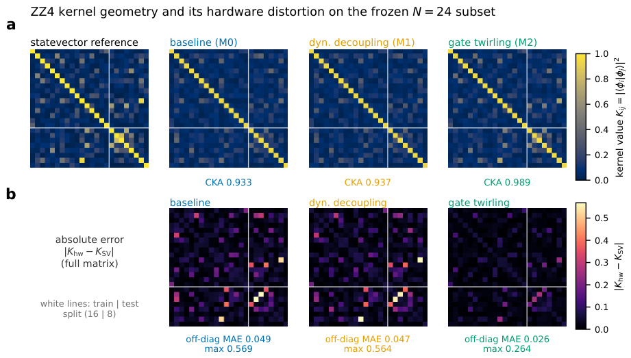
Figure 2.
Fixed-subset ZZ4 hardware-kernel geometry survival across three execution configurations. (a) Off-diagonal kernel entries (276 unordered pairs) of each hardware reconstruction against the statevector reference; points below the identity line show overlaps compressed toward a common background; the compression is strongest for baseline (M0) and weakest for gate twirling (M2). (b) Off-diagonal mean-squared error relative to the configuration-independent global finite-shot reference on the variance scale; the residual term dominates in every configuration (, conservative global reference). The split is a deterministic quadrature bookkeeping identity, not a physical noise-model decomposition (Section 2.12). (c) Centered geometric fidelity to the statevector kernel (full-matrix CKA) rises fromM0toM2; theM2improvement is window-resolved against bothM0andM1(, ; the diagonal-excluded contrasts are weaker, Supplementary Table S2.5), whereas theM1–M0contrast is unresolved (). (d) Absolute hardware label alignment (, point estimates; contrasts not window-resolved, ) falls as fidelity rises. The grey interval at right is the statevector-only label-permutation reference of Table 6 (null mean to , with the observed statevector and ); the revision-added per-regime references (Supplementary Table S2.6) place each hardware point at or below its own random-label mean (Section 3.3.3). Descriptive diagnostic on the frozen subset; single non-interleaved jobs onibm_fezat 1024 shots. No significance test or mitigation-efficacy claim is made.
Figure 2.
Fixed-subset ZZ4 hardware-kernel geometry survival across three execution configurations. (a) Off-diagonal kernel entries (276 unordered pairs) of each hardware reconstruction against the statevector reference; points below the identity line show overlaps compressed toward a common background; the compression is strongest for baseline (M0) and weakest for gate twirling (M2). (b) Off-diagonal mean-squared error relative to the configuration-independent global finite-shot reference on the variance scale; the residual term dominates in every configuration (, conservative global reference). The split is a deterministic quadrature bookkeeping identity, not a physical noise-model decomposition (Section 2.12). (c) Centered geometric fidelity to the statevector kernel (full-matrix CKA) rises fromM0toM2; theM2improvement is window-resolved against bothM0andM1(, ; the diagonal-excluded contrasts are weaker, Supplementary Table S2.5), whereas theM1–M0contrast is unresolved (). (d) Absolute hardware label alignment (, point estimates; contrasts not window-resolved, ) falls as fidelity rises. The grey interval at right is the statevector-only label-permutation reference of Table 6 (null mean to , with the observed statevector and ); the revision-added per-regime references (Supplementary Table S2.6) place each hardware point at or below its own random-label mean (Section 3.3.3). Descriptive diagnostic on the frozen subset; single non-interleaved jobs onibm_fezat 1024 shots. No significance test or mitigation-efficacy claim is made.
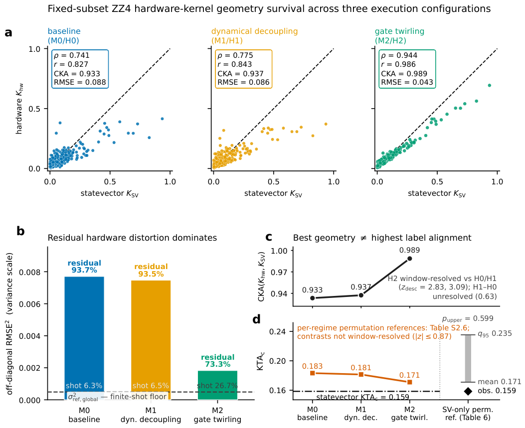
Figure 3.
Spectral flattening of the reconstructed ZZ4 hardware kernels. (a) Sorted eigenvalue spectra; the noiseless reference spectrum is peaked with a rapidly decaying tail, whereas the hardware tails are elevated, consistent with hardware-induced spectral flattening (Section 3.7). (b) Entropy effective rank per configuration against the statevector reference (); all hardware reconstructions are inflated, least under gate twirling ( vs /). Effective rank is computed from the uncentered spectrum. It is invariant to pure positive rescaling but not, in general, to the additive term, which the centered functionals (invariant under , ) annihilate, nor to non-affine changes in spectral shape. The simultaneously high CKA and inflated effective rank are therefore complementary rather than contradictory (Section 4.6). All hardware matrices retain the measured diagonal. Values are point estimates on the frozen subset, and the effective-rank ordering carries no window-level resolution.
Figure 3.
Spectral flattening of the reconstructed ZZ4 hardware kernels. (a) Sorted eigenvalue spectra; the noiseless reference spectrum is peaked with a rapidly decaying tail, whereas the hardware tails are elevated, consistent with hardware-induced spectral flattening (Section 3.7). (b) Entropy effective rank per configuration against the statevector reference (); all hardware reconstructions are inflated, least under gate twirling ( vs /). Effective rank is computed from the uncentered spectrum. It is invariant to pure positive rescaling but not, in general, to the additive term, which the centered functionals (invariant under , ) annihilate, nor to non-affine changes in spectral shape. The simultaneously high CKA and inflated effective rank are therefore complementary rather than contradictory (Section 4.6). All hardware matrices retain the measured diagonal. Values are point estimates on the frozen subset, and the effective-rank ordering carries no window-level resolution.
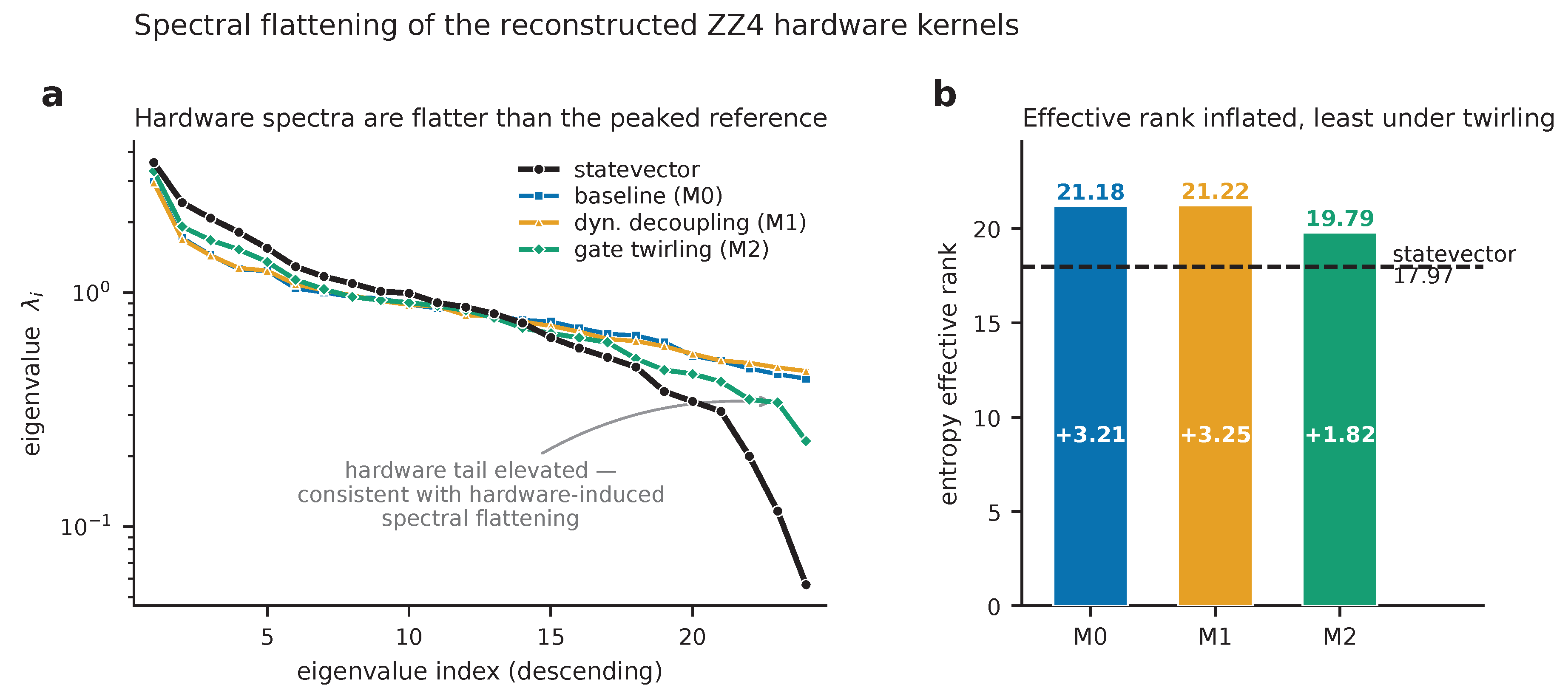
Disclaimer/Publisher’s Note: The statements, opinions and data contained in all publications are solely those of the individual author(s) and contributor(s) and not of MDPI and/or the editor(s). MDPI and/or the editor(s) disclaim responsibility for any injury to people or property resulting from any ideas, methods, instructions or products referred to in the content. |
© 2026 by the authors. Licensee MDPI, Basel, Switzerland. This article is an open access article distributed under the terms and conditions of the Creative Commons Attribution (CC BY) license (http://creativecommons.org/licenses/by/4.0/).
Copyright: This open access article is published under a Creative Commons CC BY 4.0 license, which permit the free download, distribution, and reuse, provided that the author and preprint are cited in any reuse.