
Submitted:
20 July 2026
Posted:
21 July 2026
You are already at the latest version
Abstract
Let ψ be the Chebyshev prime-counting function and π(x) the number of primes up to x. The Chebyshev-prime condition K(p)=li(ψ(p))−li(ψ(p−1))<1 is not equivalent to the sign rule ψ(p)−p>0. We prove that its leading threshold is the midpoint correction ψ(p)−p>12logp, with an explicit higher-order boundary, and define false Chebyshev primes through the resulting transition layer. Our main unconditional theorem shows that ordinary prime counting does not equidistribute logarithmic prime phases: for every nonzero integer combination τ of nontrivial zeta-zero ordinates, π(x)−1∑p≤xpiτ=xiτ/(1+iτ)+o(1). By contrast, the logarithmically uniform weight logp/p restores finite-dimensional Haar equidistribution for rationally independent ordinates. This dichotomy motivates the weighted local-time statistic L+(x)=2∑p≤x,p in the layer p−1/2. Under the Riemann hypothesis and linear independence, we conjecture the one-directional Cesàro law L+(x)/logx→fB(0), where fB(0) is the value at the origin of the limiting density of the symmetrized midpoint field B. Independently, we prove periodic and uniformly transverse quasiperiodic shrinking-target laws via coarea formulas. The remaining obstacles are tangential crossings of the zeta-derived field and transfer to the prime-sampled diagonal window.
Keywords:
Riemann hypothesis
; Chebyshev primes
; Chebyshev bias
; prime-phase equidistribution
; Weyl sums
; weighted local time
; occupation measure
; explicit formula
; transition layer
MSC: 11M26; 11N05; 11K36; 11N13; 11N37
1. Introduction
1.1. Chebyshev Primes and the -Adapted Prime Count
The Chebyshev functions and govern the primes through the explicit formula [1], and the Riemann hypothesis can be read from the size of the error: [2]. Robin [3] turned a divisor-sum growth estimate into a positivity criterion, and [4] observed that replacing x by the -adapted Riemann approximation recovers several further correct digits of . In that work the primes are probed one at a time, through the increment of across a prime,
directly analogous to Robin’s asymptotic study of [5], and a prime is a Chebyshev prime when . Since jumps by at p, is the li-measure of one prime jump, and says the jump is short: the local count momentarily lags the integers.
1.2. The Naive Sign Rule Fails by a Half-Jump
It is tempting and almost correct to identify with the sign rule . Section 2 shows this is wrong by a precise, deterministic amount: the correct threshold is not the endpoint excess but the midpoint excess , where is the midpoint of the jump interval. Equivalently the threshold moves from to . The primes obeying the naive rule but failing the true one, those with , are the false Chebyshev primes, and their counting function is the central object of the paper.
1.3. Why a Renormalized Field, and Why a Transition Layer
The half-jump correction is more than bookkeeping: it carries the same paired geometry as the analytic structure studied, on the zero side of the explicit formula, in the companion paper [6]. There the growth derivative of is organized by the paired kernel in the midpoint/half-separation coordinates , , and the sign structure of the associated field is governed by a thin transition layer in the pair variable a (bounded, in the conditional Riccati description, by ). The main result of [6] is in fact negative, the layer and the phase-aligned blocks it separates, cannot localize the positivity being sought, because the two paired sectors cancel to all algebraic orders, so we borrow from that paper only its geometry, the midpoint/half-separation splitting, and not any positivity mechanism. The Chebyshev test carries exactly this pair structure: a prime is examined through the pair , whose midpoint is and whose half-separation is : the same split. Passing to and removing the archimedean scale produces the renormalized Chebyshev field
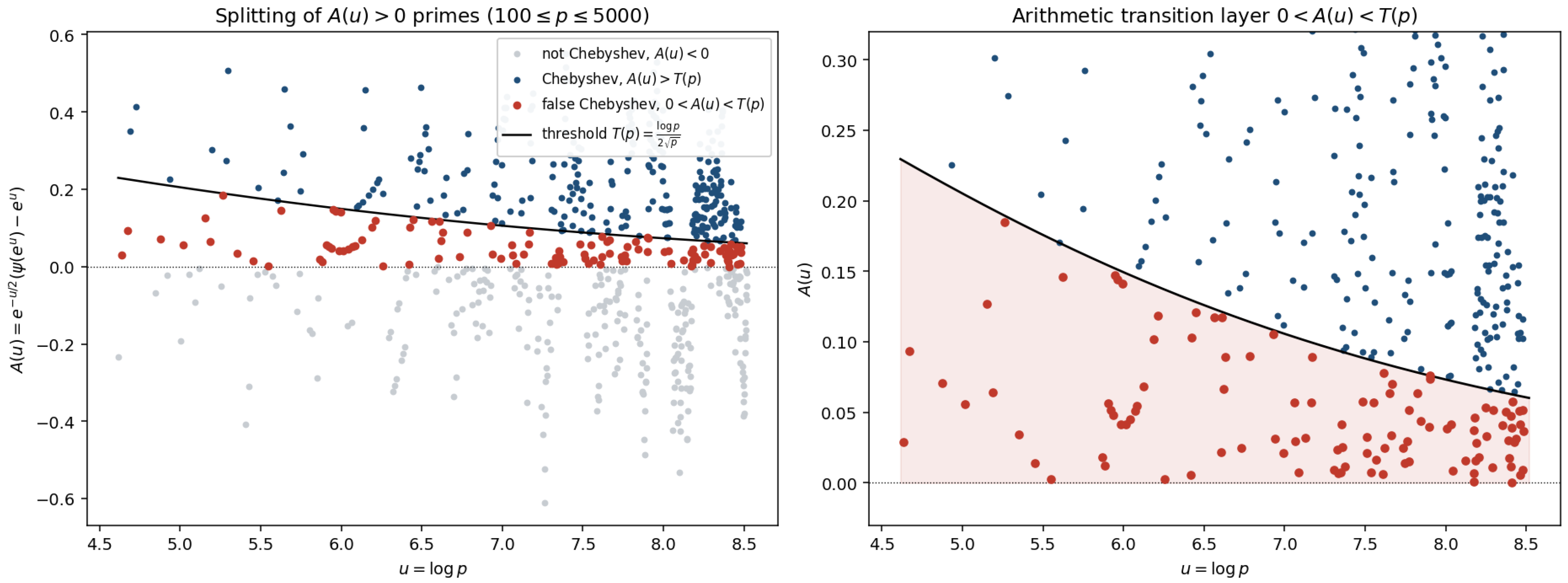
which plays, on the prime side, the role the theta kernel plays on the analytic side. In these terms the principal proxy layer for the false Chebyshev primes is about the zero level of A: a discrete, prime-sampled sign-transition layer in the same pair coordinates (the exact true set differs only by the boundary sliver of Proposition 3). This correspondence is the motivation for Definition 2; without it the false-positive set, and the field , would look arbitrary. Section 3 makes the dictionary explicit and Appendix A displays the splitting.
1.4. Results and Logical Status
We separate cleanly what is proved from what is conjectured, using the status convention: [A] fully proved (analytic), [C] conditional on a stated hypothesis, [N] high-precision numerical evidence on a specified range (not a computer-assisted proof). This convention is used consistently from here on.
Main results.
- A.
- Exact half-jump boundary [A] (Propositions 1–2): the Chebyshev-prime threshold is , not , with the exact correction located to within .
- B.
- Unweighted/weighted prime-phase dichotomy [A] (Theorems 1–2): ordinary prime counting does not equidistribute logarithmic phases of the zeta ordinates; the log-uniform weight restores Haar equidistribution.
- C.
- Weighted local-time formulation [C] (Conjecture 3): a one-directional Cesàro law under , replacing the withdrawn pointwise constant law; no converse to is claimed.
- D.
- Periodic and quasiperiodic shrinking-target theorems [A] (Theorems 7–8): the limiting occupation density of a shrinking window about a level set, identified by a coarea formula, unconditionally in the periodic case and under uniform transversality in the quasiperiodic case.
Items A, B, and D are unconditional ([A]) and constitute the paper’s proved core; item C is the paper’s central conditional contribution. B dictates which occupation statistic is meaningful (the weighted local time of C, not the raw count) and where the sole hard analytic step lies (the shrinking-window transfer named in D). D further isolates the remaining difficulty into two separate obstacles: a geometric tangency problem for the actual finite field, and the arithmetic prime-sampled diagonal transfer (Section 11).
The half-jump expansion and the exact boundary (Propositions 1–3) are [A]. The equidistribution obstruction (Theorem 1) and its log-uniform repair (Theorem 2) are [A]. These force a change of observable: the naive pointwise constant law is withdrawn. Corollary 1 shows, in a single-frequency continuum model, that the normalized count can remain logarithmically oscillatory, so the Rubinstein–Sarnak distribution alone does not justify a pointwise constant law for the actual prime count and is replaced by the weighted local-time law (Conjecture 3), a [C] statement conditional on and asserted in one direction only (Remark 6). The constant and the smoothness of the weighted statistic are [N] (Section 9). A coarser, -free secondary observable, the exponent of the unweighted count (Section 5), isolates the one RH-failing-regime step common to all such criteria. Section 7Section 8 place the criterion among those of Li, Robin, and Jensen. The weighted local-time law is one-directional and is not proposed as an equivalence; separately, the coarser exponent law (Section 5) is conjectured to be equivalent to , but neither direction of it is proved here.
2. Chebyshev Primes and the Half-Jump Correction
2.1. The Chebyshev-Prime Condition
Following [4], the local object is the increment of across a prime,
Since jumps by at p, the interval has length exactly .
Definition 1
(Chebyshev prime, [4]). A prime p is a Chebyshev prime if .
2.2. The Half-Jump Expansion (Proved)
Let , and let
Proposition 1
(Half-jump expansion). There is such that for all primes ,
In particular the leading correction to is : the Chebyshev threshold is the midpoint excess , not the endpoint excess . The precise curvature constant and the exact threshold are given in Proposition 2.
Proof.
Write . The single midpoint rule on the interval of half-width is exact up to
Here . Since we have , so the curvature term is ; we do not extract its constant here (the relative error is only because may differ from p by ), deferring the sharp value to Proposition 2. For the main term, with gives , whence
Adding the two contributions gives the displayed leading expansion; using produces the correction. □
The leading consequence of Proposition 1 is that the leading Chebyshev threshold is the midpoint excess , i.e. , not the endpoint excess .
Proposition 2
(Sharp boundary threshold). Write and
Then is continuous and strictly decreasing on its natural domain (where the lower limit of integration exceeds 1), since . As the lower endpoint , the integrand near and ; as , since the window has fixed length L while . By the intermediate value theorem therefore has a (unique, by monotonicity) root . Writing , the midpoint rule about gives with , so and the curvature term is . On the root scale ,
and solving therefore gives
Proof.
Monotonicity, continuity, and the two limits establishing existence are as displayed. The midpoint expansion and the value give the local form; setting the right side to 0 and solving the linear part gives the leading term . The remainder combines the contributions of both error terms in the local expansion, evaluated at : each of and is itself at that scale, and multiplying through by the reciprocal slope in solving for gives the stated . □
Remark 1.
This sharpens : the additive inside the numerator is a genuine correction (numerically, underestimates by 20– at ). We use Proposition 2 as the definition of the exact boundary.
2.3. The Exact Boundary and the False Chebyshev Primes
Proposition 3
(Exact sign boundary). For all sufficiently large primes p,
with the threshold of Proposition 2. Consequently the analytic proxy and the true set differ only on the sliver , of width .
Proof.
By Proposition 2, iff , where ; since is strictly decreasing this is the stated equivalence, and converts it to the threshold on . □
Definition 2
(True and proxy false-Chebyshev counts). A prime obeys the sign rule but not the Chebyshev condition when and . We distinguish the true count from its analytic proxy:
By Proposition 3 these differ only on the sliver of Proposition 2. All computations and conjectures below concern the proxy ; equality is verified up to (Section 9) but not proved for all large p.
Remark 2
(Why the proxy is empirically exact, [C/N]). By Proposition 3 a prime lies in the sliver only if falls within of . If one models the density of near that value as (Section 3), the expected number of sliver primes is, up to constants,
The prime sum converges (), giving an expected total of exceptions over all primes. This is a heuristic[C/N]estimate resting on the density model, not a proof; it is consistent with the observation that and agree with no exceptions up to (Section 9). Whether they agree for every large p is the one remaining boundary question (Problem a).
3. Motivation: A Paired-Coordinate Analogy from the Theta-Kernel Program
The companion theta-kernel study [6] recasts the growth derivative of , through the midpoint/half-separation coordinates , , as a paired-tail problem whose sign structure organizes around a thin transition layer in a. Its principal conclusion is a no-go theorem: that layer cannot be used to localize positivity of the growth derivative, since the two sectors of the decomposition cancel to all algebraic orders. What we transport to the prime side is therefore the pair-coordinate geometry alone, not any positivity mechanism. The Chebyshev-prime test carries the same pair structure: a prime is probed through , with midpoint and half-separation , playing the roles of a and b, and the zero level of the renormalized field below plays the role of the sign crossing of the companion paper’s transition layer.
Setting and renormalizing by gives the field . Under the explicit formula gives the almost-periodic representation [7]
and, since and with , Definition 2 becomes the shrinking-layer condition , the principal proxy layer for the false Chebyshev primes (the true set differing only by the boundary sliver of Proposition 3); we display this proxy layer in Appendix A.
It is cleaner to center the field at the midpoint of the explicit-formula jump. Writing for the symmetric normalization of , set
Then B places the false-positive threshold symmetrically about its own zero level, and B and A have the same almost-periodic part, hence the same limiting distribution and the same value of that density at the origin. We use B for the local-time law and keep A for the raw counting statements; the two differ only by the deterministic half-jump shift already isolated in Proposition 1.
4. The Equidistribution Obstruction and the Weighted Local-Time Law
The naive expectation is that for a constant C equal to the value at the origin of the limiting density of the field. We show that this pointwise law is not justified: the averaging measure implicit in it, in ordinary prime counting, is the wrong one for logarithmic phase. We then give the correct, log-uniform, averaging and the associated weighted local-time law.
4.1. Failure of Unweighted Logarithmic Equidistribution
Theorem 1
(Unweighted phase non-equidistribution). Let be real. Then
whose modulus is , bounded away from 0. In particular, for a nonzero integer combination of zeta ordinates, Weyl’s criterion fails and the logarithmic phases do not equidistribute on under ordinary prime counting.
Proof.
By the prime number theorem [8] in the form and partial summation,
the last step by integration by parts (the incomplete-gamma/ asymptotics). Dividing by gives the stated limit. Since is constant in x, the normalized sum does not tend to 0. □
Remark 3
(Endpoint concentration). The mechanism is that, in the coordinate , the primes concentrate near the right endpoint : the number in is , exponentially increasing in u. Ordinary counting is thus an exponentially weighted moving window of bounded logarithmic length near , not the long-interval average over that Weyl equidistribution requires. The Rubinstein–Sarnak limiting distribution [9], which lives in logarithmic () measure, therefore does not transfer directly to the cumulative count over .
Corollary 1
(No pointwise constant law). The heuristic is not supported by the Rubinstein–Sarnak distribution. Even in a single-frequency transversal model with the continuous prime density , the normalized count is asymptotically periodic in and has no limit; its logarithmic Cesàro mean equals . The numerical values at (Section 9) oscillate, consistent with this and not with monotone convergence.
The single-frequency computation behind Corollary 1 is elementary: near a zero of A the layer has logarithmic width , contributing primes; summing the geometric-like series over zeros spaced by gives , periodic in the offset to the nearest zero, with mean .
4.2. Log-Uniform Weighting Restores Equidistribution
The correct averaging weight is the one whose partial sums reproduce the flat -measure on . Since, by Mertens’ theorem, , the log-uniform weight is .
Theorem 2
(Weighted prime-phase equidistribution). Let be -linearly independent reals and . Then
Proof.
By the Weyl equidistribution criterion [10,11] and the Stone–Weierstrass theorem it suffices to treat characters , . For both sides equal 1 (using ). For , put (nonzero by linear independence), and set .
Write with (the prime number theorem). Then, by Riemann–Stieltjes partial summation,
Substituting , the main term t contributes
a bounded oscillatory expression (the log-free integral has no pole since ). The remainder contributes
Hence , and dividing by gives the claim for each fixed character. □
Remark 4
(On uniformity in the mode). The proof gives, for each fixed , that the k-th Fourier coefficient of the empirical measure tends to 0; by Weyl’s criterion this already yields equidistribution, since convergence of every fixed Fourier mode to the Haar value is exactly the criterion. No uniformity in k is needed for equidistribution itself. A quantitative discrepancy bound is a different matter and needs more than an effective prime number theorem: as the main term deteriorates and the error carries factors comparable to , while rational independence gives only with no lower bound on . A quantitative rate therefore requires an explicit Diophantine lower bound
together with uniform estimates for the twisted prime sums over the corresponding range of . We use only the qualitative theorem here and flag this Diophantine-plus-uniformity package as the input needed for the discrepancy rate in Level 2 of Section 11. Numerically the weighted sums stay uniformly small in τ (Section 9), consistent with this.
Remark 5.
Theorem 2 is the correct finite-dimensional foundation. The contrast with Theorem 1 is sharp: the same phases that fail to equidistribute under counting measure do equidistribute under the log-uniform measure , precisely because that measure undoes the endpoint concentration. Numerically (Section 9) the weighted Weyl sums decay at every tested τ, while the unweighted ones lock onto .
Corollary 2
(Fixed-window occupation). For -linearly independent and a window whose boundary has zero Haar measure,
where and is its pushforward (Rubinstein–Sarnak) distribution. If in addition 0 is a regular value of (so that, by the coarea formula, has a finite density continuous at 0), then
This is an iterated local-limit statement (fixed window, then , then ). Passing to the diagonal, prime-dependent, shrinking window remains the hard analytic step; but the underlying equidistribution is now on a correct footing.
4.3. The Weighted Local-Time Statistic
The layer has width in the units of the field. Dividing the log-uniform mass of each layer prime by that width,
which motivates the following occupation-time estimator.
Definition 3
(Weighted local time).
Conjecture 3
(Weighted local-time law). Under and , we conjecture that
where is the value at the origin of the limiting density of the symmetrized midpoint field B.
By Abel summation, and the unweighted count are related by the exact identity
The conjecture is therefore equivalent to only under the additional condition ; absent that, we retain the exact identity rather than an equivalence. Since is bounded in the accessible range, the boundary term contributes empirically, but we do not assume this.
Remark 6
(Status and honesty of the claim). Conjecture 3 is stated in one direction only: under we conjecture the weighted Cesàro limit. No reverse implication is established or presently expected; in particular, the weighted limit does not visibly encode , and we make no claim that implies . (We do not assert that such a reverse implication is impossible: a condition might imply without implying , only that none is available here.) This parallels the one-directional status of the growth criterion in [6]. The forward statement itself rests on the shrinking-window step of Corollary 2 (diagonal ), which is not supplied here and is the analytic heart of the problem.
The unweighted count remains available as a secondary observable, but only through its Cesàro mean: by Corollary 1, need not converge, whereas is a genuine ergodic average and is numerically far smoother (Section 9).
5. Secondary Programme: The Exponent Law
This section is a secondary programme, not used in the proof of any result in Section 4 or Section 11. The weighted local-time law of Section 4 is the paper’s primary occupation statistic and conditional contribution. We record here a second, coarser observable, the exponent of the unweighted count , which is weaker (it sees only the polynomial rate, not the constant) but has the advantage of being -free. It is included because it isolates, in the cleanest possible form, the single RH-failing-regime step that separates all of these criteria from a proof of ; nothing in this section is proved unconditionally, and no wording below should be read as suggesting the exponent law is proved or nearly proved. A reader interested only in the main dichotomy may skip directly to Section 6.
Let ; classically and , with .
Conjecture 4
(Exponent law). ; in particular the limit is if and only if holds.
Unlike the weighted local-time law, the exponent law reads the unweighted count, so it is not undermined by the equidistribution obstruction (Theorem 1): an obstruction to a pointwise constant is not an obstruction to a polynomial exponent. The exponent law splits into an upper bound (the exclusion step, which would yield ) and a lower bound. We record what is provable, what reduces to a clean model, and where the genuine obstruction lies. Throughout, is assumed (the interesting, RH-failing regime).
5.1. The Isolated Dominant-Profile Model
The trigonometric-profile model below is valid only under an explicit spectral hypothesis, which need not hold in general (the supremum may not be attained, there may be infinitely many zeros on , and there need be no gap below ).
Isolated dominant-profile hypothesis. Assume is attained by finitely many zeros, and that there exists with for every other nontrivial zero.
Under this hypothesis, set . The explicit formula splits the error into a dominant profile and a remainder,
where is almost-periodic. A false positive requires , i.e. forced within of 0. Absent the hypothesis this is a model not a reduction of the general RH-failing case.
5.2. A Model Theorem
Dropping the remainder isolates the geometry. Put and .
Theorem 5
(Model exponent bound, [A]). Let G arise from finitely many conjugate pairs, with only simple zeros and . Then for ,
Proof.
At a simple zero of G the profile crosses 0 with slope (transversality). Hence holds on a u-interval of width , i.e. an x-interval with . By the Brun–Titchmarsh inequality [12] the number of primes there is . Summing the geometric contribution over the crossings gives . □
The transversality hypothesis is the sublevel-set statement , valid for simple zeros with bounded below; tangential zeros give only , , and the bound weakens. The toy computation of Section 9 (, fitted exponents for ) is the numerical face of Theorem 5.
5.3. A Conditional Lower Bound for the Model Profile
The upper bound of Theorem 5 becomes essentially sharp once one assumes that the profile possesses sufficiently many transversal zero crossings.
Proposition 4
(Model lower bound, conditional). Suppose that the trigonometric profile
has only simple zeros and that there exist constants such that
and, strengthening the cumulative bound to a relative-density statement, every interval contains a zero with . (The cumulative bound alone does not guarantee a crossing near the terminal scale ; relative density does.) Assume further that the short-interval prime hypothesis
holds on the crossing intervals.
Then
for every .
Consequently,
Proof
(Proof sketch). By relative density there is a zero with ; we apply the crossing estimate below at , which is within of the terminal scale , so the resulting bound is a genuine estimate for rather than for a crossing that could be concentrated far below . Near a simple zero ,
Hence
holds on an interval of logarithmic width
Since the prime density in the variable is asymptotically
each crossing contributes
primes, provided the crossing interval, of length , contains the expected number of primes. For these intervals are shorter than , so this does not follow from the prime number theorem alone; we therefore add it as an explicit hypothesis,
which holds, for instance, under a suitable short-interval prime hypothesis, or in a continuum/prime-density model where is replaced by . Summing over the transversal crossings with gives
□
The upper bound of Theorem 5 uses only Brun–Titchmarsh and needs no analogue of ; it is therefore unconditional within the model.
5.4. The Obstruction for the True Error Term
For the genuine the remainder is not negligible here. Near a zero of D the condition reads , and since ranges up to the dominant profile is forced small only on the wider band , of u-width per crossing. The profile bound then yields only
which is only for , useless for . Recovering the sharp requires the density of at 0, under ordinary counting, to be and call this local-limit hypothesis . This is not the same statement as of Problem c: the latter is a log-uniform weighted statement at the fixed scale under , while is an ordinary-counting statement at a general RH-failing scale ; only their qualitative shape (a density estimate at a shrinking scale) is analogous. Thus the exclusion step does not reduce to a level-crossing estimate for the rightmost zeros alone: the critical-line fluctuation R must be controlled, and this requires , a hypothesis of the same general difficulty as, but logically distinct from, .
| Measure | log-uniform, | ordinary prime counting |
| Scale | fixed, | general, (RH-failing) |
| Regime | assumes | assumes fails |
| Used for | Conjecture 3 (§Section 4) | Prop. 5 (this section) |
| Status | Problem c, open | open, not reducible to Problem c |
5.5. Conditional RH Implication and the Lower Bound
Proposition 5
(Conditional exclusion, [C]). Assume the local-limit hypothesis for at scale near 0, under ordinary counting. Then , hence
The matching lower bound needs the profile to reach the layer with positive frequency: for a single dominant pair this is the transversal recurrence of a cosine, while several independent dominant frequencies require equidistribution on a torus (-type input). At the lower bound is exactly the occupation content of the weighted local-time law (Conjecture 3).
Remark 7.
The exponent is an occupation-time law: the frequency with which a recurrent almost-periodic field [13] visits an exponentially shrinking neighborhood of a level is set by the local geometry of its crossings, in the spirit of local-time/level-crossing theory and of the paired-tail sign geometry of [6].
6. GRH Version
For and a reduced class , set and . At a prime the jump of is , so the half-jump layer is , and
Let .
Conjecture 6
(GRH weighted local-time law). Let , so iff holds for modulus q. Define the progression-weighted local time
Then, under and for the zeros of , we conjecture
where is the value at the origin of the limiting density of the renormalized field .
The reduction mirrors Section 4 and Section 5 with the zeta zeros replaced by the zeros of the Dirichlet , and with the same correction: the unweighted count does not obey a pointwise law, for the same endpoint-concentration reason as Theorem 1, restricting to a progression does not restore unweighted equidistribution of logarithmic phase. The correct averaging is again the log-uniform weight on the progression, with normalizer , which produces the prefactor above. The exclusion step small is, as for , the hard direction, and is not claimed.
7. Logical Relations Among the Criteria
The status of the chain is as follows.
- Proposition 1 (half-jump expansion) and Proposition 3 (exact boundary) are [A].
- Theorem 1 (unweighted phases do not equidistribute) and Theorem 2 (log-uniform phases do) are [A].
- Conjecture 3 (weighted local-time law): under we conjecture , a logarithmic Cesàro statement.
- No reverse implication is established or expected (Remark 6); we claim no equivalence with .
Thus the weighted local-time criterion is one-directional: under we conjecture the weighted Cesàro limit, and the limit is not known to force . The exponent form is a distinct, weaker statement: the exponent law predicts under (Conjecture 4), but neither direction is proved, alone supplies no known lower occupation estimate for this exponentially thin prime-sampled layer. The reverse exclusion
would yield and is the one genuinely hard step (Proposition 5). We emphasize that we prove neither direction of the exponent law unconditionally; the interest of the exponent-law criterion is the exact identification of where the difficulty sits: in the shrinking diagonal window of Corollary 2, not a new route to .
8. Comparison with the Criteria of Li, Robin, and Jensen
It is useful to place the proposed criterion among established equivalents of .
Li’s criterion [14]: for all , where . It is an exact equivalence, spectral in nature (Weil’s explicit formula and positivity), with deep operator-theoretic content, but requires infinitely many coefficients.
Robin’s criterion [3]: positivity of an arithmetic prime-counting difference for all x (and, in its best-known form, for ). Exact, elementary to state, a global positivity statement over all x.
Jensen-polynomial hyperbolicity [15,16]: all Jensen polynomials of the -sequence are hyperbolic (real-rooted). Exact, geometric (real-rootedness/Turán inequalities), with the notable feature that hyperbolicity is unconditionally known for each fixed degree and all large shifts. In this last framework the difficulty concentrates in a thin finite strip of low shifts, where a recent analysis [17] shows that several independent local and inductive mechanisms (ratio barriers, frozen zero counts, interlacing lifts) fail simultaneously; a companion study [18] reads the same onset through a moment (Stieltjes) positivity structure attached to the -kernel. The present false-positive layer, the theta-kernel obstruction of [6], and these Jensen-side finite-strip phenomena share a recurring motif: an RH-equivalent problem in which the obstruction localizes to a thin critical region where every known local mechanism degenerates at once, though the regions and mechanisms differ from one setting to the next.
The proposed false-positive local-time criterion differs from all three in kind. It is not an exact finite or global positivity statement but an asymptotic law, and the observable is an occupation count: the frequency with which visits the half-jump layer, rather than the amplitude of any error term. This places it next to Chebyshev bias [19] and the Rubinstein–Sarnak limiting-distribution theory [9,20], and, heuristically, next to Brownian local time and level-crossing statistics. We make no claim that it is easier or more important than the classical criteria: the forward law is a demanding (but plausible) local limit theorem, and the reverse exclusion may be as hard as itself. Its interest is qualitative, it monitors a genuinely different statistic of the explicit-formula data, and it extends uniformly to , prime races, and Dirichlet L-functions (Section 6). We stress that is not itself a prime-race bias between residue classes (cf. Chebyshev bias [19]); it is a local-time bias of the Robin-regularized counting error, measuring recurrence of the normalized error to the half-jump layer, with the analytic pair geometry of Section 3 as its only link to the theta-kernel program, not a shared positivity mechanism, since [6] reaches a negative conclusion for that layer.
9. Numerical Results
Computations use a sieve of with by partial summation; is exact, and is evaluated by an 8-point Gauss–Legendre quadrature of , avoiding the cancellation of differencing li. We separate the evidence below by what each item tests: a proved theorem, a conjectural asymptotic, a finite-scale heuristic, or only internal numerical consistency, following the [A]/[C]/[N] convention throughout.
9.1. A. Exact/Proxy Boundary Verification ([N], Testing Proposition 3)
With this cancellation-free K, the criterion reproduces with no exceptions up to , consistent with the expected total of boundary exceptions (Remark 2); there are no false negatives. This tests the proved Proposition 3’s consequence that the proxy and true sets differ only on an explicitly bounded sliver — it is a finite-range check of an unconditional statement, not a test of any conjecture.
Up to there are 5028 false Chebyshev primes (5018 with ); up to , with . Table 1 reports , the ratio , and .
9.2. B. Unweighted Versus Weighted Weyl Sums ([N], Testing Theorems 1–2)
Table 2 exhibits Theorems 1 and 2 side by side. The unweighted normalized Weyl sum stays pinned at and does not decay, while the log-uniform weighted sum decays at every tested ordinate. Both theorems are unconditionally proved; this table is a finite-range numerical illustration of an already-proved dichotomy, not independent evidence for an open claim. It is the numerical heart of the paper.
9.3. C. Unweighted Count Versus Weighted Local-Time Statistic ([N], Bearing on Conjecture 3)
A log-log fit over gives slope , consistent with under (Conjecture 4, secondary programme). But does not stabilize, it reads and is non-monotone. This is consistent with the equidistribution obstruction (Theorem 1, Corollary 1): the data are nonmonotone and consistent with persistent oscillation. We claim no nonconvergence theorem for the full zeta field: Theorem 1 proves non-equidistribution of the phase vector, and the no-limit statement is established only for the single-frequency continuum model (Corollary 1). The weighted local-time statistic (Definition 3), by contrast, is markedly smoother: , and moves toward its conjectural limit , consistent with the behavior expected of a genuine ergodic average, though this range does not establish convergence. For the toy field (a finite-scale heuristic model, not a claim about the true zeta field), counting the same layer over gives fitted exponents for , in agreement with the predicted .
The constant ([N]).
The value at the origin of the limiting density of the symmetrized field, computed from the first ordinates with quadrature steps , is stable to the digits shown; the weighted statistic moves toward it slowly from below. We report this as evidence for , not as a certified limit of a counting statistic.
9.4. D. Window-Linearity Experiment ([N], Evidence for , Problem c)
Write , so . The shrinking-window statement predicts linear in c. Table 3 shows finite-range agreement with this at over a 32-fold range: tracks c to within . Thus the shape of , constant density across the shrinking layer, shows approximate linearity in the window width at ; this does not test the limit , the uniformity down to the diagonal window, the value , or the prime-transfer theorem, all of which remain open (Problem c). We have deliberately not established, and do not claim to have established, the diagonal shrinking-window limit itself.
9.5. E. Finite-Field Tangency Experiment ([N], Bearing on Theorem 8)
The two-frequency field is examined directly for the transversality hypothesis of Theorem 8: a coarea/Haar density computed by arcsine convolution (), a fixed-window time average (), and a grid search for points where vanishes on , locating genuine tangency candidates. Full detail and the numerical method are given at Remark 12 (Section 11); we do not repeat it here. This tests whether the actual finite zeta field satisfies the theorem’s hypothesis (it does not, unconditionally) and whether the theorem’s conclusion nonetheless holds in this finite computation (it is consistent with, but does not establish, an integrable tangency contribution).
9.6. F. Reproducibility
Every table and numerical claim in this section is regenerated by the accompanying reproducibility script from a clean environment; see the Data Availability Statement for the exact invocation, expected runtime, and a worked precision pitfall (float64 quadrature is insufficient for the Proposition 2 boundary check beyond –; the script uses arbitrary-precision arithmetic there instead).
10. Open Problems and Strategic Roadmap
The paper isolates five open problems. The first two are conceptually natural and plausibly tractable with current tools. The last three form the heart of the conditional local-time programme and of any possible exponent-law characterization of , and represent genuine hard problems whose resolution would require new analytic insights.
- label=(0)
- Exact eventual criterion. Show that for all sufficiently large p, ; equivalently, that no prime falls in the boundary sliver of Proposition 3. By Remark 2 the expected number of such primes is finite; the task is to make this a theorem (a Diophantine statement on near ).
- lbbel=(0)
-
Finite-zero / model exponent theorem.Prove, under uniform transversality and relative density of the zero crossings of the continuous profile (Theorem 8 and Section 11), together with a short-interval prime asymptotic on intervals of length , thatfor the finite-zero fieldwith -linearly independent and the corresponding model exponent. Note that this is not a statement about ordinary-counting equidistribution of , Theorem 1 shows that fails, but a statement about the density of primes in the crossing intervals of the continuous profile, which is a short-interval prime question, not an equidistribution question. The geometric half (transversality, crossing density) is addressed by Section 11; the arithmetic half is the short-interval hypothesis above. We regard this as the most promising near-term target.
- lcbel=(0)
-
Shrinking-window local limit (). Establish the quantitative log-uniform local statement of Section 4 under : with the log-uniform weight ,uniformly down to the diagonal window . Note sits at the very edge of the accessible range, which is exactly what makes this the hard step: Corollary 2 gives the statement for fixed (then , then ), and the open problem is to exchange the limits along the diagonal.This ingredient yields the weighted local-time law (Conjecture 3). It does not by itself yield the reverse exclusion, which is a separate RH-failing-regime statement (Problem d). Section 11 isolates the analytic geometry (Levels 1–2, unconditional) from this prime-distribution transfer (Level 3).
- ldbel=(0)
- Exclusion / reverse implication. Prove unconditionally that forces (Proposition 5); this is the step that would yield . Its core is not a level-crossing estimate for the rightmost zeros alone, that gives only (Section 5.4), but control of the density of at 0 at scale under ordinary counting, i.e. the hypothesis of Proposition 5, which is logically distinct from the weighted of Problem c.
- lebel=(0)
- GRH extension. Carry out (3)–(4) for Dirichlet L-functions (Conjecture 6), connecting with regularized Chebyshev-bias functions.
Why (3) and (4) are the true challenge.
Problems (3) and (4) are not artificial gaps. They are asking for a prime-sampled local limit theorem for
in shrinking windows of width , which is a much finer statement than the Rubinstein–Sarnak limiting distribution (which involves fixed windows and Lebesgue measure).
This is the place where any eventual RH equivalence would either be proved or fail. The difficulty lies at the intersection of:
- Almost-periodic functions and equidistribution;
- Shrinking-target problems on (not just tori);
- Prime-weighted sampling and self-correlation;
- Local-time asymptotics in number theory.
This problem is genuinely hard because the window width decreases as , the prime density is , and their product gives the delicate balance that makes plausible yet non-trivial. It is also the part that makes the paper scientifically interesting rather than merely a reformulation of RH.
11. Program: A Continuous Shrinking-Target Theorem and the Prime Transfer
The passage from fixed windows (Corollary 2) to the diagonal, prime-sampled, exponentially shrinking window separates naturally into three levels, a problem in the spirit of shrinking-target dynamics [21]. Level 1 treats periodic continuous fields; Level 2 treats quasiperiodic fields and the geometry of their zero hypersurfaces; Level 3 is the arithmetic transfer to logarithmically weighted prime samples. Levels 1–2 isolate the continuous geometric component, solved here in the periodic and uniformly transverse quasiperiodic cases; Level 3 remains conditional.
11.1. Level 1: A Continuous Shrinking-Target Local-Time Theorem (analytic)
The following is unconditional and elementary; it captures exactly the occupation geometry of a shrinking layer about the zero set of a periodic field.
Theorem 7
(Continuous shrinking-target local time). Let G be a , P-periodic function for which 0 is a regular value (all zeros simple), and set . Then
the right-hand side being the density at the origin of the pushforward of normalized Lebesgue measure on a period under G. (The integral starts at because makes the integrand undefined at the origin; this does not affect the limit.)
Proof.
Partition into full periods. Near a simple zero , , so the indicator set is an interval whose width is . Across such an interval is essentially constant: since and the interval has width , the relative variation is . Hence the set has length ; dividing by gives per crossing. Summing over the zeros in a period and over the periods, the error after division by U is , which tends to 0: the zeros have bounded density and , so by Cesàro averaging the mean of vanishes (indeed for the sum is bounded). The main term averages to . The identification of the right-hand side with the pushforward density at 0 is the coarea formula in one variable. □
Remark 8.
Numerically, for (zeros , ) the right-hand side is , and a direct evaluation at a resolvable fixed window returns ; for it returns , matching the single-frequency Cesàro mean of Corollary 1.
11.2. Level 2: Quasiperiodic Fields and the Coarea Target (Analytic)
Three distinct objects must be kept separate here: (i) the continuous quasiperiodic flow on ; (ii) the Haar/coarea zero-level density; and (iii) the weighted prime sampling of Theorem 2. Levels 1–2 concern (i)–(ii) only and involve no primes; the prime input enters at Level 3.
For a finite quasiperiodic field with -linearly independent, the Haar zero-level density is the coarea [22] (Kac–Rice [23,24]) integral
valid when 0 is a regular value. Since with , this equals the value at 0 of the N-fold convolution of the arcsine densities of the ; for two frequencies a direct evaluation gives , matching a torus histogram to three digits.
The continuous local-time theorem generalizes to the quasiperiodic setting under a transversality hypothesis.
Lemma 1
(Uniform zero-spacing under transversality). Under the hypotheses of Theorem 8 (in particular and ), the zeros of are simple and uniformly separated: there is , depending only on and (finite since on the compact torus), such that consecutive zeros of G are at distance . Consequently the zeros have bounded density ( per unit length), and there is (depending only on ) such that for every the η-crossing neighborhoods around distinct zeros are pairwise disjoint, uniformly in U.
Proof.
Since and is compact, and for all u. At a zero , ; by the mean value theorem , so keeps a fixed sign (hence G is strictly monotone) on , ruling out another zero in that interval. Thus consecutive zeros are separated by . Bounded density is immediate. For disjointness of -neighborhoods, note each has length (since near each simple zero once is small); taking with makes neighborhoods of consecutive zeros disjoint, and this threshold is independent of which zero or of U. □
Remark 9.
This lemma supplies exactly the facts Theorem 7’s proof uses informally (bounded zero density, so that ) and that Theorem 8’s proof uses in Step 3 (a U-independent threshold below which crossing neighborhoods are disjoint) and in Step 5 (the same bounded-density fact, transferred to the variable window). Crucially, depends only on , not on U, which is what licenses taking at fixed in Step 1 before letting in Step 4: no uniformity in η of the rate of convergence in U is needed, only this U-independent threshold.
Theorem 8
(Quasiperiodic shrinking-target local time). Let , let have rationally independent coordinates, and assume the flow is uniformly transverse to the zero hypersurface,
Put , and let satisfy and . Then
Remark 10.
The bound is stated globally for simplicity; the proof only uses it eventually (for u larger than some fixed ), since finitely many crossings below any fixed do not affect the Cesàro limit. The window is one-sided by design (only the upper half-jump layer is being modeled); near a simple zero this one-sided set has length regardless of the sign of (an upward crossing places the interval just after , a downward crossing just before it, but both have the same length), which is the constant appearing in the theorem. The two-sided window would instead have length , twice as large, since it covers both directions from , giving the coarser normalized limit in the periodic case; the paper consistently uses the one-sided convention throughout, matching the arithmetic half-jump layer .
Proof.
Fix a smooth even bump with and , and for set on ; this is smooth since .
Step 1 (unique ergodicity, fixed η). Since has rationally independent coordinates, the linear flow on is uniquely ergodic with respect to Haar measure [25,26]. As is continuous, unique ergodicity gives, for each fixed ,
Step 2 (coarea formula, ). Transversality forces 0 to be a regular value of F (if at then , contradicting the hypothesis), so the coarea formula applies and, by dominated convergence as approximates the Dirac mass at 0 along the fibers of F,
Step 3 (crossing sum vs. , uniform transversality). Write . Along , has , so at every zero of G; since , is bounded on compacta of the (compact) trajectory closure, so for small enough (depending only on and ) each zero is simple and isolated at scale , and on the interval of length around ,
Substituting (so ) and using ,
the error uniform over crossings by the uniform bound and the bound on F. Since is supported in , vanishes outside these crossing neighborhoods once is small enough that they are disjoint; summing over the crossings in (bounded density, by compactness of the trajectory and transversality) gives
so, dividing by U,
Step 4 (combine, then ). By Step 1 the left side tends to as for each fixed ; hence
and letting and invoking Step 2,
Step 5 (variable shrinking window). It remains to pass from the fixed crossing sum to the variable window . This is the local crossing calculation of Theorem 7: near each simple zero (now with uniformly, by transversality), the set has length since varies by a relative across the crossing interval (as ). Dividing by and summing as in the proof of Theorem 7 (the error terms again average to 0 by bounded crossing density and ) transfers the fixed-window limit of Step 4 to the variable-window statement of the theorem. □
Remark 11
(Flux measure versus coarea measure). A natural but mistaken shortcut is to argue directly that by unique ergodicity the crossing points equidistribute on , and then read off as the density of the crossing sum. This is not correct as stated: the crossings of the flow line with are distributed, as a point process on , according to the flux measure (with n the unit normal), not the ambient coarea measure itself, a standard fact from the theory of first-return (Poincaré) sections of flows. Weighting each crossing by , as the crossing sum in Theorem 8 does, is exactly what cancels this flux bias and recovers the coarea measure in the limit. The proof above sidesteps any need to reason about the flux measure directly: Steps 1–2 work entirely with the ambient Haar measure on via the mollifier , and the crossing-sum identity of Step 3 is derived from that route rather than assumed. The correct weight is thus a consequence of the argument, not an independent input, which is also why no other power of would give the stated limit.
Remark 12
(The transversality hypothesis is the real geometric issue, [N]). For the actual field the hypothesis to verify is on . This does not hold unconditionally: numerically, exhibits tangency points where vanishes on the zero set, so Theorem 8 does not apply directly to as stated. The mechanism of the failure is direct: Lemma 1’s zero-spacing bound degenerates as , so near a tangency zeros can cluster arbitrarily closely; the per-crossing weight in Theorem 8’s proof diverges there; and the U-independent threshold of Lemma 1, on which Step 3 of the proof of Theorem 8 depends, no longer exists globally. This tangency finding, and the fixed-window evaluation below, are numerical[N]claims: a direct time-average of the indicator at fixed over , compared against the arcsine-convolution coarea value, in double precision, with tangency points located by a grid search on . The conclusion of Theorem 8 is nonetheless observed to hold in this finite computation, against the coarea value , which is consistent with, but does not establish, an integrable tangency contribution; a proof must either establish a weaker transversality-in-measure condition or bound the tangential contribution directly. Thus tangencies, not qualitative equidistribution, are the remaining geometric obstacle at Level 2; controlling them is the strongest available next step short of the prime transfer.
11.3. Level 3: Transfer to Prime-Sampled Exponentially Shrinking Windows
The one genuinely conditional step is the transfer of Levels 1–2 from the continuous (or Haar) average to the prime-sampled average at the diagonal window . Concretely, one must upgrade Corollary 2 to
i.e. to exchange the limits and along the diagonal. This is where short-interval prime information enters: the window sits at the edge of the range accessible to the prime number theorem, so control here is of the same depth as short-interval prime distribution. We record this as the central open problem (Problem c).
Remark 13
(Summary of Section 11). Theorems 7 and 8 solve the continuous shrinking-target problem in the periodic and uniformly transverse quasiperiodic settings, identifying the limit by a coarea formula. For the finite zeta field , tangential crossings remain a geometric issue (Remark 12); this is a theorem under uniform transversality, not an unconditional statement about itself. After that issue is controlled, the remaining step is the arithmetic transfer to the prime-dependent diagonal window of Level 3, a separate obstacle governed by short-interval prime distribution.
12. Conclusions and Outlook
This paper rests on three unconditional pillars. The first is the exact half-jump boundary (Propositions 1–2): the Chebyshev-prime condition is governed not by the sign of but by its midpoint-corrected threshold , with the exact correction located precisely. The second is the prime-phase equidistribution dichotomy (Theorems 1 and 2): logarithmic phases of the zeta ordinates fail to equidistribute under ordinary prime counting, yet equidistribute exactly under the log-uniform weight . The third is the periodic and uniformly transverse quasiperiodic shrinking-target local-time theorem (Theorems 7 and 8), which identifies the limiting occupation density of a shrinking window about a level set by a coarea formula, independently of any arithmetic input.
The conceptual lesson uniting the first two pillars is that ordinary prime counting is the wrong averaging measure in logarithmic phase: primes below x concentrate near in the coordinate , so counting measure behaves like a bounded-length moving window rather than a long-interval average, and Weyl’s criterion fails as a result. The weight restores exactly the flat -measure that equidistribution requires, and every downstream observable, the local-time statistic, the fixed-window occupation, the finite-dimensional equidistribution theorem, is built on this corrected measure rather than on counting measure.
This dictates the paper’s conditional programme. The weighted local-time law (Conjecture 3) is conjectured under and linear independence of the ordinates, and is stated in one direction only: we do not assert, and see no route to, a converse implication to , still less an equivalence. A single asymptotic constant cannot encode the linear independence of infinitely many ordinates, and the forward direction itself rests on an unproved shrinking-window transfer (Problem c).
Two distinct obstacles remain, and it is important that they not be conflated. The first is geometric: Theorem 8 solves the quasiperiodic shrinking-target problem under uniform transversality , but the actual finite field exhibits tangential crossings where this hypothesis fails (Remark 12); resolving this requires either a transversality-in-measure argument or a direct bound on the tangential contribution, and is independent of any arithmetic difficulty. The second is arithmetic: even granting the geometric problem, the transfer from fixed or Haar windows to the prime-sampled diagonal window (Level 3, Problem c) sits at the edge of what the prime number theorem controls and is of the same depth as short-interval prime distribution. Neither obstacle reduces to the other.
The exponent-law programme of Section 5 is deliberately kept separate from this main line. It is a coarser, -free observable, valid only under the isolated dominant-profile hypothesis in the RH-failing regime, and we prove neither direction of it unconditionally: the exponent law predicts under , but alone supplies no known lower occupation estimate for this exponentially thin layer, and the reverse exclusion requires the same order of local-density control as the main programme.
On the numerical side, we have tested: the half-jump proxy against the true Chebyshev set up to (no exceptions found); the equidistribution dichotomy via unweighted and weighted Weyl sums at several zeta ordinates; the weighted local-time statistic against the unweighted count across ; window linearity at the single scale ; and the periodic and two-frequency quasiperiodic shrinking-target identities, including a direct tangency search for . We have not tested, and do not claim to have tested, the diagonal shrinking-window limit itself, its uniformity in x, or any instance of the exponent law.
Several directions follow naturally. The tangency structure of invites a direct study of , most tractably in the two- and three-frequency cases where the zero set is an explicit curve on the torus. The short-interval hypothesis underlying Proposition 4 and the diagonal transfer of Level 3 both call for quantitative short-interval prime estimates sharper than what is unconditionally known. The analogue of Section 6 is structurally parallel and would benefit from the same treatment once the case is further advanced. Finally, the quasiperiodic shrinking-target theorem (Theorem 8) is of independent interest in dynamics and is not tied to the arithmetic application here; it applies to any uniformly transverse quasiperiodic flow and target function.
None of this reduces to a routine remaining step. The dichotomy and the shrinking-target theorems are unconditional and load-bearing, but the passage from them to any statement about , in either the weighted or the exponent-law form, requires genuinely new input at exactly the two points identified above.
Funding
This research received no external funding.
Data Availability Statement
The reproducibility supplement accompanying this paper, a Python script, a data file with the first 1000 nontrivial zeta ordinates, a README, and CSV outputs for every table and numerical claim in the paper, is provided alongside the manuscript and has been executed from a clean environment in both a quick () and full (, matching the tables in the paper) configuration. The boundary check at (Section 3) uses the same script in an opt-in slower mode; see the supplement’s README for exact invocation and expected runtime.
Acknowledgments
The author acknowledges the use of generative AI tools, including OpenAI’s ChatGPT 5.5 and Anthropic’s Claude Opus 4.8, for assistance with numerical checks, consistency verification, language refinement, and editorial suggestions during the preparation of this manuscript. All mathematical results, proofs, interpretations, and conclusions were independently reviewed and validated by the author, who assumes full responsibility for the content of the paper.
Conflicts of Interest
The author declares no conflicts of interest.
Appendix A. The False Chebyshev Primes
Figure A1 shows, for , the splitting of the primes by : among primes with , those above the threshold are genuine Chebyshev primes (blue), those in the proxy layer are (proxy) false Chebyshev primes (red); (gray) are non-Chebyshev. (The exact true set differs from the proxy layer only by the boundary sliver of Proposition 3, of width , invisible at this resolution.)
Figure A1.
Splitting of the primes into genuine Chebyshev primes (, blue) and proxy false Chebyshev primes (, red), for . The red points are the arithmetic proxy transition layer; the black curve is the half-jump threshold .
Figure A1.
Splitting of the primes into genuine Chebyshev primes (, blue) and proxy false Chebyshev primes (, red), for . The red points are the arithmetic proxy transition layer; the black curve is the half-jump threshold .
Counts.
, , , (of which 5018 have ).
Small primes.
The ten false Chebyshev primes with are .
First false Chebyshev primes with p>100.
References
- H. Davenport, Multiplicative Number Theory, 3rd ed., revised by H. L. Montgomery, Graduate Texts in Mathematics 74, Springer, 2000.
- Titchmarsh, E. C. The Theory of the Riemann Zeta-Function, 2nd ed.; Heath-Brown, D. R., Ed.; Oxford University Press, 1986. [Google Scholar]
- Robin, G. Grandes valeurs de la fonction somme des diviseurs et hypothèse de Riemann. J. Math. Pures Appl. 1984, 63(9), 187–213. [Google Scholar]
- Planat, M.; Solé, P. Efficient prime counting and the Chebyshev primes. J. Discrete Math. Article ID 491627, 11 pp. 2013. [Google Scholar]
- Robin, G. Sur la différence Li(θ(x))-π(x). Ann. Fac. Sci. Toulouse Math. 1984, 6, 257–268. [Google Scholar] [CrossRef]
- Planat, M. Nonlocal cancellation in a theta-kernel decomposition of the Riemann Ξ-growth derivative: an obstruction to phase-aligned blockwise positivity. Mathematics in review. 2026. [Google Scholar] [CrossRef]
- Jessen, B.; Wintner, A. Distribution functions and the Riemann zeta function. Trans. Amer. Math. Soc. 1935, 38, 48–88. [Google Scholar] [CrossRef]
- Ingham, A.E. The Distribution of Prime Numbers. In Cambridge Tracts in Mathematics and Mathematical Physics; Cambridge University Press, 1932; Volume No. 30. [Google Scholar]
- Rubinstein, M.; Sarnak, P. Chebyshev’s bias. Exp. Math. 1994, 3, 173–197. [Google Scholar] [CrossRef]
- Weyl, H. Über die Gleichverteilung von Zahlen mod. Eins Math. Ann. 1916, 77, 313–352. [Google Scholar] [CrossRef]
- Kuipers, L.; Niederreiter, H. Uniform Distribution of Sequences. In Pure and Applied Mathematics; Wiley-Interscience, 1974. [Google Scholar]
- Montgomery, H. L.; Vaughan, R. C. Multiplicative Number Theory I: Classical Theory. In Cambridge Studies in Advanced Mathematics; Cambridge University Press, 2007; Volume 97. [Google Scholar]
- Besicovitch, A. S. Almost Periodic Functions; Cambridge University Press, 1932. [Google Scholar]
- Li, X.-J. The positivity of a sequence of numbers and the Riemann hypothesis. J. Number Theory 1997, 65, 325–333. [Google Scholar] [CrossRef]
- Csordas, G.; Norfolk, T. S.; Varga, R. S. The Riemann hypothesis and the Turán inequalities. Trans. Amer. Math. Soc. 1986, 296, 521–541. [Google Scholar] [CrossRef]
- Griffin, M.; Ono, K.; Rolen, L.; Zagier, D. Jensen polynomials for the Riemann zeta function and other sequences. Proc. Natl. Acad. Sci. USA 2019, 116, 11103–11110. [Google Scholar] [CrossRef] [PubMed]
- Planat, M. Asymptotic hyperbolicity of Jensen polynomials and the finite-strip obstruction to the Riemann hypothesis. Mathematics 2026, 14(no. 11), 1884. [Google Scholar] [CrossRef]
- Planat, M. Parity bifurcation, PIII(D6) topology, and a Stieltjes framework to Jensen polynomial hyperbolicity. Mathematics 2026, 14(no. 13), 2240. [Google Scholar] [CrossRef]
- Almadhi, A.; Planat, M.; Solé, P. Chebyshev’s bias and generalized Riemann hypothesis. arXiv 2011, arXiv:1112.2398. [Google Scholar]
- Akbary, A.; Ng, N.; Shahabi, M. Limiting distributions of the classical error terms of prime number theory. Quart. J. Math. 2014, 65, 743–780. [Google Scholar] [CrossRef]
- Hill, R.; Velani, S. L. The ergodic theory of shrinking targets. Invent. Math. 1995, 119, 175–198. [Google Scholar] [CrossRef]
- Federer, H. Geometric Measure Theory; Springer, 1969. [Google Scholar]
- Adler, R. J.; Taylor, J. E. Random Fields and Geometry; Springer, 2007. [Google Scholar]
- Cramér, H.; Leadbetter, M. R. Stationary and Related Stochastic Processes: Sample Function Properties and Their Applications; Wiley, 1967. [Google Scholar]
- Katok, A.; Hasselblatt, B. Introduction to the Modern Theory of Dynamical Systems; Cambridge University Press, 1995. [Google Scholar]
- Walters, P. An Introduction to Ergodic Theory. In Graduate Texts in Mathematics; Springer, 1982; Volume 79. [Google Scholar]

Table 1.
False Chebyshev prime counts and exponent estimates (all primes).
| x | |||
|---|---|---|---|
| 186 | |||
| 605 | |||
| 1789 | |||
| 5028 |
Table 2.
Unweighted prime-phase sums stay near (non-equidistribution, Theorem 1); log-uniform weighted sums decay (equidistribution, Theorem 2).
Table 2.
Unweighted prime-phase sums stay near (non-equidistribution, Theorem 1); log-uniform weighted sums decay (equidistribution, Theorem 2).
| x | unweighted | weighted | ||
|---|---|---|---|---|
Table 3.
Linearity of the layer occupation in the window width at : numerical evidence for approximate linearity in the window width. This tests linearity in c at one finite x, not the limit or the diagonal transfer ().
Table 3.
Linearity of the layer occupation in the window width at : numerical evidence for approximate linearity in the window width. This tests linearity in c at one finite x, not the limit or the diagonal transfer ().
| c | |||
|---|---|---|---|
| 1241 | |||
| 2487 | |||
| 1 | 5028 | ||
| 2 | 10203 | ||
| 4 | 20407 | ||
| 8 | 40261 |
Disclaimer/Publisher’s Note: The statements, opinions and data contained in all publications are solely those of the individual author(s) and contributor(s) and not of MDPI and/or the editor(s). MDPI and/or the editor(s) disclaim responsibility for any injury to people or property resulting from any ideas, methods, instructions or products referred to in the content. |
© 2026 by the authors. Licensee MDPI, Basel, Switzerland. This article is an open access article distributed under the terms and conditions of the Creative Commons Attribution (CC BY) license (http://creativecommons.org/licenses/by/4.0/).
Copyright: This open access article is published under a Creative Commons CC BY 4.0 license, which permit the free download, distribution, and reuse, provided that the author and preprint are cited in any reuse.


