

Submitted:
20 July 2026
Posted:
21 July 2026
You are already at the latest version
Abstract
Feature selection remains a fundamental challenge in modern machine learning, particularly in ultra-high-dimensional domains such as genomics, text mining, cybersecurity, and bioinformatics, where the number of features can exceed the number of samples by several orders of magnitude. Traditional filter, wrapper, and embedded feature selection methods often require evaluating every feature directly, incurring substantial computational costs and limiting scalability. In this paper, we propose Label-Aware Sketch-Based Feature Selection (LSFS), a novel supervised feature selection framework that reformulates feature selection as a similarity retrieval problem in compressed sketch space. LSFS constructs MinHash or weighted MinHash signatures for feature columns and the label vector, applies locality-sensitive hashing (LSH) to retrieve a small subset of potentially relevant features, and performs exact statistical refinement and redundancy elimination only on the retrieved candidates. This strategy substantially reduces the number of features requiring expensive evaluation while preserving predictive information relevant to the target labels. The proposed framework is evaluated on ten high-dimensional benchmark datasets spanning gene expression analysis, toxicology, sparse classification, image-derived feature spaces, and mass-spectrometry applications. Experimental results demonstrate that LSFS achieves predictive performance competitive with established filter, wrapper, embedded, and nonlinear feature selection methods across LR, RF, and Support Vector Machine classifiers. At the same time, LSFS reduces the average feature search space from 17,234 original features to approximately 1,176 retrieved candidates, corresponding to an average reduction of 85.54\% before exact refinement. On the largest datasets, the reduction exceeds 97\% while maintaining competitive classification performance. These results demonstrate that sketch-based retrieval can serve as an effective and scalable preprocessing mechanism for supervised feature selection. The proposed framework introduces a new feature-centric use of MinHash and locality-sensitive hashing, providing a practical approach to feature selection in ultra-high-dimensional learning problems.
Keywords:
feature selection
; locality-sensitive hashing (LSH)
; MinHash
; high-dimensional data
; machine learning
; dimensionality reduction
; similarity search
; scalable learning algorithms
1. Introduction
High-dimensional data have become increasingly common across a wide range of scientific and industrial applications, including genomics, bioinformatics, text mining, cybersecurity, recommender systems, healthcare analytics, and image processing. In many of these domains, datasets contain tens of thousands or even millions of features while only a limited number of samples are available, resulting in the well-known “” setting. Although such datasets contain rich information, the presence of large numbers of irrelevant, redundant, and noisy features often degrades predictive performance, increases computational requirements, and reduces model interpretability. Consequently, feature selection has become a fundamental component of modern machine learning pipelines.
Feature selection aims to identify a subset of informative features while preserving or improving predictive performance. Existing methods are commonly categorized into filter, wrapper, and embedded approaches. Filter methods evaluate features using statistical criteria such as correlation, mutual information, chi-square statistics, or information gain. Wrapper methods search for feature subsets based on the performance of a predictive model, while embedded methods integrate feature selection directly into the learning process through regularization or model-specific mechanisms. Representative examples include minimum Redundancy Maximum Relevance (mRMR), Relief-based methods, LASSO, HSIC-Lasso, decision-tree-based approaches, and numerous hybrid variants. Despite their success, most existing methods require repeated evaluation of large numbers of features, feature pairs, or feature subsets, leading to computational and memory requirements that grow rapidly with dimensionality. The challenge becomes particularly severe in ultra-high-dimensional settings such as genomic analysis, text mining, and sparse representation learning, where the number of features may exceed hundreds of thousands or millions. Even scalable implementations of classical feature selection algorithms remain fundamentally tied to the original feature space and often require repeated scans of the data matrix, pairwise similarity calculations, or optimization procedures. As a result, there is a growing need for approximate, scalable feature selection frameworks that identify relevant and redundant features without directly operating on the full high-dimensional representation.
In parallel, sketching and hashing techniques have emerged as powerful tools for scalable similarity estimation and large-scale data processing. Among these approaches, MinHash and Locality-Sensitive Hashing (LSH) have become widely used for approximate nearest-neighbor search, near-duplicate detection, large-scale retrieval, and similarity estimation in domains ranging from web search to genomics. The central idea behind these methods is to compress high-dimensional objects into compact signatures while preserving similarity relationships with high probability. This enables efficient processing of massive datasets using representations that are substantially smaller than the original data. Despite their success, existing applications of MinHash and LSH have focused almost exclusively on instance-level representations, where rows or objects are hashed to support retrieval, clustering, indexing, or similarity search. Comparatively little attention has been devoted to exploiting these techniques directly for supervised feature selection. Furthermore, most existing feature selection methods continue to operate in the original feature space, relying on statistical, optimization-based, or model-based relevance measures rather than similarity-preserving sketches. This observation reveals an important research gap: if compact hash signatures can effectively preserve similarity relationships among high-dimensional objects, can they also be used to estimate feature relevance and redundancy in a scalable feature-selection framework?
To address this question, we introduce a novel Label-Aware Feature Selection framework based on MinHash and Locality-Sensitive Hashing, which we refer to as LSFS. Unlike traditional applications of MinHash that operate on samples, our approach treats feature columns as the primary objects to be hashed. We further construct signature representations for both features and class labels, enabling feature relevance estimation directly within the compressed signature space. By interpreting signature collisions and Jaccard-style similarities as surrogates for feature–label association and feature redundancy, the proposed framework transforms supervised feature selection into a similarity-search problem. Locality-Sensitive Hashing is then employed to efficiently identify candidate relevant and redundant features without requiring exhaustive pairwise comparisons. The primary contributions of this work are summarized as follows:
- We propose a novel feature-centric MinHash framework that constructs compact signature representations for both feature columns and class labels, enabling supervised feature selection in compressed sketch space.
- We introduce a label-aware relevance estimation mechanism based on MinHash collisions and Jaccard-style similarities, providing an efficient approximation of feature–label association.
- We develop an LSH-based candidate-generation strategy that identifies potentially relevant and redundant features without exhaustive pairwise comparisons.
- We present a scalable feature selection pipeline suitable for ultra-high-dimensional datasets arising in domains such as genomics, text mining, and other large-scale machine learning applications.
- We empirically evaluate the proposed framework on benchmark and high-dimensional datasets and demonstrate its effectiveness as a scalable alternative to traditional feature selection approaches.
The remainder of this paper is organized as follows. Section 2 reviews the theoretical foundations of feature selection, MinHash, weighted MinHash, and Locality-Sensitive Hashing. Section 3 discusses related work in hashing-based learning and scalable feature selection. Section 4 presents the proposed LSFS framework. Section 5 describes the experimental setup and evaluation methodology, while Section 6 presents and discusses the results. Finally, Section 7 concludes the paper and outlines future research directions.
2. Background
2.1. Feature Selection in High Dimensions
In supervised learning, feature selection seeks a subset such that a predictor trained on achieves maximal generalization performance. Filter methods estimate relevance independent of any model, most commonly via correlation, mutual information, or statistical tests. Wrapper and embedded methods optimize subsets using predictive models. Classical embedded approaches include the Least Absolute Shrinkage and Selection Operator (LASSO) [1,2], which performs feature selection through sparsity-inducing regularization. However, in ultra-high dimensions, even filter methods become computationally expensive since they require evaluation of relevance for every feature.
2.2. MinHash and Jaccard Similarity
For two sets A and B, Jaccard similarity is defined as
MinHash constructs a randomized estimator of such that
where is a randomized hash function induced by a random permutation. Repeating this process k times yields a signature vector whose collision frequency estimates the Jaccard similarity.
2.3. Weighted MinHash
For non-binary, non-negative vectors , generalized Jaccard similarity is defined as
Consistent weighted sampling (CWS) generates hash signatures whose collision probability equals , extending MinHash to continuous-valued features.
2.4. Locality-Sensitive Hashing
Locality-sensitive hashing defines a family of hash functions such that similar objects collide with high probability while dissimilar objects do not. Using banding, a signature matrix is divided into b bands of r rows. Two objects become a candidate pair if they match in any band. The candidate probability follows
where s is the similarity.
3. Related Work
Our work lies at the intersection of three streams of research: (i) locality-sensitive hashing (LSH) and MinHash for scalable similarity search, (ii) hashing-based dimensionality reduction and representation learning, and (iii) instance/feature selection for high-dimensional and big-data settings, including genomics and text.
3.1. Locality-Sensitive Hashing and MinHash Foundations
Locality-sensitive hashing was originally proposed to support efficient approximate similarity search in high-dimensional spaces by designing hash functions whose collision probabilities reflect the similarity between objects [3,4]. The classical theoretical framework of LSH focuses on designing families of hash functions that are sensitive to specific distance measures (e.g., Jaccard, cosine, or distances) and provides probabilistic guarantees on query-time and space usage [3,4]. In this context, MinHash is a well-known scheme for approximating Jaccard similarity, especially on sparse binary sets or bag-of-words representations. It underpins many near-duplicate detection and large-scale retrieval systems.
Andoni and Indyk later refined LSH for angular distances and provided practical and provably optimal schemes [4]. Recent work has also explored the use of locality-sensitive hashing to handle high-dimensional data by projecting it into lower-dimensional spaces. PM-LSH introduces an efficient LSH-based framework for approximate nearest-neighbor search that projects high-dimensional data into a lower-dimensional space using locality-sensitive hash functions and then performs indexing and retrieval in the projected domain [5]. The framework combines projection-based dimensionality reduction with efficient distance estimation and indexing structures, demonstrating that LSH can be an effective tool for preserving similarity relationships while reducing the computational burden of processing high-dimensional data. However, these approaches focus primarily on similarity search and approximate nearest-neighbor retrieval rather than supervised feature relevance estimation or feature subset selection.
3.2. Hashing-Based Representation Learning and Dimensionality Reduction
A parallel line of work uses hashing to construct compact binary representations of high-dimensional data, mostly for retrieval but also implicitly for dimensionality reduction. Spectral Hashing learns data-dependent binary codes by approximating the eigenvectors of a graph Laplacian, matching the distribution of data under certain assumptions and preserving neighborhood relationships [6]. Semantic Hashing learns binary codes using deep autoencoder-style architectures so that similar documents are mapped to nearby codes in Hamming space; it has been shown to outperform LSH for document retrieval in many cases [7]. Linear Spectral Hashing further simplifies spectral hashing by using linear approximations to the Laplacian eigenvectors, making hashing more scalable to larger datasets [8].
From a broader dimensionality-reduction perspective, Ray et al. provide a comprehensive review of techniques for high-dimensional data analysis, including feature extraction (e.g., PCA, manifold learning) and feature selection methods [9]. While hashing-based methods are primarily described as tools for similarity search and efficient indexing, they are not framed as supervised feature-selection mechanisms operating directly on the feature dimension. Our proposal differs in that it explicitly treats MinHash/LSH over feature indices as a first-class mechanism for dimension reduction and feature relevance estimation.
In the big-data setting, Ramírez-Gallego et al. propose an information-theoretic feature selection framework on Apache Spark, implementing a range of filter-type feature selection methods (e.g., mutual information and related criteria) in a distributed fashion [10]. Their focus is on scalability of classical filter methods; hashing does not play a central role beyond potential implementation optimizations.
3.3. LSH for Instance and Feature Selection
Recent studies have explored the use of hashing within feature selection frameworks. For example, UAFS-BH [11] learns binary hash codes that serve as weak supervision signals to guide unsupervised feature selection. However, the hashing mechanism is primarily used to generate surrogate labels, while feature importance is determined through a subsequent optimization framework. In contrast, LSFS directly exploits MinHash and locality-sensitive hashing to estimate feature-label relevance and perform feature ranking without requiring graph construction, pseudo-label generation, or iterative optimization. These approaches remain instance-centric and treat feature selection as a separate, largely classical statistical step, rather than leveraging hash collisions or signatures to define feature–feature similarity.
Recent research has continued to improve the efficiency and effectiveness of locality-sensitive hashing through advanced indexing and bucket management strategies. DB-LSH [12] introduces a query-based dynamic bucketing mechanism that reduces boundary effects and improves candidate quality while maintaining theoretical guarantees for approximate nearest-neighbor retrieval. More recently, DET-LSH and its parallel extension PDET-LSH [13] proposed a dynamic encoding tree structure to accelerate index construction and range-query processing in high-dimensional spaces, achieving substantial improvements in indexing and query efficiency while preserving the probabilistic guarantees of traditional LSH frameworks. These methods demonstrate the continued evolution of LSH for scalable similarity search; however, their primary objective remains efficient retrieval rather than supervised feature selection.
Dagdia and coauthors introduced rough-set-based methods that are much closer to hash-based data compression. In [14], they propose a scalable rough set theory (RST) based approach for big-data preprocessing that uses distributed computation to approximate discernibility relations and reducts. In a follow-up work, they introduce LSH-dRST, which uses LSH to approximate the RST-based discernibility matrix, thereby reducing computational cost while preserving decision-quality properties [15]. Although LSH-dRST does exploit hashing for feature selection, the focus is on rough set reduct computation; signatures are applied to instances (objects) and the logic of reduction is governed by RST. Our work instead builds MinHash signatures directly at the level of feature columns and uses Jaccard-style similarities between feature signatures, thereby framing the feature-selection problem as a scalable, approximate correlation- or redundancy-filtering task.
Beyond these rough-set and review-based contributions, several works explore instance and variable selection strategies in big data without directly using MinHash. Settouti et al. propose a joint instance and variable selection approach for pixel-based remote sensing classification, emphasizing cost reduction during learning while maintaining classification performance [16]. Tsamardinos et al. study greedy feature selection algorithms tailored to high-dimensional big data, with a strong emphasis on statistical reliability and computational efficiency [17]. These methods provide important baselines and design constraints (e.g. the need to control false discoveries and maintain stability), but they do not exploit LSH or MinHash in their core algorithms.
3.4. MinHash and LSH in Genomic and Biological Data
In bioinformatics and genomics, MinHash and related sketching techniques have become standard tools for measuring similarity between genomes and large sets of sequences. Mash, for example, uses MinHash sketches of k-mer sets to approximate Jaccard similarity between genomes and metagenomes, supporting very fast distance estimation and clustering [18]. RabbitKSSD extends sketching with optimized k-mer substring decomposition and highly tuned multi-core implementations to accelerate genome distance computation by nearly an order of magnitude compared to prior tools [19]. More recently, dna2bit employs feature hashing and bit-level representations to compute genomic distances with high speed and low memory overhead, relying on Hamming distances over hashed representations and achieving performance comparable to or better than MinHash-based tools in many scenarios [20].
All of these methods demonstrate that representing high-dimensional biological objects using sketches or hashed signatures can dramatically reduce storage and computational cost while preserving relevant similarity structure. However, they treat each genome (or sample) as an object and do not use hashing to compare features (e.g. individual genes or genomic loci) to each other or to labels. In contrast, our framework deliberately reverses this logic: we build MinHash-style signatures for each feature dimension and use them to approximate pairwise feature similarity and feature–label affinity.
Hashing has also been used to structure single-cell RNA-seq data. Lall et al. introduce LSH-GAN, which combines generative adversarial networks with locality-sensitive hashing to generate additional synthetic cells for small-sample, high-dimensional scRNA-seq data, improving downstream classification and clustering performance [21]. Liu et al. propose a hashing-based framework to enhance cluster delineation of high-dimensional single-cell profiles, using binary embeddings to separate clusters in a lower-dimensional Hamming space and improve clustering quality [22]. These works demonstrate the feasibility of hashing for representation learning and data augmentation in biological domains, but again focus on samples rather than the feature dimension, and they do not propose an explicit feature-selection mechanism based on hash-derived feature similarities.
3.5. Feature Selection in Big Data and High-Dimensional Settings
Beyond hashing-based methods, there is a broad literature on feature selection in big data. Representative examples include minimum Redundancy Maximum Relevance (mRMR) [23], which jointly maximizes feature relevance while minimizing redundancy among selected variables. Ray et al. survey dimensionality reduction techniques for high-dimensional data and emphasize the trade-offs between feature extraction and feature selection, as well as the importance of scalability and interpretability [9]. Ramírez-Gallego et al. present a distributed information-theoretic feature selection framework implemented on Apache Spark, showing that classical filter methods can be parallelized to handle ultra-high dimensional datasets with millions of features [10]. Another influential family of approaches is Relief-based feature selection. Relief and its variants estimate feature importance by examining differences between neighboring instances and are capable of detecting feature interactions that may be missed by univariate filters. A comprehensive review of Relief-based methods is provided by Urbanowicz et al. [24]. Tsamardinos et al. propose a greedy feature selection algorithm for big data that is statistically sound and computationally efficient, designed to cope with the challenges of high-dimensional classification problems [17]. Ziad et al. provide a recent comprehensive review of advances and challenges in feature selection methods, highlighting the need for scalable and robust techniques in the presence of noise, redundancy, and class imbalance [25].
These works typically measure feature relevance using mutual information, correlation, classifier-based criteria, or kernel-based dependence measures such as HSIC-Lasso [26]. And they tend to operate directly on the original feature space. Our work is orthogonal: instead of computing relevance in the original data matrix, we construct MinHash-based signature matrices where each column corresponds to a feature and entries are the outputs of randomized hash functions. We then quantify feature–feature and feature–label similarity in the signature space, which is much lower-dimensional and amenable to efficient LSH-style candidate generation. In addition to information-theoretic, kernel-based, and optimization-driven feature selection methods, several recent studies have explored linear-algebraic approaches for identifying relevant and redundant features in ultra-high-dimensional datasets. Afshar and Usefi proposed Singular-Vector Feature Selection (SVFS) [27], which exploits properties of the signature matrix derived from the data matrix’s pseudo-inverse to identify clusters of correlated features and to remove irrelevant variables prior to selection. Experimental results on benchmark and genomic datasets demonstrated favorable performance in terms of classification accuracy, memory usage, and computational efficiency. Subsequently, the Dimension Reduction based on Perturbation Theory (DRPT) [28] framework introduced a perturbation-based strategy to detect feature relevance and redundancy by analyzing changes in least-squares solutions under controlled matrix perturbations. DRPT achieved competitive performance on genomic datasets containing up to hundreds of thousands of features. More recently, Sparse Least Squares (SLS) [29] was proposed as a preprocessing framework that removes irrelevant features using sparse least-squares solutions before applying conventional feature selection algorithms such as mRMR, ReliefF, and SVM-RFE, significantly reducing computational cost while maintaining or improving predictive performance. These approaches demonstrate the effectiveness of transforming the original feature space into alternative representations for relevance estimation and redundancy reduction. However, they rely primarily on linear-algebraic transformations and optimization procedures rather than randomized sketching and hashing mechanisms.
3.6. Positioning of Our Contribution
To the best of our knowledge, no existing work has systematically developed a feature-centric MinHash/LSH framework that (i) builds signatures over feature columns (rather than samples), (ii) interprets signature collisions as an approximation to correlation-like similarity between features and between features and labels, and (iii) uses banding or related LSH techniques to propose candidate subsets of potentially redundant or predictive features for supervised learning. LSH-dRST [15] is the closest in spirit, in that it combines LSH and feature selection, but it does so through rough set theory and instance-level discernibility approximations, not through a direct feature–signature abstraction.
Our proposed framework fills this gap by (a) explicitly defining a signature matrix over features using MinHash or weighted MinHash, (b) using Jaccard or Jaccard-like similarities in the signature space as a surrogate for correlation or mutual information, and (c) employing LSH banding at the feature level to identify groups of redundant or label-aligned features. This conceptual shift—from instance-level hashing to feature-level hashing—distinguishes our approach from existing uses of MinHash and LSH for dimensionality reduction, representation learning, and big-data feature selection.
4. Methodology
In this section, we describe the proposed Label-Aware Sketch-Based Feature Selection (LSFS) framework in detail. The key idea is to convert supervised feature selection into a label-aware similarity search problem in a low-dimensional sketch space using MinHash (or weighted MinHash) and locality-sensitive hashing (LSH). LSFS first compresses each feature column and the label into short signatures of length k, then uses LSH to retrieve a small set of promising candidates, and finally refines and de-redundifies the candidates using exact statistics.
Conceptually, LSFS consists of six stages:
- 1.
- Feature-to-set / feature-to-weight transformation: each feature column and the label are converted into set-based or nonnegative weighted representations compatible with MinHash or weighted MinHash.
- 2.
- Signature construction: each feature and the label are mapped to short signatures of length k, using MinHash or weighted MinHash; this compresses the original data while approximately preserving similarity.
- 3.
- Label-aware similarity estimation in sketch space: the similarity between each feature and the label is estimated from signature collisions (or hashvalue match rates in weighted MinHash space).
- 4.
- LSH banding and candidate retrieval: LSH is applied to the signature matrix so that only features with sufficiently high sketch similarity to the label are retrieved as candidates; if too few candidates are found, LSFS adaptively loosens LSH parameters to increase recall.
- 5.
- Exact refinement and ranking: exact statistical relevance measures (e.g., mutual information) are computed only for the candidate features and used for final ranking, optionally combined with sketch-based similarity scores.
- 6.
- Redundancy elimination and budget enforcement: redundant features (e.g., highly correlated among themselves) are removed, and optionally the final subset is padded to reach a desired feature budget.
The remainder of this section formalizes these steps, introduces notation, and demonstrates the method with end-to-end examples on binary and continuous features.
4.1. Notation and Problem Setup
Let
denote a dataset with n samples (rows indexed by ) and p features (columns indexed by ), and let
be the label vector. For binary classification, we assume (or an equivalent encoding). We denote the j-th feature column by
Our goal is to select a feature subset
such that a model trained on achieves high predictive performance and the features in S are minimally redundant. When , a naive filter that evaluates every feature with respect to the label costs (or more, depending on the statistic), which becomes prohibitive for ultra-high-dimensional settings. LSFS addresses this by:
- constructing short signatures of length for each feature and the label;
- using LSH to retrieve only a small candidate subset with high probability of containing the most relevant features;
- applying exact, more expensive statistics only on C, where .
4.2. Running Binary Example and Feature-to-Set Transformation
To illustrate the set-based formulation used by LSFS for binary data, we introduce a small synthetic dataset with samples and binary features, shown in Table 1. The last column represents a binary label.
For binary features, each column is converted into a set of row indices where the feature is active:
From Table 1, the feature and label sets are:
The exact relevance of feature to the label in this representation is measured by Jaccard similarity:
Computing this quantity for all features yields:
From the above similarities, features , , and exhibit perfect alignment with the label (), indicating maximum relevance. In contrast, features such as and have zero overlap with the label (), suggesting no predictive association. The remaining features show intermediate similarity values. An effective feature selection method must therefore (i) prioritize highly aligned features, (ii) discard irrelevant ones, and (iii) subsequently remove redundancy among equally strong predictors.
4.3. MinHash Signature Construction
MinHash is a randomized procedure for estimating Jaccard similarity between sets. Let be a random permutation of the index set . The MinHash value of a set under permutation is defined as
which is equivalent to selecting the element of that appears first in the permutation order.
We denote by k the signature length, i.e., the number of independent permutations used. For each feature , we apply k independent permutations and obtain a signature vector
Similarly, the label set has signature . Repeating this process for all features yields the signature matrix
Running example (continued). Using the binary dataset introduced earlier, recall
Let and consider the following permutations of :
To illustrate the computation, consider . Under permutation , we scan the permutation from left to right and select the first element that belongs to . The first such element is 1. Hence,
Repeating this procedure for all permutations gives:
For , applying the same rule yields:
Thus, features that strongly overlap with the label (such as ) produce signatures identical to the label signature, while partially overlapping features (such as ) match only in some positions. Weakly related features would exhibit few or no signature matches with .
4.4. Label-Aware Similarity Estimation in Sketch Space
After constructing MinHash signatures for all features and the label, LSFS estimates feature–label similarity directly in sketch space.
4.4.0.1. True similarity.
For a feature , let
denote the true Jaccard similarity between the feature set and the label set :
Computing exactly requires scanning the full dataset.
4.4.0.2. MinHash collision property.
A fundamental MinHash property states that for any two sets ,
Thus, the probability that two signatures collide under a random permutation equals their true Jaccard similarity.
4.4.0.3. Sketch-space estimator.
For feature , define
Each is a Bernoulli random variable with mean . The MinHash similarity estimator is
which represents the fraction of signature positions where the feature and label signatures match.
The estimator satisfies
Thus, is an unbiased estimator of the true similarity, and its variance decreases as k increases.
Example (continuing the running example).
From Section 4.3, we obtained
4.4.0.4. Feature .
For each permutation , we compare the corresponding entries of and :
Thus,
This agrees with the true Jaccard similarity computed earlier, confirming that is perfectly aligned with the label.
4.4.0.5. Feature .
Now compare with :
Therefore,
This small collision rate reflects the weak overlap between and , consistent with the earlier Jaccard computation.
4.4.0.6. Weighted MinHash case.
For continuous features, LSFS uses weighted MinHash (consistent weighted sampling). Each signature row may contain a pair of hash values. A collision is defined as a full row-wise match of both hash components. The similarity estimate is again computed as the fraction of matching rows:
The same unbiasedness property holds for generalized Jaccard similarity.
4.5. LSH Banding and Candidate Retrieval
Although the MinHash estimator provides an unbiased estimate of the Jaccard similarity, explicitly computing for all p features still requires scanning the entire signature matrix. To reduce this cost, LSFS applies locality-sensitive hashing (LSH) to retrieve only a small subset of promising features.
4.5.0.7. Band construction.
Each signature is partitioned into b disjoint bands of r rows each, such that
Within each band, the r signature entries are concatenated to form a band-hash. A feature is retrieved as a candidate if its band-hash matches that of the label in at least one band.
4.5.0.8. Retrieval probability.
Let denote the true similarity between a feature and the label. The probability that is retrieved as a candidate is
This expression follows from the independence of bands: a feature fails to match the label in a single band with probability , and fails in all b bands with probability .
The function behaves like a soft threshold:
- High-similarity features (s close to 1) are retrieved with probability close to 1.
- Low-similarity features are retrieved with exponentially small probability.
- The transition region is controlled by .
Example (small-scale illustration).
Using the running example with , choose
Then
For the perfectly aligned feature (and ), we have , hence
For feature , we previously computed
Substituting this value:
Since
we obtain
Thus, feature is retrieved with probability approximately , which is substantially lower than the retrieval probability of strongly aligned features such as . This illustrates how LSH probabilistically filters weak features while retaining highly relevant ones.
4.5.0.9. Adaptive banding strategy.
In ultra-high-dimensional settings, a fixed configuration may occasionally yield too few candidates, especially when the similarity distribution is concentrated at low values. To ensure robustness, LSFS incorporates an adaptive banding mechanism.
Let be the initial configuration with . If the candidate set
is smaller than a predefined minimum size, the algorithm reduces r (thereby increasing while keeping k fixed) and recomputes candidate retrieval.
Reducing r modifies the retrieval probability to
where . Because decreases more slowly for smaller , this adjustment increases recall, enlarging the candidate set while preserving the LSH filtering structure.
This adaptive mechanism ensures that LSFS maintains:
- sufficient candidate diversity for downstream refinement,
- controlled computational cost,
- robustness across datasets with varying similarity distributions.
4.6. Exact Refinement and Hybrid Ranking
After LSH banding, LSFS obtains a candidate set
The purpose of this stage is to refine the candidate set using exact supervised relevance measures. Unlike conventional filter methods that evaluate all p features, LSFS applies exact statistics only to the much smaller candidate set C. This substantially reduces the cost of feature evaluation while preserving the most promising features identified by the sketching stage.
For each candidate feature , LSFS computes an exact relevance score with respect to the label. Possible choices include mutual information,
Pearson or Spearman correlation, or AUC-based relevance for binary classification. In our implementation, mutual information is used as the primary exact refinement measure because it can capture general statistical dependence between a feature and the class label.
To combine the approximate sketch-based evidence with the exact statistical relevance score, LSFS optionally uses a hybrid ranking function:
where is the normalized sketch-space similarity between feature and the label, is the normalized mutual information score, and controls the contribution of the sketch-based and exact relevance terms. When , the final ranking depends only on exact mutual information. When , the ranking also preserves information from the MinHash/LSH stage.
Running example continued.
In the running binary example, the exact Jaccard analysis showed that , , and are perfectly aligned with the label:
Therefore, these features have the highest possible feature–label similarity in the set representation. After MinHash signature construction and LSH banding, these features are expected to collide with the label signature and appear in the candidate set. Suppose LSH returns
Instead of computing exact relevance scores for all ten features, LSFS now evaluates only these three candidates. For illustration, assume the normalized mutual information scores are
Also, since all three features have signatures identical to the label signature in this example, their normalized sketch-space scores are
Thus, their hybrid scores are also maximal:
This example illustrates the role of exact refinement. The sketching and LSH stages efficiently identify a small candidate set containing the most label-aligned features, while the exact refinement stage confirms their supervised relevance. At this point, the selected candidates are individually informative, but some of them may still be redundant with one another. This issue is addressed in the next stage by eliminating redundancy.
4.7. Redundancy Elimination and Budget Enforcement
The refinement stage ranks features by their relevance to the label, but relevance alone is insufficient for a compact feature subset. Multiple features may carry nearly identical information. Keeping all of them can increase dimensionality without improving predictive performance, and may also reduce interpretability. Therefore, after ranking the candidate features, LSFS applies redundancy elimination.
Let R denote the ranked list of candidate features after exact refinement and optional hybrid scoring. LSFS scans this list from highest to lowest score and constructs the final subset S greedily. A candidate feature is added to S only if it is not highly redundant with the features already selected. In our implementation, redundancy is measured using absolute Pearson correlation. Specifically, is accepted only if
where is a redundancy threshold, such as . Features exceeding this threshold with any previously selected feature are removed as redundant.
Running example continued.
In the running binary example, the refinement stage returned the candidate set
From the original dataset, these three features are identical:
Thus, all three features are perfectly aligned with the label but also perfectly redundant with one another. If the ranked list is
LSFS first selects , since it has the highest relevance score:
Next, LSFS evaluates . Because is identical to , their correlation is
For any redundancy threshold , is removed. The same reasoning applies to :
Therefore, is also removed. The final nonredundant subset becomes
This result is desirable because , , and provide the same information. Retaining one representative is sufficient, and removing the others produces a more compact and interpretable subset.
Budget enforcement.
In some experimental settings, all feature selection methods must return a fixed number of features, K. After redundancy pruning, the selected subset S may contain fewer than K features. In that case, LSFS fills the remaining positions using the highest-ranked nonselected features from a backup relevance pool. This pool may be obtained from mutual information scores computed on valid training features.
For example, suppose the required budget is . After redundancy pruning in the running example, we have
LSFS then adds the next best nonselected feature that is not redundant with . If has the next strongest relevance score and satisfies the redundancy threshold, the final budget-compliant subset becomes
This budget enforcement step is used only when a fixed subset size is required for fair experimental comparison. Otherwise, LSFS can return the naturally pruned subset.
4.8. Extension to Continuous Features and Negative Values
The previous subsections considered binary features, where each feature column can be represented as a set of sample indices and ordinary MinHash can be used to estimate Jaccard similarity. Many real-world datasets, however, contain continuous-valued features rather than binary indicators. Examples include gene expression measurements, sensor readings, image descriptors, TF–IDF values in text mining, and financial variables. In such settings, representing features as simple sets would discard important magnitude information.
To extend LSFS to continuous data, we employ weighted MinHash (also known as Consistent Weighted Sampling), which approximates the generalized Jaccard similarity between nonnegative vectors. For two nonnegative vectors , the generalized Jaccard similarity is defined as
Unlike ordinary Jaccard similarity, which considers only presence or absence, generalized Jaccard similarity incorporates the magnitude of feature values. Weighted MinHash generates signatures whose collision probability satisfies
allowing LSFS to estimate feature–label similarity directly in compressed sketch space while preserving information about feature magnitudes.
Handling Negative Values
A practical challenge arises because weighted MinHash requires all inputs to be nonnegative. However, many datasets contain negative values due to normalization, centering, logarithmic transformations, or naturally signed measurements.
To address this issue, LSFS applies a preprocessing transformation before sketch construction. One common strategy is a shift transformation. Let
denote the minimum value observed in the dataset. If , a constant
is added to all feature values:
This guarantees that
for all samples and features, making the data compatible with weighted MinHash.
An alternative strategy is to split each feature into positive and negative components:
The original feature is then represented by two nonnegative variables. While both approaches are valid, the shift transformation is simpler and is adopted in our implementation.
Continuous Running Example
To illustrate the continuous-valued version of LSFS, consider the toy dataset shown below. To distinguish these variables from the binary features used in the running example, we denote the continuous features by and .
Feature exhibits a pattern very similar to the label, whereas contains negative values and appears less aligned with the label.
Since weighted MinHash requires nonnegative inputs, we first apply a shift transformation. The minimum value in the dataset is
Therefore,
Applying the transformation yields
We now compute the generalized Jaccard similarity between and the transformed label :
Substituting the values gives
Similarly,
These results indicate that is substantially more similar to the label than .
Suppose weighted MinHash signatures of length are generated. Because collision probability approximates generalized Jaccard similarity, is expected to collide with the label signature in approximately 95 rows, whereas is expected to collide in only about 36 rows. Consequently, is much more likely to be retrieved during LSH candidate generation, while may not satisfy the retrieval threshold.
This example demonstrates that the central LSFS principle remains unchanged for continuous data. Features that exhibit stronger similarity to the label generate more weighted-MinHash collisions, are retrieved more frequently by LSH, and subsequently receive further evaluation during the exact refinement stage. Thus, the continuous version of LSFS preserves the same label-aware retrieval mechanism developed for binary features while extending it to real-valued data.
After weighted signature construction, all remaining stages of the LSFS pipeline proceed exactly as described earlier. Signatures are partitioned into bands, candidate features are retrieved through LSH collisions with the label signature, exact relevance scores are computed only for candidate features, and redundancy elimination is applied to obtain the final selected subset.
4.9. Formal Algorithm and Commentary
The complete LSFS framework is summarized in Algorithm Section 4.9. The algorithm follows the six-stage pipeline described throughout this section and supports both binary and continuous feature representations. For binary data, ordinary MinHash is used to estimate Jaccard similarity. For continuous data, weighted MinHash is employed after transforming the data into a nonnegative representation.
Algorithm 1 Label-Aware Sketch-Based Feature Selection (LSFS) |
|
Algorithm 1 consists of three major phases. The first phase constructs compact sketch representations of both features and labels using either MinHash or weighted MinHash. The second phase applies LSH banding to retrieve a reduced candidate subset of potentially relevant features. An adaptive retrieval mechanism is incorporated to prevent overly restrictive band configurations from yielding too few candidates. The third phase performs exact supervised refinement, hybrid ranking, and redundancy elimination to generate the final feature subset.
A key characteristic of LSFS is that computationally expensive statistical calculations are applied only to the retrieved candidate set rather than to the entire feature space. Consequently, the computational cost of exact feature evaluation depends primarily on the size of the candidate set rather than on the dataset’s original dimensionality. This design allows LSFS to remain computationally feasible even when the number of features is extremely large.
The algorithm is intentionally modular. Alternative similarity estimators, relevance measures, redundancy criteria, or ranking functions can be incorporated without modifying the framework’s overall structure. This flexibility enables LSFS to be adapted to different application domains while preserving its fundamental label-aware sketching and retrieval mechanism.
4.10. Computational Complexity Analysis
The computational cost of LSFS depends on four primary factors: the number of samples n, the number of features p, the signature length k, and the size of the candidate set returned by LSH. Since LSFS combines sketch construction, approximate retrieval, and exact refinement, it is useful to analyze the complexity of each stage separately.
4.10.0.10. Feature Transformation.
For binary data, each feature column is converted into a set representation containing the indices of active samples. For continuous data, a preprocessing step is applied to ensure that feature values are nonnegative before weighted MinHash construction. In the dense case, this transformation requires a single pass over the dataset:
This cost is incurred only once and is typically negligible compared with repeated feature evaluation procedures used by many traditional feature selection methods.
4.10.0.11. Signature Construction.
After transformation, LSFS constructs a signature of length k for every feature and for the label.
For dense data, signature construction requires evaluating k hash functions over n samples for each of the p features, resulting in
For sparse datasets, which are common in text mining, genomics, and cybersecurity applications, the cost depends on the number of nonzero entries rather than on the full matrix size. Let
denote the number of nonzero values in the dataset. The complexity becomes
This distinction is important because many ultra-high-dimensional datasets contain only a small fraction of nonzero entries.
4.10.0.12. LSH Index Construction and Candidate Retrieval.
Each feature signature is partitioned into b bands of r rows, where . Constructing band hashes for all features requires
time and
additional storage.
Candidate retrieval requires probing the buckets associated with the label signature. The retrieval cost is approximately
where denotes the number of retrieved candidates. Since the adaptive retry mechanism modifies only the band configuration while keeping k fixed, the additional cost introduced by retries is bounded by a small constant factor.
4.10.0.13. Exact Refinement.
A major advantage of LSFS is that exact statistical evaluation is performed only on the candidate set rather than on all features.
Let
Computing mutual information or other relevance measures for all candidates requires
In contrast, a conventional filter method that evaluates every feature requires
Therefore, the refinement stage reduces the evaluation cost by approximately a factor of
When the candidate set represents only a small fraction of the original feature space, this reduction can be substantial.
4.10.0.14. Redundancy Elimination.
After ranking, LSFS performs redundancy pruning by checking pairwise correlations among the selected features.
If m features remain after refinement, the worst-case cost of redundancy analysis is
However, because redundancy elimination is applied only to the small candidate subset rather than the full feature space, this stage remains computationally manageable in practice.
4.10.0.15. Overall Complexity.
Combining all stages yields an overall dense-case complexity of
Since k is typically small and fixed (e.g., 100–500), the dominant terms are
for sketch construction and
for exact refinement.
Consequently, the practical computational advantage of LSFS arises from replacing exhaustive feature evaluation over all p features with exact evaluation over only the retrieved candidate subset.
4.10.0.16. Parallelization and Scalability.
The signature construction stage is naturally parallel because each feature can be processed independently. Similarly, LSH insertion and candidate generation can be distributed across multiple processors or computing nodes. As a result, LSFS is well suited for large-scale and distributed environments.
In particular, the sketch construction stage can be expressed as independent computations over feature columns:
This embarrassingly parallel structure makes LSFS attractive for modern multi-core systems, clusters, and cloud-based computing environments.
Overall, LSFS combines the scalability advantages of hashing-based retrieval with the statistical rigor of exact supervised refinement, enabling feature selection in settings where exhaustive evaluation of all features may become computationally prohibitive.
4.11. Theoretical Accuracy Guarantees
In this subsection, we discuss the statistical properties of the sketch-based similarity estimates used by LSFS and the probabilistic retrieval behavior induced by LSH banding. The analysis focuses on the accuracy of similarity estimation and candidate generation rather than on the predictive performance of the final classifier, which depends on the downstream learning algorithm and the exact refinement stage.
Unbiased Similarity Estimation
Consider a feature represented by the set and the label represented by the set . Let
denote their true Jaccard similarity.
For each MinHash function , define the collision indicator
A fundamental property of MinHash states that
Therefore,
The sketch-space similarity estimator used by LSFS is
Its expectation is
which shows that the estimator is unbiased.
The variance is
Thus, increasing the signature length k reduces estimation variance and improves the reliability of the similarity estimate.
LSFS does not claim that Jaccard similarity is equivalent to mutual information, correlation, or any other supervised relevance measure. Instead, sketch similarity is used as a computationally efficient proxy for candidate generation. Exact statistical relevance is subsequently computed during the refinement stage, where conventional supervised measures determine the final ranking.
Concentration Bounds
Since the collision indicators are independent Bernoulli random variables, concentration inequalities can be used to quantify the probability of estimation error.
Applying Hoeffding’s inequality yields
Consequently, for a desired error tolerance and failure probability , it is sufficient to choose
This result provides a principled guideline for selecting the signature length in practical implementations of LSFS.
Weighted MinHash Extension
For continuous-valued features, LSFS employs weighted MinHash instead of ordinary MinHash.
Let
be two nonnegative vectors. Their generalized Jaccard similarity is
Consistent Weighted Sampling produces signatures satisfying
Therefore, the same estimator
remains an unbiased estimator of generalized Jaccard similarity. Consequently, the same intuition regarding variance reduction and concentration applies to the continuous-valued version of LSFS.
LSH Candidate Retrieval Probability
After signature construction, LSFS applies LSH banding to identify candidate features.
Suppose a signature of length k is partitioned into b bands containing r rows each, where
A feature is retrieved if at least one band matches the corresponding band of the label signature.
Let s denote the similarity between a feature and the label. The probability that the feature becomes a candidate is
This function behaves as a soft similarity threshold.
For small values of s,
while for large values of s,
The parameters b and r therefore control the trade-off between retrieval precision and retrieval recall. Increasing the number of rows per band makes retrieval more selective, whereas reducing the band size increases recall. The adaptive retrieval mechanism used by LSFS exploits this property by reducing r whenever the candidate set becomes too small. This shifts the retrieval curve toward higher recall while keeping the overall signature length fixed.
Implications for Feature Selection
The theoretical guarantees above establish that LSFS can estimate feature–label similarity efficiently and with controlled approximation error. However, it is important to emphasize that LSFS does not assume that Jaccard similarity or generalized Jaccard similarity is identical to mutual information, correlation, or any other conventional relevance measure.
Instead, sketch-based similarity serves as an efficient proxy for relevance in candidate generation. The purpose of the sketching stage is to identify a small subset of potentially informative features while avoiding expensive computations over the entire feature space. Exact statistical measures are subsequently computed during the refinement stage, where mutual information and other supervised criteria are used to determine the final ranking.
Therefore, the role of the sketching stage is not to replace conventional feature evaluation but to focus computational effort on a highly enriched candidate set. This combination of approximate retrieval and exact refinement enables LSFS to achieve both scalability and statistical reliability.
Taken together, these results provide theoretical support for the two central components of LSFS: accurate sketch-based similarity estimation and probabilistically controlled candidate retrieval. The exact refinement stage then transforms these candidates into the final supervised feature subset.
5. Experiments
This section presents the empirical evaluation of the proposed LSFS framework. The experiments are designed to answer five main questions: (i) whether LSFS selects features that preserve predictive performance, (ii) how LSFS compares with established feature selection methods, (iii) how effectively LSH reduces the candidate search space before exact refinement, (iv) how much computational time LSFS requires, and (v) how stable the selected feature subsets are across cross-validation folds.
5.1. Experimental Setup
All experiments were conducted using stratified 5-fold cross-validation. In each fold, feature selection was performed only on the training partition. The selected feature subset was then applied to both the training and test partitions, and the downstream classifier was trained and evaluated on the reduced data. This protocol prevents information leakage from the test fold into the feature selection stage.
To ensure fair comparison, all feature selection methods were evaluated using the same feature budget of selected features whenever feasible. This fixed-budget design avoids confounding feature selection quality with subset size. Numerical features were scaled using Min-Max normalization before model training. For LSFS, this preprocessing also ensures compatibility with the weighted MinHash component when continuous-valued features are used.
The LSFS configuration used in the experiments was , initial , initial , minimum candidate threshold , hybrid weight , redundancy threshold , and fixed final budget . Adaptive LSH retrieval was enabled. If the retrieved candidate set was smaller than the minimum required candidate threshold, LSFS reduced the band size r, increased the number of bands accordingly, and repeated candidate retrieval while keeping k fixed.
5.2. Datasets
We evaluated LSFS on ten high-dimensional benchmark datasets covering gene expression, toxicology, sparse high-dimensional classification, and image-derived feature spaces. These datasets represent challenging supervised learning settings where the number of features is often much larger than the number of samples.

Table 2.
Benchmark datasets used in the experiments.
| Dataset | Samples | Features | Domain |
|---|---|---|---|
| ALLAML | 72 | 7,129 | Gene expression |
| GLIOMA | 50 | 4,434 | Gene expression |
| Prostate_GE | 102 | 5,966 | Gene expression |
| SMK_CAN_187 | 187 | 19,993 | Gene expression |
| TOX_171 | 171 | 5,748 | Toxicology |
| Colon | 62 | 2,000 | Gene expression |
| Leukemia | 72 | 7,070 | Gene expression |
| Pixraw10P | 100 | 10,000 | Image-derived |
| ARCENE | 200 | 10,000 | Mass spectrometry |
| DOROTHEA | 1,150 | 100,000 | Sparse high-dimensional |
The benchmark suite was intentionally selected to cover a diverse range of high-dimensional learning scenarios. The gene-expression datasets (ALLAML, GLIOMA, Prostate_GE, SMK_CAN_187, TOX_171, Colon, and Leukemia) represent classical feature-selection problems characterized by thousands of biological variables and relatively few samples. ARCENE provides a noisy, high-dimensional mass spectrometry benchmark specifically designed for feature selection evaluation, while DOROTHEA represents an extreme sparse learning scenario with 100,000 features. Pixraw10P contributes an image-derived feature space with structural characteristics distinct from those of genomic datasets. Collectively, these datasets enable evaluation of LSFS across varying dimensionality, sparsity levels, sample sizes, and application domains.
5.3. Compared Feature Selection Methods
We compared LSFS against representative feature selection methods from several families:
- Classical filter methods: ANOVA and Mutual Information (MI);
- Redundancy-aware methods: mRMR and ReliefF;
- Wrapper methods: Recursive Feature Elimination (RFE);
- Embedded methods: Random Forest importance, L1-Logistic Regression, and L1-Linear SVM;
- Nonlinear dependence-based methods: HSIC Lasso.
These baselines were selected to compare LSFS against univariate, multivariate, wrapper, embedded, and nonlinear feature selection strategies.
5.4. Classifiers and Evaluation Metrics
We evaluated the selected feature subsets using three classifiers: Logistic Regression (LR), Random Forest (RF), and Support Vector Machine (SVM). These classifiers were selected because they represent different learning behaviors: LR evaluates linear separability, RF evaluates nonlinear ensemble-based learning, and SVM evaluates margin-based classification in high-dimensional spaces.
The primary comparison metric reported across all feature selection methods is the F1 Score. We focus on F1-score because several benchmark datasets are small and may exhibit class imbalance, making F1 more informative than accuracy alone. For the proposed LSFS method, we additionally report accuracy, balanced accuracy, precision, recall, AUC, and MCC to provide a more complete diagnostic view of its predictive behavior. Runtime is reported only for LSFS as an internal scalability measure, not as a direct runtime comparison against all baseline methods.
5.5. Classification Performance
This subsection compares LSFS with the baseline feature selection methods in terms of downstream classification performance. The results are reported separately for LR, RF, and SVM to avoid overly dense tables and to show how each selected subset behaves under different model assumptions.
5.5.1. Results with Logistic Regression
Table 3 reports the F1-score obtained by each feature selection method using LR.
The LR results show that LSFS remains competitive across most datasets. LSFS achieves the best performance on ARCENE and remains close to the strongest competing methods on several other datasets. Although embedded and redundancy-aware approaches occasionally achieve higher F1-scores, LSFS consistently preserves predictive information despite relying on a fundamentally different label-aware sketching and candidate retrieval mechanism. These results suggest that the proposed framework can identify informative feature subsets without directly optimizing a linear-classifier objective.
5.5.2. Results with Random Forest
Table 4 reports the F1-score obtained by each feature selection method using RF.
The RF results demonstrate that LSFS is particularly effective when paired with nonlinear ensemble learning. LSFS achieves the best or tied-best performance on GLIOMA, ALLAML, Prostate_GE, and ARCENE, while remaining competitive on several other datasets. These findings suggest that the candidate retrieval and refinement stages preserve nonlinear predictive structure that can be effectively exploited by ensemble-based classifiers.
5.5.3. Results with SVM
Table 5 reports the F1-score obtained by each feature selection method using SVM.
The SVM results further demonstrate the robustness of LSFS across high-dimensional classification tasks. LSFS achieves the best performance on ALLAML, TOX_171, and ARCENE, while remaining competitive on several additional datasets. These results indicate that the selected feature subsets preserve discriminative information that supports effective margin-based classification and generalizes well across different data domains.
5.6. Average Predictive Performance of LSFS
In addition to the F1-score comparisons against baseline methods, Table 6 reports additional evaluation metrics for LSFS averaged across all benchmark datasets. These metrics include accuracy, balanced accuracy, precision, recall, AUC, and MCC, providing a broader view of predictive performance beyond F1-score alone.
These results show that LSFS maintains consistent predictive performance across different classifier families. The strongest average F1-score is obtained with SVM, followed closely by RF. The AUC and MCC values also indicate that the selected subsets retain useful discriminative information beyond what accuracy alone captures.
5.7. Aggregated Performance Comparison
While the classifier-specific tables provide detailed dataset-level comparisons, average performance offers a compact summary. Table 7 reports the average F1-score of each feature selection method across all benchmark datasets for each classifier.
The aggregate results show that LSFS achieves one of the strongest average F1-scores with RF and SVM, while remaining competitive with LR. Under RF and SVM, LSFS performs very close to the strongest observed averages, indicating that its label-aware candidate retrieval and refinement strategy preserves useful predictive information across classifier families.
5.8. Candidate Retrieval Efficiency
A central goal of LSFS is to reduce the number of features requiring exact statistical evaluation. Table 8 reports the average number of original features, the average number of LSH-retrieved candidates, and the corresponding candidate reduction ratio across cross-validation folds.
The results demonstrate that LSFS substantially reduces the feature search space before exact refinement. Across all datasets, LSFS reduced the average search space from 17,234 original features to only 1,176 retrieved candidates, while maintaining competitive predictive performance across multiple classifiers. On average, LSFS reduces the number of features requiring exact evaluation from 17,234 to 1,176, corresponding to an average reduction of 85.54%. The reduction is especially strong on the largest datasets. For DOROTHEA, LSFS reduces 100,000 original features to approximately 909 candidates, eliminating nearly 99% of the original feature space before mutual-information refinement. For ARCENE, LSFS reduces 10,000 features to approximately 292 candidates, corresponding to a 97.07% reduction.
These results directly support the main computational motivation of LSFS. Instead of applying exact statistical feature evaluation to all features, LSFS first uses label-aware LSH retrieval to identify a much smaller candidate set, and then applies exact refinement only to this reduced subset.
5.9. Runtime and Scalability Analysis
Table 9 reports the average LSFS feature selection time for each dataset. This runtime includes sketch construction, LSH candidate retrieval, exact refinement, hybrid ranking, redundancy pruning, and budget enforcement. These results are intended to evaluate the practical feasibility of LSFS and should not be interpreted as a direct runtime comparison with all baseline methods, since the methods compared differ substantially in algorithmic design, implementation, and optimization level.
The runtime results show that LSFS is computationally feasible across the benchmark suite. Most datasets require only a few seconds to approximately twenty seconds for feature selection. DOROTHEA is the most expensive dataset because it contains 100,000 features; nevertheless, LSFS reduces this dataset to fewer than 1,000 candidates on average before exact refinement. Therefore, the runtime evidence should be interpreted together with the candidate-reduction results: LSFS incurs the cost of sketch construction, but this cost enables substantial reduction of the feature space before exact statistical evaluation.
5.10. Adaptive Retrieval and Redundancy Behavior
The LSFS implementation also records diagnostics for adaptive retrieval and redundancy pruning. Across all datasets, the average retry count was 0.16, indicating that the initial LSH configuration was sufficient for most datasets, while adaptive retry was activated for more difficult cases such as GLIOMA and DOROTHEA. Importantly, the LSH retrieval stage produced sufficiently large candidate sets in the final runs, so no additional candidates from a backup mutual-information pool were needed.
Redundancy pruning also contributed to the final selected subsets. On average, LSFS removed 9.8 redundant features after ranking. The strongest redundancy effects were observed on Pixraw10P and ARCENE, where the redundancy-pruning stage removed, on average, 40.2 and 34.8 features, respectively. This confirms that LSFS not only retrieves label-aligned features but also reduces redundancy among them before constructing the final fixed-size subset.
5.11. Average Ranking of Methods
Average performance can sometimes be affected by a small number of large wins or losses. To complement the aggregate F1 results, Table 10 reports the average rank of each method across datasets for each classifier, where lower values indicate better performance.
The ranking results provide a complementary view of performance. LSFS achieves one of the strongest average ranks under RF and SVM, while ranking in the middle under LR. This pattern is consistent with the average F1 results and suggests that LSFS is particularly effective when its selected features are evaluated using nonlinear or margin-based classifiers.
5.12. Statistical Significance Analysis
To assess whether the observed differences among methods are statistically significant, we performed a Friedman test across datasets for each classifier using the F1-scores of the compared methods. The results are shown in Table 11.
None of the Friedman tests are statistically significant at the 0.05 level. Therefore, the results should not be interpreted as establishing universal statistical superiority of any single method. Instead, they indicate comparative trends. In this context, LSFS is best understood as a competitive and scalable alternative whose main advantage lies in its ability to reduce the candidate feature space while maintaining predictive performance.
5.13. Feature Selection Stability
Predictive performance alone does not fully characterize a feature selection method. In high-dimensional problems, it is also important to examine whether a method selects similar subsets across different folds. Table 12 reports the stability of LSFS across datasets.
The stability results show that LSFS exhibits variable stability across datasets. Stability is highest for DOROTHEA, Leukemia, and Prostate_GE, suggesting that LSFS repeatedly identifies similar informative subsets across these datasets. Stability is lower on datasets such as SMK_CAN_187, GLIOMA, and ALLAML, which may indicate the presence of multiple alternative predictive feature subsets.
This behavior is common in high-dimensional small-sample settings, where many features may carry overlapping or partially redundant information. Importantly, reduced stability does not necessarily imply poor predictive performance. Rather, LSFS may identify different but similarly effective subsets across folds, especially when the dataset contains many correlated features.
5.14. Overlap Analysis
To examine whether LSFS selects similar features to existing methods, Table 13 reports the average overlap between LSFS-selected subsets and the subsets selected by baseline methods.
The highest overlap occurs between LSFS and mutual information, as expected, because LSFS uses mutual information during exact refinement. However, the overlap remains modest, indicating that LSFS is not simply reproducing MI rankings. The low overlap with L1-based methods and HSIC suggests that LSFS identifies substantially different feature subsets from embedded sparse models and nonlinear dependence-based approaches.
This supports the claim that LSFS is a distinct feature selection strategy. Its selected subsets reflect the combined effect of label-aware sketching, LSH candidate retrieval, exact refinement, and redundancy pruning.
5.15. Visualization of Overall Method Behavior
Figure 1 summarizes average F1-scores across methods and classifiers using a heatmap.
The visualization highlights the main empirical pattern: LSFS is not uniformly dominant across all datasets and classifiers, but it remains consistently competitive and is particularly strong with RF and SVM.
5.16. Discussion of Experimental Findings
Taken together, the experimental results support three main conclusions.
First, LSFS provides competitive predictive performance across a diverse set of high-dimensional datasets. It achieves one of the strongest average F1-scores among RF and SVM and remains competitive with LR. This indicates that the selected feature subsets preserve useful predictive information across different classifier families.
Second, LSFS substantially reduces the number of features requiring exact statistical evaluation. Across datasets, the average candidate reduction ratio is 85.54%. The reduction is especially strong on large datasets such as DOROTHEA and ARCENE, where LSFS removes approximately 99% and 97% of the original feature space, respectively, before exact refinement. This validates the framework’s central computational motivation.
Third, the stability and overlap results suggest that LSFS identifies feature subsets that are meaningfully different from those selected by existing methods. Although LSFS does not always yield the most stable subsets, its predictive performance remains strong, suggesting it can identify alternative yet effective combinations of predictive features in high-dimensional settings.
Overall, the experiments show that LSFS is not merely another filter method. Rather, it provides a scalable feature selection framework that combines label-aware sketching, LSH-based candidate retrieval, exact statistical refinement, and redundancy control. Its main contribution is the ability to reduce the effective feature search space while maintaining competitive downstream predictive performance.
6. Discussion
The proposed LSFS framework introduces a fundamentally different perspective on supervised feature selection by reformulating the problem as a similarity retrieval task rather than a direct feature ranking task. Traditional filter methods typically evaluate every feature individually, whereas wrapper and embedded approaches repeatedly evaluate subsets or model parameters during optimization. In contrast, LSFS first constructs compact feature sketches, uses locality-sensitive hashing (LSH) to retrieve a reduced candidate set, and then applies exact statistical refinement only to the retrieved candidates. This design shifts a substantial portion of the computational burden from exhaustive feature evaluation to approximate similarity search.
The experimental results demonstrate that this reformulation can substantially reduce the effective search space while preserving competitive predictive performance. Across the benchmark datasets, LSFS reduced the average number of features requiring exact evaluation by more than 85%, while maintaining classification performance comparable to established filter, wrapper, and embedded feature selection methods. The strongest reductions were observed on extremely high-dimensional datasets such as DOROTHEA and ARCENE, where approximately 99% and 97% of the original feature space, respectively, were eliminated before exact refinement. These findings suggest that many high-dimensional feature selection problems contain substantial redundancy that can be exploited through approximate retrieval mechanisms.
An important observation is that these large candidate-space reductions did not lead to proportional decreases in predictive performance. Despite aggressively filtering the original feature space during the retrieval stage, LSFS consistently achieved competitive F1-scores across LR, RF, and Support Vector Machine classifiers. This indicates that the label-aware sketching and retrieval process successfully preserves a large portion of the predictive information required for effective feature selection. In practice, the retrieved candidate subsets appear to be highly enriched with informative features, allowing the subsequent mutual-information refinement stage to focus computational effort on a much smaller search space without substantially sacrificing predictive quality.
The candidate retrieval results further provide empirical evidence that approximate similarity search can serve as an effective preprocessing mechanism for supervised feature selection. Rather than exhaustively evaluating every feature, LSFS concentrates exact statistical analysis on a reduced candidate pool that is typically only a small fraction of the original dimensionality. The ability to maintain competitive predictive performance while dramatically reducing the number of features requiring exact evaluation represents one of the primary practical advantages of the proposed framework.
An important observation is that LSFS tends to perform particularly well when evaluated using RF and Support Vector Machine classifiers. One possible explanation is that the retrieval stage preserves groups of label-aligned features rather than aggressively optimizing a specific classifier objective. Consequently, the resulting subsets may retain richer predictive structure that can be exploited by nonlinear ensemble models and margin-based classifiers. This behavior differs from embedded methods such as L1-regularized models, which are often optimized toward the assumptions of a particular downstream learner.
The overlap analysis further indicates that LSFS does not simply reproduce the rankings generated by conventional feature selection methods. Although the refinement stage incorporates mutual information, the average overlap between LSFS-selected subsets and mutual-information-based rankings remains relatively modest. This suggests that the retrieval stage contributes meaningful information beyond exact statistical scoring alone. The final feature subsets emerge from the interaction of sketch construction, label-aware retrieval, exact refinement, hybrid ranking, and redundancy pruning rather than from any single component in isolation.
The stability analysis reveals a more nuanced picture. LSFS exhibits strong stability on several datasets but lower stability on others. This behavior is not unexpected in high-dimensional small-sample settings, where multiple correlated feature subsets may provide comparable predictive performance. In such scenarios, different training folds may expose alternative predictive structures, resulting in different selected subsets despite similar classification accuracy. Therefore, reduced stability should not necessarily be interpreted as evidence of poor feature quality. Instead, it may reflect the existence of multiple competing feature subsets with similar predictive value.
The computational benefits of LSFS arise from approximation. By using MinHash sketches and LSH-based retrieval, the framework intentionally sacrifices exact global evaluation in exchange for substantial reductions in computational cost. As with any approximate retrieval system, there is a possibility that weak but informative feature–label relationships may be missed during candidate generation. The probability of such omissions depends on the sketch size, LSH configuration, candidate threshold, and retrieval parameters. Consequently, LSFS introduces a tunable accuracy–efficiency trade-off. Increasing the number of hash functions or relaxing the retrieval thresholds can improve candidate coverage at the cost of additional computation.
Another noteworthy aspect of LSFS is its scalability potential. The sketch generation process is naturally parallelizable because each feature can be processed independently. Similarly, candidate retrieval operations can be distributed across multiple processors or machines. These characteristics suggest that LSFS may be particularly attractive for modern high-dimensional applications involving genomic data, text representations, sensor streams, image descriptors, or other large-scale feature spaces where exhaustive feature evaluation becomes increasingly expensive.
Despite the encouraging results, several limitations remain. First, the current implementation focuses on supervised classification problems and relies on a single label vector during retrieval. Extensions to multi-label classification, regression tasks, and unsupervised feature selection require further investigation. Second, the current framework employs fixed hyperparameters across datasets. Although the adaptive retrieval mechanism reduces sensitivity to poor initial configurations, more sophisticated parameter optimization strategies may further improve performance. Third, while the current study evaluates ten benchmark datasets, additional experiments on larger modern datasets would provide further evidence regarding scalability and robustness.
Several directions for future research emerge from this work. One promising direction is the development of adaptive or data-driven LSH parameter selection strategies that automatically balance retrieval quality and computational efficiency. Another direction is the exploration of alternative sketching mechanisms, including weighted similarity measures and learned hashing functions. Future work may also investigate distributed implementations, streaming feature selection scenarios, and integration with deep learning pipelines where feature spaces can contain hundreds of thousands or even millions of dimensions.
Overall, the results demonstrate that LSFS provides a viable and scalable alternative to conventional feature selection approaches. Rather than exhaustively evaluating all features, LSFS leverages sketch-based retrieval to focus computational effort on a small subset of promising candidates. The framework achieves substantial reductions in candidate search space while maintaining competitive predictive performance across diverse high-dimensional datasets. These findings suggest that approximate retrieval techniques represent a promising direction for the next generation of scalable feature selection methods.
7. Conclusions
This paper introduced LSFS, a novel label-aware feature selection framework that combines MinHash sketching, locality-sensitive hashing (LSH), exact statistical refinement, hybrid ranking, and redundancy control within a unified feature selection pipeline. Unlike conventional feature selection approaches that evaluate all features directly, LSFS reformulates feature selection as a similarity retrieval problem. By constructing compact feature sketches and using LSH to identify promising candidates, LSFS substantially reduces the number of features requiring exact evaluation while preserving predictive information relevant to the target labels. Across the evaluated datasets, this strategy reduced the average feature search space from 17,234 original features to approximately 1,176 candidates before exact statistical evaluation.
Experimental evaluation was conducted on ten high-dimensional benchmark datasets spanning gene expression, toxicology, sparse classification, and image-derived feature spaces. The results demonstrated that LSFS achieves competitive predictive performance compared with established filter, wrapper, embedded, and nonlinear feature selection methods. Across the evaluated datasets, LSFS maintained strong downstream classification performance under LR, RF, and Support Vector Machine classifiers while reducing the average candidate search space by more than 85%. The reduction was particularly pronounced on the largest datasets, where LSFS eliminated up to 99% of the original feature space before exact refinement. Additional analyses of runtime, stability, overlap, and statistical significance further demonstrated that LSFS provides a practical balance between predictive performance and computational efficiency.
The proposed framework contributes a new perspective on feature selection by leveraging sketch-based similarity retrieval techniques that have traditionally been used for scalable search and indexing problems. The results suggest that approximate retrieval methods can serve as an effective mechanism for reducing the computational burden of feature selection without substantially sacrificing predictive quality. Furthermore, the modular structure of LSFS allows different sketching, ranking, and redundancy-reduction components to be incorporated within the same framework.
Several opportunities exist for future research. Extensions to regression, multi-label learning, and unsupervised feature selection represent promising directions. Future work may also investigate adaptive parameter selection strategies, alternative sketching mechanisms, distributed implementations, and streaming data environments. In addition, integrating LSFS with modern deep learning architectures and ultra-high-dimensional applications may further expand its applicability.
Overall, the findings demonstrate that LSFS provides a scalable and competitive alternative to conventional feature selection methods. By combining label-aware sketching with efficient candidate retrieval and exact refinement, LSFS offers a practical approach for high-dimensional learning problems where exhaustive feature evaluation becomes increasingly challenging.
References
- Tibshirani, R. Regression Shrinkage and Selection via the Lasso. J. R. Stat. Soc. Ser. B 1996, 58, 267–288. [Google Scholar] [CrossRef]
- Tibshirani, R.; Saunders, M.; Rosset, S.; Zhu, J.; Knight, K. Sparsity and smoothness via the fused lasso. J. R. Stat. Soc. Ser. B Stat. Methodol. 2005, 67, 91–108. [Google Scholar]
- Gionis, A.; Indyk, P.; Motwani, R. Similarity Search in High Dimensions via Hashing. In Proceedings of the Proceedings of the 25th International Conference on Very Large Data Bases (VLDB), 1999; Morgan Kaufmann; pp. 518–529. [Google Scholar]
- Andoni, A.; Indyk, P.; Laarhoven, T.; Razenshteyn, I.; Schmidt, L. Practical and Optimal LSH for Angular Distance. In Proceedings of the Proceedings of the 28th Annual Conference on Neural Information Processing Systems (NeurIPS), 2015. [Google Scholar]
- Zheng, B.; Zhao, X.; Weng, L.; Hung, N.Q.V.; Liu, H.; Jensen, C.S. PM-LSH: A fast and accurate LSH framework for high-dimensional approximate NN search. In Proceedings of the VLDB Endowment; 2020. [Google Scholar]
- Weiss, Y.; Torralba, A.; Fergus, R. Spectral Hashing. In Proceedings of the Advances in Neural Information Processing Systems 21 (NIPS 2008), 2009; pp. 1753–1760. [Google Scholar]
- Salakhutdinov, R.; Hinton, G.E. Semantic Hashing. Int. J. Approx. Reason. 2009, 50, 969–978. [Google Scholar] [CrossRef]
- Bodó, Z.; Csató, L. Linear Spectral Hashing. Neurocomputing 2014, 141, 117–123. [Google Scholar] [CrossRef]
- Ray, P.; Reddy, S.S.; Banerjee, T. Various Dimension Reduction Techniques for High Dimensional Data Analysis: A Review. Artif. Intell. Rev. 2021, 54, 3473–3515. [Google Scholar] [CrossRef]
- Ramírez-Gallego, S.; no-Talín, H.M.; Martínez-Rego, D.; Bolón-Canedo, V.; Benítez, J.M.; Alonso-Betanzos, A.; Herrera, F. An Information Theory-Based Feature Selection Framework for Big Data Under Apache Spark. IEEE Trans. Syst. Man. Cybern. Syst. 2018, 48, 1441–1453. [Google Scholar] [CrossRef]
- Shi, D.; Zhu, L.; Li, J.; Zhang, Z.; Chang, X. Unsupervised adaptive feature selection with binary hashing. IEEE Trans. Image Process. 2023, 32, 838–853. [Google Scholar] [CrossRef] [PubMed]
- Tian, Y.; Zhao, X.; Zhou, X. DB-LSH 2.0: Locality-sensitive hashing with query-based dynamic bucketing. IEEE Trans. Knowl. Data Eng. 2023, 36, 1000–1015. [Google Scholar]
- Wei, J.; Lee, X.; Peng, B.; Xu, Q.; Yang, C.; Palpanas, T. PDET-LSH: Scalable In-Memory Indexing for High-Dimensional Approximate Nearest Neighbor Search with Quality Guarantees. IEEE Transactions on Knowledge and Data Engineering, 2026. [Google Scholar]
- Dagdia, C.; Bocewicz, G.; Banaszak, Z. A Scalable and Effective Rough Set Theory-Based Approach for Big Data Pre-Processing. Knowl. Inf. Syst. 2020, 62, 2199–2230. [Google Scholar] [CrossRef]
- Dagdia, C.; Adam, S.; Missaoui, R. LSH-dRST: A Distributed Rough Set Based LSH Algorithm for Big Data Preprocessing. Fundam. Informaticae 2021, 178, 165–188. [Google Scholar]
- Settouti, N.; et al. An Instance and Variable Selection Approach in Pixel-Based Classification for Remote Sensing Images. Pattern Anal. Appl. 2020, 23, 1217–1234. [Google Scholar] [CrossRef]
- Tsamardinos, I.; Borboudakis, G.; et al. A Greedy Feature Selection Algorithm for Big Data of High Dimensionality. Mach. Learn. 2018, 107, 149–185. [Google Scholar] [CrossRef]
- Ondov, B.D.; Treangen, T.J.; et al. Mash: Fast Genome and Metagenome Distance Estimation Using MinHash. Genome Biol. 2016, 17, 132. [Google Scholar] [CrossRef] [PubMed]
- Xu, X.; et al. RabbitKSSD: Accelerating Genome Distance Estimation on Modern Multi-Core Architectures. Bioinformatics 2023, 39, btad695. [Google Scholar] [CrossRef] [PubMed]
- Li, J.; et al. dna2bit: High Performance Genomic Distance Estimation Software for Microbial Genome Analysis. Front. Microbiol. 2024, 15, 1413740. [Google Scholar] [CrossRef]
- Lall, S.; et al. LSH-GAN Enables In-silico Generation of Cells for Small Sample High-dimensional Single-cell RNA-seq Data. Commun. Biol. 2022, 5, 439. [Google Scholar] [CrossRef]
- Liu, L.; et al. A Hashing-Based Framework for Enhancing Cluster Delineation of High-Dimensional Single-Cell Profiles. Phenomics 2022, 2, 1–15. [Google Scholar] [CrossRef]
- Peng, H.; Long, F.; Ding, C. Feature selection based on mutual information criteria of max-dependency, max-relevance, and min-redundancy. IEEE Trans. Pattern Anal. Mach. Intell. 2005, 27, 1226–1238. [Google Scholar] [CrossRef] [PubMed]
- Urbanowicz, R.J.; Meeker, M.; La Cava, W.; Olson, R.S.; Moore, J.H. Relief-based feature selection: Introduction and review. J. Biomed. Inform. 2018, 85, 189–203. [Google Scholar] [CrossRef] [PubMed]
- Ziad, M.; Abdullah, A.; Mohamed, A.; H., F.; M., M.; M., E. Advances and Challenges in Feature Selection Methods: A Comprehensive Review. J. Artif. Intell. Metaheuristics 2024, 7, 67–77. [Google Scholar] [CrossRef]
- Yamada, M.; Jitkrittum, W.; Sigal, L.; Xing, E.P.; Sugiyama, M. High-dimensional feature selection by feature-wise kernelized lasso. Neural Comput. 2014, 26, 185–207. [Google Scholar] [CrossRef] [PubMed]
- Afshar, M.; Usefi, H. Dimensionality reduction using singular vectors. Sci. Rep. 2021, 11, 3832. [Google Scholar] [CrossRef] [PubMed]
- Afshar, M.; Usefi, H. High-dimensional feature selection for genomic datasets. Knowl.-Based Syst. 2020, 206, 106370. [Google Scholar] [CrossRef]
- Afshar, M.; Usefi, H. Optimizing feature selection methods by removing irrelevant features using sparse least squares. Expert Syst. With Appl. 2022, 200, 116928. [Google Scholar] [CrossRef]
Figure 1.
Heatmap of average F1-scores across feature selection methods and classifiers.
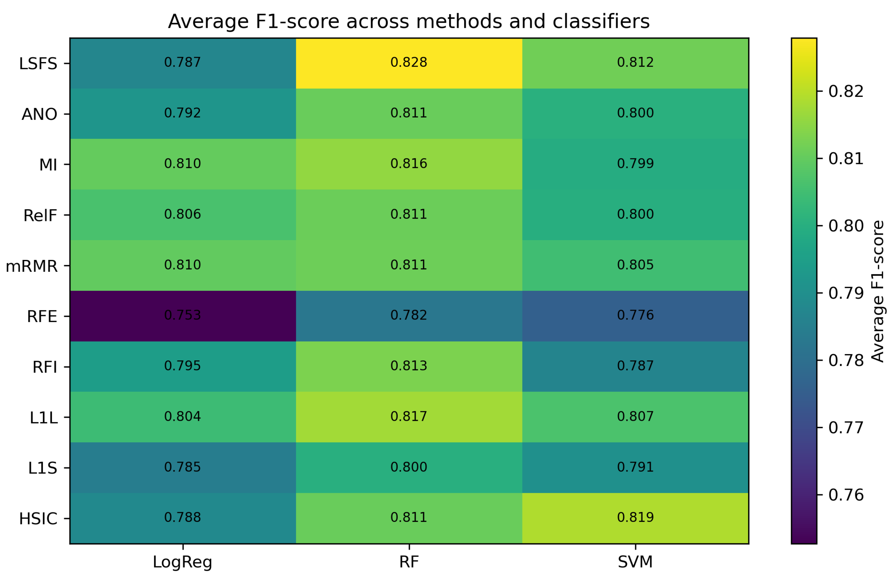
Table 1.
Synthetic binary dataset with 10 features and one label.
| Sample | y | ||||||||||
|---|---|---|---|---|---|---|---|---|---|---|---|
| 1 | 1 | 0 | 1 | 0 | 1 | 0 | 1 | 0 | 0 | 1 | 1 |
| 2 | 1 | 1 | 0 | 0 | 1 | 1 | 0 | 0 | 0 | 1 | 1 |
| 3 | 0 | 1 | 1 | 1 | 0 | 1 | 0 | 0 | 1 | 0 | 0 |
| 4 | 0 | 0 | 1 | 1 | 0 | 0 | 1 | 1 | 0 | 0 | 0 |
| 5 | 1 | 1 | 0 | 0 | 1 | 1 | 0 | 1 | 0 | 1 | 1 |
Table 3.
F1-score comparison using Logistic Regression. Best values per dataset are in bold.
| Dataset | LSFS | ANO | MI | RelF | mRMR | RFE | RFI | L1L | L1S | HSIC |
|---|---|---|---|---|---|---|---|---|---|---|
| ALLAML | 0.908 | 0.920 | 0.912 | 0.920 | 0.920 | 0.938 | 0.919 | 0.938 | 0.938 | 0.905 |
| GLIOMA | 0.654 | 0.650 | 0.650 | 0.650 | 0.650 | 0.470 | 0.650 | 0.453 | 0.453 | 0.671 |
| Prostate | 0.940 | 0.938 | 0.948 | 0.948 | 0.948 | 0.940 | 0.938 | 0.911 | 0.911 | 0.940 |
| SMK_C | 0.716 | 0.733 | 0.734 | 0.688 | 0.726 | 0.703 | 0.720 | 0.733 | 0.733 | 0.723 |
| TOX_171 | 0.974 | 0.982 | 0.976 | 0.976 | 0.969 | 0.994 | 0.974 | 0.975 | 0.975 | 0.975 |
| Colon | 0.496 | 0.718 | 0.688 | 0.769 | 0.688 | 0.652 | 0.718 | 0.657 | 0.657 | 0.604 |
| Leukemia | 0.941 | 0.941 | 0.941 | 0.926 | 0.941 | 0.960 | 0.941 | 0.941 | 0.941 | 0.960 |
| Pixraw10P | 0.962 | 0.794 | 0.947 | 0.837 | 0.946 | 0.777 | 0.895 | 0.987 | 0.987 | 0.898 |
| ARCENE | 0.790 | 0.640 | 0.711 | 0.752 | 0.717 | 0.495 | 0.773 | 0.667 | 0.705 | 0.658 |
| DORO | 0.589 | 0.603 | 0.597 | 0.597 | 0.594 | 0.599 | 0.579 | 0.553 | 0.546 | 0.549 |
Shortened dataset names: Prostate = Prostate_GE, SMK_C = SMK_CAN_187, DORO = DOROTHEA.
Table 4.
F1-score comparison using Random Forest. Best values per dataset are in bold.
| Dataset | LSFS | ANO | MI | RelF | mRMR | RFE | RFI | L1L | L1S | HSIC |
|---|---|---|---|---|---|---|---|---|---|---|
| ALLAML | 0.960 | 0.956 | 0.956 | 0.937 | 0.937 | 0.937 | 0.956 | 0.960 | 0.960 | 0.956 |
| GLIOMA | 0.650 | 0.650 | 0.590 | 0.650 | 0.590 | 0.490 | 0.650 | 0.603 | 0.603 | 0.611 |
| Prostate | 0.938 | 0.926 | 0.926 | 0.918 | 0.926 | 0.928 | 0.926 | 0.909 | 0.909 | 0.928 |
| SMK_C | 0.688 | 0.735 | 0.723 | 0.697 | 0.723 | 0.699 | 0.735 | 0.721 | 0.721 | 0.748 |
| TOX_171 | 0.915 | 0.909 | 0.960 | 0.902 | 0.960 | 0.969 | 0.975 | 0.981 | 0.981 | 0.975 |
| Colon | 0.716 | 0.736 | 0.736 | 0.784 | 0.736 | 0.668 | 0.736 | 0.588 | 0.588 | 0.722 |
| Leukemia | 0.960 | 0.960 | 0.960 | 0.960 | 0.960 | 0.960 | 0.960 | 0.982 | 0.982 | 0.960 |
| Pixraw10P | 0.962 | 0.896 | 0.960 | 0.872 | 0.960 | 0.973 | 0.921 | 0.987 | 0.987 | 0.921 |
| ARCENE | 0.751 | 0.659 | 0.741 | 0.707 | 0.735 | 0.580 | 0.725 | 0.728 | 0.725 | 0.711 |
| DORO | 0.667 | 0.682 | 0.667 | 0.685 | 0.584 | 0.620 | 0.650 | 0.598 | 0.547 | 0.577 |
Shortened dataset names: Prostate = Prostate_GE, SMK_C = SMK_CAN_187, DORO = DOROTHEA.
Table 5.
F1-score comparison using SVM. Best values per dataset are in bold.
| Dataset | LSFS | ANO | MI | RelF | mRMR | RFE | RFI | L1L | L1S | HSIC |
|---|---|---|---|---|---|---|---|---|---|---|
| ALLAML | 0.960 | 0.905 | 0.905 | 0.941 | 0.905 | 0.905 | 0.920 | 0.938 | 0.938 | 0.920 |
| GLIOMA | 0.653 | 0.710 | 0.650 | 0.633 | 0.650 | 0.533 | 0.710 | 0.590 | 0.590 | 0.710 |
| Prostate | 0.937 | 0.926 | 0.937 | 0.937 | 0.937 | 0.940 | 0.926 | 0.920 | 0.920 | 0.940 |
| SMK_C | 0.741 | 0.747 | 0.728 | 0.713 | 0.728 | 0.726 | 0.747 | 0.750 | 0.750 | 0.751 |
| TOX_171 | 0.948 | 0.883 | 0.897 | 0.836 | 0.897 | 0.919 | 0.913 | 0.913 | 0.913 | 0.913 |
| Colon | 0.637 | 0.736 | 0.736 | 0.784 | 0.736 | 0.700 | 0.736 | 0.640 | 0.640 | 0.748 |
| Leukemia | 0.916 | 0.941 | 0.941 | 0.941 | 0.941 | 0.960 | 0.941 | 0.941 | 0.941 | 0.960 |
| Pixraw10P | 0.973 | 0.804 | 0.935 | 0.849 | 0.935 | 0.862 | 0.924 | 1.000 | 1.000 | 0.924 |
| ARCENE | 0.760 | 0.666 | 0.711 | 0.664 | 0.702 | 0.560 | 0.721 | 0.694 | 0.713 | 0.707 |
| DORO | 0.691 | 0.685 | 0.692 | 0.699 | 0.617 | 0.652 | 0.683 | 0.616 | 0.500 | 0.616 |
Shortened dataset names: Prostate = Prostate_GE, SMK_C = SMK_CAN_187, DORO = DOROTHEA.
Table 6.
Average LSFS performance across datasets under multiple evaluation metrics.
| Classifier | Acc. | Bal. Acc. | Precision | Recall | F1 | AUC | MCC |
|---|---|---|---|---|---|---|---|
| LR | 0.862 | 0.840 | 0.799 | 0.810 | 0.797 | 0.897 | 0.686 |
| RF | 0.880 | 0.855 | 0.858 | 0.806 | 0.821 | 0.913 | 0.726 |
| SVM | 0.876 | 0.855 | 0.849 | 0.819 | 0.822 | 0.913 | 0.724 |
Table 7.
Average F1-score across all datasets.
| Method | LR | RF | SVM |
|---|---|---|---|
| LSFS | 0.797 | 0.821 | 0.822 |
| ANO | 0.792 | 0.811 | 0.800 |
| MI | 0.810 | 0.822 | 0.813 |
| RelF | 0.806 | 0.811 | 0.800 |
| mRMR | 0.810 | 0.811 | 0.805 |
| RFE | 0.753 | 0.782 | 0.776 |
| RFI | 0.811 | 0.823 | 0.822 |
| L1L | 0.782 | 0.806 | 0.800 |
| L1S | 0.785 | 0.800 | 0.790 |
| HSIC | 0.788 | 0.811 | 0.819 |
Table 8.
Candidate retrieval efficiency of LSFS.
| Dataset | Original Features | Retrieved Candidates | Reduction Ratio |
|---|---|---|---|
| ALLAML | 7,129 | 252.4 | 96.46% |
| GLIOMA | 4,434 | 1,309.2 | 70.46% |
| Prostate_GE | 5,966 | 1,068.0 | 82.08% |
| SMK_CAN_187 | 19,993 | 3,151.6 | 84.24% |
| TOX_171 | 5,748 | 2,120.4 | 63.11% |
| ARCENE | 10,000 | 291.6 | 97.07% |
| Colon | 2,000 | 185.2 | 90.74% |
| DOROTHEA | 100,000 | 909.0 | 98.97% |
| Leukemia | 7,070 | 726.8 | 89.72% |
| Pixraw10P | 10,000 | 1,747.0 | 82.53% |
| Average | 17,234 | 1,176.1 | 85.54% |
Table 9.
Average LSFS feature selection runtime.
| Dataset | Selection Time (seconds) |
|---|---|
| ALLAML | 6.55 |
| GLIOMA | 4.17 |
| Prostate_GE | 5.78 |
| SMK_CAN_187 | 20.19 |
| TOX_171 | 5.82 |
| ARCENE | 10.39 |
| Colon | 1.93 |
| DOROTHEA | 165.56 |
| Leukemia | 6.79 |
| Pixraw10P | 9.57 |
| Average | 23.67 |
Table 10.
Average ranking of feature selection methods across datasets. Lower is better.
| Method | LR | RF | SVM |
|---|---|---|---|
| LSFS | 5.85 | 4.55 | 4.35 |
| ANO | 5.00 | 5.50 | 6.40 |
| MI | 4.25 | 5.15 | 5.45 |
| RelF | 5.10 | 6.50 | 5.95 |
| mRMR | 5.15 | 6.05 | 6.15 |
| RFE | 5.65 | 6.80 | 6.35 |
| RFI | 5.95 | 4.75 | 4.80 |
| L1L | 5.90 | 4.95 | 6.00 |
| L1S | 6.00 | 5.40 | 5.75 |
| HSIC | 6.15 | 5.35 | 3.80 |
Table 11.
Friedman test results across methods for each classifier.
| Classifier | Friedman Statistic | p-value |
|---|---|---|
| LR | 3.830 | 0.922 |
| RF | 5.894 | 0.750 |
| SVM | 8.425 | 0.492 |
Table 12.
LSFS feature selection stability across datasets.
| Dataset | Stability Score |
|---|---|
| ALLAML | 0.073 |
| GLIOMA | 0.058 |
| Prostate_GE | 0.333 |
| SMK_CAN_187 | 0.029 |
| TOX_171 | 0.242 |
| ARCENE | 0.082 |
| Colon | 0.103 |
| DOROTHEA | 0.553 |
| Leukemia | 0.369 |
| Pixraw10P | 0.195 |
| Average | 0.204 |
Table 13.
Average overlap with LSFS-selected features.
| Method | Overlap with LSFS |
|---|---|
| ANO | 0.157 |
| MI | 0.288 |
| RelF | 0.155 |
| mRMR | 0.153 |
| RFE | 0.085 |
| RFI | 0.159 |
| L1L | 0.071 |
| L1S | 0.052 |
| HSIC | 0.088 |
Disclaimer/Publisher’s Note: The statements, opinions and data contained in all publications are solely those of the individual author(s) and contributor(s) and not of MDPI and/or the editor(s). MDPI and/or the editor(s) disclaim responsibility for any injury to people or property resulting from any ideas, methods, instructions or products referred to in the content. |
© 2026 by the authors. Licensee MDPI, Basel, Switzerland. This article is an open access article distributed under the terms and conditions of the Creative Commons Attribution (CC BY) license (http://creativecommons.org/licenses/by/4.0/).
Copyright: This open access article is published under a Creative Commons CC BY 4.0 license, which permit the free download, distribution, and reuse, provided that the author and preprint are cited in any reuse.


