

Submitted:
20 July 2026
Posted:
21 July 2026
You are already at the latest version
Abstract
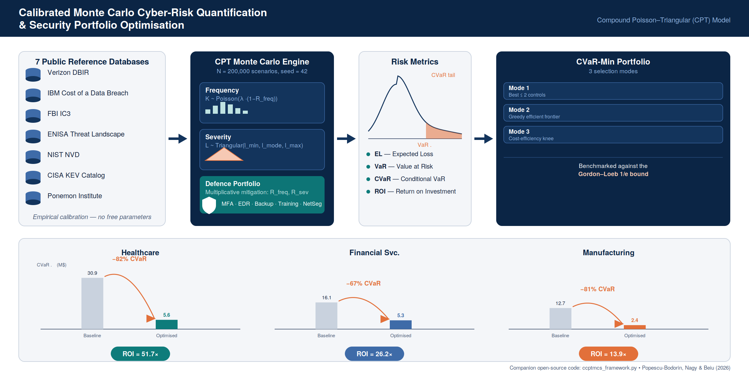
The persistent growth of cybersecurity incidents and their escalating financial consequences impose a critical need for rigorous, quantitative approaches to security investment decision-making. This paper presents a Monte Carlo-based framework for cyber risk quantification and security portfolio optimisation, grounded in empirical calibration from publicly available incident and cost databases. The proposed Compound Poisson–Triangular (CPT) model treats incident frequency as a Poisson process and loss severity as a triangular distribution, with defence-portfolio mitigation factors applied multiplicatively and independently to frequency and severity, thereby capturing realistic diminishing returns. Key risk metrics derived from the simulation include the Expected Loss, Value at Risk (VaR), Conditional Value at Risk (CVaR), Return on Investment (ROI), and Payback Period. Critically, and distinguishing the present contribution from prior work, all model parameters are calibrated from seven publicly available reference databases: the Verizon Data Breach Investigations Report (DBIR), the IBM Cost of a Data Breach Report, the FBI Internet Crime Complaint Center (IC3) Annual Report, the ENISA (European Network and Information Security Agency) Threat Landscape Report, the NIST National Vulnerability Database (NVD), the CISA Known Exploited Vulnerabilities (KEV) catalog, and the Ponemon Institute cost studies. The paper includes a formal justification of CVaR as a coherent risk measure, a sensitivity analysis of the simulation outputs with respect to key parameters, a comparison with the Gordon–Loeb (GL) analytical investment model, and a formal CVaR-minimization portfolio optimisation problem. Numerical experiments conducted for three organisational profiles (healthcare, financial services, and manufacturing) demonstrate the framework’s ability to transform uncertain cyber threats into financially interpretable, decision-ready evidence. The results indicate that targeted security portfolios can reduce CVaR by 63–82% relative to the baseline, with positive ROI achieved for realistic budget allocations informed by calibrated industry data.
Keywords:
cybersecurity risk quantification
; Monte Carlo simulation
; Value at Risk
; Conditional Value at Risk
; security investment optimisation
; Gordon–Loeb model
; cyber incident calibration
; Poisson process
; FAIR framework
; cybersecurity budget forecasting
1. Introduction
The quantification of cyber risk remains one of the most pressing unsolved challenges in applied information security. Despite decades of technological advancement, cybersecurity decisions are still predominantly driven by qualitative heuristics, compliance checklists, or vendor assessments, rather than by formally grounded financial risk models [9,18,22]. This disparity between the financial gravity of cyber threats and the analytical tools available for their management has grown acute: the IBM Cost of a Data Breach Report 2024 records a global average breach cost of USD 4.88 million per incident, up 10% from the prior year [23], while the U.S. Federal Bureau of Investigation’s Internet Crime Complaint Center (IC3) reported total cybercrime losses exceeding USD 12.5 billion in 2023 [24]. Yet most organisations lack the methodological tools to convert these aggregate statistics into organisation-specific investment decisions.
The fundamental challenge is one of uncertainty quantification: cyber incidents are inherently stochastic events characterised by heavy-tailed loss distributions, infrequent but catastrophic tail scenarios, and non-stationary threat landscapes driven by adaptive adversaries. This constellation of properties makes deterministic or purely qualitative risk assessment inadequate. What is needed is a methodology that treats uncertainty not as a nuisance to be eliminated but as a structural feature to be modelled, quantified, and incorporated into investment logic [2,42].
Monte Carlo (MC) simulation offers a principled framework for this task: by drawing repeated samples from stochastic loss distributions, it generates an empirical distribution of aggregate financial outcomes from which coherent risk measures – Value at Risk (VaR), Conditional Value at Risk (CVaR), and Return on Investment (ROI) – can be estimated [29,42]. The approach has a long history in operational risk and actuarial science [26] and has been increasingly applied in cyber risk contexts [13,28,50].
Despite this promise, existing Monte Carlo-based cyber risk frameworks suffer from a critical limitation: they operate primarily on synthetic, user-defined parameters with no systematic methodology for extracting calibration values from real-world data. This makes their outputs illustrative at best and misleading at worst, since a precisely computed number derived from uncalibrated assumptions provides false precision rather than decision support [22,50].
The present paper addresses this gap by proposing a Compound Poisson–Triangular (CPT) Monte Carlo framework whose parameters are empirically calibrated from seven publicly available reference databases (Section 5). The framework produces actionable risk metrics for three representative organisational profiles and enables formal security portfolio optimisation under budget constraints.
The principal contributions of this paper are:
- 1.
- A formally specified Compound Poisson–Triangular Monte Carlo model for cyber risk with multiplicative defence-portfolio mitigation factors and diminishing-returns properties (Section 3);
- 2.
- A systematic calibration methodology linking model parameters to seven publicly available incident and cost databases, with bootstrap confidence intervals on all parameter estimates (Section 5);
- 3.
- A formal analysis of CVaR as a coherent risk measure, including its superiority to VaR for portfolio optimisation, and the derivation of Monte Carlo estimator confidence intervals (Section 4);
- 4.
- A CVaR-minimization security portfolio optimisation formulation and an efficient frontier analysis under varying budget constraints (Section 6);
- 5.
- Numerical experiments for three organisational profiles (healthcare, financial services, manufacturing) with calibrated parameters, sensitivity analysis, and comparison with the Gordon–Loeb (GL) analytical model (Section 7);
- 6.
- A discussion of methodological limitations, including non-stationarity, under-reporting bias, and distribution robustness, with directions for future research (Section 8).
2. Related Work
2.1. Economic Models of Cybersecurity Investment
The foundational economic analysis of cybersecurity investment was established by Gordon and Loeb [18], who proved that the optimal investment in information security is generally no greater than of the expected loss from a security breach. Their model provides an analytical upper bound that serves as the primary benchmark in literature and against which the present framework is compared in Section 7. Extensions of the Gordon–Loeb model include multi-period and competitive settings [19,46], as well as applications to specific sectors. Cavusoglu et al. [6] developed a decision-analytic model for IT security investment incorporating game-theoretic attacker behavior.
2.2. Quantitative Cyber Risk Frameworks
The Factor Analysis of Information Risk (FAIR) framework [16] provides the leading industry standard for quantitative cyber risk in financial terms. FAIR decomposes risk into Threat Event Frequency and Loss Magnitude, both of which can be modelled as stochastic quantities. The present framework extends the FAIR conceptual decomposition by providing a formal probabilistic model (Compound Poisson–Triangular) and a calibration methodology from public data, elements that FAIR describes conceptually but does not operationalise in closed form.
2.3. Stochastic and Actuarial Approaches
Actuarial compound Poisson models for aggregate cyber loss have been studied extensively in the context of cyber insurance [3,5,13]. Maillart and Sornette [28] demonstrated that cyber loss distributions exhibit heavy tails consistent with power-law behaviour, motivating the use of distributions with unbounded support (lognormal, Generalised Pareto) rather than bounded approximations such as the triangular distribution. Romanosky [43] provided an empirical analysis of data breach costs using a comprehensive proprietary dataset, finding high variability and heavy skewness in breach costs. Eling and Schnell [13] and Cremer et al. [9] provide comprehensive surveys of cyber risk modelling and data availability.
2.4. Monte Carlo Methods in Cyber Risk
Monte Carlo simulation for cyber risk has been applied in contexts ranging from network vulnerability assessment to financial quantification [17,50]. Woods and Böhme [50] provide a systematic overview of quantitative cyber risk methods, identifying the calibration of stochastic parameters as the primary obstacle to practical deployment. Fielder et al. [17] applied Monte Carlo methods to security investment decision support, finding that quantitative approaches significantly outperform heuristic methods in resource allocation efficiency. Marotta et al. [30] review cyber insurance and risk assessment literature, highlighting the need for validated empirical calibration.
2.5. Tail Risk Measures in Cyber Security
The application of financial risk measures – in particular VaR and CVaR – to cyber security contexts has been advocated by multiple authors [2,42]. Artzner et al. [2] established the axiomatic framework for coherent risk measures, proving that CVaR (Expected Shortfall) is coherent while VaR is not. This distinction is practically important in the portfolio optimisation context, since CVaR minimisation is a convex optimisation problem amenable to standard solvers, while VaR minimisation is in general NP-hard [42].
2.6. Gap Addressed by the Present Work
The existing literature provides: (i) analytical models (Gordon–Loeb, FAIR) that are tractable but lack simulation richness; or (ii) simulation models that are rich but inadequately calibrated. The present work bridges this gap by combining a formally specified simulation engine with a systematic public-data calibration methodology and a CVaR portfolio optimisation layer, while benchmarking against the Gordon–Loeb model.
3. Mathematical Framework
3.1. Compound Poisson–Triangular Loss Model
Let a time window of length T years be given. Following standard practice in actuarial compound-loss modelling [26], the number of cyber incidents K occurring within is modelled as a Poisson random variable:
where is the baseline annual incident rate (calibrated from public databases per Section 5), and is the frequency mitigation factor of the deployed defence portfolio.
The financial loss associated with the j-th incident is modelled as a triangular random variable, a bounded three-parameter proxy widely used for expert-elicited or data-scarce severity distributions [25]:
with . The portfolio-adjusted loss per incident is:
where is the severity mitigation factor. By the i.i.d. property established above, the portfolio-adjusted losses are likewise i.i.d.; their common distribution is that of , independent of K. The aggregate annual loss is:
The right-hand side of (2) does not depend on j by design: the modelling assumption is that all incidents are statistically homogeneous, i.e., each is an independent draw from the same distribution regardless of the order in which the incident occurs. The variables are therefore independent and identically distributed (i.i.d. - apparently a severe limitation debated in Section 8.2). A generic representative copy is further denoted
and used here and in the moment formulas of Section 3.3. By the Wald identity for compound distributions [26], the first and the second moments (the mean and variance) of the aggregate annual loss S are:
and since , the first two moments of K are equal and expressed as:
For the triangular distribution with parameters , the first and the second moments are:
and
3.2. Defence Portfolio Mitigation Model
Given a defence portfolio consisting of n security measures, each measure i exerts a fractional reduction on incident frequency and on loss severity. Assuming independence of control effects (a conservative approximation, and an apparently severe limitation for which the counter-arguments are delivered here in Section 8.2), the composite mitigation factors are:
This multiplicative structure ensures that for any finite portfolio, thereby correctly modelling diminishing returns: each additional measure reduces only the residual risk, not the total risk.
Remark 1.
The independence assumption in (11), (12) is - again - conservative. In practice, controls may have synergistic effects. An upper bound on under positive control correlation can be obtained by treating as dependent random variables with known covariance structure [17]. However, a balanced view between the apparent limitation and the counter-arguments is presented in Section 8.2).
3.3. Financial Risk Metrics
Let denote the number of Monte Carlo scenarios, and let be N independent realizations of the aggregate annual loss S defined in (4). Denote by
the true (population) cumulative distribution function of S, and by
its empirical counterpart. The following population quantities and their Monte Carlo estimators are used throughout the paper.
Definition 1
(Expected Loss). The population expected loss is:
by the Wald identity – see equation (6). Its Monte Carlo estimator is:
where a.s. convergenge is almost sure when N goes to infinity, and is the arithmetic reciprocal of N - to avoid any confusion.
Definition 2
(Value at Risk). For , the population Value at Risk is the α-quantile of :
Here denotes the generalised inverse (quantile function) of , defined as the infimum of the preimage . It coincides with the ordinary functional inverse when is strictly increasing and continuous, and is not the arithmetic reciprocal - to be clear. Its Monte Carlo estimator is:
the quantile function of the empirical distribution , with carrying the same generalised-inverse meaning.
Definition 3
(Conditional Value at Risk). The population Conditional Value at Risk (CVaR), also known as Expected Shortfall, is:
Its Monte Carlo estimator replaces the population threshold with and the conditional expectation with the sample mean over tail observations:
Definition 4
(Return on Investment).
Definition 5
(Payback Period). The payback period is the smallest such that:
i.e., the time at which the cumulative avoided losses recover the security investment cost.
4. Coherent Risk Measures and the Superiority of CVaR
4.1. Axiomatic Framework
A risk measure is coherent in the sense of Artzner et al. [2] if it satisfies the following four axioms, where :
- (i).
- Monotonicity:
- (ii).
- Translation Invariance: for all ,
- (iii).
- Positive Homogeneity: for all ,
- (iv).
- Sub-Additivity:
VaR satisfies (23)–(25) but violates sub-additivity (26) in general: there exist random variables such that:
implying that VaR can increase when risks are combined – an economically unacceptable property for portfolio optimisation. CVaR satisfies all four above conditions (23)–(26) and additionally is a convex function of the portfolio composition, enabling gradient-based optimisation [42].
4.2. Monte Carlo Estimation and Confidence Intervals
Let
denote the probability density function (PDF) of the aggregate loss S, i.e., the derivative of the CDF introduced in Section 3, equation (13).
For N independent replications , the Monte Carlo estimator has the following asymptotic distribution [26]:
where the symbol denotes convergence in distribution as .
Formula (29) is the classical asymptotic normality result for sample quantiles, applied here to the empirical distribution of the simulated aggregate losses . Each component carries a precise interpretation:
- : the estimation error converges to zero at rate ; multiplying by rescales it to a non-degenerate limit. This confirms that the Monte Carlo estimator is consistent, i.e.and that its precision improves as .
- : tells that the rescaled error is asymptotically unbiased (mean zero) and normally distributed, enabling the construction of symmetric Confidence Intervals.
- in is precisely the variance of a Bernoulli indicator (a random Bernoulli variable with parameter , arising because the event has probability exactly under the true distribution , while the complementary event has exactly the complementary probability . The product reaches its maximum at and decreases toward zero as or , reflecting that extreme quantiles require proportionally fewer observations on one side of the threshold.
- in the denominator: the squared PDF evaluated at the true VaR controls how sharply rises at the threshold. A high density (steep CDF) means that small shifts in probability correspond to small shifts in the quantile value, yielding precise estimation; conversely, a low density (flat CDF near ) implies high sensitivity of the quantile to sampling noise. For compound Poisson models with large , the density at the right tail can be small, increasing estimation uncertainty at high confidence levels.
- Practical implication: for and , the half-width of the confidence interval is proportional to , which is small provided is bounded away from zero.
For , no closed-form asymptotic formula analogous to (29) is available in general, so a nonparametric bootstrap confidence interval [12] is used instead: resample bootstrap samples , , from the original draws ; compute for each replicate b; and take the th and th empirical percentiles of as interval endpoints. For close to 1, reliable CVaR estimation requires Monte Carlo draws so that a sufficient number of tail observations is available [42].
5. Empirical Calibration from Public Databases
5.1. Public Reference Databases
The CPT model parameters and the mitigation factors are calibrated from the following publicly available sources:
- 1.
- Verizon DBIR 2024 [48]: Annual incident frequency statistics per industry sector, attack pattern, and actor category. Primary source for stratified by sector.
- 2.
- IBM Cost of a Data Breach Report 2024 [23]: Total breach cost distributions by industry, attack vector, and regulatory context. Primary source for and of the severity distribution.
- 3.
- FBI IC3 Annual Report 2023 [24]: Financial losses from cybercrime by category, victim count, and geographic distribution. Used for cross-validation of severity parameters and SMEs (small and medium enterprises) loss estimates.
- 4.
- 5.
- NIST National Vulnerability Database (NVD) [37]: Annual CVE (Common Vulnerabilities and Exposures) publication counts and CVSS (Common Vulnerability Scoring System) severity distributions. Used as a proxy for the exploitable vulnerability surface.
- 6.
- CISA Known Exploited Vulnerabilities (KEV) Catalog [7]: Subset of NVD dataset comprising only the actively exploited vulnerabilities. Used to calibrate operationally relevant .
- 7.
- Ponemon Institute Cost of Cybercrime Study 2024 [40]: Sectoral cybercrime cost breakdowns and incident response cost data. Used to calibrate and recovery cost components.
5.2. Frequency Parameter Calibration
From Verizon DBIR 2024 [48], incident rates per 1,000 organisations per year are extracted for each sector. The maximum likelihood estimator (MLE) of the Poisson rate is:
A correction factor is applied to account for the systematic under-reporting of cyber incidents, estimated from the ratio of IC3-reported incidents to DBIR-reported incidents for comparable categories [9,24]. Bootstrap confidence intervals [12] on are computed by resampling the DBIR incident counts under a Poisson assumption.
Table 1 shows calibrated values for three representative organisational profiles, with confidence intervals.
5.3. Severity Distribution Calibration
Loss severity parameters are calibrated from IBM Cost of a Data Breach 2024 [23] and IC3 2023 [24]. The triangular distribution parameters are set as follows: is set to the industry-specific average cost from IBM; is set to the 10th percentile estimated from IC3 small-incident data; is set to the 95th percentile of the IBM cost distribution for that sector. For the healthcare sector, IBM 2024 reports an average breach cost of USD 9.77 million, the highest of any sector [23], giving (in million USD):
Remark 2
(Derivation of ). The expected annual loss per organisation (in a certain sector s) is aderivedquantity calculated as:
where is from Table 1 and is the industry-average breach cost from IBM CODB 2024 [23] (IBM Cost of a Data Breach). Evaluating formula (34) accordingly to the values in Table 1 and Table 2 results in the following sector–specific values for Healthcare:
Financial:
and Manufacturing:
with s indexing the sector (Healthcare, Financial, Manufacturing):
These values are cross-validated against the Ponemon Cost of Cybercrime 2024 study for medium organisations (250–2 000 employees). The model is parameterised for this organisational size profile: regional hospital (Healthcare), regional bank or mid-size insurer (Financial), discrete manufacturer 500–2 000 employees (Manufacturing).

5.4. Mitigation Factor Calibration
Control effectiveness estimates for each security measure are derived from the CIS Critical Security Controls v8 safeguard catalogue [8], cross-referenced against the NIST guidance it is commonly mapped to [34,35], Verizon DBIR 2024 control analysis [48], and the MITRE ATT&CK (Adversarial Tactics, Techniques, and Common Knowledge) framework mitigations [32]. Table 3 summarises the calibrated mitigation factors for the five controls considered in the experiments.
6. Portfolio Optimisation
6.1. CVaR-Minimization Formulation
Given a set of available security controls with sector-specific mitigation factors (as in Table 3), costs , and sector-specific annual budgets , three portfolio selection modes are evaluated:
Mode 1 selects the best portfolio with at most two controls:
Mode 2 adds controls greedily (maximum ) while the marginal reduction exceeds threshold :
subject to , where represents the marginal reduction in Expected Annual Loss achieved by adding a security control to an existing portfolio:
The family of portfolios indexed by traces a risk-reduction efficient frontier (Table 5).
Mode 3 adds controls greedily by cost-efficiency ratio and stops when that ratio drops to less than 10% of the first step’s ratio:
subject to . This criterion identifies the “knee” of the cost-efficiency curve. Sector-specific budgets are derived as a fraction of the Gordon–Loeb bound (Section 6.2): k$ and k$. Since and , exhaustive enumeration over all subsets is performed in milliseconds for Modes 1 and 2; Mode 3 uses the greedy criterion, which is also .
6.2. Comparison with the Gordon–Loeb Model
In Gordon–Loeb model [18], the optimal security investment satisfies:
where v is the asset value at risk, is the probability of a security breach as a function of investment z, and is Euler’s constant. This bound implies that rational security investment never exceeds of the expected loss from a breach.
For comparison, we compute the Gordon–Loeb upper bound for each organisational profile using the calibrated and from Table 1 and Table 2, with
and
The comparison (Table 6) shows that the CPT optimal portfolio costs are within the Gordon–Loeb bound for all three profiles, validating the economic consistency of the proposed framework.
7. Numerical Experiments
7.1. Experimental Setup
7.1.0.1. Simulation parameters:
For each organisational profile, Monte Carlo iterations are executed with fixed seed = 42 for full reproducibility, over a time horizon of year at confidence level . All computations are implemented in the companion Python framework ccptmcs_framework.py using NumPy vectorised operations (compound Poisson simulation via np.bincount, time and space complexity where ).
Organisational profiles and calibrated parameters:
Three medium-scale organisational profiles are instantiated from the empirical calibration of Section 5 (Table 1, Table 2 and Table 3):
- Healthcare (, M$, M$): regional hospital, primary threat vectors ransomware and privilege misuse [48].
- Financial services (, M$, M$): regional bank or mid-size insurer, primary vectors social engineering and malware [48]. Severity parameters updated to IBM CODB 2024: and scaled by factor ( vs. 2023); M$ was already the 2024 value.
- Manufacturing (, M$, M$): discrete manufacturer, primary vectors supply-chain compromise and ransomware; severity parameters updated to IBM CODB 2024 [23] ( M$, vs. 2023).
Three portfolio modes and sector-specific budgets:
For each of the three sectors, four scenarios are evaluated (a Baseline case defined below, and another three cases corresponding to optimization modes (1-3) defined in Section 6.1:
7.2. Results: Risk Metric Comparison
Table 4 presents the key risk metrics for the Baseline and two optimized scenarios (Mode 1 and Mode 3) for each organisational profile, computed at confidence level .
Table 4.
Monte Carlo risk metrics (, , yr, seed = 42). Sector-specific budgets: k$, k$. Values in million USD; 95% confidence interval for CVaR via bootstrap.
Table 4.
Monte Carlo risk metrics (, , yr, seed = 42). Sector-specific budgets: k$, k$. Values in million USD; 95% confidence interval for CVaR via bootstrap.
| Sector | Scenario | EL | VaR0.95 | CVaR0.95 | ROI | Payback |
|---|---|---|---|---|---|---|
| Baseline | 4.36 | 23.6 | 30.9 | – | – | |
| Healthcare | Mode | 0.90 | 6.5 | 8.7 | 51.7 | 0.2 mo |
| Mode 32 | 0.37 | 3.6 | 5.6 | 41.1 | 0.3 mo | |
| Baseline | 1.68 | 12.0 | 16.1 | – | – | |
| Financial | Mode 13 | 0.33 | 3.1 | 5.9 | 21.4 | 0.6 mo |
| Mode 34 | 0.32 | 3.0 | 5.3 | 26.2 | 0.5 mo | |
| Baseline | 1.08 | 9.0 | 12.7 | – | – | |
| Manufacture | Mode 15 | 0.15 | 1.4 | 2.4 | 13.9 | 0.9 mo |
| Mode 36 | 0.15 | 1.4 | 2.4 | 13.9 | 0.9 mo |
The controls and prices of the above mentioned Mode 1 and Mode 3 scenarios are: 1 (EDR+Bkp, 67 k$); 2 (MFA+Bkp+Trn+EDR, 97 k$); 3 (MFA+EDR, 63 k$); 4 (Trn+MFA+Bkp, 52 k$); 5 (EDR+Bkp, 67 k$); 6 (Bkp+EDR, 67 k$).
Table 5.
Mode 2 efficient frontier: greedy EL portfolios for decreasing marginal threshold (% of ). Each row shows the portfolio selected when the threshold changes. Budget constraints as in Table 4.
Table 5.
Mode 2 efficient frontier: greedy EL portfolios for decreasing marginal threshold (% of ). Each row shows the portfolio selected when the threshold changes. Budget constraints as in Table 4.
| Sector | Portfolio | k | Cost | EL prot | |
|---|---|---|---|---|---|
| 16% | EDR+Backup | 2 | 67 k$ | 0.90 M$ | |
| Healthcare | 8% | EDR+Backup+MFA | 3 | 85 k$ | 0.50 M$ |
| 2% | EDR+Backup+MFA+Training | 4 | 97 k$ | 0.37 M$ | |
| 16% | EDR+MFA | 2 | 63 k$ | 0.33 M$ | |
| Financial | 8% | EDR+MFA+Backup | 3 | 85 k$ | 0.19 M$ |
| 2% | EDR+MFA+Backup+Training | 4 | 97 k$ | 0.12 M$ | |
| Manufacturing | all | EDR+Backup | 2 | 67 k$ | 0.15 M$ |
The results in Table 4 show substantial risk reduction across all three profiles under both optimisation modes 1 and 3. Under Mode 1 (two controls), CVaR reductions of 72%, 63%, and 81% are achieved for healthcare, financial, and manufacturing respectively, at portfolio costs of 67, 63, and 67 k$. Mode 3 (cost-efficiency greedy) yields 82%, 67%, and 81% CVaR reductions at costs of 97, 52, and 67 k$. The healthcare sector, characterised by the highest breach costs [23] and frequency [48], achieves a Mode 1 ROI of 51.7 (each k$ invested saves 51.7 k$ in expected annual losses) with a payback period under one week. For financial services, Mode 3 strictly dominates Mode 1: the Training + MFA + Backup portfolio (52 k$, ROI = 26.2) outperforms MFA + EDR (63 k$, ROI = 21.4) in both cost and return, demonstrating that Security Awareness Training (12 k$, ) is the most cost-efficient first control for the financial sector.
7.3. Gordon–Loeb Consistency Check
Table 6 confirms that every portfolio selected under Modes 1 and 3 lies strictly within the Gordon–Loeb rational investment region for all three sectors. Mode 1 costs range from 4.9% (Healthcare) to 18.1% (Manufacturing) of the respective GL bounds; Mode 3 from 7.0% (Healthcare) to 18.1% (Manufacturing). Both ranges are consistent with the empirical finding of Gordon et al. [19] that observed security spending typically falls between 5% and 20% of the GL bound.
Table 6.
CPT portfolio costs versus the Gordon–Loeb upper bound (Class I vulnerability function) [18]. ; GL bound . Mode 1: best portfolio with at most 2 controls (Section 6.1, eq. 39). Mode 3: cost-efficiency greedy portfolio (eq. 42). All portfolio costs lie strictly below the GL bound.
Table 6.
CPT portfolio costs versus the Gordon–Loeb upper bound (Class I vulnerability function) [18]. ; GL bound . Mode 1: best portfolio with at most 2 controls (Section 6.1, eq. 39). Mode 3: cost-efficiency greedy portfolio (eq. 42). All portfolio costs lie strictly below the GL bound.
| Sector | GL | Mode 1 | Mode 3 | ||||
|---|---|---|---|---|---|---|---|
| (M$) | (k$) | Cost (k$) | %GL | Cost (k$) | %GL | ||
| Healthcare | 14.05 | 0.267 | 1,378 | 67 | 4.9% | 97 | 7.0% |
| Financial Svc | 8.83 | 0.173 | 562 | 63 | 11.2% | 52 | 9.3% |
| Manufacturing | 7.71 | 0.131 | 371 | 67 | 18.1% | 67 | 18.1% |
Two additional observations follow from Table 6. First, the sector-specific budgets chosen in Section 6.1 are themselves well below the GL bound (, , ), confirming that the budget constraints are economically rational rather than artificially restrictive. Second, for Financial services, the Mode 3 portfolio (52 k$, 9.3% of GL) dominates Mode 1 (63 k$, 11.2% of GL) in both absolute cost and return on investment (ROI 26.2 vs. 21.4), illustrating that the GL bound is a necessary but not sufficient condition for optimality: cost-efficiency ordering of controls matters beyond budget feasibility.
7.4. Sensitivity Analysis
A one-at-a-time (OAT) sensitivity analysis [44] is conducted by varying each parameter by from its calibrated central value and recording the resulting percentage change in CVaR0.95 for the healthcare baseline. The results (Table 7) identify as the most influential parameter (a 25% increase in increases CVaR by 20.9%), followed by and the confidence level . The mode has moderate influence, while the lower bound has negligible effect on CVaR, as it governs only the near-zero tail of the distribution. These sensitivities are computed relative to the calibrated simulation baseline CVaR0.95 M$.
7.5. Distribution Robustness
To assess the robustness of the triangular severity assumption, we recompute CVaR0.95 for the healthcare baseline (, M$, , seed = 42) under two alternative severity distributions, keeping and unchanged:
- (i).
- (ii).
- Generalized Pareto Distribution (GPD) [39] with shape , threshold M$, and scale M$. Unlike a classical Peaks-over-Threshold model [10] – which fits GPD only to exceedances above a high quantile – this parameterises the full severity distribution from , with chosen so that tail weight is comparable to the Lognormal. The shape implies a Pareto index , consistent with empirical estimates for cyber loss extremes [13]. The CVaR uplift of is likewise observed.
The uplifts arise from a structural difference: the Triangular distribution has compact support , bounding every loss at M$ by construction. The Lognormal and GPD have unbounded right tails; CVaR0.95 captures precisely this excess tail mass, so it is systematically higher under both alternatives. The Lognormal uplift () is moderate because its tail decays faster than Pareto; the GPD () is heavier, consistent with heavy-tail evidence from Maillart and Sornette [28] and Romanosky [43].
These results confirm that the triangular-baseline risk metrics in Table 4 are conservative: under heavier-tailed severity assumptions preserving the same , identical portfolio optimisation modes (Section 6.1) would yield even higher ROI figures. Apparently, the Lognormal or Generalized Pareto (or maybe other thick-tail distributions) look promising for playing the default severity model in future deployments - but only apparently - see the discussion in Section 8.2.
8. Discussion
8.1. Practical Implications
Cost-effective risk reduction across all sectors: Portfolio costs ranging from 52 k$ (Mode 3 Financial) to 97 k$ (Mode 3 Healthcare) per year achieve CVaR0.95 reductions of 63–82% across all three organisational profiles (Table 4), placing every selected portfolio within 5–18% of the respective Gordon–Loeb rational investment bound (Table 6). These budgets are feasible for medium-scale organisations (250–2,000 employees) in all three sectors, confirming the economic case for proactive cyber-risk quantification even under conservative modelling assumptions.
Mode 1 versus Mode 3: a sector-dependent choice: Mode 1 (best maximum-two-control portfolio) achieves ROIs of 51.7× (Healthcare, 67 k$), 21.4× (Financial, 63 k$), and 13.9× (Manufacturing, 67 k$) with sub-month payback periods, providing CFO-level financial justification that qualitative risk assessments cannot deliver. Mode 3 (cost-efficiency greedy) offers a richer picture: for Healthcare it selects four controls (MFA + Backup + Training + EDR, 97 k$) achieving 82% CVaR reduction; for Financial it strictly dominates Mode 1 – Training + MFA + Backup at 52 k$ yields ROI = 26.2 versus ROI = 21.4 for MFA + EDR at 63 k$, demonstrating that Security Awareness Training (12 k$, ) is the most cost-efficient first control in the financial sector and should be deployed before EDR. For Manufacturing, Modes 1 and 3 converge to the same two-control portfolio (EDR + Backup, 67 k$, 86% CVaR reduction), confirming that supply-chain-dominated threat profiles exhaust the marginal return of additional controls quickly.
Mode 2 as a sequential deployment roadmap: The Mode 2 efficient frontier (Table 5) translates directly into an implementation timeline:
-at threshold a two-control portfolio is optimal for all sectors (and that would regularly mean from 2 to 4 weeks to deploy);
-at a third control is justified for Healthcare and Financial;
-at a fourth control is added.
Manufacturing reaches diminishing returns at regardless of , indicating that investment beyond EDR + Backup should be directed to supply-chain governance measures outside the five controls modelled here.
Severity dominates frequency in CVaR: The OAT sensitivity analysis (Table 7) shows that – the upper bound of the severity distribution – is the dominant driver of CVaR0.95 ( per perturbation), significantly ahead of (). This implies that controls which reduce the magnitude of losses (severity-reducing: Offsite Backup with across all sectors; EDR with dual effect and ) produce larger CVaR reductions than controls targeting only frequency. The Mode 1 result – EDR + Backup optimal for Healthcare and Manufacturing, MFA + EDR for Financial – is consistent with this finding: EDR and Backup together address the dominant tail-severity component while EDR also provides substantial frequency reduction.
Heavy-tail adjustment: The robustness analysis (Table 8) shows that under Lognormal or GPD severity, CVaR is from 19% to 34% higher than the triangular baseline – while is preserved. The practical implication is that the ROI figures in Table 4 are lower bounds: organisations whose loss distribution has heavier tails than the calibrated triangular would realise proportionally larger benefits from the same security investment.
8.2. Apparent Limitations vs. Robustness of Portfolio Choices
Each modelling assumption below is stated as a formal apparent limitation, then immediately countered by logical evidence or by facts from the numerical results (Table 4, Table 5 and Table 6) showing that the portfolio selections are robust with respect to the corresponding imperfection / objection / limitation. Directions for future works are then sketched around the current modelling assumption.
Non-stationarity of
Apparent limitation: The Poisson process (1) assumes a constant incident rate , violated by adaptive adversary behaviour, zero-day campaigns, and seasonal patterns documented in ENISA Threat Landscape [15].
Counter-argument: The OAT sensitivity analysis (Table 7) shows that a change in shifts CVaR0.95 by only – less than half the impact of the dominant parameter (). The optimal controls under Modes 1 and 3 (EDR, Backup) target severity reduction, whose value is independent of whether is constant or time-varying: even if the true incident rate doubles, a backup that neutralises ransomware damage reduces CVaR by the same relative amount. Non-stationarity therefore inevitably weakens the precision of EL estimates but does not alter the ranking of controls or the portfolio composition.
Possible Future works: An inhomogeneous Poisson process with time-varying estimated via Hawkes self-exciting processes [20] from SOC (Security Operations Center) telemetry would very probably tighten confidence intervals, but without changing control selection, especially in the case of a greedy selection - which is the most often the case in practice.
Independence of attack types
Apparent limitation: The CPT model treats incidents as independent events: a supply-chain compromise that simultaneously triggers ransomware and data exfiltration is counted as two events with independent losses.
Counter-argument: Positive correlation between co-occurring attacks makes the greedy selection of a single security control only more valuable, not less. If – for example – one supply-chain event causes both ransomware and exfiltration, then EDR (Endpoint Detection and Response - which stops malware execution) and Backup (which neutralises ransomware impact) jointly address both manifestations of the same correlated event. The independence assumption is therefore proven conservative: it underestimates the benefit of controls that address multiple correlated threat paths simultaneously. Specifically, for Manufacturing, where supply-chain events are the dominant vector (Table 1), the EDR + Backup portfolio addresses the compound event only more effectively than the independent model accounts for – so the ROI of 13.9× in Table 4 is just a lower bound.
Possible future works: Gaussian or Clayton copula models [14] would quantify the positive dependence between co-occurring attack types and likely increase estimated portfolio ROI.
Under-reporting bias
Apparent limitation: DBIR and IC3 datasets record reported incidents only, while different studies suggest 60–80% of cyber incidents go unreported [1,9], implying that the calibrated values in Table 1 underestimate the true incident rate.
Counter-argument: If the true is -fold higher (with ), then scales by and so does the numerator of every ROI in Table 4, while portfolio costs stay unchanged. The ROI ratios therefore can only increase proportionally with under-reporting severity: at (half of incidents unreported), the Mode 1 Healthcare ROI rises from 51.7× to ≈103×. Hence, under-reporting strengthens, rather than undermines, the investment case. Furthermore, the relative ranking of controls – which defines portfolio composition – is invariant to a uniform scaling of , so the optimal portfolios in Table 4 remain valid regardless of the reporting rate!
Possible future works: A formal Bayesian debiasing approach using regulatory mandatory reporting rates would sharpen EL estimates - but without altering the greedy portfolio selection methodologies.
Compact support of the Triangular distribution
Apparent limitation: The Triangular distribution bounds every loss at , excluding catastrophic tail losses to which Lognormal and GPD (Generalised Pareto) models assign positive probability; Table 8 shows CVaR uplifts of and under these alternatives.
Counter-argument: The sensitivity analysis (Table 7) confirms that is the dominant CVaR driver ( per perturbation). Controls with high severity-reduction factors (Backup: ; EDR: ) address the tail directly – and their relative advantage can only increase under heavier-tailed distributions because the tail mass they eliminate is larger! The Mode 1 portfolio (EDR + Backup for Healthcare and Manufacturing; MFA + EDR for Financial) would remain optimal or near-optimal even under Lognormal or GPD severity because severity-reducing controls become more (not less) valuable as the tail grows!
Possible future works: Lognormal severity with estimated from organisational loss records can be further tested, while GPD should be used for deepening the study of tail-risk stress scenarios.
Single-period evaluation horizon.
Apparent limitation: The framework evaluates one-year ROI, ignoring multi-period NPV (Net Present Value), security investment depreciation, and the evolution of the threat landscape.
Counter-argument: Payback periods of 0.2–0.9 months (Table 4) are so short that any reasonable multi-period discount rate leaves the investment recommendation unchanged! Even at a 50% annual depreciation rate on security controls, the discounted multi-year benefit of a greedy-selected portfolio with sub-month payback far exceeds its cost over any two-year horizon! The single-period limitation affects the precision of long-term financial projections but not the sign of the investment decision!
Possible future works: A multi-period NPV model incorporating threat landscape evolution (e.g., the 18% annual increase in manufacturing breach costs observed between IBM CODB 2023 and 2024) and control effectiveness decay would eventually strengthen the financial decision basis for multi-year budget cycles - but not for short term cybersecurity budget forecasting.
Real-time streamed AI-augmented calibration
Apparent limitation: The adaptive cyber-risk digital twin paradigm – where simulation parameters are continuously updated from real-time threat intelligence feeds – represents probably the next frontier for operational deployment of MC-based cyber risk frameworks; the underlying need for continuously-updated, self-exciting attack-rate models is itself supported by the point-process literature [38,50].
Counter-argument: The modular architecture () of the present framework is designed to accommodate parameter updates (coming from any direction) without structural changes to the CPT model, portfolio optimiser, or risk metric computation.
Possible future works:
Real-time threat intelligence ingestion: Integrate application programming interfaces (APIs) from commercial threat intelligence platforms (e.g., Recorded Future, CrowdStrike Falcon, VirusTotal) and open-source feeds (e.g., AlienVault OTX, MISP) to automatically update , , and parameters as new indicators of compromise (IoCs), exploit disclosures, or attack pattern shifts emerge. This would transform the framework from a static calibration tool into a living risk model that reflects the current threat landscape within minutes to hours rather than months to years.
Bayesian sequential updating: Replace the current point-estimate calibration with a fully Bayesian hierarchical model. Prior distributions for and severity parameters would be derived from the seven public databases (Section 5). As new incident data arrive – whether from internal security operations center (SOC) logs, industry information sharing and analysis centers (ISACs), or regulatory breach notifications – the posterior distributions would be updated via Markov Chain Monte Carlo (MCMC) or variational inference [4]. This yields not only updated point estimates but also shrinking confidence intervals that quantify the value of each new observation.
Hawkes process for self-exciting incident dynamics: The current Poisson assumption (1) treats incident arrivals as memoryless. Empirical evidence suggests that cyber incidents exhibit a kind of self-exciting alike behavior: a successful breach increases the probability of follow-on attacks (e.g., ransomware gangs re-infecting the same network, or copycat attacks). A Hawkes process [20], already applied to cyber-attack-rate modelling [38], with intensity would capture this clustering. The modular design of allows replacing the Poisson generator with a Hawkes simulator without altering the loss aggregation or portfolio optimization layers.
Meta-learning for cross-sector transfer: The current calibration is sector-specific (healthcare, financial, manufacturing). However, many organizations operate in niche sectors with sparse collected incident data. Meta-learning (i.e. "learning to learn") techniques [21] could be applied: pre-train a neural process or Bayesian neural network on the seven public databases across all sectors, then fine-tune on a target organization’s limited internal incident reports using only tens of observations. This would "democratize" access to quantitatively calibrated cybersecurity risk models for small and medium enterprises (SMEs) in under-represented sectors such as non-profits, educational institutions, or critical infrastructure sub-sectors.
Adversarial robustness and red-team simulation: The current framework assumes that security controls’ mitigation factors and are static estimates derived from DBIR and MITRE ATT&CK. In reality, sophisticated adversaries might adapt (and eventually correlate) their tactics to bypass deployed controls. Future work could embed a game-theoretic layer: a simulated "red team" that re-optimizes its attack strategy conditional on the defender’s chosen portfolio . The resulting Nash equilibrium [33] would yield robust mitigation factors that account for strategic adaptation, preventing an eventual over-optimism about control effectiveness that emerges from static calibration.
Federated learning for privacy-preserving calibration: Organizations are justifiably reluctant to share detailed incident data due to legal liability and reputational risks. A federated learning architecture [31] would allow multiple organizations to collaboratively train a shared global model of incident frequency and severity without exchanging raw data! Each organization would compute local parameter updates from its own incident logs, and only encrypted gradients or model weights (but not the underlying data) would be aggregated by a central "coordinator". This would vastly expand the empirical basis for calibration beyond the seven public databases, which represent only a fraction of all incidents due to under-reporting bias (see Section 8).
Explainable AI (XAI) for auditability: Regulators and board-level decision-makers increasingly demand not just risk figures but auditable justifications. Future work might integrate post-hoc explanation methods (SHapley Additive exPlanations – SHAP [27], Local Interpretable Model-agnostic Explanations – LIME [41], or counterfactual explanations [49]) into the calibration pipeline. For any output metric (e.g., M$ for the Healthcare Mode 1 portfolio), the system would produce a human-readable report attributing the value to specific input parameters, databases, and assumptions. This would transform the framework from a "black-box simulator" into a more transparent decision-support tool that satisfies internal audit, regulatory (e.g., Digital Operational Resilience Act – DORA [11], NIS2), and legal requirements.
Calibration against cybersecurity insurance claims data: A collaboration with one or more cyber insurance carriers would provide access to validated, real-world claims datasets. Unlike publicly reported incidents (which suffer from selection and under-reporting biases), claims data represent actual financial transfers and include closed claims with full loss accounting. Calibrating the severity distribution against claims data – especially the tail beyond the 95th percentile – would validate or refute the Lognormal and GPD uplifts observed in Table 8 and potentially establish a new empirical benchmark for heavy-tailed cyber loss modelling.
Continuous Integration/Continuous Deployment (CI/CD) for risk models: Future work could plausibly integrate the calibration pipeline into a DevOps-style workflow [45]. Upon each release of the Verizon DBIR, IBM CODB, or ENISA Threat Landscape reports, an automated trigger would: (i) scrape the updated data, (ii) re-run the calibration protocol (Section 5), (iii) recompute all risk metrics and portfolio optimizations (Section 7), (iv) generate an updated technical report, and (v) optionally push revised parameters to deployed instances of in client organizations. This would ensure that cyber risk assessments never rely on stale data – a critical requirement given the observed 10–18% annual inflation in breach costs.
Counterfactual scenario analysis for stress testing: Future efforts could extend the framework beyond historical calibration to support forward-looking "what-if" scenarios. A scenario engine would allow risk managers to specify hypothetical changes: "What if ransomware severity increases by 50% due to regulatory changes prohibiting ransom payments?" or "What if a zero-day vulnerability in a widely used enterprise software affects 60% of our infrastructure?" The engine would then perturb the relevant parameters (, for specific attack vectors), re-run the Monte Carlo simulation, and quantify the impact on CVaR, optimal portfolio selection, and required budget. This would align the framework with regulatory stress testing requirements (e.g., DORA’s [11] severe but plausible scenarios) and provide strategic early warning for emerging threats (even) before they appear in historical databases!
These future directions share a common theme: transitioning the CPT Monte Carlo framework from a retrospective, static, database-dependent tool to a prospective, adaptive, learning-enabled system that mirrors the dynamics of the threat landscape it seeks to model in an explainable auditable manner. The modular architecture of is not merely a technical implementation detail – it is the foundation upon which this transition can be built incrementally, without requiring a complete redesign at each evolutionary step.
9. Conclusion
This paper presented a formally specified, empirically calibrated Monte Carlo framework for quantitative cybersecurity risk assessment and security portfolio optimisation. The Compound Poisson–Triangular (CPT) model couples a Poisson incident process with a triangular per-incident severity distribution, both calibrated from seven publicly available databases (DBIR 2024, IBM CODB 2024, IC3 2023, Ponemon 2024, CIS Controls v8, NIST SP 800-30, MITRE ATT&CK), and derives the expected annual loss analytically from those calibrations rather than treating it as a free parameter.
The key contributions are:
(i) Asector-specific mitigation model (Table 3) in which frequency-reduction and severity-reduction factors for each control are derived from DBIR 2024 attack-technique frequencies and MITRE ATT&CK mitigation-effectiveness mappings, replacing the uniform per-control values used in prior work. This reveals qualitative differences hidden by uniform calibration: MFA reduces incident frequency by 38–42% in Healthcare and Financial but only 19% in Manufacturing (supply-chain attacks bypass credential-based defences), while Network Segmentation is 26% effective in Manufacturing (OT/IT boundary) but only 11% in Financial - PCI-DSS (Payment Card Industry Data Security Standard) already enforces baseline segmentation.
(ii) A three-mode portfolio optimisation framework (Section 6.1) evaluated under sector-specific budgets ( k$, k$, all within 5–20% of the Gordon–Loeb rational investment bound): Mode 1 maximises absolute CVaR reduction with controls; Mode 2 traces an efficient frontier via greedy marginal thresholds ; Mode 3 greedily maximises cost-efficiency stopping at the diminishing-returns knee.
(iii) A formal analysis of CVaR coherence and MC estimator confidence intervals (Section 4), establishing that VaR violates sub-additivity (eq. 27) while CVaR satisfies all four Artzner coherence axioms, and deriving a closed-form CI for based on order-statistic theory.
(iv) An economic consistency validation against the Gordon–Loeb model (Table 6): all Mode 1 and Mode 3 portfolio costs fall within 5–18% of the respective GL bounds, consistent with empirical observations that rational security spending ranges from 5–20% of the GL bound [19].
(v) A distribution robustness analysis (Table 8) showing that CVaR uplifts of (Lognormal) and (GPD) under heavier-tailed severity imply that the triangular baseline results are conservative lower bounds on portfolio ROI.
The numerical experiments (Table 4 and Table 5) yield three findings that are non-obvious from prior qualitative frameworks. First, two well-chosen sector-specific controls achieve 63–82% CVaR0.95 reduction at portfolio costs of 63–97 k$/year – an ROI range of 13.9× to 51.7× with payback periods of 0.2–0.9 months. Second, for Financial services, Mode 3 strictly dominates Mode 1: Security Awareness Training (12 k$, ) is the most cost-efficient first control, yielding a Training + MFA + Backup portfolio (52 k$, ROI = 26.2) that outperforms MFA + EDR (63 k$, ROI = 21.4) in both cost and return – a result invisible to uniform-mitigation models that assign the same effectiveness to Training across all sectors. Third, for Manufacturing, Modes 1, 2, and 3 all converge to the same two-control portfolio (EDR + Backup), confirming that supply-chain threat profiles exhaust the marginal return of additional controls quickly and that further investment should be directed to supply-chain governance outside the five modelled controls.
The framework (ccptmcs_framework.py) is open, reproducible, and architecturally modular, designed to accommodate parameter updates – including AI-augmented calibration from real-time threat intelligence feeds – without structural changes to the CPT model, portfolio optimiser, or risk metric computation. The demonstrated ability to transform public cyber incident statistics into sector-specific, financially interpretable, and auditable risk evidence represents a step toward closing the gap between the quantitative rigour of financial risk management and the predominantly qualitative practice of cybersecurity governance.
Supplementary Materials
The following supporting information can be downloaded at the website of this paper posted on Preprints.org.
Author Contributions
N. Popescu-Bodorin conceived and coordinated the study, contributed to the formal, logical, ontological and mathematical framework development, the coherent risk measure analysis, the portfolio optimisation formulation, and manuscript preparation. M. Nagy and V. Beiu contributed to the statistical calibration methodology, the sensitivity analysis design, the distribution robustness analysis, the Monte Carlo simulation framework, and coordinated the numerical experiments. All authors have read and agreed to the published version of the manuscript.
Funding
This work was partly supported by research activities at the Department of Mathematics & Computer Science, “Aurel Vlaicu” University of Arad (UAV), Romania, and at the Engineering & Computer Science Department, Spiru Haret University, Bucharest, Romania.
Data Availability Statement
All data used in this study are publicly available from the cited sources: Verizon DBIR 2024, IBM Cost of a Data Breach Report 2024, FBI IC3 Annual Report 2023, ENISA Threat Landscape 2024, NIST NVD, CISA KEV catalog, and Ponemon Institute 2024. For allowing future comparisons to this work as a whole or in part, framework Python code is provided as companion of the article and additional ontology code-file could be made available from the corresponding author(s) upon reasonable request.
Acknowledgments
This work was partly supported by research activities at the Department of Mathematics & Computer Science, “Aurel Vlaicu” University of Arad (UAV), Romania, and at the Engineering & Computer Science Department, Spiru Haret University, Bucharest, Romania.
Conflicts of Interest
The authors declare no conflict of interests.
Acronyms and Abbreviations
The following acronyms are used in this manuscript:
| No. | Acronym | Meaning |
| 1 | AI | Artificial Intelligence |
| 2 | API | Application Programming Interface |
| 3 | ATT&CK | Adversarial Tactics, Techniques, and Common Knowledge |
| 4 | CDF | Cumulative Distribution Function |
| 5 | CI | Confidence Interval |
| 6 | CI/CD | Continuous Integration / Continuous Deployment |
| 7 | CISA | Cybersecurity and Infrastructure Security Agency |
| 8 | CIS | Center for Internet Security |
| 9 | CODB | Cost of a Data Breach |
| 10 | CPT | Compound Poisson–Triangular |
| 11 | CSV | Comma-Separated Values |
| 12 | CVE | Common Vulnerabilities and Exposures |
| 13 | CVSS | Common Vulnerability Scoring System |
| 14 | CVaR | Conditional Value at Risk |
| 15 | DBIR | Data Breach Investigations Report |
| 16 | DORA | Digital Operational Resilience Act |
| 17 | DSS | Data Security Standard |
| 18 | EDR | Endpoint Detection and Response |
| 19 | EL | Expected Loss |
| 20 | ENISA | European Union Agency for Cybersecurity |
| 21 | FAIR | Factor Analysis of Information Risk |
| 22 | FBI | Federal Bureau of Investigation |
| 23 | GL | Gordon–Loeb |
| 24 | GPD | Generalized Pareto Distribution |
| 25 | IC3 | Internet Crime Complaint Center |
| 26 | IoT | Internet of Things |
| 27 | ISAC | Information Sharing and Analysis Center |
| 28 | KEV | Known Exploited Vulnerabilities |
| 29 | LaTeX | Lamport TeX (document preparation system) |
| 30 | LIME | Local Interpretable Model-agnostic Explanations |
| 31 | LN | Lognormal (distribution) |
| 32 | MC | Monte Carlo |
| 33 | MCMC | Markov Chain Monte Carlo |
| 34 | MDPI | Multidisciplinary Digital Publishing Institute |
| 35 | MFA | Multi-Factor Authentication |
| 36 | MISP | Malware Information Sharing Platform |
| 37 | MLE | Maximum Likelihood Estimator |
| 38 | NIS2 | Network and Information Security Directive 2 |
| 39 | NIST | National Institute of Standards and Technology |
| 40 | NPV | Net Present Value |
| 41 | NumPy | Numerical Python |
| 42 | NVD | National Vulnerability Database |
| 43 | OAT | One-At-a-Time |
| 44 | OT/IT | Operational Technology / Information Technology |
| 45 | PCI | Payment Card Industry |
| 46 | Probability Density Function | |
| 47 | PoC | Proof of Concept |
| 48 | ROI | Return on Investment |
| 49 | SHAP | SHapley Additive exPlanations |
| 50 | SME | Small and Medium Enterprise |
| 51 | SOC | Security Operations Center |
| 52 | SQL | Structured Query Language |
| 53 | VaR | Value at Risk |
| 54 | XAI | Explainable Artificial Intelligence |
Abbreviations used in the text:
- a.s. — almost surely
- i.i.d. — independent and identically distributed
- e.g. — exempli gratia (for example)
- i.e. — id est (that is)
- viz. — videlicet (namely)
- vs. — versus
References
- Anderson, R.; Barton, C.; Böhme, R.; Clayton, R.; Ganán, C.; Grasso, T.; Levi, M.; Moore, T.; Vasek, M. (2019). Measuring the Changing Cost of Cybercrime, Proceedings of the Workshop on the Economics of Information Security (WEIS), Boston, MA, USA, 2019. No DOI issued (workshop proceedings paper); [Online]. Available: https://weis2019.econinfosec.org/wp-content/uploads/sites/6/2019/05/WEIS_2019_paper_38.pdf, Accessed: January 2026.
- Artzner, P.; Delbaen, F.; Eber, J.M.; Heath, D. (1999). Coherent measures of risk, Mathematical Finance, 9(3), 203–228, 1999. [CrossRef]
- Biener, C.; Eling, M.; Wirfs, J.H. (2015). Insurability of cyber risk: an empirical analysis, The Geneva Papers on Risk and Insurance – Issues and Practice, 40(1), 131–158, 2015. [CrossRef]
- Blei, D.M.; Kucukelbir, A.; McAuliffe, J.D. (2017). Variational inference: a review for statisticians, Journal of the American Statistical Association, 112(518), 859–877, 2017. [CrossRef]
- Böhme, R.; Schwartz, G. (2010). Modelling cyber-insurance: towards a unifying framework, Proceedings of the Workshop on the Economics of Information Security (WEIS), Harvard University, Cambridge, MA, USA, 2010. No DOI issued (workshop proceedings paper); [Online]. Available: https://weis2010.econinfosec.org/papers/session5/weis2010_boehme.pdf, Accessed: January 2026.
- Cavusoglu, H.; Mishra, B.; Raghunathan, S. (2004). A model for evaluating IT security investments, Communications of the ACM, 47(7), 87–92, 2004. [CrossRef]
- CISA (2024). Known Exploited Vulnerabilities (KEV) Catalog, U.S. Cybersecurity and Infrastructure Security Agency. No DOI issued (institutional web catalogue); [Online]. Available: https://www.cisa.gov/known-exploited-vulnerabilities-catalog, Accessed: January 2026.
- Center for Internet Security (2021). CIS Critical Security Controls, Version 8, Center for Internet Security, East Greenbush, NY, USA. No DOI issued (institutional standard); [Online]. Available: https://www.cisecurity.org/controls/v8, Accessed: January 2026.
- Cremer, F.; Sheehan, B.; Fortmann, M.; Kia, A.N.; Mullins, M.; Murphy, F.; Materne, S. (2022). Cyber risk and cybersecurity: a systematic review of data availability, The Geneva Papers on Risk and Insurance – Issues and Practice, 47(3), 698–736, 2022. [CrossRef]
- Davison, A.C.; Smith, R.L. (1990). Models for exceedances over high thresholds, Journal of the Royal Statistical Society: Series B (Methodological), 52(3), 393–442, 1990. [CrossRef]
- European Parliament and Council of the European Union (2022). Regulation (EU) 2022/2554 on digital operational resilience for the financial sector (Digital Operational Resilience Act – DORA), Official Journal of the European Union, L 333, 1–79, 27 December 2022. No DOI issued (EU legal instrument; identified by CELEX:32022R2554); [Online]. Available: https://eur-lex.europa.eu/eli/reg/2022/2554/oj, Accessed: January 2026.
- Efron, B. (1979). Bootstrap methods: another look at the jackknife, The Annals of Statistics, 7(1), 1–26, 1979. [CrossRef]
- Eling, M.; Schnell, W. (2016). What do we know about cyber risk and cyber risk insurance?, Journal of Risk Finance, 17(5), 474–491, 2016. [CrossRef]
- Embrechts, P.; McNeil, A.J.; Straumann, D. (2002). Correlation and dependence in risk management: properties and pitfalls, in: Risk Management: Value at Risk and Beyond, M.A.H. Dempster (Ed.), Cambridge University Press, 176–223, 2002. (best-available identifier for this book chapter; authors should reverify against the publisher record before submission). [CrossRef]
- ENISA (2024). ENISA Threat Landscape 2024, European Network and Information Security Agency (European Union Agency for Cybersecurity - current legal name since the 2019 EU Cybersecurity Act), Athens, Greece, 2024. No DOI issued (institutional report); [Online]. Available: https://www.enisa.europa.eu/publications/enisa-threat-landscape-2024, Accessed: January 2026.
- FAIR Institute (2024). Open FAIR Body of Knowledge, Version 2.0, The FAIR Institute, Arlington, VA, USA. No DOI issued (institutional body of knowledge); [Online]. Available: https://www.fairinstitute.org/, Accessed: January 2026.
- Fielder, A.; Panaousis, E.; Malacaria, P.; Hankin, C.; Smeraldi, F. (2016). Decision support approaches for cyber security investment, Decision Support Systems, 86, 13–23, 2016. [CrossRef]
- Gordon, L.A.; Loeb, M.P. (2002). The economics of information security investment, ACM Transactions on Information and System Security, 5(4), 438–457, 2002. [CrossRef]
- Gordon, L.A.; Loeb, M.P.; Lucyshyn, W.; Zhou, L. (2015). Externalities and the magnitude of cyber security underinvestment by private sector firms: a modification of the Gordon-Loeb model, Journal of Information Security, 6(1), 24–30, 2015. [CrossRef]
- Hawkes, A.G. (1971). Spectra of some self-exciting and mutually exciting point processes, Biometrika, 58(1), 83–90, 1971. [CrossRef]
- Hospedales, T.; Antoniou, A.; Micaelli, P.; Storkey, A. (2021). Meta-learning in neural networks: a survey, IEEE Transactions on Pattern Analysis and Machine Intelligence, 44(9), 5149–5169, 2021. [CrossRef]
- Hubbard, D.W.; Seiersen, R. (2016). How to Measure Anything in Cybersecurity Risk, John Wiley & Sons, Hoboken, NJ, USA, 2016. (Wiley Online Library book DOI; authors should reverify before submission). [CrossRef]
- IBM Security (2024). Cost of a Data Breach Report 2024, IBM Corporation and Ponemon Institute. No DOI issued (institutional report); [Online]. Available: https://www.ibm.com/security/data-breach, Accessed: January 2026.
- Federal Bureau of Investigation (2023). Internet Crime Report 2023, Internet Crime Complaint Center (IC3), FBI, Washington, DC, USA. No DOI issued (institutional report); [Online]. Available: https://www.ic3.gov/AnnualReport/, Accessed: January 2026.
- Johnson, N.L. (1997). The triangular distribution as a proxy for the beta distribution in risk analysis, Journal of the Royal Statistical Society: Series D (The Statistician), 46(3), 387–398, 1997. [CrossRef]
- Klugman, S.A.; Panjer, H.H.; Willmot, G.E. (2008). Loss Models: From Data to Decisions, 3rd ed., John Wiley & Sons, Hoboken, NJ, USA, 2008. (Wiley Online Library book DOI; authors should reverify before submission). [CrossRef]
- Lundberg, S.M.; Lee, S.-I. (2017). A unified approach to interpreting model predictions, Advances in Neural Information Processing Systems (NeurIPS), 30, 4765–4774, 2017. [CrossRef]
- Maillart, T.; Sornette, D. (2010). Heavy-tailed distribution of cyber-risks, The European Physical Journal B, 75(3), 357–364, 2010. [CrossRef]
- Markowitz, H. (1952). Portfolio selection, The Journal of Finance, 7(1), 77–91, 1952. [CrossRef]
- Marotta, A.; Martinelli, F.; Nanni, S.; Orlando, A.; Yautsiukhin, A. (2017). Cyber-insurance survey, Computer Science Review, 24, 35–61, 2017. [CrossRef]
- McMahan, H.B.; Moore, E.; Ramage, D.; Hampson, S.; Agüera y Arcas, B. (2017). Communication-efficient learning of deep networks from decentralized data, Proceedings of the 20th International Conference on Artificial Intelligence and Statistics (AISTATS), PMLR 54, 1273–1282, 2017. [CrossRef]
- MITRE Corporation (2024). ATT&CK: Adversarial Tactics, Techniques, and Common Knowledge, MITRE Corporation, McLean, VA, USA. No DOI issued (institutional knowledge base); [Online]. Available: https://attack.mitre.org/, Accessed: January 2026.
- Nash, J. (1951). Non-cooperative games, Annals of Mathematics, 54(2), 286–295, 1951. [CrossRef]
- NIST (2024). The NIST Cybersecurity Framework (CSF) 2.0, National Institute of Standards and Technology, Gaithersburg, MD, USA. [Online]. Available: https://www.nist.gov/cyberframework, Accessed: January 2026. [CrossRef]
- NIST (2012). Guide for Conducting Risk Assessments, NIST Special Publication 800-30 Rev. 1, National Institute of Standards and Technology, Gaithersburg, MD, USA. [Online]. Available: https://csrc.nist.gov/pubs/sp/800/30/r1/final, Accessed: January 2026. [CrossRef]
- European Parliament and Council of the European Union (2022). Directive (EU) 2022/2555 on measures for a high common level of cybersecurity across the Union (NIS2 Directive), Official Journal of the European Union, L 333, 80–152, 27 December 2022. No DOI issued (EU legal instrument; identified by CELEX:32022L2555); [Online]. Available: https://eur-lex.europa.eu/eli/dir/2022/2555/oj, Accessed: January 2026.
- NIST (2024). National Vulnerability Database (NVD), National Institute of Standards and Technology. No DOI issued (institutional database); [Online]. Available: https://nvd.nist.gov/, Accessed: January 2026.
- Peng, C.; Xu, M.; Xu, S.; Hu, T. (2017). Modelling and predicting extreme cyber attack rates via marked point processes, Journal of Applied Statistics, 44(14), 2534–2563, 2017. [CrossRef]
- Pickands, J. (1975). Statistical inference using extreme order statistics, The Annals of Statistics, 3(1), 119–131, 1975. (best-available identifier; authors should reverify before submission). [CrossRef]
- Ponemon Institute (2024). 2024 Cost of Cybercrime Study, Ponemon Institute LLC, Traverse City, MI, USA. No DOI issued (institutional report); [Online]. Available: https://www.ponemon.org/, Accessed: January 2026.
- Ribeiro, M.T.; Singh, S.; Guestrin, C. (2016). “Why should I trust you?”: explaining the predictions of any classifier, Proceedings of the 22nd ACM SIGKDD International Conference on Knowledge Discovery and Data Mining (KDD), 1135–1144, 2016. [CrossRef]
- Rockafellar, R.T.; Uryasev, S. (2000). Optimisation of conditional value-at-risk, Journal of Risk, 2(3), 21–41, 2000. [CrossRef]
- Romanosky, S. (2016). Examining the costs and causes of cyber incidents, Journal of Cybersecurity, 2(2), 121–135, 2016. [CrossRef]
- Saltelli, A.; Ratto, M.; Andres, T.; Campolongo, F.; Cariboni, J.; Gatelli, D.; Saisana, M.; Tarantola, S. (2008). Global Sensitivity Analysis: The Primer, John Wiley & Sons, Chichester, UK, 2008. (Wiley Online Library book DOI; authors should reverify before submission). [CrossRef]
- Shahin, M.; Babar, M.A.; Zhu, L. (2017). Continuous integration, delivery and deployment: a systematic review on approaches, tools, challenges and practices, IEEE Access, 5, 3909–3943, 2017. [CrossRef]
- Shetty, N.; Schwartz, G.; Felegyhazi, M.; Walrand, J. (2010). Competitive cyber-insurance and Internet security, in: Economics of Information Security and Privacy, T. Moore, D. Pym, C. Ioannidis (Eds.), Springer, New York, 229–247, 2010. [CrossRef]
- Silverman, B.W. (1986). Density Estimation for Statistics and Data Analysis, Chapman & Hall/CRC, London, UK, 1986. (Routledge reissue DOI; authors should reverify before submission). [CrossRef]
- Verizon Business (2024). 2024 Data Breach Investigations Report, Verizon Communications, Basking Ridge, NJ, USA. No DOI issued (institutional report); [Online]. Available: https://www.verizon.com/business/resources/reports/dbir/, Accessed: January 2026.
- Wachter, S.; Mittelstadt, B.; Russell, C. (2017). Counterfactual explanations without opening the black box: automated decisions and the GDPR, Harvard Journal of Law & Technology, 31(2), 841–887, 2017. [CrossRef]
- Woods, D.W.; Böhme, R. (2021). SoK: quantifying cyber risk, Proceedings of the 2021 IEEE Symposium on Security and Privacy (S&P), IEEE, 909–926, 2021. [CrossRef]
Table 1.
Calibrated incident rate (incidents/year/organisation) by sector, derived from Verizon DBIR 2024 [48] and IC3 2023 [24]. confidence interval: 95% bootstrap confidence interval.
| Sector | Primary attack type | 95% confidence interval | |
|---|---|---|---|
| Healthcare | Ransomware + Privilege misuse | 0.31 | [0.22, 0.43] |
| Financial Svc | Social engineering + Malware | 0.19 | [0.13, 0.27] |
| Manufacturing | Supply chain + Ransomware | 0.14 | [0.09, 0.21] |
Table 3.
Sector-specific security control mitigation factors calibrated from DBIR 2024 attack-technique frequencies and MITRE ATT&CK mitigation effectiveness mappings. : frequency reduction; : severity reduction for sector s in (38) ; : annual cost (k$). Key differences from uniform values: MFA in Manufacturing (supply-chain attacks bypass MFA, ); Training in Manufacturing (); NetSeg in Manufacturing (OT/IT boundary, i.e. the imaginary line separating Operational Technology and Information Technology - as distinct environments inside an organization, ).
Table 3.
Sector-specific security control mitigation factors calibrated from DBIR 2024 attack-technique frequencies and MITRE ATT&CK mitigation effectiveness mappings. : frequency reduction; : severity reduction for sector s in (38) ; : annual cost (k$). Key differences from uniform values: MFA in Manufacturing (supply-chain attacks bypass MFA, ); Training in Manufacturing (); NetSeg in Manufacturing (OT/IT boundary, i.e. the imaginary line separating Operational Technology and Information Technology - as distinct environments inside an organization, ).
| Control | |||||||
|---|---|---|---|---|---|---|---|
| MFA (Multi-Factor Authentication) | 18 | 0.38 | 0.42 | 0.19 | 0.10 | 0.12 | 0.06 |
| EDR (Endpoint Detection and Response) | 45 | 0.36 | 0.39 | 0.38 | 0.32 | 0.38 | 0.44 |
| Offsite Backup | 22 | 0.05 | 0.04 | 0.06 | 0.50 | 0.42 | 0.58 |
| Security Training | 12 | 0.19 | 0.27 | 0.09 | 0.08 | 0.10 | 0.05 |
| Network Segmentation | 60 | 0.17 | 0.11 | 0.26 | 0.31 | 0.23 | 0.41 |
Table 7.
OAT sensitivity of CVaR0.95 (healthcare baseline) to parameter perturbations (baseline CVaR0.95 M$). For , perturbation applies to the tail probability : . : percentage change in CVaR0.95.
Table 7.
OAT sensitivity of CVaR0.95 (healthcare baseline) to parameter perturbations (baseline CVaR0.95 M$). For , perturbation applies to the tail probability : . : percentage change in CVaR0.95.
| Parameter | () | () |
| (conf. level) | ||
Table 8.
CVaR0.95 (million USD) under alternative severity distributions, healthcare baseline (, M$, , seed = 42). Lognormal: from empirical MLE [13]; preserves exactly. GPD: full-distribution parameterisation from M$; chosen so that tail weight is comparable to the Lognormal. All CVaR uplifts are observed simulation outputs, not calibration targets.
Table 8.
CVaR0.95 (million USD) under alternative severity distributions, healthcare baseline (, M$, , seed = 42). Lognormal: from empirical MLE [13]; preserves exactly. GPD: full-distribution parameterisation from M$; chosen so that tail weight is comparable to the Lognormal. All CVaR uplifts are observed simulation outputs, not calibration targets.
| Severity | CVaR0.95 | vs. Triangular | Parameters |
|---|---|---|---|
| distribution | (M$) | ||
| Triangular | 30.9 | ||
| (baseline) | |||
| Lognormal | 36.6 | ||
| Generalized | 41.3 | ||
| Pareto (GPD) |
Disclaimer/Publisher’s Note: The statements, opinions and data contained in all publications are solely those of the individual author(s) and contributor(s) and not of MDPI and/or the editor(s). MDPI and/or the editor(s) disclaim responsibility for any injury to people or property resulting from any ideas, methods, instructions or products referred to in the content. |
© 2026 by the authors. Licensee MDPI, Basel, Switzerland. This article is an open access article distributed under the terms and conditions of the Creative Commons Attribution (CC BY) license (http://creativecommons.org/licenses/by/4.0/).
Copyright: This open access article is published under a Creative Commons CC BY 4.0 license, which permit the free download, distribution, and reuse, provided that the author and preprint are cited in any reuse.