

Submitted:
16 July 2026
Posted:
20 July 2026
You are already at the latest version
Abstract
To characterise the fracture network geometry of a fluid reservoir, fundamental parameters are used in a DFN simulation algorithm. However, evaluating the hydrodynamic behaviour of such rock bodies also requires apertures of individual fractures. Aperture is usually not treated as an independent variable; rather, it is derived from length. A common approach is a linear relationship, a = A*L, where A is the aperture coefficient. The fracture’s free volume varies with the aperture coefficient, which influences the modelled fractured porosity and permeability. Since post-tectonic fluid-rock interactions can considerably alter the original apertures, the relationship between fracture length and aperture may vary across a reservoir, complicating hydrodynamic modelling. Therefore, from a hydrodynamic perspective, the hydraulic aperture should be used instead of the physical aperture. In this paper, transmissivity data and DFN models are analysed simultaneously to estimate reliable aperture coefficients. The method is demonstrated using the fractured Mórágy Granite body in SW Hungary. In the context of the radioactive waste depository project, numerous wells penetrated the fractured granite. Transmissivity data and DFN models from 238 intervals are used to calibrate aperture coefficient values. The associated porosity data are employed to construct a porosity log for each well, and analyse poro-perm diagrams.
Keywords:
fractured reservoir
; DFN modelling
; hydraulic aperture
; flow zone indicator
; hydraulic flow unit
1. Introduction
A deeper understanding of the hydrodynamic behaviour of fractured rock masses is essential in many applied geology fields (e.g., [1,2,3]). In these formations, fluids can move and accumulate within the complex network of fractures rather than in pores. In purely fractured rock masses, matrix porosity is minimal; however, in other situations, both intergranular and fractured porosity may coexist in varying proportions. While fractured sandstones often exhibit a dual-porosity system, most igneous and metamorphic rocks are generally considered fractured. The gradual transition between fully porous and fully fractured states is described by Nelson [4]. The network of discontinuities typically forms through structural deformation; however, atectonic processes, such as cooling in volcanic rocks or the development of joint systems within any rock body (e.g., [5], can also induce fracture formation. Regardless of their origin, many fracture features vital to their hydrodynamic role may undergo significant modifications after initially forming. Key processes include water-rock interactions, dissolution of the host rock, precipitation of new mineral phases filling veins [6], and hydration of primary minerals within the host rock [7]. Moreover, the geometry of individual fractures, and consequently the entire fracture network, can change with depth (either subsidence or uplift; [8]), affected by the anisotropy of the recent stress field [9,10,11], or even by fluid overpressure within the reservoir [12]. All these processes simultaneously influence the geometry of both the fractures and their network. Laboratory experiments [13] on limestone specimens demonstrate that percolating water can cause the dissolution of the host rock in certain sections of a fracture system, while the precipitation of new vein-filling minerals in other sections results in ongoing geometric changes. In the case of an anisotropic recent stress field, the tendency for fractures to close highly depends on their orientation relative to the principal stress axes. Fractures aligned with σ1 tend to open, whereas those perpendicular tend to close (e.g., [14].
Due to the complex interaction between tectonic processes and fluid-rock interactions, fracture surfaces are usually rough. This roughness can significantly affect fluid seepage behaviour within jointed rock masses; the rough surface of the fracture wall may reduce the aperture through which fluid actively moves [15,16]. In fact, if a fracture wall surface is uneven, the hypothesis of the parallel plate model for describing its hydrodynamic behaviour becomes invalid [17]. Several practical methods exist to address this issue; for calculating reliable fracture apertures, correction factors such as the Joint Roughness Coefficient, Fractal Dimension, Hurst number, and Asperity Height are commonly employed [18,19,20,21]. Changes in the volume of individual fractures influence the fundamental hydrodynamic parameters, porosity and permeability, which also depend on the combined effects of primary structural evolution and post-tectonic modifications. Since all these changes have minimal impact on fracture length [22], variations in spatial extent are best addressed by modifying fracture aperture.
However, determining not only the measurement but also the correct definition of a fracture’s aperture is challenging ([10,23], and references therein). Since all fractures are somewhat curved and have rough surfaces [24], a simple definition could be the average distance between the opposite rock walls (physical aperture). This measurement can be taken on the surface at any scale (outcrop, hand specimen, microscopy) with sufficient accuracy [25]. However, the measured values are irrelevant under subsurface reservoir conditions because of fracture closure caused by lithostatic pressure increasing with depth and the influence of recent stresses. Some well-log methods (acoustic, BHTV, etc.) may provide a reliable approximation of the physical aperture underground, above a specific fracture size [26,27].
Instead of using a physical aperture, paleo-apertures can be employed for modelling, defined as the width of mineralised veins within rocks [28]. Measuring this parameter is straightforward on the surface, as the extent of the veins may not change with surface uplift and has remained constant since their formation. Therefore, they retain the original apertures. However, they should not be used to represent recent reservoir conditions. Another common approach for hydrodynamic modelling is the constant aperture method [10,29]. In this method, each fracture is assigned the same width regardless of its lateral size.
From a hydrodynamic perspective, the most critical parameter is hydraulic aperture, which, by definition, is the aperture of an ideal, smooth-walled conduit that would produce the same flow rate under a given pressure gradient as the actual fracture [27]. Although this value appears to function as a geometric parameter, it cannot be measured directly through geometric means. To model the behaviour of a fractured reservoir more accurately, valid hydraulic apertures should be estimated based on current reservoir conditions rather than any other definition of fracture aperture [30]. Since hydraulic aperture is not solely a geometric variable, well-hydraulic data should be included in the modelling process to estimate it. These essential raw data typically come from pumping tests, which provide transmissivity (hydraulic conductivity) values for well-defined sections of the reservoir.
A standard method for modelling fractured rock bodies is to represent the fracture network as a geometric pattern. This approach utilises a well-defined set of geometric parameters [31], including fracture length distribution, the spatial location of fracture centres, and fracture orientation (dip, dip angle), among others (spacing, intersection, etc.). These data provide a solid foundation for most fracture network modelling algorithms. The most widely used methods are DFN (discrete fracture network) techniques [32,33,34], which are based on different mathematical frameworks. In this project, the RepSim code [22,31,35,36,37] was employed.
This approach assumes that length data follow a power-law distribution [38] and that the spatial positions of the fracture midpoints can be approximated as a fractal-like pattern. The mathematical basis of the software code is explained in detail by M. Tóth et al. [39]. Using a DFN simulation algorithm, the geometry of the fracture network can be reconstructed in three dimensions. Since many of these algorithms are stochastic, multiple models with the same probability can be simulated and assessed. Such models enable answers to key questions about fractured rock bodies, such as the connectivity between individual fractures and the sizes and spatial arrangements of communicating sub-systems.
Calculating reliable porosity and permeability data depends not only on a realistic 3D fracture network model but also on selecting appropriate aperture values for individual fractures. Most observations indicate a steady increase in aperture with fracture length; therefore, when length data are available, the aperture can be determined directly. Some methods employ a linear model, while others favour an exponential function for this approximation. Although this choice significantly influences the initial aperture values, it cannot account for the effects of complex post-tectonic processes that can markedly alter the aperture. As late-stage processes alter fracture apertures, the simple relationship between length and aperture becomes unreliable, making the accurate estimation of aperture data more challenging. Although such data are essential for accurately assessing the porosity and permeability of a fractured rock body, directly measuring or even estimating typical hydraulic aperture values remains a challenge.
Conversely, transmissivity can be determined through a standard pumping test conducted at suitable intervals in any well that penetrates a fractured rock formation. These data can be converted into intrinsic permeability values, which can also be estimated based on any simulated 3D fracture network [40,41]. Since the measured and estimated permeability data are independent, and the latter depends solely on the chosen aperture values, comparing the measured and estimated permeabilities can help calibrate apertures under reservoir conditions.
This paper aims to demonstrate how to accurately calculate hydraulic aperture data for fractured rock bodies by integrating measured transmissivities into DFN models, and to utilise these data more effectively to better understand the hydrodynamic behaviour of a fractured reservoir.
2. Methods
2.1. DFN Modelling
Most fracture network simulation software employs a DFN algorithm and utilises quantifiable geometric parameters to model fractures. Among these, trace length distribution, fracture orientation data, and a parameter that evaluates the spatial density of fractures are the most vital. Length data are generally assumed to follow a power-law distribution so that N(L) = F*L-E, where N(L) is the number of fractures of length L, while E and F are constants [38,42]. This relationship enables the estimation of the number of fractures of any length, including those outside the measured length range.
The spatial position of a single fracture can be most accurately estimated using the fractal dimension of its midpoint pattern in 3D [43,44]. This parameter can be assessed using the box-counting method, in which the fracture midpoint pattern is first overlaid with a regular grid of square boxes. Then, the number of boxes (N(r)) needed to cover the pattern is counted. The fractal dimension (D) is determined by how this number increases as the grid becomes finer: N(r) ~ r-D. The key geometric parameters, D and E, can be obtained by analysing any 2-dimensional section of a fractured rock body or by using 1D sections well-logs [36,37,45].
Using these parameters, along with a set of dip (α) and dip angle (β) values, the main steps of modelling in the RepSim package are as follows:
- 1)
- Definition of the study area and a regular grid network.
- 2)
- Measurement of the primary geometric parameters (D, E, F, α, β) for several localities (grid cells) using either outcrops or well-logs.
- 3)
- Using any interpolation algorithm (e.g., nearest neighbour, inverse distance, ordinary kriging, etc.) to calculate reliable values for all the above parameters for all previously unknown grid cells.
- 4)
- Based on the primary parameters, fracture networks can be stochastically generated for the entire study area. As a result, any number of realisations (fracture networks in 3D) with identical probability can be created. All these networks mirror the geometry of the original fracture pattern in the study area. For details on the discrete fracture network generation process using the RepSim code, see [22,31,35,45].
Finally, the aperture can be calculated for any single fracture using a common deterministic relationship. Typically, a = A*L is used [43,46,47,48], where a is the aperture and A is a constant. From now on, A is referred to as the aperture coefficient. Although the linear model is widely adopted, Olson [49] notes that the relationship between length and aperture is often nonlinear for fractures composed of multiple segments and for strata-bound fractures. An aperture calibration algorithm similar to the one discussed in the following chapters could also be developed for this approximation.
2.2. Aperture Calibration
Having adequate geometric data on the fracture network offers a strong foundation for simulating a DFN model for any part of the rock mass. By using such a model and choosing a reliable aperture coefficient, both fractured porosity and the intrinsic permeability tensor can be determined for any cell within the modelled rock mass. The algorithms and formulae for estimating these parameters follow those of [35].
Fractured porosity is defined as
In the case of cubic cells, , while the total volume of the fractures within a particular cube (Vf) can be accurately approximated by the lower Riemann sum, that is,
where j is the number of fractures intersected by the ith slice in the Riemann algorithm (Figure 1), and porosity appears as
The permeability of a fractured rock mass can be described by a 3×3 permeability tensor. In the RepSim code, it is computed using Oda’s [50] algorithm. Therefore, under Darcy’s law,
where v is the specific flow rate, μ is the dynamic viscosity, ρ is the fluid density, and J is the hydraulic gradient. Conversely, since fluid can only percolate along fractures within a given volume,
where is the flow velocity in a discrete fracture. This formula is approximated ad libitum by
Under the cubic law, where assuming laminar flow within a fracture (parallel plate model, [51,52], the specific flow rate is proportional to the square of the fracture aperture, and
where is the i-th component of J projected onto the f fracture, that is, as
where is the Kronecker delta symbol. Thus, finally, comparing (4) and (6) according to Oda [50],
and under the discretisation solution of Koike & Ichikawa [53], considering that in the case of cubic cells, V = r3,
Finally, using the lower Riemann sum approximation
and
where ni and nj are the normal vector projections of the given fracture onto the particular axes.
It follows from these formulae that in any DFN model (with fixed D, E, F, α, and β parameters), the values of both the calculated porosity and permeability depend solely on the aperture, and ultimately on the A aperture coefficient.
Hydraulic data indicating the hydrodynamic behaviour of a fractured system can be obtained through various laboratory and field methods. By analysing the raw data from in situ well-hydraulic measurements, such as different pumping tests, hydrodynamic parameters (including hydraulic conductivity and transmissivity) are estimated to characterise specific sections of the reservoir. Relevant details on measurement procedures and evaluation methods can be found in the literature [54,55], though these are outside the scope of the present paper and are not discussed here. Hydraulic conductivity (K) and transmissivity (T) are directly proportional, with T = K × d, where d is the thickness of the saturated interval. Additionally, hydraulic conductivity can be converted into permeability (k) using
where μ is the dynamic viscosity of the fluid, ρ is the density, while g stands for gravitational acceleration.
A permeability value derived from measured hydrodynamic parameters relates to a specific segment of the rock mass. If the geometric parameters of the fracture network (D, E, F, α, and β) are available, it is possible to generate a DFN model valid for that same segment. Using the fracture aperture coefficient (A), the intrinsic permeability tensor for this segment can be calculated (formulae 4–14), enabling the observed and estimated permeabilities to be compared. While the observed permeability depends on the well-hydraulic measurement and its evaluation method, the estimated permeability relies solely on the A parameter. Therefore, comparing observed and estimated permeability values can help calibrate the aperture coefficient (Figure 2) to align them as closely as possible. During calibration, the A coefficient should be identified for which log(kobs)/log(kest) = 1.
3. Case Study
3.1. Geological Background
To introduce the approach described above, the Mórágy Granite Formation (MGF) in southwest Hungary was selected (Figure 3). This formation is well known for its geological characteristics and was chosen as the repository for low- and medium-level radioactive waste in Hungary. During site preparation for the repository, over 20 boreholes were drilled through the granitoid massif, achieving nearly 100% core recovery. Additionally, two underground access tunnels were excavated. The results of the petrological, structural geological, and hydrogeological evaluations of the rock body are summarised in several previous papers [56,57,58,59] and are briefly presented hereafter.
The intrusive mass consists of two types of Lower Carboniferous granitoid rocks (Figure 3); the porphyritic monzogranite is interbedded with a more mafic rock of monzonitic composition. Recent models suggest igneous evolution through a magma-mixing process. Two successive ductile events have influenced the early structural history of the rock body. In addition to the overall NE-SW-striking magmatic foliation, steeply foliated mylonitic zones with the same strike are observed [56]. The brittle deformation history of the massif is complex, as evidenced by multiple deformation phases in both outcrop and borehole core samples [60]. The main large-scale deformation zones exhibit two typical orientations: the dominant NE-SW set and another perpendicular set (NW-SE). During 3D fracture network modelling, the geometric parameters (D, E, F, α, β) of the fracture system were measured and evaluated at every 25-metre interval across 14 wells in the study area [35]. Consequently, near-well DFN models were generated for each well. As an example, calculated D values and the final fracture network model for well Üh-2 are shown in Figure 4. These models reveal a highly heterogeneous fracture system within the granitoid body, with more- and less-fractured segments along each well. Regarding hydrogeological implications, two hydraulic domains can be distinguished within the fractured granitoid body. The less transmissive blocks (LTB) are separated by more transmissive zones (MTZ), which follow the major tectonic lines in NE-SW and NW-SE directions [59].
Studying the hydrodynamic behaviour of single wells, Benedek & Dankó [58] highlighted the coexistence of small-scale hydraulic head scattering and large hydraulic head jumps along individual boreholes. The previous DFN models (Figure 6 in [35]) indicate that the hydraulic head tends to change abruptly at specific depth horizons, where a connected fracture network could have formed. These model results seem to confirm the conclusion of Balla et al. [61], who suggest that abrupt head jumps are caused by highly altered fault core zones rather than a sparse fracture network. Consequently, mineralisation from water-rock interactions could have significantly altered the original apertures of individual fractures.
A typical aperture coefficient for fractured granitoid rock was determined from hand specimens under the microscope, yielding A = a/L ~ 2.7×10⁻² on average [35]. Using the above DFN models with these measured fracture aperture data, the eigenvalues of the intrinsic permeability tensor average 2.34×10⁻¹⁴, 1.89×10⁻¹⁴, and 1.22×10⁻¹⁴ m2. These values are three orders of magnitude larger in the most heavily fractured zones, at 1.71×10⁻¹¹, 1.62×10⁻¹¹, and 1.28×10⁻¹¹ m2. Employing the same models and aperture data, the average porosity is 1.62%, with a maximum of approximately 6.00% [35]. However, all these results are based on raw physical aperture measurements taken on the surface and may differ significantly from the actual values. This calculation does not account for corrections due to depth, stress field anisotropy, or the influence of post-tectonic alteration processes.
3.2. Results of the Aperture Calibration
Aperture Coefficient Values
As part of a detailed investigation into the radioactive waste repository, in situ hydrodynamic measurements were performed in numerous wells. Data were collected from a total of 238 depth segments across ten wells and analysed (Figure 3). Transmissivities were measured over approximately 10 m long intervals and used to calculate permeabilities. The measured permeabilities vary by 3–4 orders of magnitude across all studied wells, ranging from a minimum of 10-16 to 10-18 m2 to a maximum of 10-14 to 10-12 m2, supporting the heterogeneous structure of the rock mass (Table 1). Harmonic averages, which represent typical values, are around 10-15 to 10-17 m2, that is, 1–3 orders of magnitude lower than those calculated using physical aperture data [35].
All fracture network parameters (D, E, F, α, and β) were determined using BHTV and core scanner data [62,63] and are available for all sections used for hydraulic measurement in each studied well [35]. Based on this, DFN models were independently simulated for all 238 intervals, employing the algorithm described above. A permeability tensor was calculated from these fracture network models, assuming A=0.1, 0.08, 0.06, 0.04, and 0.02, respectively, for each studied interval. The diagonal elements of the intrinsic permeability tensor vary in all cases, confirming the anisotropic geometry of the fracture network. However, since field measurements do not provide information about the orientation of permeability (transmissivity), the eigenvalues of the tensor were averaged to enable comparison between measured and observed data. By fitting a logarithmic curve to the points on the observed (kobs) and estimated (kest) permeabilities, the aperture coefficient (A) for each interval can be computed, where log(kobs)/log(kest) = 1 (Figure 5). The A-values calculated fluctuate within a broad range across all wells. For example, in a single well (Üh-2), the A-values range from 1.4E-4 to 3.3E-3, indicating that a fracture with a diameter of 1 m could have a hydraulic aperture (a = A*L) ranging from 0.14 mm to 3.3 mm.
4. Discussion
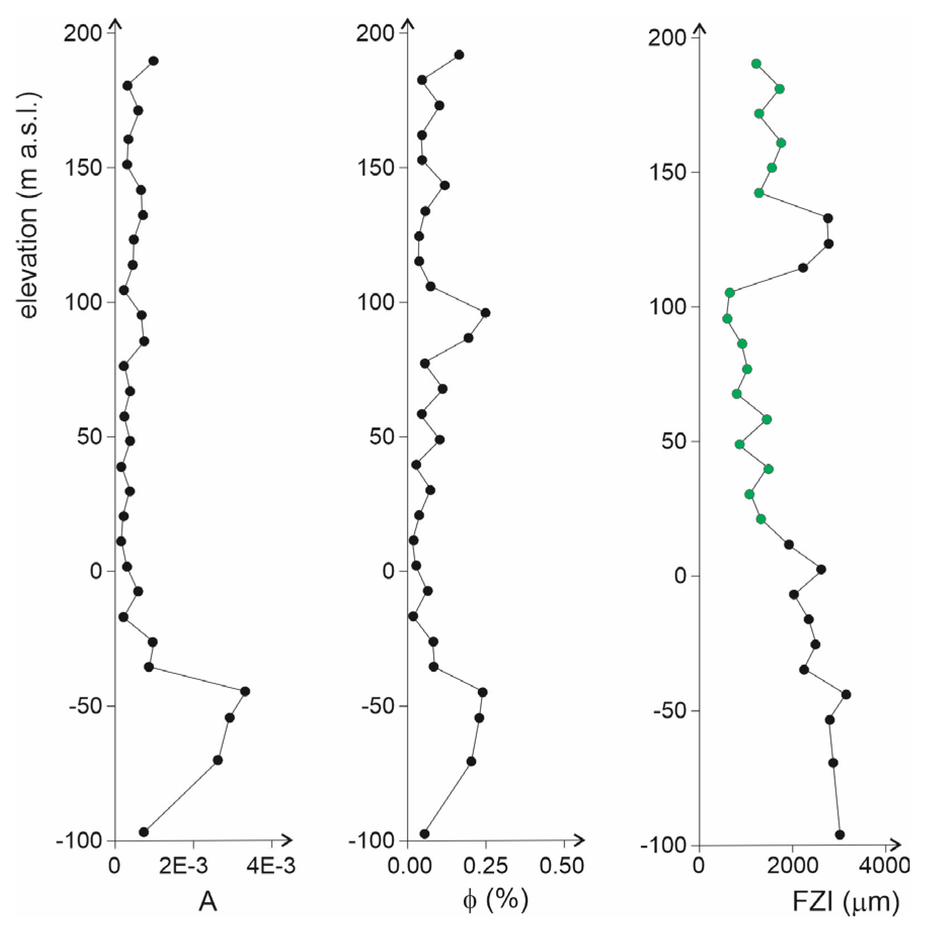
As the above computations show, aperture data vary across several orders of magnitude in all wells, likely reflecting the different intensities of post-tectonic aperture-altering processes such as cementation, dissolution, and closure. Without a detailed petrographic analysis, it is difficult to assess the relative significance of these independent effects. However, the spatial pattern along a single well (Üh-2) suggests that the combined influence of these processes defines intervals with typical behaviours (Figure 6a). In sections where A tends to increase, dissolution may be a key process, or late cementation effects are less important. Conversely, zones with unusually low A-values probably represent cemented intervals within the rock formation.
4.1. Calculated Porosities
Such differences should also lead to variations in hydrodynamic characteristics at different parts of the well. To understand the hydrodynamic behaviour of the fracture system, the fractured porosity should be calculated using the fracture model and the derived A parameter for each interval (see formulae 1–3). Based on this data, a porosity log can be created along the wells using the calibrated aperture coefficients (see Figure 6b). This porosity log differs from those estimated using an average A-value or obtained by evaluating well-log geophysical signals. It more accurately reflects the actual hydrodynamic behaviour of the rock mass and aligns more closely with measured transmissivity (permeability) data. Finally, measured permeability and calculated porosity data can be plotted on a traditional porosity-permeability cross-plot and analysed in any conventional manner (e.g., [64] and references therein; [65,66].
Figure 6.
a) Spatial pattern of the aperture coefficient (A) along the Üh-2 well indicates that the outcome of post-tectonic processes determines intervals of typical behaviours. b) A porosity log can be sketched along the well using the calibrated aperture coefficients. c) The rock body penetrated can be divided into four major zones hydrodynamically based on the FZI values.
Figure 6.
a) Spatial pattern of the aperture coefficient (A) along the Üh-2 well indicates that the outcome of post-tectonic processes determines intervals of typical behaviours. b) A porosity log can be sketched along the well using the calibrated aperture coefficients. c) The rock body penetrated can be divided into four major zones hydrodynamically based on the FZI values.
4.2. Evaluation of the Approach Introduced
Numerous methods exist to estimate how aperture varies during different WRI processes. Most experiments examine the behaviour of individual fractures. Dissolution and precipitation studies in carbonate rock samples demonstrate that, while dissolution may dominate in one part of a fracture, mineral precipitation can occur elsewhere. These small-scale variations can be measured using parameters such as the roughness coefficient [67], which are obtained through precise laboratory tests. Naturally, these results reflect the combined influence of several concurrent processes (dissolution, vein cementation) that can alter the shape of the vein wall, even within a single fracture. There are also formulae to estimate how individual fractures close with increasing depth due to lithostatic pressure [8]. Other studies aim to approximate the influence of recent stress-field anisotropy on fracture closure and/or opening [11]. However, as the angle between the principal stress axes and a fracture changes, the overall effect of stress anisotropy cannot be reliably assessed at the reservoir scale. Therefore, all these estimates of aperture change are valid on a small scale but become highly uncertain at the reservoir level, where WRI processes and pressure effects interact. Additionally, their influence can vary significantly across different points within a real rock mass. Consequently, the current approach does not attempt to understand each factor independently at a small scale. Instead, it focuses on characterising their combined effect mathematically.
In the current approach, both porosity and permeability are connected to the volume of the rock body, as measured through well hydraulics. Assuming this size is sufficiently close to the representative elementary volume (REV, [68], these hydrodynamic parameters accurately characterise the fracture system. Therefore, neither of them relates to small samples analysed under laboratory conditions.
4.3. The Case Study
On the poro-perm plot of the Üh-2 well (Figure 7), two distinct trends can be identified, both characterised by >0.9 correlation coefficients using the k = α*ϕβ regression function, where k denotes permeability, ϕ is effective porosity, and α and β are constants.
The relationship between porosity and permeability is crucial for understanding fluid flow through porous media. It is well established that higher porosity generally correlates with higher permeability. This relationship is often expressed mathematically using empirical equations, typically in the form of k = α*ϕβ, where α and β are parameters determined experimentally [69,70]. Power-law relations have also been observed across various lithologies, including sandstones and limestones [71,72]. However, it is crucial to recognise that the specific values of α and β can vary considerably depending on material properties and stress conditions [73,74]. Recent research indicates that although porosity is key to predicting permeability, effective porosity (the proportion of pore space that actively enables fluid flow) generally provides a more accurate prediction than total porosity, particularly in complex rock formations [75,76]. Furthermore, the stress field significantly influences both porosity and permeability. Under different stress conditions, pore structures within materials can change in ways that either enhance or reduce permeability [77,78]. For example, the concept of effective stress is crucial for understanding how external pressures influence the permeability-porosity relationship, particularly in shale gas reservoirs and similar geological settings [78,79]. As stress increases, it often results in pore compression, leading to decreases in both porosity and permeability [77,79].
The complexity of the relationship between porosity and permeability is also evident across various rock types. For instance, volcanic rocks show diverse permeability behaviours at different porosity levels, indicating that microstructural heterogeneity can significantly influence fluid flow paths [80,81]. Similar complexity is observed in various hard rock bodies, where fractures can significantly impact flow pathways [72,82].
In conclusion, although a direct correlation usually exists between porosity and permeability, this relationship is influenced by multiple factors, including rock type, stress conditions, and the concept of effective porosity. The importance of this relationship extends beyond theoretical models, as it holds practical significance in reservoir modelling based on measured field data.
In addition to the two trends identified in Figure 7, significantly different permeabilities are associated with the same porosity values, possibly due to varying intensities of post-deformational processes. Furthermore, segments characterised by the two distinct trends form continuous intervals along the well, suggesting that the intensities of these post-tectonic processes also vary spatially; there must be zones that are highly cemented and others mainly characterised by open fractures.
Using effective porosity and permeability data together, their variation along the well can be characterised by several parameters. Among these, the FZI (Flow Zone Indicator) is one of the most indicative of reservoir quality. Amaefule et al. [83] introduced a method to calculate the Flow Zone Indicator so that FZI = sqrt(k/ϕ)/ϕ. The lower this parameter is, the more closed the fractures are. Considering the Üh-2 well discussed above, the FZI data and trends in the poro-perm plot (Figure 7) suggest that the rock body penetrated can be divided into two main types hydrodynamically (Figure 6c). The low FZI values and the coinciding low β exponent of the fitted power function trend of the upper approximately 50 metres imply cemented fractures. This interval is followed by a 20 m short zone with high FZI values and a large β value. The coincident good reservoir quality is likely due to the presence of a hydrodynamically active fault zone. The lowermost 200 metres of the well show a continuous increase in FZI values from approximately 600 up to about 3000 μm. In this segment, the flow characteristics of the fracture system improve with depth. Whether this unusual phenomenon results from hindered vein cementation or from fractures remaining open due to the recent stress field cannot be determined without a detailed geophysical and petrological study. Nevertheless, this 200 m long interval can be divided into two sections based on the poro-perm diagram (Figure 7), indicating that a more permeable trend characterises the lower, approximately 100 m section.
The data from another nine analysed wells can be interpreted similarly. The A-parameter (aperture coefficient) generally varies by 1–2 orders of magnitude within each well, indicating significant differences in the intensities of post-tectonic processes along the wells (Figure 8). High A values clearly indicate segments with more open fractures, while low A values suggest more closed fractures.
Porosity logs further support this, showing sections with higher and lower porosity along each well (Figure 9). On poro-perm diagrams, these sections usually outline independent trends of the relation (k = α*ϕβ) between porosity and permeability (e.g., Figure 10 and Figure 11). Such trends highlight segments with similar hydrodynamic behaviours. It is important to note that in each case, data points exhibiting similar hydrodynamic behaviour are not randomly distributed across the wells; instead, they appear side by side and define specific depth intervals. In these intervals, the effectiveness of petrological and/or structural processes that influenced the aperture must have been characteristic. These sections can be described as hydraulic flow units (HFU; [83,84], which are best identified along the wells using their FZI logs [85] (Figure 12).
The relationship between the Flow Zone Indicator (FZI) values and Hydraulic Flow Units (HFUs) in fractured rock masses is a key concept in reservoir geology. The FZI characterises rock properties related to fluid flow, which is essential for understanding and predicting reservoir performance. HFUs are defined as volumes of rock where the geological and petrophysical properties that influence fluid movement are internally consistent [86]. This uniformity is crucial because it determines how fluid interacts with the rock matrix. As the FZI is a composite index that combines the rock’s porosity and permeability, it offers insight into the flow characteristics within a given HFU. The FZI value reflects the hydraulic properties of the rock; for example, a higher FZI value generally indicates better reservoir quality and higher permeability, thereby improving fluid flow potential.
Research has shown that different rock types and geological conditions influence FZI values and, consequently, the classification of HFUs within fractured rock masses [36,86]. Several studies demonstrate the applicability of FZI in predicting HFUs. For example, [87] found that incorporating FZI calculations significantly improved the identification of HFUs in the Bredasdorp Basin, indicating that consistent FZI values reflect similar hydraulic flow characteristics [87,88]. Likewise, [89] emphasised the usefulness of FZI in enhancing the accuracy of permeability predictions based on rock typing in carbonate formations.
Considering all calculated data, the FZI values of the Mórágy granite are very high compared with those typical of intergranular-porosity reservoirs (mainly sandstones). However, they fall within the common range for other fractured rock masses, such as carbonates [90,91]. Nonetheless, the specific FZI values are inconsistent, varying by two orders of magnitude across the studied wells, with an FZI of approximately 40 μm for Üh-4. In contrast, the lowermost part of the Üh-22 well reaches a maximum of 4000 μm.
Based on the typical vertical pattern with well-defined sections of markedly different FZI values, all studied wells can be divided into numerous HFUs. In the case of Üh-3 (Figure 12a), FZI~500 m is consistent throughout the well, with two zones of unusually low FZI values. The sudden appearance of these zones indicates the presence of fault zones hosting highly mineralised veins. All porosity and permeability data follow the same pattern for Üh-4 (Figure 10), suggesting a similar post-tectonic evolution of the fracture system around it. Low FZI values are consistent throughout the crosscut segment, indicating uniform hydraulic behaviour of the surrounding rock mass. In the case of the Üh-5 well, three distinct trends can be identified in the poro-perm plot (Figure 11). Samples belonging to each of these groups represent well-defined depth intervals along the well, with FZ indicator values decreasing steadily downward (Figure 12c). Such behaviour reflects fracture closure with increasing depth, due to rising lithostatic pressure or enhanced significance for vein mineralisation.
In the fracture system of the Üh-22 well, the measured permeabilities vary across a range of four orders of magnitude (Table 1, Figure 13a). Simultaneously, the estimated porosities range between 0.05% and 1.2% (Figure 13b). The coinciding poro-perm plot (Figure 14) indicates three distinct trends, all of which correspond to separate depth intervals (HFUs). A continuously decreasing FZI trend is characteristic of the well (Figure 13 c), reaching its minimum at approximately -50 m (a.s.l.), where very low aperture coefficients (~5E-4) are typical, likely due to intensive vein mineralisation. Further down, the sharply increasing FZI values (from ~300 μm to ~3000 μm) denote a new hydraulic flow unit at the lowest studied interval. This pattern is not evident on either the permeability or porosity logs (Figure 13a, b), but it reliably correlates with the observed hydrodynamic behaviour of the well. Comparing the FZI log with the hydraulic head profile of the same well [58] Figure 13d) reveals an apparent coincidence: near-uniform head values extend down to about -140 m (a.s.l.), followed by an abrupt drop in head at the bottom 70 m of the well, where anomalously open fractures in the new HFU can be inferred. This pattern supports the model proposed by [61], which suggests that the lowermost section of the well is isolated from the upper part by an intensively altered and mutually fractured horizon, rather than by a sparse fracture network. Benedek et al. [92] also emphasise that the compartmentalised behaviour of the granitoid reservoir often results from extensive secondary mineralisation of specific fracture zones.
The Üh-25 (Figure 12d) well exhibits behaviour similar to that of Üh-3. Its profile, characterised by a typical FZI value, is interrupted by a roughly 20 m wide zone of low values. This zone can likely be interpreted as a highly mineralised fault zone. The behaviour of Üh-26 (Figure 12e) resembles that of Üh-2 and Üh-22, with a nearly constant FZI trend that decreases downward and two zones of higher values, indicating high-permeability fault zones. An apparent bimodality is evident in the case of Üh-27 (Figure 12f). High FZI values dominate the upper part of the well, whereas lower values are typical as the well extends downwards. Given that the well penetrates the granitoid massif at the boundary between two lithologically distinct realms (Figure 3), the vertical pattern appears to reflect these lithological and rheological changes.
A previous evaluation [35] showed that the two lithologies could be characterised by significantly different fracture network parameters (D, E) and connectivity relationships. Consequently, the hydrodynamic behaviour of the fracture network in the monzogranite and monzonite-dominated blocks should also differ. Along with the Üh-28 well (Figure 12g), a continuous decrease in FZI values is typical, with no sudden change, suggesting that the well probably did not intersect any major fault zone. However, the data define two HFUs, as the values reach a threshold at approximately 100 m (a.s.l.), and the data follow a different trend in the poro-perm plot (Figure 15). The FZI pattern exhibited by Üh-29 (Figure 12h) is similar to those of Üh-2, Üh-22, and Üh-26. A consistent decreasing FZI trend is observed throughout the entire well, with two roughly 20 m wide intervals where the values jump abruptly. The very high FZI values in these intervals suggest hydraulically active fault zones at these depths.
Considering all studied wells, the fractured Mórágy granite can be characterised by the simultaneous presence of numerous hydraulic flow units, with their boundaries identifiable using FZI logs in each case. Most wells penetrating the granitoid body exhibit homogeneous or slightly decreasing FZI values downwards, interrupted by sections sometimes 10 m wide, where an abrupt change in FZI values is typical. These anomalous zones also define independent trends on the poro-perm plot. While the continuous decline in FZI may reflect fracture closure due to increasing lithostatic pressure, the jumps along the logs indicate discontinuous changes. In the case of Üh-27, such variation in FZI values can be interpreted as resulting from two alternating granitoid lithologies. Nevertheless, all other cases likely indicate the presence of a fault zone. In agreement with previous structural geological and hydrogeological studies [58], some fault zones in the area are highly mineralised and behave as impermeable barriers, while others serve as efficient groundwater conduits. The vertical profiles shown by Üh-2, -22, -26, and -29 align well with the widely accepted hydrodynamic model of the region, in which less-transmissive blocks (fractured rock bodies) coexist with more-transmissive zones (fault zones). Conversely, the vertical patterns of Üh-3 and -25 exemplify the presence of intensely mineralised fault zones.
A more detailed analysis of the aperture, effective porosity, and FZI logs of all studied wells is beyond the scope of this paper, as it would require a more specific geological background. The limited examples provided, however, demonstrate the applicability of the introduced algorithm for estimating the aperture coefficient, fractured porosity, and the Flow Zone Indicator by simultaneously using measured transmissivity data and DFN models.
5. Conclusions
Overall, the approach described above offers many advantages. Calculating reliable hydraulic aperture coefficients from fracture geometry data and measured transmissivities provides crucial insights into how fractures open and close in the studied wells. The fracture aperture values can then be utilised to determine the effective fractured porosity, which specifically focuses on the hydrodynamic behaviour of that particular segment of the rock formation and can be assessed alongside permeabilities in a consistent manner. By fitting power function curves on the standard poro-perm diagram, fractured intervals with similar fracture closure characteristics can be identified. Effective porosity and permeability values derived from the same dataset and related to the same rock body can also be used to calculate other important indices, such as the FZI mentioned above. The analysis of data from ten wells penetrating the fractured Mórágy granitoid in SW Hungary demonstrates that, based on the estimated hydrodynamic behaviour of individual intervals, hydraulic flow units with distinct characteristics can be distinguished in each well.
One of the main challenges in studying fractured reservoirs is extending porosity and permeability data to unexplored areas of the rock formation. Although a detailed discussion of this issue is beyond the scope of the present paper, having reliable fracture aperture coefficients for individual wells enables interpolation of aperture data between wells. Using actual hydraulic aperture data may provide a practical method for estimating viable porosity and permeability fields.
Funding
This research was funded by the National Research, Development and Innovation Office (Grant No. K-138919).
Acknowledgments
Gy. Dankó is acknowledged for providing the transmissivity data measured in the evaluated wells.
Conflicts of Interest
The author declares no conflicts of interest.
Abbreviations
The following abbreviations are used in this manuscript:
| DFN | discrete fracture network |
| L | fracture length |
| N(L) | number of fractures of length L |
| E | length exponent |
| F | constant in the fracture length distribution function |
| N(r) | number of boxes in the box counting algorithm |
| D | fractal dimension of fracture midpoints |
| α | dip of a fracture |
| β | dip angle of a fracture |
| a | aperture |
| A | aperture coefficient |
| Φ | porosity |
| v | specific flow rate |
| μ | dynamic viscosity |
| ρ | fluid density |
| J | hydraulic gradient |
| K | hydraulic conductivity |
| T | transmissivity |
| d | thickness of the saturated interval |
| k | permeability |
References
- Tsakiroglou, C.D.; Klint, K.E.S.; Nilsson, B.; Theodoropoulou, M.A.; Aggelopoulos, C.A. From aperture characterisation to hydraulic properties of fractures. Geoderma 2012, 181–182, 65–77. [Google Scholar] [CrossRef]
- Caulk, R. A.; Ghazanfari, E.; Perdrial, J. N.; Perdrial, N. Experimental investigation of fracture aperture and permeability change within Enhanced Geothermal Systems. Geothermics 2016, 62, 12–21. [Google Scholar] [CrossRef]
- Vidal, J.; Genter, A.; Chopin, F. Permeable fracture zones in the hard rocks of the geothermal reservoir at Rittershoffen, France. J. Geophys. Res. Solid Earth 2017, 122, 4864–4887. [Google Scholar] [CrossRef]
- Nelson, R. A. Geologic Analysis of Naturally Fractured Reservoirs, 2nd ed.; Gulf Professional Publishing, 2001. [Google Scholar]
- Twiss, R. J.; Moores, E. Structural geology; W H Freeman, 1992; p. 532. [Google Scholar]
- Blaisonneau, A.; Peter-Borie, M.; Gentier, S. Evolution of fracture permeability with respect to fluid/rock interactions under thermohydromechanical conditions: development of experimental reactive percolation tests. Geotherm. Energy 2016, 4/3. [Google Scholar] [CrossRef]
- Ceccato, A.; Viola, G.; Tartaglia, G.; Antonellini, M. In-situ quantification of mechanical and permeability properties on outcrop analogues of offshore fractured and weathered crystalline basement: Examples from the Rolvsnes granodiorite, Bømlo, Norway. Mar. Pet. Geol. 2021, 124, 104859. [Google Scholar] [CrossRef]
- Morrow, C.; Lockner, D.; Hickman, S.; Rusanov, M.; Röckel, T. Effects of lithology and depth on the permeability of core samples from the Kola and KTB drill holes. J. Geophys. Res. 1994, 99/B4, 7263–7274. [Google Scholar] [CrossRef]
- Allen, T. O.; Roberts, A. P. Production Operations; Oil and Gas Consultants International, Inc.: Tulsa, 1982; pp. 113–169. [Google Scholar]
- Bisdom, K.; Bertotti, G.; Nick, H. M. The impact of in-situ stress and outcrop-based fracture geometry on hydraulic aperture and upscaled permeability in fractured reservoirs. Tectonophysics 2016, 690, 63–75. [Google Scholar] [CrossRef]
- Becker, I.; Müller, B.; Koehrer, B.; Jelinek, W.; Hilgers, C. Present-day stress control on fluid migration pathways: Case study of the Zechstein fractured carbonates, NW-Germany. Mar. Pet. Geol. 2019, 103, 320–330. [Google Scholar] [CrossRef]
- Gudmundsson, A.; Kusumoto, S.; Simmenes, T. H.; Philipp, S. L.; Larsen, B.; Lotveit, I. F. Effects of overpressure variations on fracture apertures and fluid transport. Tectonophysics 2012, 581, 220–230. [Google Scholar] [CrossRef]
- Kaufmann, G.; Gabrovšek, F.; Romanov, D. Dissolution and precipitation of fractures in soluble rock. Hydrol. Earth Syst. Sci. Discuss. 2016. [Google Scholar] [CrossRef]
- Germanovich, L.N.; Astakhov, D.K. Fracture closure in extension and mechanical interaction of parallel joints. J. Geophys. Res. 2004. [Google Scholar] [CrossRef]
- Kumar, S.; Bodvarsson, G. S. Fractal study and simulation of fracture roughness. Geophys. Res. Lett. 1990, 17, 701–704. [Google Scholar] [CrossRef]
- 16. Liu, E. (2005): Effects of fracture aperture and roughness on hydraulic and mechanical properties of rocks: implication of seismic characterisation of fractured reservoirs. J. Geophys. Eng. 2/1, 38–47. [CrossRef]
- Brabazon, J. W.; Perfect, E.; Gates, C. H.; Santodonato, L. J.; Dhiman, I.; Bilheux, H.; Bilheux, J. C.; McKay, L. D. Spontaneous Imbibition of a Wetting Fluid Into a Fracture With Opposing Fractal Surfaces: Theory and Experimental Validation. Fractals 2019. [Google Scholar] [CrossRef]
- Ni, X.; Niu, Y.; Wang, Y. Non-Darcy Flow Experiments of Water Seepage through Rough-Walled Rock Fractures. Geofluids 2018. [Google Scholar] [CrossRef]
- Wang, C.; Jiang, Y.; Luan, H.; Sugimoto, S. Effect of shearing on hydraulic properties of rough-walled fractures under different boundary conditions. Energy Sci. Eng. 2019. [Google Scholar] [CrossRef]
- Li, M.; Liu, X.; Li, Y.; Hou, Z.; Quiao, S. Effect of Contact Areas on Seepage Behavior in Rough Fractures under Normal Stress. Int. J. Geomech. 2021, 22/4. [Google Scholar] [CrossRef]
- Stock, B.; Frampton, A. Fracture aperture generation using surface scan measurements of natural rock samples. In ESS Open Archive; 2023. [Google Scholar] [CrossRef] [PubMed]
- Bauer, M.; M. Tóth, T. Characterisation and DFN modelling of the fracture network in a Mesozoic karst reservoir: Gomba oilfield, Paleogene Basin, Central Hungary. J. Pet. Geol. 2017, 40/3, 319–334. [Google Scholar] [CrossRef]
- Cheng, C.; Hale, S.; Milsch, H.; Blum, P. Measuring hydraulic fracture apertures: a comparison of methods. In Solid Earth; 2020. [Google Scholar] [CrossRef]
- Ye, Z.; Liu, H. H.; Jiang, Q.; Zhou, C. Two-phase flow properties of a horizontal fracture: The effect of aperture distribution. Adv. Water Resour. 2015, 76, 43–54. [Google Scholar] [CrossRef]
- Ramandi, H. L.; Armstrong, R. T.; Mostaghimi, P. Micro-CT image calibration to improve fracture aperture measurement. Case Stud. Nondestruct. Test. Eval. 2016, 6, 4–13. [Google Scholar] [CrossRef]
- Laubach, S. E.; Baumgardner, R. W., Jr.; Monson, E. R.; Hunt, E.; Meador, K. J. Fracture Detection in Low-Permeability Reservoir Sandstone: A Comparison of BHTV and FMS Logs to Core. SPE Pap. 1988, no. 18119. [Google Scholar]
- Cao, Y.B.; Feng, X.T.; Yan, E. C.; Chen, G.; Lü, F. F.; Ji, H. B.; Song, K. Y. Calculation Method and Distribution Characteristics of Fracture Hydraulic Aperture from Field Experiments in Fractured Granite Area. Rock. Mech. Rock. Eng. 2015. [Google Scholar] [CrossRef]
- Leckenby, R. J.; Sanderson, D. J.; Lonergan, L. Estimating flow heterogeneity in natural fracture systems. J. Volcanol. Geotherm. Res. 2005, 148/1–2, 116–129. [Google Scholar] [CrossRef]
- Nordqvist, A. W.; Tsang, Y. W.; Tsang, C. F.; Verstorp, B.; Andersson, J. A Variable Aperture Fracture Network Model for Flow and Transport in Fractured Rocks. Water Resour. Res. 1992, 28/6, 1703–1713. [Google Scholar] [CrossRef]
- Sun, J. P.; Zhao, Z. Y. Influences of Fracture Aperture and Roughness on Hydraulic Conductivity in Fractured Rock Mass. Recent progresses in fluid dynamics research. Proceeding Sixth Int. Conf. Fluid Mech. AIP Conf. Proc. 2011, Vol., 406–408. [Google Scholar]
- Tóth, T.M.; Vass, I. Relationship Between the Geometric Parameters of Rock Fractures, the Size of Percolation Clusters and REV. Math. Geosci. 2011, 43/1, 75–97. [Google Scholar]
- Dershowitz, W. S.; Einstein, H. H. Characterising rock joint geometry with joint system models. Rock. Mech. Rock. Eng. 1988, 21, 21–51. [Google Scholar] [CrossRef]
- Hewett, T. A. Fractal Methods for Fracture Characterization. In Stochastic Modeling and Geostatistics. Principles, Methods and Case Studies. AAPG Computer Applications in Geology, 3.; Yarus, J. M., Chambers, R. L., Eds.; AAPG: Tulsa, 1995. [Google Scholar]
- Long, J. C. S. (Ed.) Rock fractures and fluid flow: contemporary understanding and applications; National Academy Press: Washington D. C., 1996; p. 551. [Google Scholar]
- M. Tóth, T. Fracture network characterisation using 1D and 2D data of the Mórágy Granite body, Southern Hungary. J. Struct. Geol. 2018, 113, 176–187. [Google Scholar] [CrossRef]
- Tóth, E.; Hrabovszki, E.; Schubert, F.; M. Tóth, T. Discrete fracture network (DFN) modelling of a high-level radioactive waste repository host rock and the effects on its hydrogeological behaviour. J. Struct. Geol. 2022a, 156, 104556. [Google Scholar] [CrossRef]
- Tóth, E.; Hrabovszki, E.; Schubert, F.; M. Tóth, T. Lithology-controlled hydrodynamic behaviour of a fractured sandstone-claystone body in a radioactive waste repository site, SW Hungary. Appl. Sci. 2022b, 12/5, 2528. [Google Scholar]
- Bonnet, E.; Bour, O.; Odling, N. E.; Davy, P.; Main, I.; Cowie, P.; Berkowitz, B. Scaling of fracture systems in geological media. Rev. Geophys. 2001, 39/3, 347–383. [Google Scholar] [CrossRef]
- Tóth, T.M.; Hollós, Cs.; Szűcs, É.; Schubert, F. Conceptual fracture network model of the crystalline basement of the Szeghalom Dome (Pannonian Basin, SE Hungary). Acta Geol. Hung. 2004, 47/1, 19–34. [Google Scholar] [CrossRef]
- Graf, T.; Therrien, R. A method to discretize non-planar fractures for 3D subsurface flow and transport simulations. Numer. Methods Fluids 2007. [Google Scholar] [CrossRef]
- Yang, S.; Wang, M.; Zheng, S.; Zeng, S.; Gao, L. Fractal Permeability Model of Newtonian Fluids in Rough Fractured Dual Porous Media. Materials 2022. [Google Scholar] [CrossRef] [PubMed]
- Bour, O.; Davy, P. Connectivity of random fault networks following a power law fault length distribution. Water Resour. Res. 1997, 33, 1567–1583. [Google Scholar] [CrossRef]
- Barton, C. C.; Larsen, E. Fractal geometry of two-dimensional fracture networks at Yucca Mountain, Southwestern Nevada. In Proc. Int. Symp. on Fundamentals of Rock Joints; Stephanson, O., Ed.; 1985; pp. 77–84. [Google Scholar]
- La Pointe, P. R. A method to characterise fracture density and connectivity through fractal geometry. Int. J. Rock. Mech. Min. Sci. Geomech. Abstr. 1988, 25, 421–429. [Google Scholar] [CrossRef]
- M. Tóth, T. Determination of geometric parameters of fracture networks using 1D data. J. Struct. Geol. 2010, 32, 878–885. [Google Scholar] [CrossRef]
- Vermilye, J. M.; Scholz, C. H. Relation between vein length and aperture. J. Struct. Geol. 1995, 17/3, 423–434. [Google Scholar] [CrossRef]
- Gudmundsson, A. Fracture dimensions, displacements and fluid transport. J. Struct. Geol. 2000, 22/9, 1221–1231. [Google Scholar] [CrossRef]
- Gudmundsson, A.; Berg, S. S.; Lyslo, K. B.; Skurtveit, E. Fracture networks and fluid transport in active fault zones. J. Struct. Geol. 2001, 23/2-3, 343–353. [Google Scholar] [CrossRef]
- Olson, J. E. Sublinear scaling of fracture aperture versus length: an exception or the rule? J. Geophys. Res. 2003, 108, 2413. [Google Scholar] [CrossRef]
- Oda, M. Permeability tensor for discontinuous rock masses. Geotechnique 1985, 35, 483–495. [Google Scholar] [CrossRef]
- Witherspoon, P. A.; Wang, J. S. Y.; Iwai, K.; Gale, J. E. Validity of cubic law for fluid flow in deformable rock fracture. Water Resour. Res. 1980, 16/6, 1016–1024. [Google Scholar] [CrossRef]
- Neuzil, C. E.; Tracy, J. V. Flow through fractures. Water Resour. Res. 1981, 17/1, 191–199. [Google Scholar] [CrossRef]
- Koike, K.; Ichikawa, Y. Spatial correlation structures of fracture systems for deriving a scaling law and modeling fracture distributions. Comput. Geosci. 2006, 32/8, 1079–1095. [Google Scholar] [CrossRef]
- Aguilera, R.; Houston, M.; Podia, A. L.; Song, S. J. SPE 17545; Well Test Analysis of Pumping Wells in Multiphase Naturally Fractured Reservoirs. 1988.
- Stewart, G.; Ascharsobbi, F. Well Test Interpretation for Naturally Fractured Reservoirs. SPE Paper, 1988; no. 18173. [Google Scholar]
- Király, E.; Koroknai, B. The magmatic and metamorphic evolution of the north-eastern part of the Mórágy Block. Annual Report of the Geological Institute of Hungary 2003, 2004; pp. 299–300. [Google Scholar]
- Rotár-Szalkai, Á.; Eper-Pápai, I.; Mentes, Gy. Well level data analysis in Hungary near a fault region. J. Geodyn. 2006, 41, 183–189. [Google Scholar] [CrossRef]
- Benedek, K.; Dankó, Gy. Stochastic hydrogeological modelling of fractured rocks: a generic case study in the Mórágy Granite Formation (South Hungary). Geol. Carpathica 2009, 60(4), 271–281. [Google Scholar] [CrossRef]
- Benedek, K.; Molnár, P. Combining structural and hydrogeological data: Conceptualisation of a fracture system. Eng. Geol. 2013, 163, 1–10. [Google Scholar] [CrossRef]
- Maros, Gy.; Koroknai, B.; Palotás, K.; Fodor, L.; Dudko, A.; Forián-Szabó, M.; Zilahi-Sebess, L.; Bán-Győry, E. Tectonic analysis and structural evolution of the north-eastern Mórágy Block. Annual Report of the Geological Institute of Hungary 2003, 2004; pp. 370–386. [Google Scholar]
- Balla, Z.; Horváth, I.; Tóth, Gy.; Benedek, K.; Mező, Gy.; Molnár, P. Hydrogeological pattern of the Bátaapáti (Üveghuta) site. Annual Report of the Geological Institute of Hungary 2003, 2004; pp. 449–472. [Google Scholar]
- Maros, Gy.; Palotás, K. Evaluation of planar features in boreholes Üh–22 and Üh–23 near Üveghuta with CoreDump software. Annual Report of the Geological Institute of Hungary 1999, 2000; pp. 315–339. [Google Scholar]
- Zilahi-Sebess, L.; Mészáros, F.; Szongoth, G. Characterisation of fracture zones in granite, based on well-logging data at the Üveghuta site. Annual Report of the Geological Institute of Hungary 2002, 2003; pp. 253–266. [Google Scholar]
- Xu, P.; Yu, B. Developing a new form of permeability and Kozeny–Carman constant for homogeneous porous media by means of fractal geometry. Adv. Water Resour. 2008, 31, 74–81. [Google Scholar] [CrossRef]
- Grude, S.; Dvorkin, J.; Landrø, M. Permeability variation with porosity, pore space geometry, and cement type: A case history from the Snøhvit field, the Barents Sea. Geophysics 2015, 80/1, 43–49. [Google Scholar]
- Dernaika, M.; Masalmeh, S.; Mansour, B.; Al Jallad, O.; Koronfol, S. Geology-Based Porosity-Permeability Correlations in Carbonate Rock Types. SPE Pap. 2019, no. 196665. [Google Scholar]
- Scalco, L.; Tonietto, L.; Velloso, R.Q.; Racolte, G.; Veronez, M. R. Determination of roughness coefficient in 3D digital representations of rocks. Sci. Rep. 2022, 12(1), 10822. [Google Scholar] [CrossRef] [PubMed]
- Bear, J. Dynamics of fluids in porous media; Elsevier: Amsterdam, 1972; p. 784. [Google Scholar]
- Le, B.; Vu, T.; Nguyen, H.; Hưng, V. A genetic programming-assisted analytical formula for predicting the permeability of pervious concrete. Eng. Technol. Appl. Sci. Res. 2024, 14(3), 14775–14780. [Google Scholar] [CrossRef]
- Chen, S.; Dong, X.; Chen, Y.; Dong, Z.; Zhao, B.; Jiang, L.; Chen, Z. Characterization of the porosity and permeability of gasified coal in ucg process: an experimental and simulation study. ACS Omega 2025, 10(1), 1308–1319. [Google Scholar] [CrossRef] [PubMed]
- Meng, F.; Baud, P.; Ge, H.; Wong, T. The effect of stress on limestone permeability and effective stress behavior of damaged samples. J. Geophys. Res. Solid Earth 2019, 124(1), 376–399. [Google Scholar] [CrossRef]
- Heap, M.; Bayramov, K.; Meyer, G.; Violay, M.; Reuschlé, T.; Baud, P.; Gilg, H. A.; Harnett, C. E.; Kushnir, A. R. L.; Lazari, F.; Mortensen, A. K. Compaction and permeability evolution of tuffs from krafla volcano (Iceland). J. Geophys. Res. Solid Earth 2024, 129(8). [Google Scholar] [CrossRef]
- Bernabé, Y.; Mok, U.; Evans, B. Permeability-porosity relationships in rocks subjected to various evolution processes. Pure Appl. Geophys. 2003, 160(5-6), 937–960. [Google Scholar] [CrossRef]
- Al-Khdheeawi, E.; Allawi, R.; Al-Rubaye, W.; Iglauer, S. A new approach to predicting vertical permeability for carbonate rocks in the southern mesopotamian basin. Minerals 2023, 13(12), 1519. [Google Scholar] [CrossRef]
- Li, Y.; Wang, W.; Haonan, L.; He, J.; Zhang, X.; Wu, Y. Prediction of permeability coefficient of complex graded non-cohesive soil. Res. Sq. 2023. [Google Scholar] [CrossRef] [PubMed]
- Wang, H. Analysis of the permeability capacity and engineering performance of porous asphalt concrete. Materials 2025, 18(17), 4200. [Google Scholar] [CrossRef] [PubMed]
- Zhang, Y.; Xu, X.; Lebedev, M.; Sarmadivaleh, M.; Barifcani, A.; Iglauer, S. Multi-scale x-ray computed tomography analysis of coal microstructure and permeability changes as a function of effective stress. Int. J. Coal Geol. 2016, 165, 149–156. [Google Scholar] [CrossRef]
- Reyes, L.; Osisanya, S. Empirical correlation of effective stress dependent shale rock properties. J. Can. Pet. Technol. 2000, 41(12). [Google Scholar] [CrossRef]
- Belhaj, H.; Vaziri, H.; Islam, M. Laboratory investigation of effective stresses’ influence on petrophysical properties of sandstone reservoirs during depletion. J. Can. Pet. Technol. 2009, 48(07), 47–53. [Google Scholar] [CrossRef]
- Wadsworth, F.; Vasseur, J.; Scheu, B.; Kendrick, J.; Lavallée, Y.; Dingwell, D. Universal scaling of fluid permeability during volcanic welding and sediment diagenesis. Geology 2016, 44(3), 219–222. [Google Scholar] [CrossRef]
- Heap, M.; Meyer, G.; Noël, C.; Wadsworth, F.; Baud, P.; Violay, M. The permeability of porous volcanic rock through the brittle-ductile transition. J. Geophys. Res. Solid Earth 2022, 127(6). [Google Scholar] [CrossRef] [PubMed]
- Peng, R.; Di, B.; Glover, P.; Wei, J.; Lorinczi, P.; Ding, P.; Liu, Z.; Yuangui, Z.; Wu, M. The effect of rock permeability and porosity on seismoelectric conversion: experiment and analytical modelling. Geophys. J. Int. 2019, 219(1), 328–345. [Google Scholar] [CrossRef]
- Amaefule, J. O.; Altunbay, M.; Tiab, D.; Kersey, D. G.; Keeland, D. K. SPE Paper no. 26436; Enhanced reservoir description: using core and log data to identify hydraulic (flow) units and predict permeability in uncored intervals/wells. 1993.
- Hearn, C.L.; Ebanks, W.J., Jr.; Tye, R.S.; Ranganathan, V. Geological Factors Influencing Reservoir Performance of the Hartzog Draw Field, Wyoming. J. Pet. Technol. 1984, 36, 1335–1344. [Google Scholar] [CrossRef]
- Orodu, O. D.; Tang, Z.; Fei, Q. Hydraulic (Flow) Unit Determination and Permeability Prediction: a Case Study of Block Shen-95, Liaohe Oilfield, Nort-East China. J. Appl. Sci. 2009, 9/10, 1801–1816. [Google Scholar] [CrossRef]
- Ha, M. Q.; Le, A. N.; Jarzyna, J. Hydraulic flow unit classification from core data: case study of the Z gas reservoir, Poland. J. Min. Earth Sci. 2021, 62(3), 29–36. [Google Scholar] [CrossRef]
- Opuwari, M.; Afolayan, B.; Mohammed, S.; Amaechi, P.; Bareja, Y.; Chatterjee, T. Petrophysical core-based zonation of ow oilfield in the bredasdorp basin south africa. Sci. Rep. 2022, 12(1). [Google Scholar] [CrossRef] [PubMed]
- Opuwari, M.; Mohammed, S.; Ile, C. Determination of reservoir flow units from core data: a case study of the lower cretaceous sandstone reservoirs, western bredasdorp basin offshore in South Africa. Nat. Resour. Res. 2020, 30(1), 411–430. [Google Scholar] [CrossRef]
- Zhang, Z.; Cai, Z. Permeability prediction of carbonate rocks based on digital image analysis and rock typing using random forest algorithm. Energy Fuels 2021, 35(14), 11271–11284. [Google Scholar] [CrossRef]
- Soto, B. R.; Arteaga, D.; Martin, C.; Rodriguez, F. Pore-Type Determination From Core Data Using a New Polar-Transformation Function from Hydraulic Flow Units. SPE Pap. 2010, no, 136805. [Google Scholar]
- Kosari, E.; Kadkhodaie, A.; Bahroudi, A.; Chehrazi, A.; Talebian, M. An integrated approach to study the impact of fractures distribution on the Ilam-Sarvak carbonate reservoirs: A case study from the Strait of Hormuz, the Persian Gulf. J. Pet. Sci. Eng. 2017, 152, 104–115. [Google Scholar] [CrossRef]
- Benedek, K.; Bőthi, Z.; Mező, Gy.; Molnár, P. Compartmented flow at the Bátaapáti site in Hungary. Hydrogeol. J. 2009, 17, 1219–1232. [Google Scholar] [CrossRef]
Figure 1.
The volume of the fractures is estimated using Riemann’s approximation algorithm. Here, increasing the value of n improves the accuracy of the estimate.
Figure 1.
The volume of the fractures is estimated using Riemann’s approximation algorithm. Here, increasing the value of n improves the accuracy of the estimate.
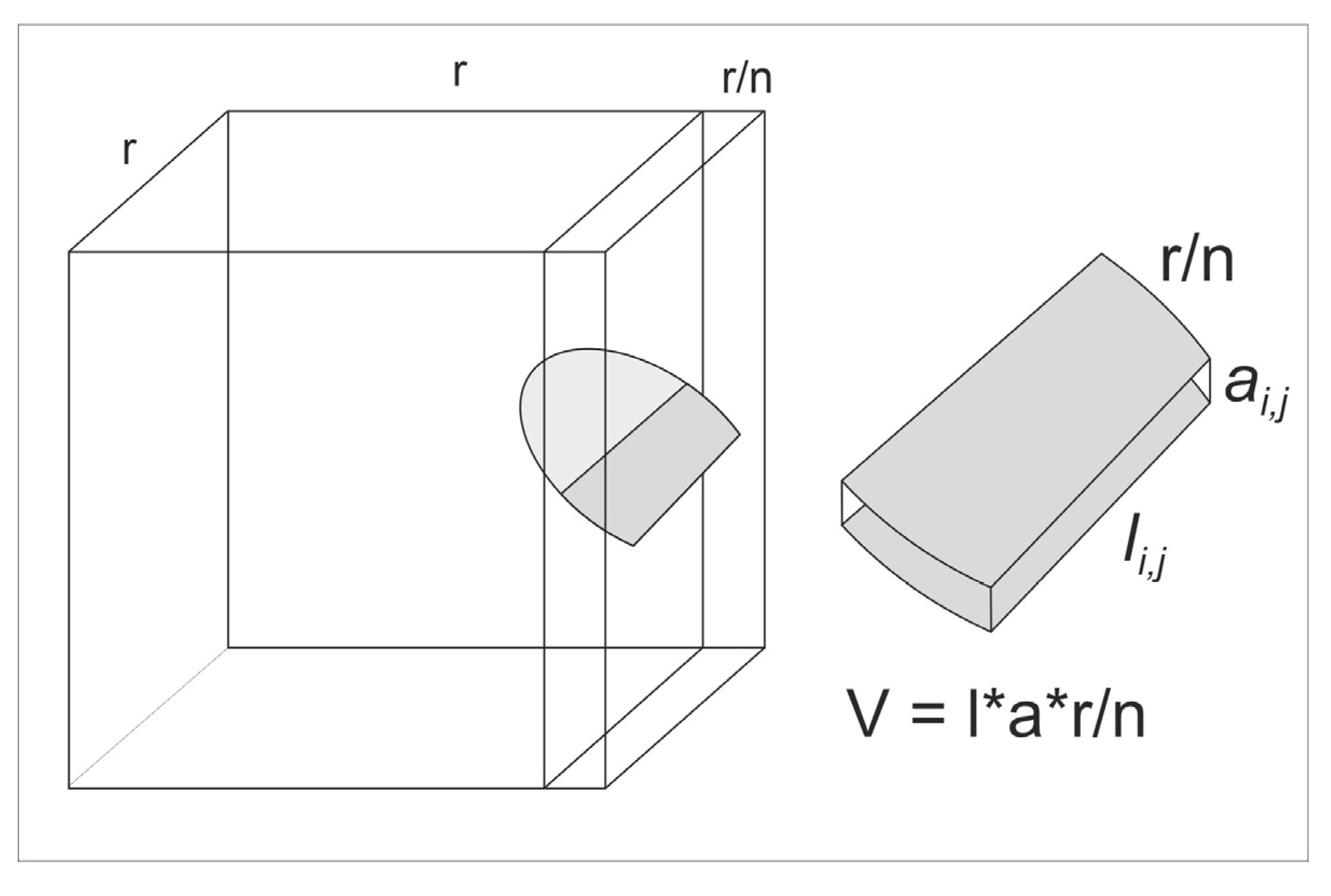
Figure 2.
The logical diagram of the algorithm for calibrating the fracture aperture coefficient. In the final stage, permeability values obtained from the pumping test (observed) are compared with those calculated using a DFN model of the same rock segment (estimated). For further details, refer to the text.
Figure 2.
The logical diagram of the algorithm for calibrating the fracture aperture coefficient. In the final stage, permeability values obtained from the pumping test (observed) are compared with those calculated using a DFN model of the same rock segment (estimated). For further details, refer to the text.
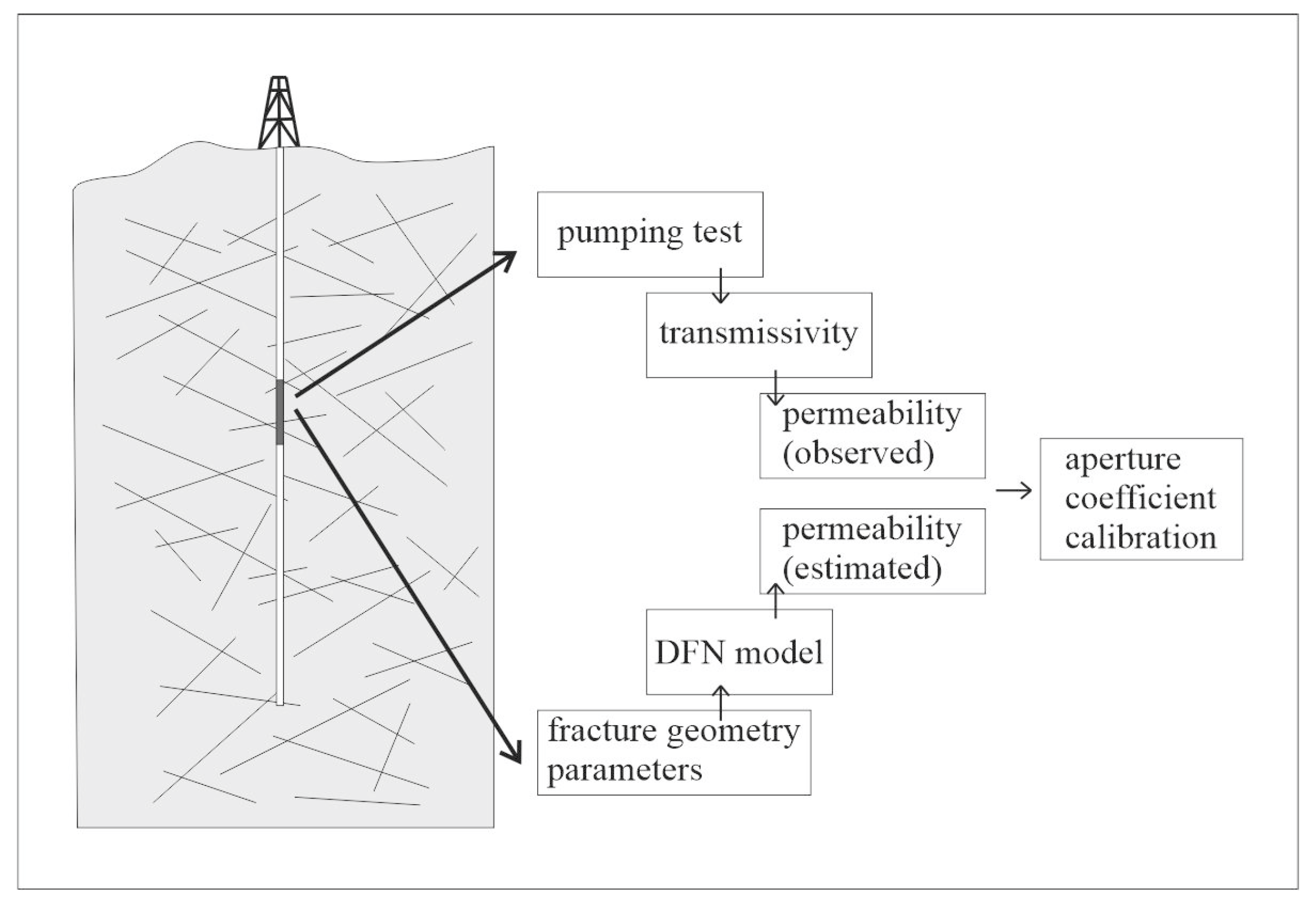
Figure 3.
The location of the Mórágy Granite Formation (MGF) in SW Hungary. a) Geological sketch map of the study area with the positions of the studied boreholes (red dots). The black lines indicate significant fault zones. The two varieties of granitoid rocks are coloured, with pink representing monzogranite and green representing the monzonite-dominated region.
Figure 3.
The location of the Mórágy Granite Formation (MGF) in SW Hungary. a) Geological sketch map of the study area with the positions of the studied boreholes (red dots). The black lines indicate significant fault zones. The two varieties of granitoid rocks are coloured, with pink representing monzogranite and green representing the monzonite-dominated region.
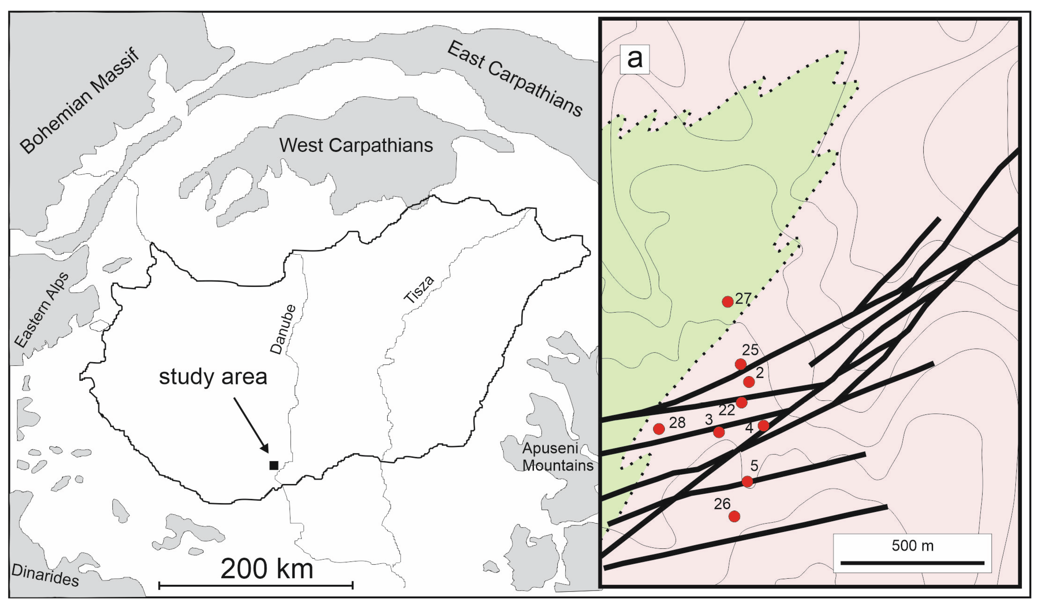
Figure 4.
The calculated D values and the final fracture network model for well Üh-2.
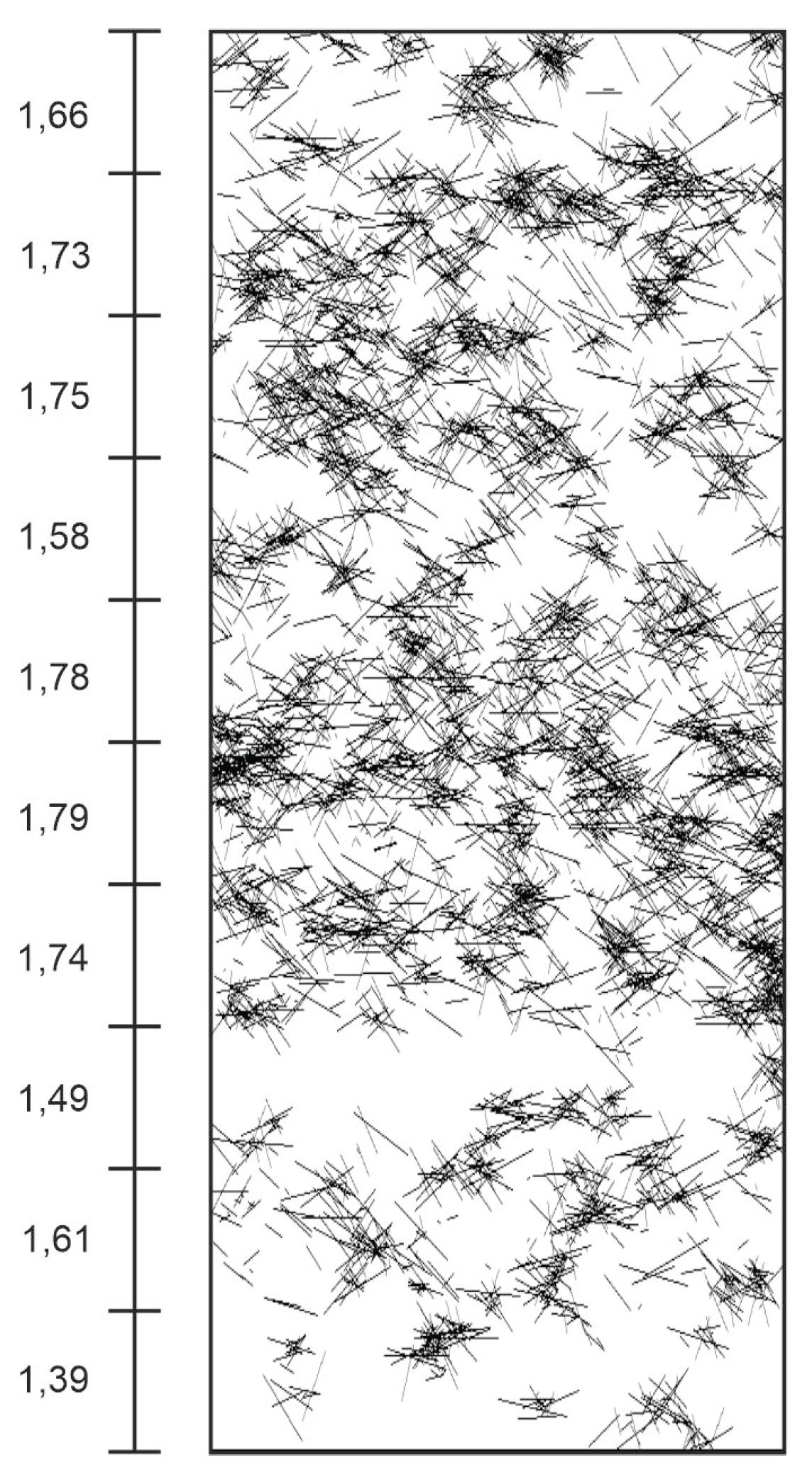
Figure 5.
By fitting a logarithmic curve to the points on the A versus log(kobs)/log(kest) plot, the A value (aperture coefficient) can be identified where log(kobs)/log(kest) equals 1. The black dots represent simulated data used for calibration, while the grey dot indicates the calibrated A value.
Figure 5.
By fitting a logarithmic curve to the points on the A versus log(kobs)/log(kest) plot, the A value (aperture coefficient) can be identified where log(kobs)/log(kest) equals 1. The black dots represent simulated data used for calibration, while the grey dot indicates the calibrated A value.
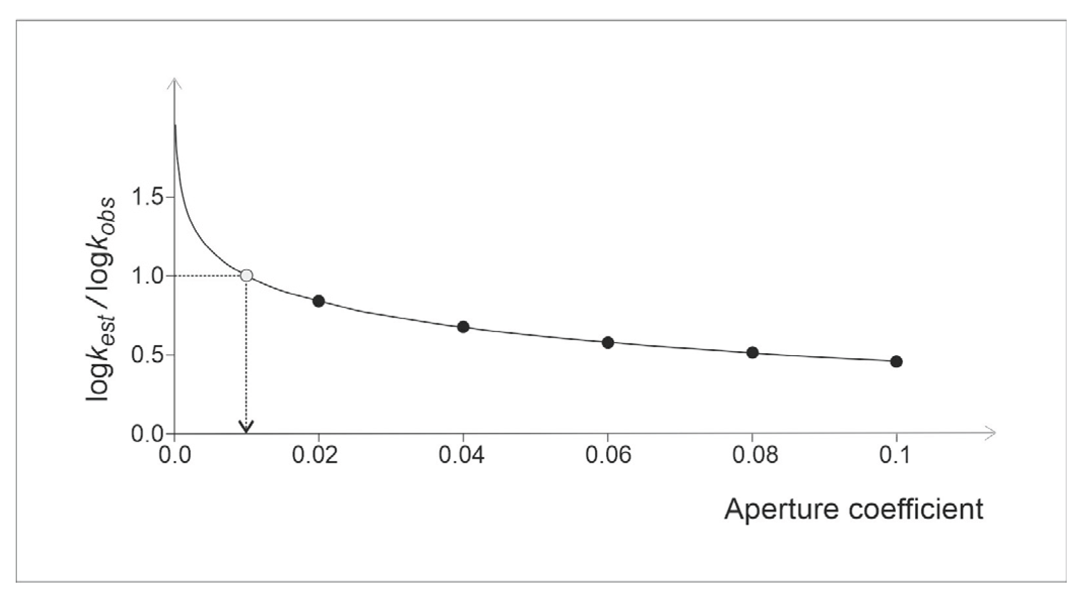
Figure 7.
The poro-perm diagram of the Üh-2 well displays measured permeability and estimated effective porosity data plotted. The data points show two best-fit trends, indicating two different hydrodynamic behaviours (compare with the intervals shown by the green and black dots along the well in Figure 6c).
Figure 7.
The poro-perm diagram of the Üh-2 well displays measured permeability and estimated effective porosity data plotted. The data points show two best-fit trends, indicating two different hydrodynamic behaviours (compare with the intervals shown by the green and black dots along the well in Figure 6c).
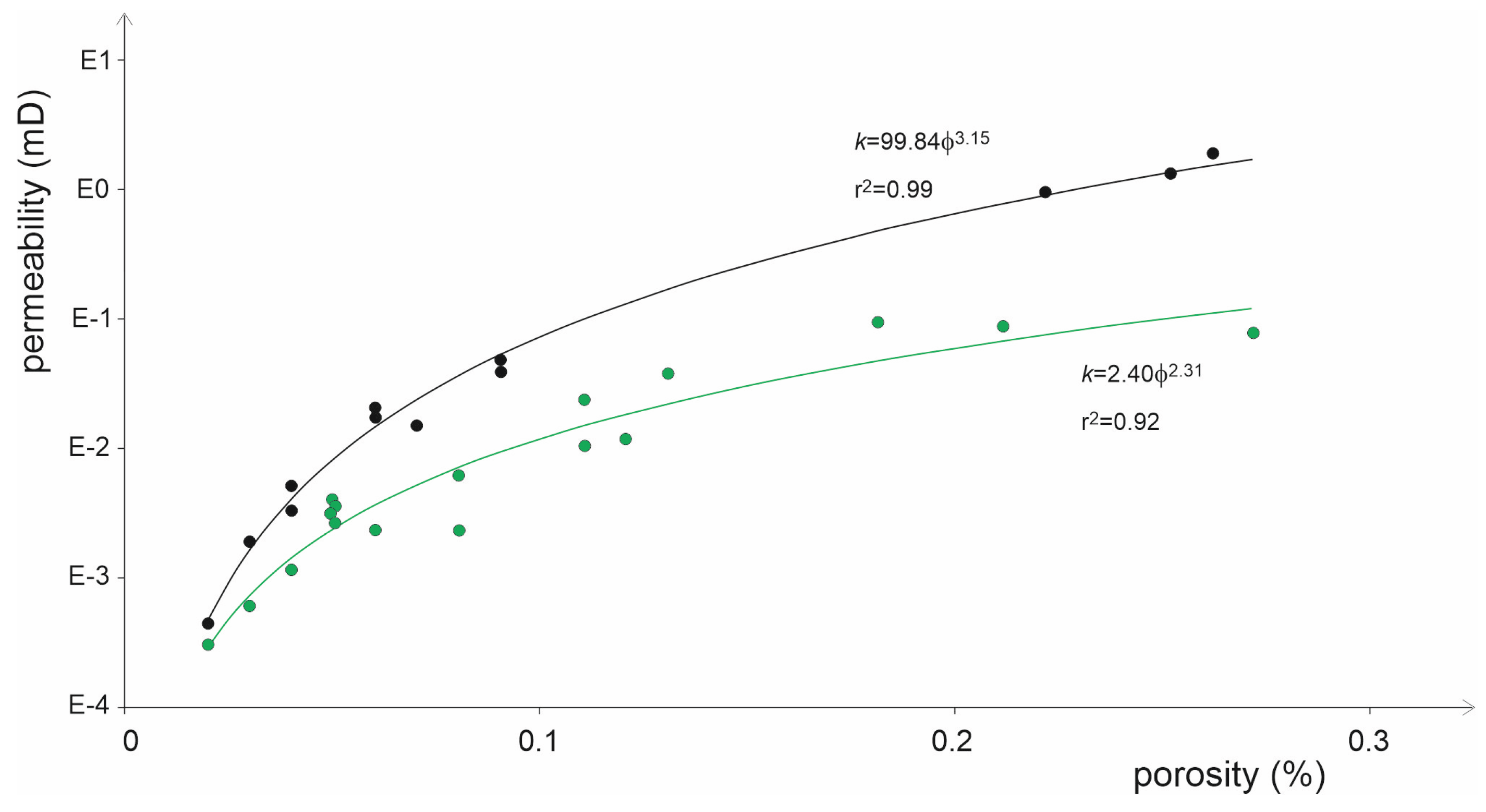
Figure 8.
The A parameter typically varies over 1–2 orders of magnitude, indicating that the intensities of post-tectonic processes fluctuate across all studied wells. a) Üh-3 well, b) Üh-4 well, c) Üh-5 well, d) Üh-25 well, e) Üh-26 well, f) Üh-27 well, g) Üh-28 well, h) Üh-29 well.
Figure 8.
The A parameter typically varies over 1–2 orders of magnitude, indicating that the intensities of post-tectonic processes fluctuate across all studied wells. a) Üh-3 well, b) Üh-4 well, c) Üh-5 well, d) Üh-25 well, e) Üh-26 well, f) Üh-27 well, g) Üh-28 well, h) Üh-29 well.
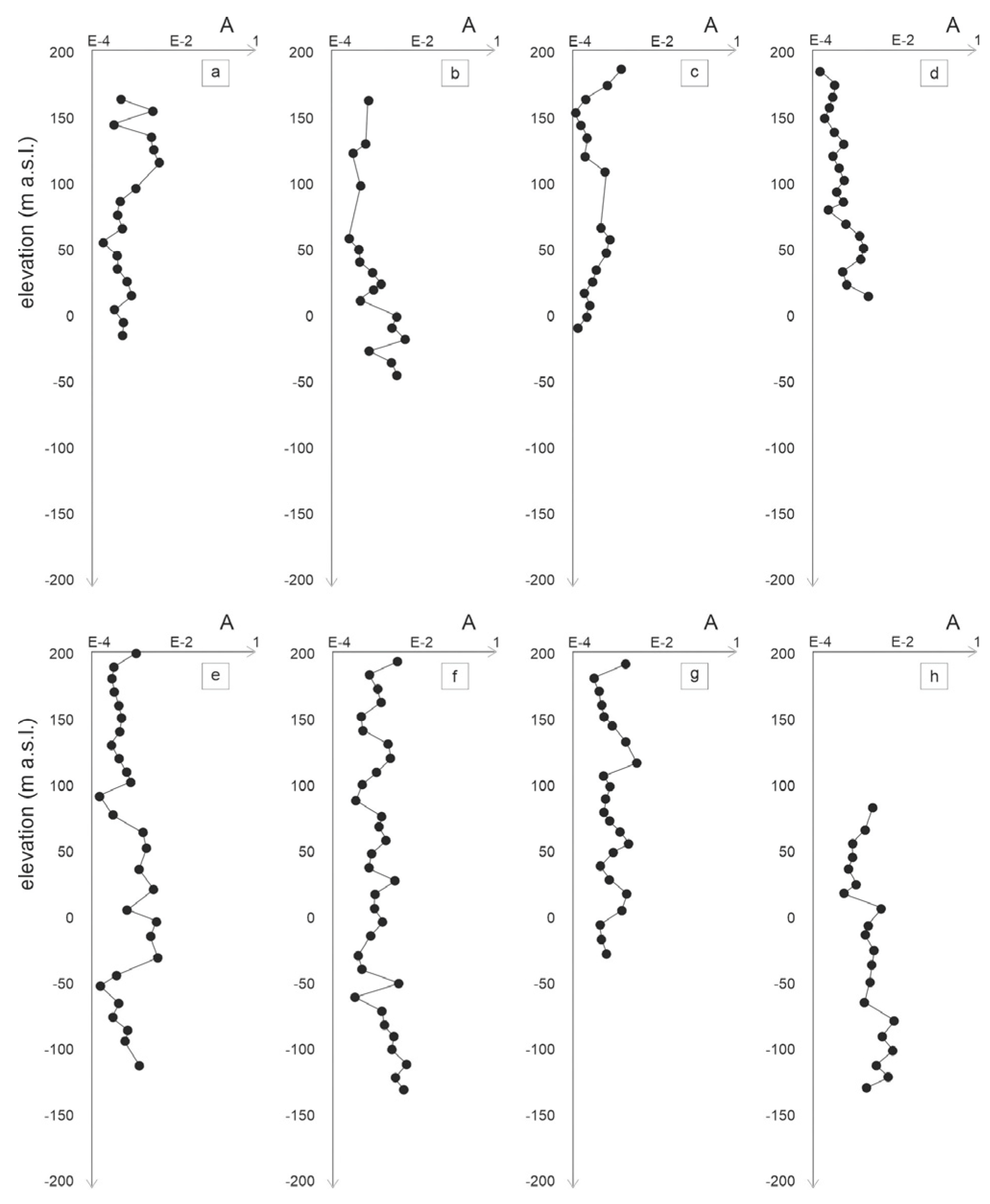
Figure 9.
The calculated porosity logs of the studied wells. a) Üh-3 well, b) Üh-4 well, c) Üh-5 well, d) Üh-25 well, e) Üh-26 well, f) Üh-27 well, g) Üh-28 well, h) Üh-29 well.
Figure 9.
The calculated porosity logs of the studied wells. a) Üh-3 well, b) Üh-4 well, c) Üh-5 well, d) Üh-25 well, e) Üh-26 well, f) Üh-27 well, g) Üh-28 well, h) Üh-29 well.
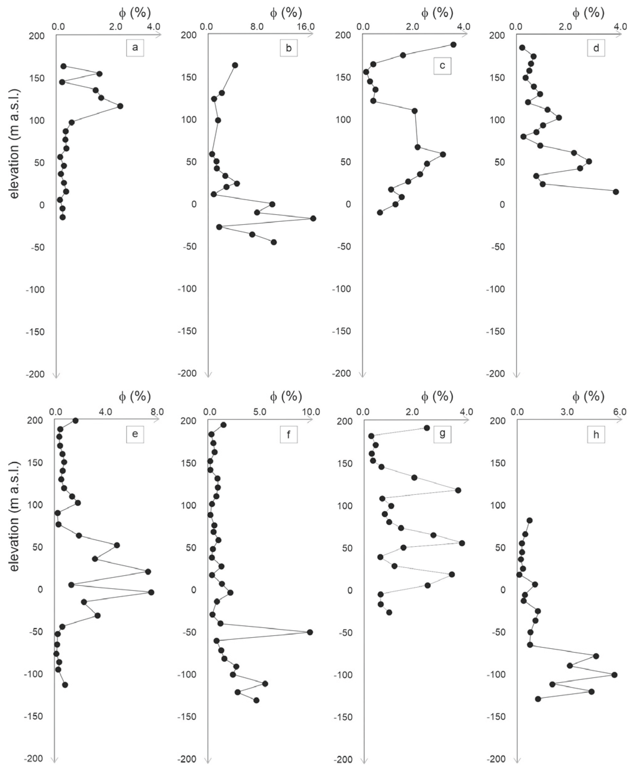
Figure 10.
All data points follow the same trend on the poro-perm plot of the Üh-4 well.
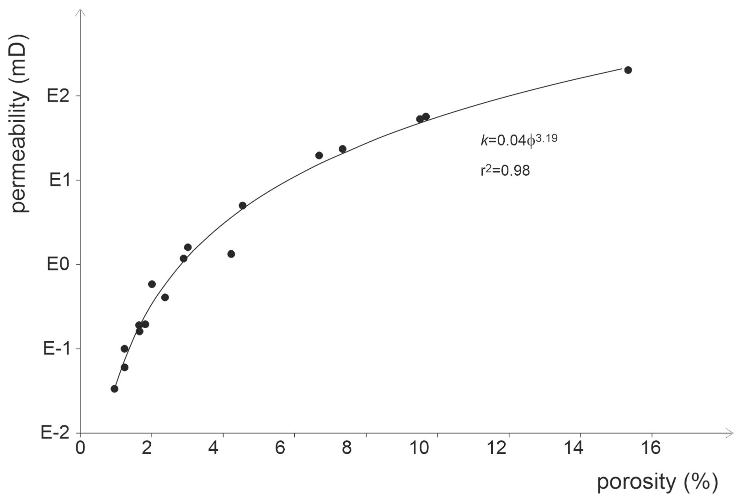
Figure 11.
For the Üh-5 well, three distinct best-fit trends are identifiable in the poro-perm plot.
Figure 11.
For the Üh-5 well, three distinct best-fit trends are identifiable in the poro-perm plot.
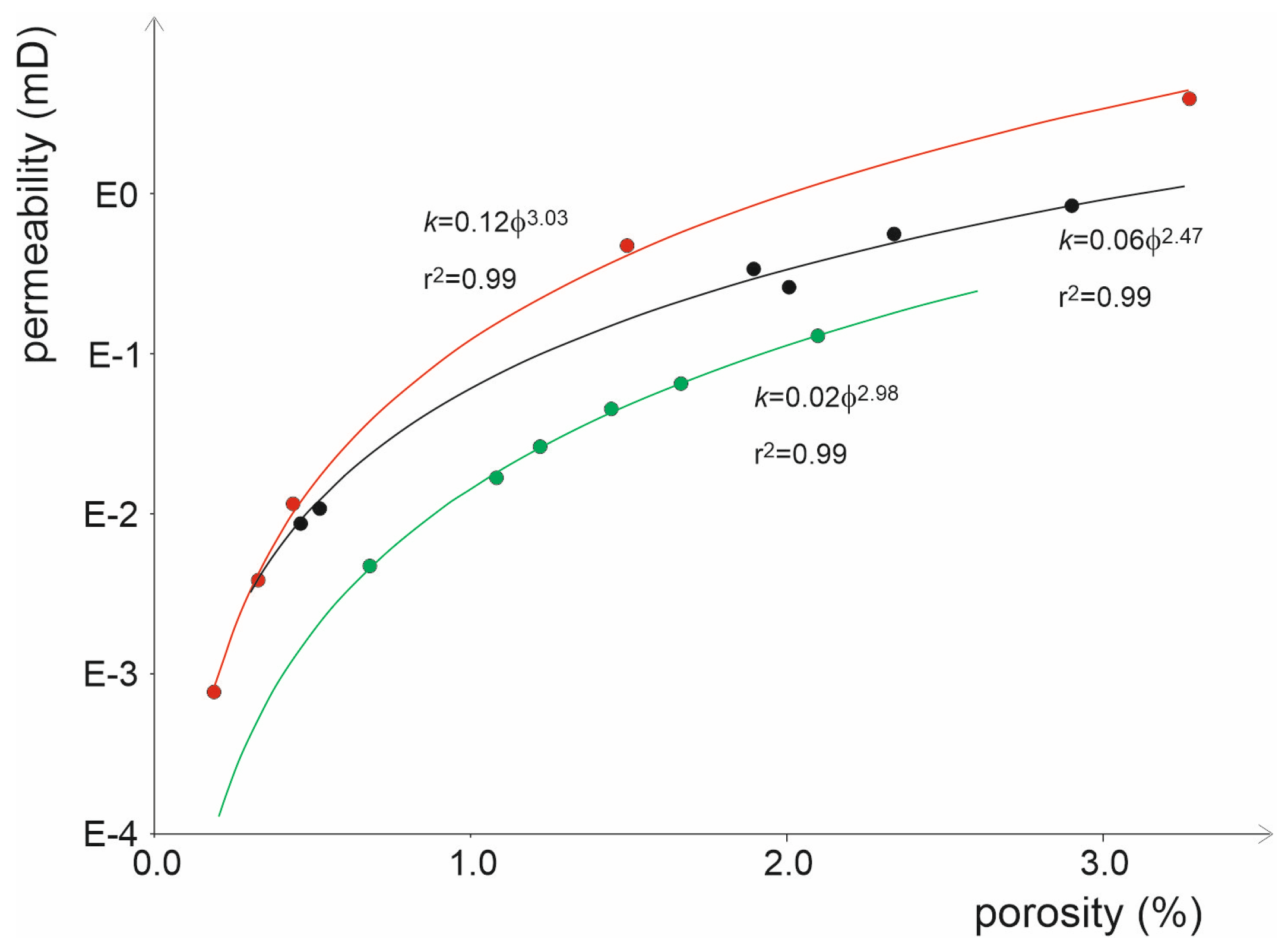
Figure 12.
The calculated Flow Zone Indicator (FZI in μm) logs display segments with different hydrodynamic behaviours (hydraulic flow units) across all wells. Data points in various colours represent different trends on the poro-perm diagrams. a) Üh-3 well, b) Üh-4 well, c) Üh-5 well, d) Üh-25 well, e) Üh-26 well, f) Üh-27 well, g) Üh-28 well, h) Üh-29 well.
Figure 12.
The calculated Flow Zone Indicator (FZI in μm) logs display segments with different hydrodynamic behaviours (hydraulic flow units) across all wells. Data points in various colours represent different trends on the poro-perm diagrams. a) Üh-3 well, b) Üh-4 well, c) Üh-5 well, d) Üh-25 well, e) Üh-26 well, f) Üh-27 well, g) Üh-28 well, h) Üh-29 well.
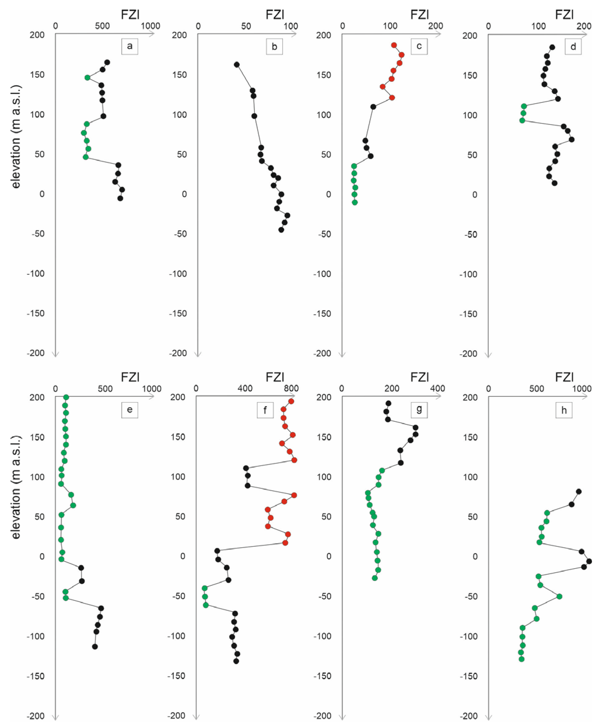
Figure 13.
Typical hydrodynamic logs of the Üh-22 well. a) Measured permeability log, b) porosity log based on the estimated aperture coefficient (A), c) FZI log calculated using measured permeability and estimated porosity data, d) the hydraulic head profile of the well [58].
Figure 13.
Typical hydrodynamic logs of the Üh-22 well. a) Measured permeability log, b) porosity log based on the estimated aperture coefficient (A), c) FZI log calculated using measured permeability and estimated porosity data, d) the hydraulic head profile of the well [58].
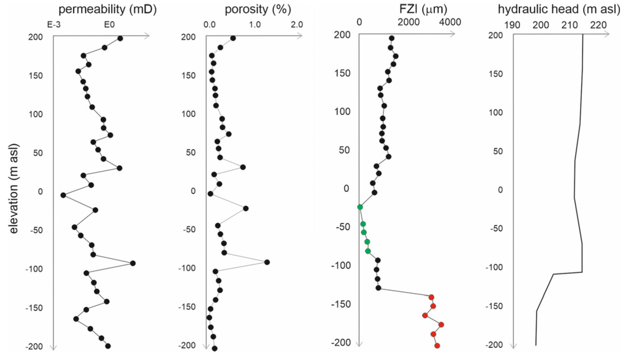
Figure 14.
Three distinct best-fit trends characterise the fracture system of the Üh-22 well on the poro-perm diagram.
Figure 14.
Three distinct best-fit trends characterise the fracture system of the Üh-22 well on the poro-perm diagram.
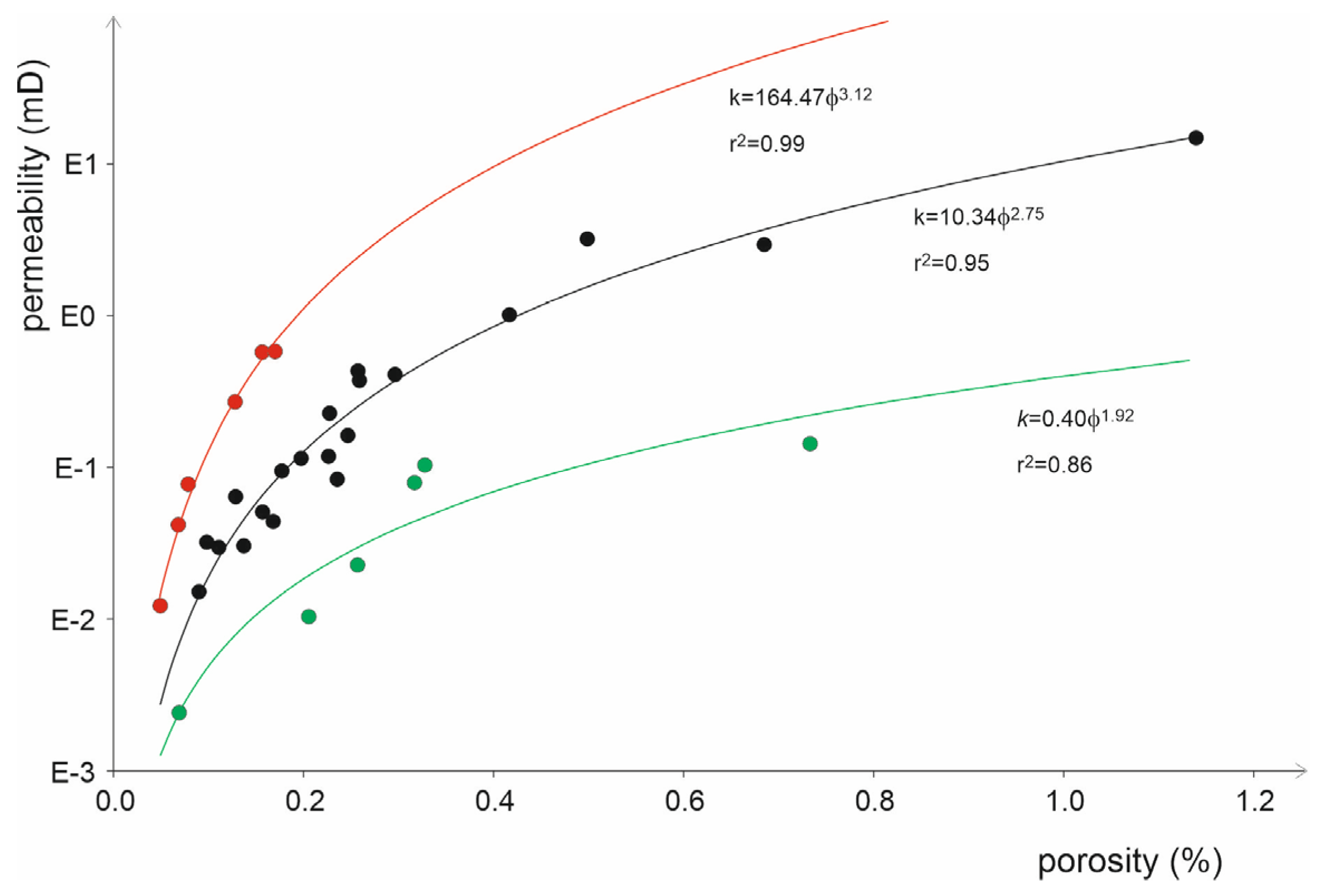
Figure 15.
The poro-perm plot of well Üh-28.
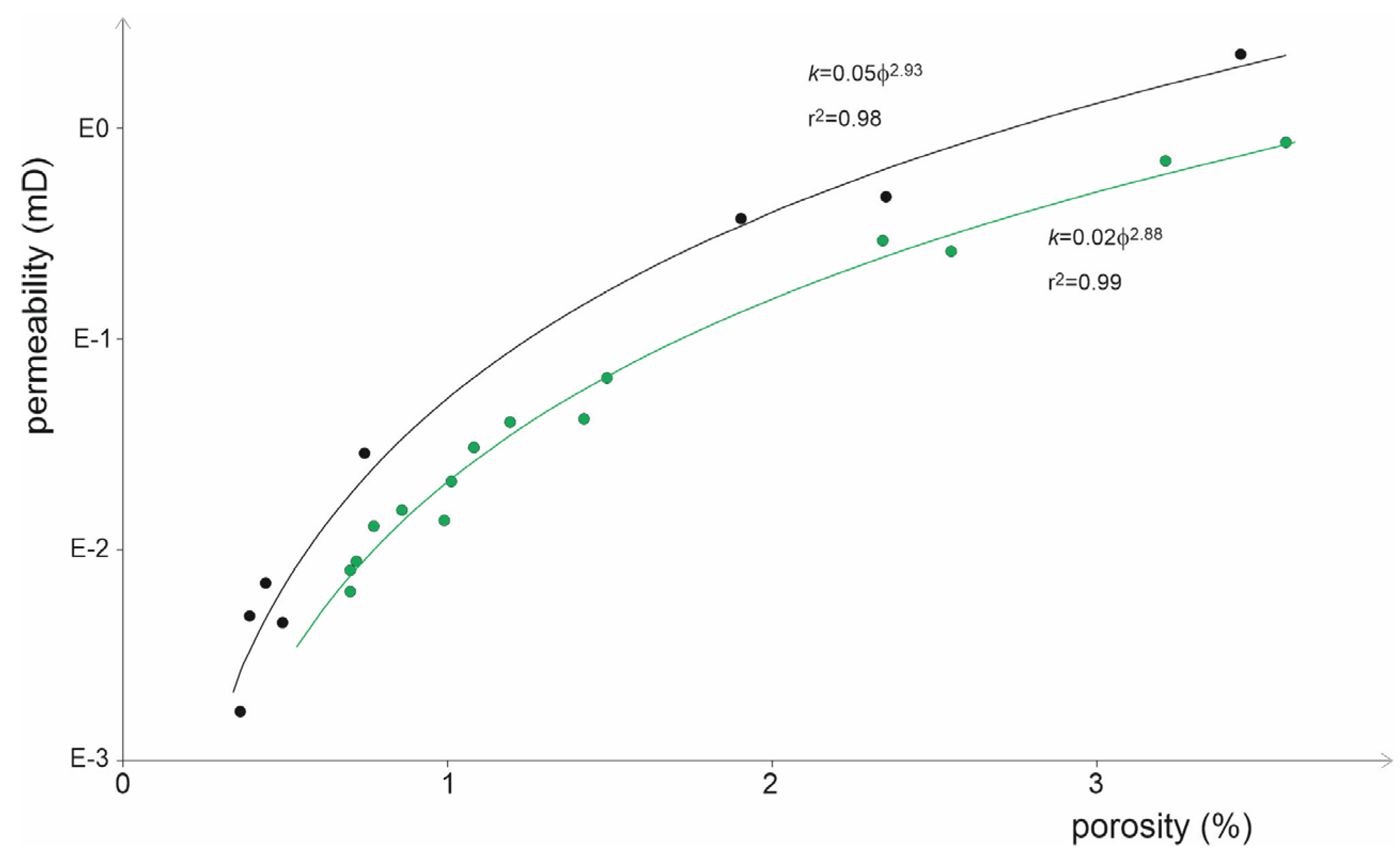

Table 1.
Basic statistical parameters (minimum, maximum, and mean) of permeabilities (in m2) in the studied wells calculated from measured transmissivities. Averages are harmonic means.
Table 1.
Basic statistical parameters (minimum, maximum, and mean) of permeabilities (in m2) in the studied wells calculated from measured transmissivities. Averages are harmonic means.
| well | # | kmin | kmax | kavg | well | # | kmin | kmax | kavg |
|---|---|---|---|---|---|---|---|---|---|
| Üh-2 | 29 | 3.0E-18 | 1.8E-14 | 2.4E-17 | Üh-25 | 20 | 3.8E-17 | 7.8E-14 | 2.7E-16 |
| Üh-3 | 18 | 2.0E-17 | 2.4E-13 | 1.6E-16 | Üh-26 | 28 | 2.6E-17 | 4.1E-13 | 2.5E-16 |
| Üh-4 | 17 | 3.4E-16 | 2.2E-12 | 2.2E-15 | Üh-27 | 32 | 1.3E-16 | 1.0E-12 | 1.1E-15 |
| Üh-5 | 17 | 7.8E-18 | 3.9E-14 | 7.7E-17 | Üh-28 | 23 | 1.7E-16 | 2.3E-13 | 1.2E-15 |
| Üh-22 | 34 | 2.4E-17 | 1.5E-13 | 3.3E-16 | Üh-29 | 20 | 2.1E-16 | 1.8E-12 | 2.0E-15 |
Disclaimer/Publisher’s Note: The statements, opinions and data contained in all publications are solely those of the individual author(s) and contributor(s) and not of MDPI and/or the editor(s). MDPI and/or the editor(s) disclaim responsibility for any injury to people or property resulting from any ideas, methods, instructions or products referred to in the content. |
© 2026 by the authors. Licensee MDPI, Basel, Switzerland. This article is an open access article distributed under the terms and conditions of the Creative Commons Attribution (CC BY) license (http://creativecommons.org/licenses/by/4.0/).
Copyright: This open access article is published under a Creative Commons CC BY 4.0 license, which permit the free download, distribution, and reuse, provided that the author and preprint are cited in any reuse.


