
Submitted:
17 July 2026
Posted:
17 July 2026
You are already at the latest version
Abstract
Autonomous driving technology imposes stringent requirements on real-time environmental perception and dynamic distance measurement, which are critical prerequisites for vehicle path planning and driving safety. Traditional ranging methods relying on LiDAR and visual sensors often suffer from poor real-time performance and insufficient robustness in complex and dynamic traffic scenarios. To address this limitation, this paper proposes a novel fixed-time zeroing neural network (ZNN) to achieve high-precision and real-time inter-vehicle distance estimation for autonomous vehicles. First, a time-varying optimization model for inter-vehicle distance calculation is established based on dynamic programming theory, which fully considers the motion trajectories and structural constraints of adjacent vehicles. Subsequently, a dedicated activation function is designed to construct the improved fixed-time ZNN model for solving the above time-varying optimization problem. Rigorous theoretical proofs are presented to verify the fixed-time stability of the proposed network, and a tight upper bound of the convergence time is analytically derived. Moreover, comprehensive parameter selection strategies are discussed to guide practical model deployment. Finally, numerical simulation results demonstrate that the developed ZNN model possesses faster convergence speed and stronger robustness compared with existing methods, and it can accurately complete real-time distance calculation within a fixed time upper bound. The proposed method provides a new effective solution for dynamic ranging tasks in autonomous driving systems.
Keywords:
autonomous driving
; inter-vehicle real-time distance estimation
; fixed-time stability
; ZNN
; activation function
; time-varying optimization
MSC: 34D20,90C30, 90C31, 65L20
1. Introduction
The rapid advancement of autonomous driving has raised rigorous demands for vehicles’ environmental perception and decision-making capabilities. As a core perception task, real-time inter-vehicle distance measurement directly determines the reliability of path planning and driving safety for intelligent vehicles. Although LiDAR, visual sensors and other traditional techniques can acquire distance information, their real-time responsiveness and anti-interference ability are greatly restricted in dynamic traffic environments. In recent years, zeroing neural networks (ZNNs) have exhibited unique advantages in real-time optimization and dynamic system control due to their inherent fixed-time convergence property.
Different from conventional neural networks optimized by cost functions, ZNNs are constructed based on error dynamics. Their fundamental principle is to drive the system state to converge to an equilibrium point by designing specific error functions. By utilizing error derivative information to dynamically adjust network parameters, ZNNs realize real-time state tracking without relying on iterative operations, thus guaranteeing superior real-time performance. In general, ZNNs have three prominent merits: strong adaptability to real-time systems, low sensitivity to initial values with high robustness, and powerful capability to handle nonlinear and time-varying problems. Since first proposed by Zhang Yunong in [1], ZNNs have become a popular research direction and been widely applied in robot trajectory tracking [2,3,4], matrix inversion [5,6,7], time-varying quadratic programming [8,9,10] and other fields. Nevertheless, research on applying ZNNs to autonomous driving ranging tasks remains scarce. In this paper, a new fixed-time ZNN will be given to solve the problem of autonomous driving.
Fixed-time stability is a special form of finite-time stability which refers to the ability of a system to converge to an equilibrium point in finite time and regardless of the initial value chosen, the convergence time is not greater than a fixed upper bound. Therefore, fixed-time stability has stronger robustness and is widely used. The concept of fixed-time stability was first proposed by Polyakovin [11], who also established the corresponding stability criteria and derived the convergence time upper bound. Exploring new stability criteria and obtaining tighter convergence time limits have long been the key challenges in this research field. Several effective criteria and time upper bounds have been reported in previous studies [12,13], including our earlier works [7,14], which also discussed parameter selection rules and parameter sensitivity analysis in [7] and [14].
Inspired by the existing theoretical frameworks, this paper develops a new fixed-time ZNN model for the real-time distance estimation problem in autonomous driving. The fixed-time stability of the proposed model is strictly proven, and the corresponding convergence time upper bound is calculated. Combined with the motion characteristics of vehicles, a time-varying optimization model for inter-vehicle distance is established and solved using the designed ZNN.
The rest of this paper is organized as follows. Section 2 presents the preliminaries, including the basic ZNN framework, the definition of fixed-time stability and related lemmas. Section 3 constructs the time-varying optimization model for inter-vehicle distance and elaborates the design of the novel fixed-time ZNN, along with the stability proof and convergence time analysis. Section 4 conducts numerical simulations to validate the effectiveness of the proposed method. Section 5 concludes this work and prospects future research directions.
2. Preliminaries
In this part, the ZNN model is introduced and the definition of fixed-time stability and some criteria are reviewed.
2.1. Fixed-Time Stability
Considering The following system is considered,
where denotes a continuous function, represents an open neighborhood of the origin and is an equilibrium point of (1). Next, we will present some fixed-time stability theories.
Definition 1
([11]). For (1), its solution exists and is unique for starting from any initial condition . Then, its equilibrium point is finite-time stable if it is Lyapunov stable. is called as convergence time. In addition, its equilibrium point is fixed-time stable if for all . is called as upper bound on the convergence time.
Lemma 1
where , , , and . Then, its equilibrium is fixed-time stable and
Lemma 2
where , , , , , and . Then, its equilibrium is fixed-time stable and
2.2. Zeroing Neural Network Model
In [1], a special recurrent neural network model, , was designed to solve error equation. It was called as Zhang neural network or the zeroing neural network. The ZNN model with an activation function is shown:
where , is an activation function. By selecting different activation functions, the performance of the ZNN model will undergo significant changes. There exist some forms of , in [1], for in [15], for in [16], for in [17], for in [18], for , and in [19], for , , , , , and in [7], and so on.
3. Model Building and Fixed-Time ZNN Design
In this part, a time-varying optimization model is used to obtain the distance between vehicles in autonomous driving. Then, we design a fixed-time ZNN model to solve the time-varying optimization model.
Figure 1 gives the autonomous driving schematic diagram and mathematical model diagram. In order to obtain real-time distance between vehicles represented by the red dashed line in Figure 1, the following time-varying optimization model is builded:
where and are used to represent the point set of the corresponding structure of the car B and A, and are are used to represent the central motion trajectory of the car B and A, respectively.
In order to solve (Section 3) by using the ZNN model, define the following Lagrangian function,
where is called the Lagrange multiplier. Then, we have
Let
Then,
It notes that the solution to the equation is the optimal solution of (Section 3). In order to solve the equation , the following fixed-time ZNN model is designed,
where is the ith of , is an activation function and , After the solution of (Section 3) is obtained, we have the distance between the front and rear vehicles . If , the minimum distance allowed during driving, a deceleration command is added to the following vehicle to make or an acceleration command is added to the vehicle ahead so that .
Next, we will give the fixed-time theorems for the proposed ZNN model (12).
Theorem 1.
Proof: Let . Notes that . Thus, must converge to zero as . Define the following Lyapunov function . Then, . According to (12), we have
Case I:
By (14),
By integrating, it can obtain that
Then
Let , we have
Cass II:
By (14), we have
By integrating, it can obtain that
Then,
Let , we have
From the above, the solution of (Section 3) can be obtained for starting with arbitrary initial values. The proof is completed.
Remark 1.
Now, we proceed to analyze the influence of the parameter ε and τ on . By computing the derivative of to ε,
it notes that the larger ε is, the smaller is. But
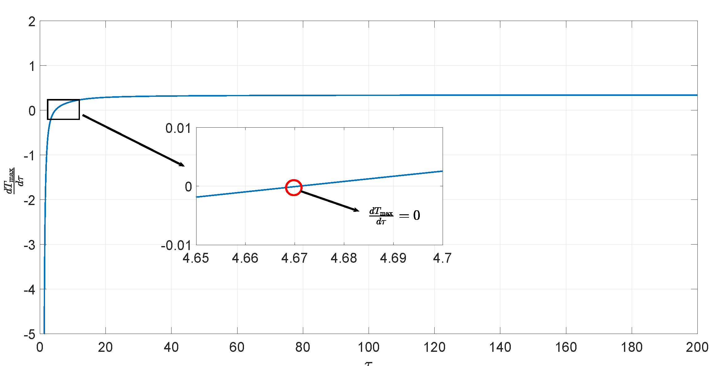
it may be greater than or less than zero. In order to determine the selection strategy of τ, let and draw the image of .
From Figure 2, it notes that for and for . Then, we have the selection strategy of τ: (1)For , the larger τ is, the smaller is. (2)For , the larger τ is, the larger is.
Remark 2.
According to the proof of lemma 1, 2 and 3 in [7,12], it is not difficult to find that, they all ignored a certain term when they estimate the upper bound of convergence time. However, our method takes the form of piecewise function, which makes the upper bound of our estimation closer to the least upper bound.
4. Numerical Simulation and Application
In the part, an application are used to show the validity of fixed-time ZNN model (12).
For (Section 3), chooses , , , , for , and , for , and .
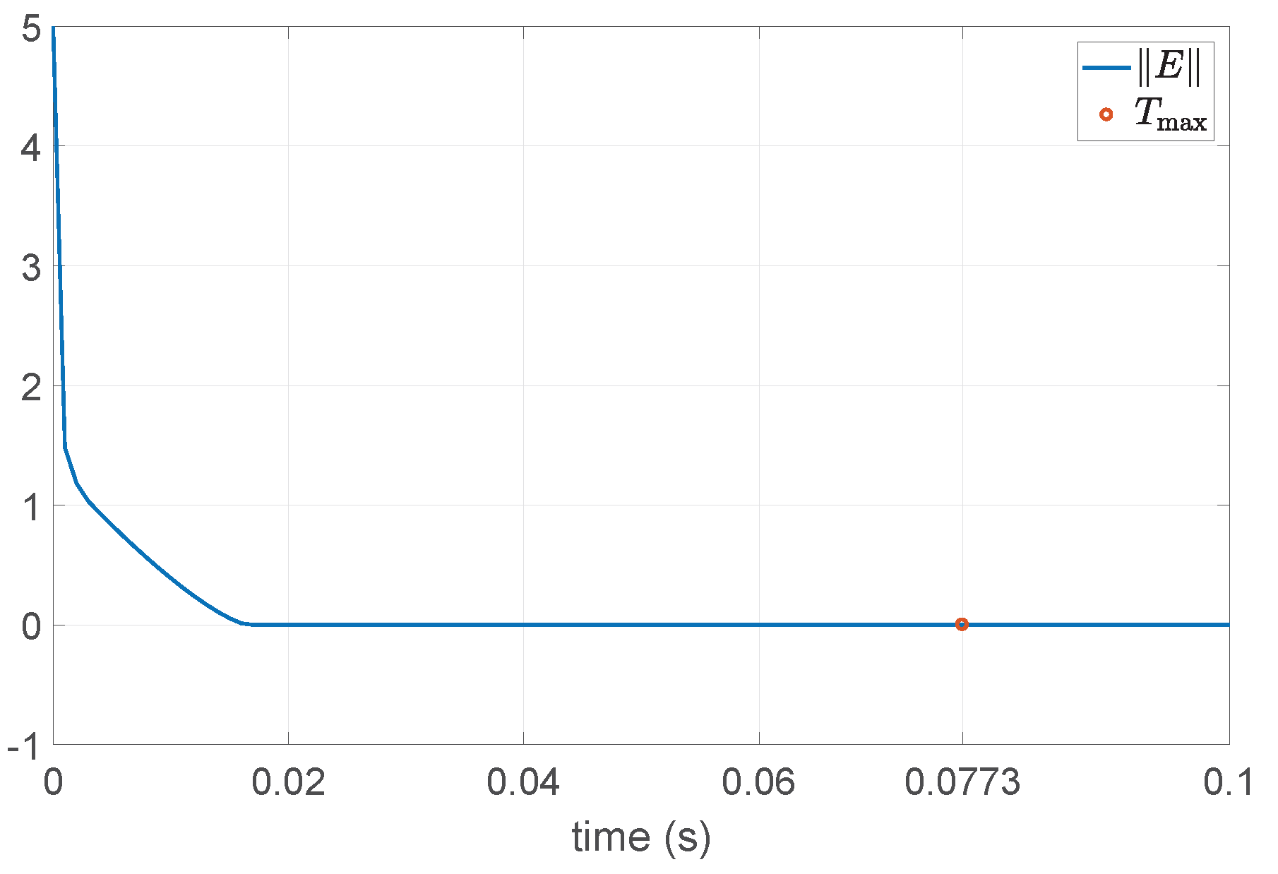
In simulation, we set and . By computing (13), . Figure 3 shows the result. The solution of (Section 3) can be obtained before .
Remark 3.
Compared with traditional LiDAR and visual sensing methods, the proposed fixed-time ZNN model achieves a much shorter response time. Meanwhile, different from conventional finite-time ZNNs whose convergence time is affected by initial states, this model maintains a fixed convergence upper bound regardless of initial error values, which greatly enhances the stability and reliability in dynamic and complex driving scenarios.
Remark 4.
The selected parameters and follow the parameter selection strategies discussed in Remark 1 of Section 3. Under this parameter combination, the model balances convergence speed and numerical stability well. In practical engineering deployment, users can adjust ε and τ according to the real-time requirements of autonomous driving systems: increasing ε can further shorten the convergence time, while a reasonable selection of τ can avoid numerical oscillation in extreme error conditions.
5. Conclusions
This paper proposes a novel fixed-time zeroing neural network and applies it to the real-time inter-vehicle distance estimation task for autonomous driving. A specially designed piecewise activation function is embedded into the ZNN framework, which effectively accelerates the network convergence. Theoretical analysis strictly proves the fixed-time stability of the proposed model, and a tight upper bound of the convergence time is derived analytically. In addition, we systematically analyze the influence of key parameters on the convergence performance and present targeted parameter selection strategies for practical engineering deployment. Numerical simulation results fully validate the superior performance of the proposed method in terms of convergence speed and fixed-time convergence capability. For future research, we will extend the proposed ZNN model to complex traffic scenarios involving multiple vehicles and obstacles. Meanwhile, we will further optimize the activation function to enhance the model’s anti-noise ability and adaptability to extreme driving environments, so as to promote the practical engineering application of ZNN in autonomous driving perception systems.
Author Contributions
D.W. Conceptualization, Methodology, Software, Validation, Investigation, Resources, Data curation, Writing-original draft, Visualization, Project administration, Funding acquisition. P.M. Methodology, Software, Validation,Formal analysis, Investigation, Resources, Data curation, Supervision. All authors have read and agreed to the published version of the manuscript.
Data Availability Statement
All data has been provided in the paper.
Acknowledgments
This work was supported by the Key Scientific Research Foundation of Education Bureau of Henan Province, China (Grant No.25B110021). We would like to express our gratitude to the editor and the anonymous reviewer for their insightful comments.
Conflicts of Interest
The authors have declared no conflict of interest.
References
- Zhang, Y.; Ge, S. S. Design and analysis of a general recurrent neural network model for time-varying matrix inversion[J]. IEEE Trans. Neural Netw. 2005, 16(6), 1477–1490. [Google Scholar] [CrossRef] [PubMed]
- Wang, L.; Miao, P. A novel fixed-time ZNN model and application to robot trajectory tracking[J]. Electron. Lett. 2024, 60(12), e13253. [Google Scholar] [CrossRef]
- Jin, J.; Chen, W.; Chen, C.; et al. A predefined fixed-time convergence ZNN and its applications to time-varying quadratic programming solving and dual-arm manipulator cooperative trajectory tracking[J]. IEEE Trans. Ind. Inform. 2022, 19(8), 8691–8702. [Google Scholar]
- Lu, H.; Jin, L.; Zhang, J.; et al. New joint-drift-free scheme aided with projected ZNN for motion generation of redundant robot manipulators perturbed by disturbances[J]. IEEE Trans. Syst. Man. Cybern. Syst. 2019, 51(9), 5639–5651. [Google Scholar]
- Dai, J.; Chen, Y.; Xiao, L.; et al. Design and analysis of a hybrid GNN-ZNN model with a fuzzy adaptive factor for matrix inversion[J]. IEEE Trans. Ind. Inform. 2021, 18(4), 2434–2442. [Google Scholar]
- Zhang, B.; Zheng, Y.; Li, S.; et al. Fixed-time convergence ZNN model for solving rectangular dynamic full-rank matrices inversion[J]. Expert Syst. With Appl. 2024, 251, 123992. [Google Scholar] [CrossRef]
- Miao, P.; Zheng, Y.; Li, S. A new FXTZNN model for solving TVCS equation and application to pseudo-inverse of a matrix[J]. Appl. Math. Comput. 2024, 465, 128409. [Google Scholar] [CrossRef]
- Li, W.; Wu, H.; Jin, L. A Lower Dimension Zeroing Neural Network for Time-Variant Quadratic Programming Applied to Robot Pose Control[J]. IEEE Transactions on Industrial Informatics, 2024. [Google Scholar]
- Jin, L.; Zhang, Y.; Li, S.; et al. Modified ZNN for time-varying quadratic programming with inherent tolerance to noises and its application to kinematic redundancy resolution of robot manipulators[J]. IEEE Trans. Ind. Electron. 2016, 63(11), 6978–6988. [Google Scholar] [CrossRef]
- Wen, H.; Qu, Y.; He, X.; et al. First/second-order predefined-time convergent ZNN models for time-varying quadratic programming and robotic manipulator application[J]. ISA Trans. 2024, 146, 42–49. [Google Scholar] [CrossRef] [PubMed]
- Polyakov, A. Nonlinear feedback design for fixed-time stabilization of linear control systems[J]. IEEE Trans. Autom. Control 2011, 57(8), 2106–2110. [Google Scholar]
- Hu, C.; Yu, J.; Chen, Z.; et al. Fixed-time stability of dynamical systems and fixed-time synchronization of coupled discontinuous neural networks[J]. Neural Netw. 2017, 89, 74–83. [Google Scholar] [CrossRef] [PubMed]
- Chen, C.; Li, L.; Peng, H.; et al. A new fixed-time stability theorem and its application to the fixed-time synchronization of neural networks[J]. Neural Netw. 2020, 123, 412–419. [Google Scholar] [CrossRef] [PubMed]
- Miao, P.; Li, S.; Li, C. Tracking problem of non-particle morphology based on fixed-time ZNN model[J]. Math. Comput. Simul. 2025, 238, 189–200. [Google Scholar] [CrossRef]
- Zhang, Y.; Ma, W.; Cai, B. From Zhang neural network to Newton iteration for matrix inversion[J]. IEEE Trans. Circuits Syst. I Regul. Pap. 2008, 56(7), 1405–1415. [Google Scholar]
- Xiao, L.; Zhang, Y. Zhang neural network versus gradient neural network for solving time-varying linear inequalities[J]. IEEE Trans. Neural Netw. 2011, 22(10), 1676–1684. [Google Scholar] [CrossRef] [PubMed]
- Li, S.; Chen, S.; Liu, B. Accelerating a recurrent neural network to finite-time convergence for solving time-varying Sylvester equation by using a sign-bi-power activation function[J]. Neural Process. Lett. 2013, 37, 189–205. [Google Scholar]
- Shen, Y.; Miao, P.; Huang, Y.; et al. Finite-time stability and its application for solving time-varying Sylvester equation by recurrent neural network[J]. Neural Process. Lett. 2015, 42, 763–784. [Google Scholar]
- Miao, P.; Shen, Y.; Xia, X. Finite time dual neural networks with a tunable activation function for solving quadratic programming problems and its application[J]. Neurocomputing 2014, 143, 80–89. [Google Scholar] [CrossRef]
Figure 1.
Autonomous driving schematic diagram and mathematical model diagram.
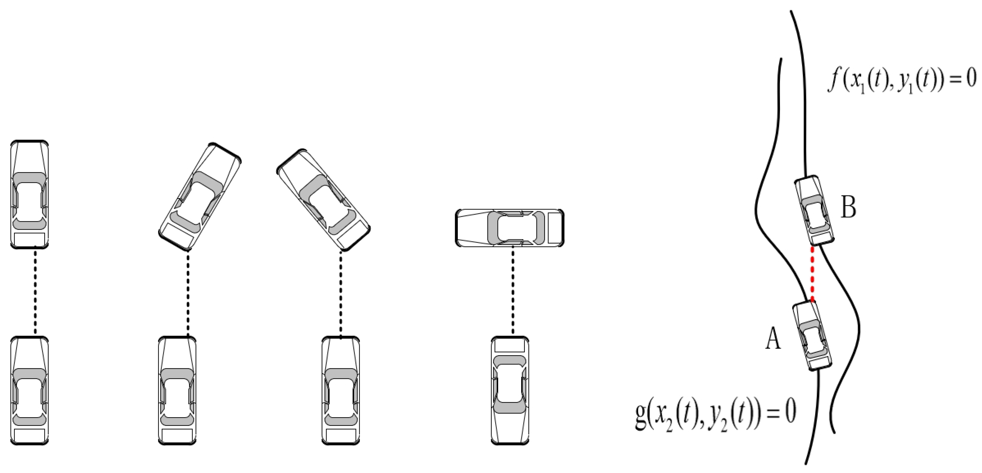
Figure 2.
The value of for .
Disclaimer/Publisher’s Note: The statements, opinions and data contained in all publications are solely those of the individual author(s) and contributor(s) and not of MDPI and/or the editor(s). MDPI and/or the editor(s) disclaim responsibility for any injury to people or property resulting from any ideas, methods, instructions or products referred to in the content. |
© 2026 by the authors. Licensee MDPI, Basel, Switzerland. This article is an open access article distributed under the terms and conditions of the Creative Commons Attribution (CC BY) license (http://creativecommons.org/licenses/by/4.0/).
Copyright: This open access article is published under a Creative Commons CC BY 4.0 license, which permit the free download, distribution, and reuse, provided that the author and preprint are cited in any reuse.


