

Submitted:
08 August 2026
Posted:
10 August 2026
You are already at the latest version
Abstract
Cold-pool structure controls the confinement and transport environment relevant to surface wintertime ozone in the mountainous Uinta Basin, Utah, USA, but point surface values alone do not establish that structure. We evaluated deterministic responses in Weather Research and Forecasting (WRF) simulations of the 2 February 2013 high-ozone episode to the supplied Global Forecast System (GFS) or North American Model (NAM) driving analyses, nest feedback, boundary-layer and surface-layer treatment, slope-aware radiation, and terrain source/resolution. Across a common five-hour sample, GFS-driven members were warmer at the evaluated surface sites, less stable in the lowest 500 m, and marginally stronger fixed-layer advection than matched NAM members. All GFS-driven runs retained a weaker cold pool, defined as a smaller vertically integrated heat deficit; every simulation gained heat deficit (strengthened the cold pool) over the retained window. Results suggest the driving product (GFS, NAM) in this case study made more difference to cold-pool generation than other changes in WRF by an order of magnitude. Responses to feedback, parameterisation variation were negligible, while the fineness of terrain modulated the speed of cold-pool formation likely due to a lower roughness in coarse orography. The meteorological results, a longtime impediment to local air-chemistry forecasts, advise subsequent air-chemistry modelling on ingesting the necessary cold pool, trapping precursors and pollutants.
Keywords:
ozone
; WRF
; meteorology
; modelling
; cold-air pool
; complex terrain
; model resolution
1. Introduction
Surface wintertime ozone in the Uinta Basin develops within a snow-covered, persistently stable boundary layer in which weak mixing and transport can confine precursors near the surface [1,2,3]. The Basin hosts an active oil and gas industry, while its altitude encourages stratospheric (ozone-rich) intrusions to lower levels, creating a unique problem not always implicit in national regulation. For a coupled weather–chemistry calculation, the relevant meteorological information extends beyond 2 m temperature to the simulated depth, stability, and transport of the lower atmosphere. For the Basin, a persistent cold pool and high surface albedo promotes substantial photolysis in adequate insolation; the temperature inversion trapping this mixture is essential at time zero for a chemical model to possibly reproduce surface-measured ozone levels. Indeed, while point observations remain indispensable, a horizontally separated surface network does not by itself validate inversion depth or the three-dimensional mixing volume supplied to chemistry.
Meteorological, emission inventory, photolysis, deposition, and chemical-mechanism errors can cancel or amplify in coupled simulations. For example, holding meteorology fixed while changing emissions can alter ozone agreement without identifying a unique inventory error [1]. Cumulative changes in emissions, leaf area, deposition, and meteorology likewise complicate attribution, and improved modelled temperature profiles need not translate directly into improved ozone profiles [4]. Credible meteorology is thus a prerequisite for chemical attribution rather than proof that meteorology is the dominant or only uncertainty; unpublished work within the laboratory has show this is a long-standing impediment to accurate simulations of this particular case chosen due to its place in an intense observation period (IOP) [2].
Previous unpublished preliminary WRF experiments suggest en masse snow, microphysics, and grid choices can produce large case-specific responses, while evaluation and chemistry grids need not sample the same structure [2]. Four-dimensional data-assimilation responses can depend on the nudged variables, input data, and PBL-scheme-dependent boundary-layer diagnosis [5].
Following preliminary experiments and review of the simulations, we ask:
- 1.
- Does the lower-layer response to the supplied GFS or NAM driving analysis recur under both one-way and two-way nest feedback?
- 2.
- How large are the nest-feedback, parameterisation-variation, and slope-radiation responses relative to the driving NWP product’s response on common diagnostics?
- 3.
- What effect may terrain fineness in the NWP model have on cold-pool formation?
- 4.
- What do surface, common-height, and footprint heat-deficit diagnostics reveal together that any single station metric can miss, and how does this impact downstream numerical chemical forecasts?
The simulations use X0–X10 identifiers, which link configurations in the text and tables to the run inventory (Table XX). Note the present paper evaluates the meteorological state that a later chemistry calculation would receive; it contains no chemistry calculation and makes no ozone prediction.
2. Materials and Methods
2.1. Case, Observations, and Evaluation Domains
The case is 2 February 2013 within a broader January–February period of snow cover, cold-pool conditions, and elevated ozone in the Uinta Basin [1,2,5]. The WRF integrations cover 1200–1800 Coordinated Universal Time (UTC), corresponding to 0500–1100 Mountain Standard Time (MST; UTC). The retained analysis window covers 1400–1800 UTC, or 0700–1100 MST, and excludes both the 1200 UTC initialised output and the 1300 UTC first-hour forecast, leaveing five hourly samples for the common window. Surface observations were obtained via Synoptic Data (https://docs.synopticdata.com/services/, accessed 1 June 2026) via python package SynopticPy (https://github.com/blaylockbk/SynopticPy, accessed 1 June 2026) for 2 m temperature at 11 sites, 10 m wind speed at 10 sites, and surface pressure at 9 sites. Subhourly reports were mean-averaged within each UTC clock hour. The stations span basin-floor, sidewall, and bench locations but are neither spatially uniform nor area weighted; as the focus herein is not verification against observations, we leave further evaluation to future studies. The 1 km (middle) domain was selected for the common observation comparisons because seven stations fall outside the innermost domain, leaving four intersecting station datasets in the finest-resolution region. Figure 1 combines the reporting-station geometry with the full nested-domain layout. Observed and modelled surface potential temperature for a two-site structural index was calculated as , with T in kelvin and p in hPa. The index is Mountain Home on the north-west bench minus Pariette Draw on the basin floor, with both locations labelled in Figure 1. Their horizontal separation requires treating the index as a surface contrast rather than free-air inversion strength or cold-pool depth. Further work on pseudo-lapse-rates (i.e., temperature profiles in the absence of radiosonde launches) is discussed in [6] and [7].
Episode-scale ozone context came from the US Environmental Protection Agency (EPA) Air Quality System (AQS) AirData daily archive for 1 January–28 February 2013. We retained the 8-hour-mean daily-summary row at Ouray, Redwash, Roosevelt, Vernal, and Little Mountain (Figure 1). The satellite panel in Figure 2 uses the National Aeronautics and Space Administration (NASA) Global Imagery Browse Services (GIBS) Terra Moderate Resolution Imaging Spectroradiometer (MODIS) corrected-reflectance 7-2-1 layer for 2 February 2013, acquired from https://worldview.earthdata.nasa.gov/ (accessed 1 June 2026).
2.2. WRF Configuration and Archived Simulation Family
The six-hour simulations used WRF version 4.8.0 [8], initialised at 1200 UTC with either Global Forecast System (GFS) or North American Model (NAM) analyses and supplied with analysis-derived lateral boundary conditions through to 1800 UTC on 2 February 2013. These are retrospective simulations driven by analyses rather than six-hour operational forecasts, and the design does not separate the initialised state from the subsequent lateral-boundary contribution. We used three nested computational domains, named d01–d03, with horizontal grid spacings of 3 km, 1 km, and 333.333 m, respectively. All runs prescribe 75 eta model levels concentrated near the surface, with approximately 20 m separation among the lowest mass levels, and a 50 hPa model top. The reference physics suite used Thompson microphysics, Rapid Radiative Transfer Model for General Circulation Models (RRTMG) longwave and shortwave radiation, the revised fifth-generation Pennsylvania State University–National Center for Atmospheric Research Mesoscale Model (MM5) similarity surface layer, the Noah land-surface model, and the Yonsei University (YSU) planetary boundary layer (PBL) scheme [9,10,11,12,13]. Grid and observation four-dimensional data assimilation (e.g., nudging deployed in [5] were disabled. Departures from the reference configuration are listed by simulation in Table 1.
Terrain fineness entered through the WRF Preprocessing System (WPS); the fine source used 3-arc-second terrain, the WRF-default (medium) source was 30-arc-second class, and the coarse source used the 5-arc-minute GMTED2010 product. At approximately N nominal north–south spacing in the terrain grid are about 90 m, 900 m, and 9 km, respectively; these static-source spacings are distinct from WRF horizontal grid spacing. Land-surface initial fields, including snow, entered through the source-specific meteorological preprocessing, so the GFS–NAM treatment does not isolate a snow-field contribution.
2.3. Controlled Contrasts
We contrast simulations, identifying the dominant dial on the simulation’s sensitivity, and its magnitude (Table 2). The four default-terrain simulations X3, X5, X6, and X10 form a basic two-by-two comparison that buttresses our analyses. For all experiments, native GFS and NAM data provides 27 and 40 metgrid levels, respectively.
2.4. Surface and Common-AGL Diagnostics
Modelled 2 m dry-bulb temperature, 10 m wind, and surface pressure were sampled at the nearest d02 cell to each station. None of the selected cells lay on steep terrain or an obviously unrepresentative model location. Across the eleven fixed columns, model terrain offset from reported station elevation spanned -32 m to 14 m. While this justifies the nearest-neighbour approach, the pairing of WRF output to observation value does not remove (wind, solar) exposure, slope angle, land-cover use, or network-coverage deficiency. Mass-level height above ground level (AGL) was calculated from perturbation plus base geopotential relative to local WRF terrain height. Grid-relative winds were destaggered and rotated to earth-relative components. Model-level potential temperature and horizontal wind components were interpolated linearly at 25 m increments from 50 to 500 m AGL at each station column; fixed-layer stability was then defined as
The transport-wind proxy was defined as
where the bars denote height means from 50 to 500 m AGL. This wind-derived quantity is a fixed-layer transport proxy and does not sample flow through a basin boundary, pollutant residence time, cold-pool volume, or a chemistry-model ventilation coefficient. Native WRF PBL height was retained only as a scheme-dependent companion diagnostic, consistent with the diagnostic cautions discussed by Tran et al. [5].
2.5. Pairing, Aggregation, and Short-Sample Sensitivity
Run differences were paired by station and valid hour before spatial aggregation. Each fixed station field was reduced to a single unweighted spatial median per hour; the five-hour value is thus a mean of those five medians. Because this is one deterministic case, interpretation emphasises practical significance and surprises, rather than broader, statistical significance.
2.6. Integrated Heat Deficit as Measure of Cold Pool Strength
We calculated a crest-referenced atmospheric heat-deficit proxy following the basin-volume formulation of [14] and closest column method in [15]. Let and denote the pressures at the surface and fixed crest reference, respectively, with . For there, area-normalised atmospheric heat-deficit was defined as , where is the potential temperature interpolated to the crest height in each modelled column. H is reported as the cell-area-weighted and vertically integrated heat deficit in MJ m−2. The footprint of cells is the convex hull of eleven evaluation stations intersected with model terrain below the 2200 m crest reference (4,965 d02 cells and 5,277 km2). We tested sensitivity of interpretation of results to crest definition by varying "crest height" between 2100, 2200, and 2300 m in preliminary work. This confirmed robustness of the nominal height. Finally, note the integrated footprint area is an evaluation region rather than a hydrologic basin boundary.
3. Results
3.1. Observed Episode Context
The MODIS browse image shows extensive snow and/or ice across the Uinta Basin and surrounding terrain on 2 February (Figure 2a). The air-quality time series places the simulation date within a broader period of elevated daily ozone maxima (Figure 2b). On 2 February, the reported daily maximum eight-hour values were 56 ppb at Little Mountain, 65–70 ppb at Vernal and Roosevelt, 81 ppb at Redwash, and 95 ppb at Ouray.
3.2. Observed Surface-Temperature Context
The basin-floor station disconnected overnight from the higher sites between 31 January and 3 February; accordingly, the magnitude and ordering of station temperatures evolved through the diurnal cycle (Figure 3). The recurring floor-to-bench separation is consistent with a cold-pool surface pattern. Because the stations are horizontally separated, however, the time series do not determine the cold-pool top, depth, volume, or vertical temperature structure. This motivates three-dimensional simulations that reveal such structures to a sufficient level of fidelity to reproduce high-ozone cases in the Basin.
3.3. Common-Pipeline Contrasts at a Glance
Figure 4 compares all sensitivity tests; evidently, the two driving-product contrasts are the shot-callers in temperature, fixed-layer stability, and transport wind. The PBL/surface-layer treatment is smaller, while slope radiation and nest feedback impacts are near zero. Pressure and wind-error metrics follow different orderings, and do not offer a consistent narrative to add to the previous inferences with confidence.
3.4. Driving-Product Response in the Lower Layer
The two-by-two matrix in Figure 5 separates the GFS-versus-NAM driving-product response under one-way and two-way feedback. Evidence includes:
- Relative to GFS, NAM was 3.63 K more stable with two-way feedback and 3.65 K more stable with one-way feedback through the 50–500 m layer (Table A1).
- The five-hour means of hourly spatial-median stability were 7.50 and 7.38 K for the two GFS runs, compared with 10.82 K for both NAM members.
- The hourly GFS-minus-NAM differences ranged from to K with two-way feedback and from to K with one-way feedback.
All ten product-by-hour stability contrasts therefore retained the same sign and provide some confidence of a genuine signal. Further,
- GFS also increased fixed-layer transport wind by 0.79 m s−1 with two-way feedback and 0.99 m s−1 with one-way feedback.
- The corresponding five-hour means of hourly spatial-median transport wind were approximately 2.0 m s−1 for both GFS members and approximately 1.1 m s−1 for both NAM members.
- The hourly differences ranged from 0.37 to 1.18 m s−1 with two-way feedback and from 0.61 to 1.50 m s−1 with one-way feedback, with the same sign in every hour.
Native PBL-height differences changed sign within both feedback modes and did not reproduce the stability and wind separation, hence lower confidence in initial interpretation. This divergence is also consistent with the scheme dependence of native PBL-height diagnosis discussed by Tran et al. [5].
3.5. Surface and Spatial Corroboration
In temperature — perhaps the key sensible meteorological variables for the case — GFS-minus-NAM 2 m temperature-bias contrasts were +1.79 °C with two-way feedback and +1.76 °C with one-way feedback (Table A2). Surface-pressure absolute-error contrasts changed in the opposite direction, at and Pa, while hourly wind absolute-error differences changed sign. No single surface score therefore provides a general product ranking. Figure 6 gives a separate two-site surface-structure comparison for the observations and two-way-feedback simulations.
The five-hour mean surface potential-temperature contrast between Mountain Home and Pariette Draw was 16.94 K in the observations, 17.03 K in NAM two-way, and 9.95 K in GFS two-way. The close NAM value somewhat corroborates this (albeit surface-based) index. Across the registered footprint, the mean GFS-minus-NAM near-surface response was positive and the vertical response remained concentrated below 500 m AGL under both feedback modes (Table A2). In terms of robustness, only 64–67% of footprint cells had the same sign at 1400–1500 UTC, lowering weight of confidence in these values. The result is therefore shallow and mean-coherent, but not spatially uniform throughout the retained window; later hours were more coherent, however.
3.6. Heat Deficit: A Weaker State without Faster Loss
The GFS runs retained less area-mean, vertically integrated heat deficit at every retained hour under all seven definitions (Section 2.6; Table A3): a weaker cold pool. Mean GFS-minus-NAM differences were MJ m−2, while every run gained heat deficit from 1400 to 1800 UTC (strengthened the cold pool). We conclude therefore that the weaker GFS cold pool did not result from faster heat-deficit loss during the window. Figure 7 shows the four increasing trajectories and the persistent separation between the two GFS and two NAM members.
3.7. Process Treatments on the Fine-Terrain Branch
The MYJ/Eta versus YSU/revised-MM5 scheme pair changes only the PBL and surface-layer schemes while holding the fine terrain and slope-aware-radiation configuration fixed. MYJ/Eta increased 2 m-temperature bias by 0.37 °C, reduced 10 m-wind absolute error by 0.145 m s−1, and increased fixed-layer transport wind by 0.098 m s−1, with the same sign in all five hours increasing the authors’ confidence in fidelity. These changes are noticably smaller than the driving-product response on these lower-layer metrics; a lack of pattern in temperature- and wind-error changes do not support an overall scheme-skill ranking, which must be saved for future work and statistical testing.
The slope-radiation addition produced negligible response at the basin-floor station columns. A spatially organised skin-temperature response appeared on the sidewalls, but the archived flat-plane shortwave field and missing surface heat fluxes could not test the mechanism directly (not shown).
3.8. Nest-Feedback Robustness across Two Terrain Regimes
Feedback effects were small for both GFS and NAM: WRF driving from coarsest to finest grid top-down is therefore least noisy, more stable, and computationally more efficient (drawing from the rationale of WRF software operation). The fine-terrain NAM pair reproduced that character: two-way minus one-way feedback increased stability by 0.04 K and reduced transport wind by 0.01 m s−1. The 10 m-wind and surface-pressure changes were small and do not support confident conclusions beyond this five-hour case.
3.9. Terrain Fineness
The terrain-resolution tests Figure 8 hold NAM forcing, one-way feedback, WRF grid spacing, and the YSU/MM5 physics configuration fixed while changing only the terrain fineness. Analysing difference plots revealed default-minus-fine response was small on d02, where the Basin can be seen in full (not shown). The coarsest terrain produced larger spatial responses, albeit unrealistically coarse compared with operational models, but accentuate the impacts.
4. Discussion
4.1. Main Driver of Variance in Low-Level State is Choice of NWP Input
The present study suggests repeated difference in the lower-layer state seen in simulations, supplied by the two driving products of GFS and NAM, dictate an order of magnitude more variance than other factors studied herein. Moreover,
- The GFS-driven runs supplied a warmer, less stable, and faster-moving 50–500 m layer than feedback-matched NAM members.
- The heat-deficit calculation reproduced the same ordering after varying footprint area of the integration (not shown).
- Surface pressure and wind error followed different orderings, precluding an inferred skill ranking.
The GFS state is more consistent with weaker confinement of notional pollutant precursors than the analogous NAM state; however, the transport-wind proxy and heat-deficit values are not substitutes for measured mixing volume or basin export. This distinction matters because errors in confinement, emissions, snow and cloud processes, photolysis, deposition, and chemical mechanism can compensate for one another in coupled simulations [1,2,4]. A practical future ensemble should therefore vary the treatments that show the largest phenomenon-relevant response, but the present single case cannot advise or prescribe a universal design: this is planned subsequent work.
The model-only d03 Horsepool profiles at 1200 and 1300 UTC (Figure 9) expose the source-specific supplied states and their first-hour evolution. (Note they do not separate early model adjustment from lateral-boundary evolution.)
4.2. Initial State Offset, not Cold-Pool Loss, Dictates Variation
The heat-deficit result narrows the interpretation: GFS had less deficit than NAM, but deficit increased in every simulation during the retained window (Figure 7). This undermines the idea of theoretical erosion of the cold pool ("heat-deficit loss") would yield a weaker cold pool after spin-up. Indeed, a longer integration through at least one complete diurnal cycle is required to test whether the products differ in cold-pool erosion or persistence. The spatial analysis gives a similarly bounded result: responses were strongest below 500 m AGL and had consistent bias (over/under) every hour, increasing confidence.
4.3. Secondary Experiments Narrow Rather than Expand the Claim
The secondary comparisons delimit the driving-product result rather than expanding it into a configuration ranking:
- Figure 4 shows that the driving-product contrasts are strongestin2-m temperature, low-level stability, and transport-wind metrics.
- The boundary-layer/surface-layer treatment produced a coherent but smaller response: temperature bias increased while wind absolute error decreased.
- Nest-feedback effects remained small on both default- and fine-terrain branches, providing a five-hour robustness check rather than evidence that feedback is generally unimportant.
- The slope-radiation response was negligible at the station columns, while the supplementary sidewall diagnostic shows a spatially organised response that the station metric missed.
- Reducing terrain resolution suggests a faster cold-air drainage due to a smoother surface, but lower volume of cold air.
4.4. Observation and Design Limits Set the Next Experiment
These outcomes motivate better measurements and future experiment design, but they do not support rigorous claims of an optimal namelist: rather, starting points. Two limitations are especially important for the next experiment:
- Native PBL height is scheme dependent. MYJ and YSU need not diagnose the layer top in the same way, so common-height stability and transport remain the more comparable quantities.
- The floor-to-bench temperature contrast is not vertical validation. Independent profiles are required to evaluate inversion depth, layer stability, and modelled heat deficit.
A future intense observation period may remove the obstacle of fine-scale verification, including the pseudo-lapse-rate calculations important for measuring and predicting inversion strength/breakup and pollutant dispersion.
5. Conclusions
The largest response is the GFS-versus-NAM driving-product contrast: relative to NAM, GFS is warmer at the evaluated surface sites, about 3.6 K less stable at low levels, about 1.0 m s−1 strong wind in fixed-layer transport, and a weaker cold pool as measured by vertically integrated heat deficit. The heat-deficit separation is therefore likely a state offset, not demonstrated faster loss via entrainment, transport, etc; and the surface metrics do not support a universal product ranking. Nest-feedback effects are much smaller, the PBL/surface-layer response is smaller and metric dependent, and the slope-radiation and fine-terrain responses do not support configuration-superiority claims. However, the dependence of cold-pool formation speed and strength indicate a fruitful and informative line of new research for numerical modelling of air quality in complex terrain.
In future work, experiment design may separatesinitial from lateral-boundary forcing. Further, the results herein do not identify the responsible product component, validate inversion depth, establish event-scale persistence, calculate basin export, or predict ozone. Within those bounds, nonetheless, the driving-product variation in NWP source produced the largest consistent differences in the lower-basin meteorological state supplied to downstream chemistry during the five-hour window.
The numerical summaries supporting the concise Results narrative are retained in Appendix A.
Author Contributions
John R. Lawson: Conceptualization, Methodology, Software, Validation, Formal analysis, Investigation, Data curation, Writing—original draft, Writing—review and editing, Visualisation, and Project administration; Michael J. Davies: Methodology, Software, Validation, Formal analysis, Investigation, Data curation, Visualisation, and Writing—review and editing; Loknath Dhar: Conceptualization, Resources, and Writing—review and editing; Seth N. Lyman: Conceptualization, Writing—review and editing, Supervision, Project administration, and Funding acquisition.
Funding
Funding was provided by the Utah Legislature and Uintah County Special Service District 1. The article processing charge was waived. The funders had no role in the design of the study; in the collection, analyses, or interpretation of data; in the writing of the manuscript; or in the decision to publish the results.
Institutional Review Board Statement
Not applicable.
Informed Consent Statement
Not applicable.
Data Availability Statement
The analysis scripts, derived hourly and paired summaries, heat-deficit tables, selected EPA AQS daily records, run and comparison inventories, provenance records, and promoted figures used for this draft are retained in the private working repository at www.github.com/bingham-research-center. Raw WRF inputs and Synoptic observations remain subject to the respective providers’ access and reuse terms.
Acknowledgments
We acknowledge the University of Utah Center for High Performance Computing for computational resources. We acknowledge Synoptic Data PBC for access to Mesonet API observations. We thank Brian K. Blaylock for the Herbie and SynopticPy packages, which supported source-data retrieval and Synoptic API access, respectively (Herbie: https://doi.org/10.5281/zenodo.4567540; SynopticPy: https://doi.org/10.5281/zenodo.4567546). We thank Pamela Gardner for editorial and funding advice and KarLee Zager for continued contributions to collecting data relevant to this project.
Conflicts of Interest
The authors declare no conflict of interest.
Use of Artificial Intelligence
Generative artificial intelligence tools, including Anthropic Claude and OpenAI Codex, were used during manuscript preparation to assist with literature synthesis, provenance and analysis-code review, and drafting and editing. The authors reviewed and edited the resulting material and take responsibility for the content.
Appendix A. Data Tables and Secondary Diagnostics
This appendix retains the core numerical detail supporting the concise Results narrative.

Table A1.
Paired effects for the default-terrain driving-product/feedback matrix, averaged over the five hourly spatial medians. Positive temperature values indicate a warmer model-minus-observation bias, positive stability values indicate a more stable fixed layer, and positive transport-wind values indicate a larger layer-mean wind. The effects are deterministic descriptive contrasts rather than inferential estimates.
Table A1.
Paired effects for the default-terrain driving-product/feedback matrix, averaged over the five hourly spatial medians. Positive temperature values indicate a warmer model-minus-observation bias, positive stability values indicate a more stable fixed layer, and positive transport-wind values indicate a larger layer-mean wind. The effects are deterministic descriptive contrasts rather than inferential estimates.
| Effect | T2 bias (°C) | (K) | (m s−1) |
|---|---|---|---|
| GFS − NAM, two-way | +1.79 | -3.63 | +0.79 |
| GFS − NAM, one-way | +1.76 | -3.65 | +0.99 |
| GFS one-way − two-way | +0.07 | -0.07 | +0.10 |
| NAM one-way − two-way | -0.01 | +0.00 | +0.01 |
| Feedback interaction | +0.04 | -0.10 | +0.10 |
Table A2.
Surface, spatial, and vertical corroboration for the two GFS-minus-NAM driving-product contrasts. Every value uses the matched station and hour samples described in Section 3.5.
Table A2.
Surface, spatial, and vertical corroboration for the two GFS-minus-NAM driving-product contrasts. Every value uses the matched station and hour samples described in Section 3.5.
| Diagnostic | Result | Scope |
|---|---|---|
| 2 m temperature | GFS-minus-NAM bias contrast +1.79 °C two-way and +1.76 °C one-way; absolute-error differences +1.41 and +1.50 °C | Same ordering as common-AGL stability |
| 10 m wind | Bias contrast +0.91 and +0.96 m s−1; hourly absolute-error differences change sign | No stable wind-skill ordering |
| Surface pressure | Absolute-error contrast -13.6 Pa two-way and -10.9 Pa one-way; negative in every hour | Opposite ordering from temperature, with small absolute differences |
| Two-site surface index | Observed 12.63–20.21 K; NAM 16.44–18.07 K; GFS 7.35–11.74 K under two-way feedback | Horizontally separated surface contrast, not inversion strength or depth |
| Mean 2 m potential-temperature difference | +0.89 to +1.16 K at 1400–1500 UTC; +2.00 to +2.74 K at 1600–1800 UTC | Positive at all ten pair-hours |
| Footprint sign share | 0.64–0.67 at 1400–1500 UTC; 0.84–0.93 later | Early response is not spatially uniform |
| Low-to-aloft absolute-response ratio | 1.45–3.12 | Response concentrated in the lower atmosphere |
| 50–500 m stability difference | -4.33 to -3.04 K | Negative at all ten pair-hours |
Table A3.
Footprint-mean, vertically integrated heat-deficit contrasts over the 1400–1800 UTC decision window. The primary definition uses the combined station-and-waypoint hull with a 2200 m crest (4965 cells, 5277 km2); envelopes span all seven footprint definitions. The values are deterministic descriptive contrasts in MJ m−2.
Table A3.
Footprint-mean, vertically integrated heat-deficit contrasts over the 1400–1800 UTC decision window. The primary definition uses the combined station-and-waypoint hull with a 2200 m crest (4965 cells, 5277 km2); envelopes span all seven footprint definitions. The values are deterministic descriptive contrasts in MJ m−2.
| GFS − NAM quantity | Two-way pair | One-way pair |
|---|---|---|
| Mean difference (primary) | -1.23 | -1.25 |
| Hourly range (primary) | -1.50 to -0.97 | -1.53 to -0.99 |
| Hourly envelope (seven definitions) | -1.77 to -0.70 | -1.80 to -0.71 |
| GFS change, 1400–1800 UTC | +0.32 | +0.30 |
| NAM change, 1400–1800 UTC | +0.15 | +0.13 |
| Difference in change (primary) | +0.17 | +0.17 |
References
- Ahmadov, R.; McKeen, S.; Trainer, M.; Banta, R.; Brewer, A.; Brown, S.; Edwards, P.M.; De Gouw, J.A.; Frost, G.J.; Gilman, J.; et al. Understanding high wintertime ozone pollution events in an oil-and natural gas-producing region of the western US. Atmos. Chem. Phys. 2015, 15, 411–429. [Google Scholar] [CrossRef]
- Neemann, E.M.; Crosman, E.T.; Horel, J.D.; Avey, L. Simulations of a cold-air pool associated with elevated wintertime ozone in the Uintah Basin, Utah. Atmos. Chem. Phys. 2015, 15, 135–151. [Google Scholar] [CrossRef]
- Davies, M.J.; Lawson, J.R.; O’Neil, T.; Lyman, S.N.; Zager, K.; Coxson, T.D. Uinta Basin snow shadow: Impact of snow-depth variation on winter ozone formation. Air 2025, 3, 22. [Google Scholar] [CrossRef]
- Matichuk, R.; Tonnesen, G.; Luecken, D.; Gilliam, R.; Napelenok, S.L.; Baker, K.R.; Schwede, D.; Murphy, B.; Helmig, D.; Lyman, S.N.; et al. Evaluation of the Community Multiscale Air Quality Model for Simulating Winter Ozone Formation in the Uinta Basin. J. Geophys. Res. D. Atmos. 2017, 122, 13545–13572. [Google Scholar] [CrossRef] [PubMed]
- Tran, T.; Tran, H.; Mansfield, M.; Lyman, S.; others. Four dimensional data assimilation (FDDA) impacts on WRF performance in simulating inversion layer structure and distributions of CMAQ-simulated winter ozone …. Atmos. Environ. 2018. [Google Scholar] [CrossRef]
- Whiteman, C.D.; Hoch, S.W. Pseudovertical temperature profiles in a broad valley from lines of temperature sensors on sidewalls. J. Appl. Meteorol. Climatol. 2014, 53, 2430–2437. [Google Scholar] [CrossRef]
- Mansfield, M.L. Statistical analysis of winter ozone exceedances in the Uintah Basin, Utah, USA. J. Air Waste Manag. Assoc. 2018, 68, 403–414. [Google Scholar] [CrossRef] [PubMed]
- Skamarock, W.C.; Klemp, J.B.; Dudhia, J.; Gill, D.O.; others. A Description of the Advanced Research WRF Version 3, 2008. NCAR Tech. Note NCAR/TN- 2008 113.
- Thompson, G.; Field, P.R.; Rasmussen, R.M.; Hall, W.D. Explicit forecasts of winter precipitation using an improved bulk microphysics scheme. Part II: Implementation of a new snow parameterization. Mon. Weather Rev. 2008, 136, 5095–5115. [Google Scholar] [CrossRef]
- Iacono, M.J.; Mlawer, E.J.; Clough, S.A.; Morcrette, J.J. Impact of an improved longwave radiation model, RRTM, on the energy budget and thermodynamic properties of the NCAR community climate model, CCM3. J. Geophys. Res. 2000, 105, 14873–14890. [Google Scholar] [CrossRef]
- Jiménez, P.A.; Yang, J.; Kim, J.H.; Sengupta, M.; Dudhia, J. Assessing the WRF-solar model performance using satellite-derived irradiance from the National Solar Radiation Database. J. Appl. Meteorol. Climatol. 2022, 61, 129–142. [Google Scholar] [CrossRef]
- Niu, G.Y.; Yang, Z.L.; Mitchell, K.E.; Chen, F.; Ek, M.B.; Barlage, M.; Kumar, A.; Manning, K.; Niyogi, D.; Rosero, E.; et al. The community Noah land surface model with multiparameterization options (Noah-MP): 1. Model description and evaluation with local-scale measurements. J. Geophys. Res. 2011, 116. [Google Scholar] [CrossRef]
- Hong, S.Y.; Noh, Y.; Dudhia, J. A New Vertical Diffusion Package with an Explicit Treatment of Entrainment Processes. Mon. Weather Rev. 2006, 134, 2318–2341. [Google Scholar] [CrossRef]
- Whiteman, C.D.; Lehner, M.; Hoch, S.W.; others. The nocturnal evolution of atmospheric structure in a basin as a larger-scale katabatic flow is lifted over its rim. [CrossRef]
- Adler, B.; Wilczak, J.M.; Kenyon, J.; Bianco, L.; Djalalova, I.V.; Olson, J.B.; Turner, D.D. Evaluation of a cloudy cold-air pool in the Columbia River basin in different versions of the High-Resolution Rapid Refresh (HRRR) model. Geosci. Model Dev. 2023, 16, 597–619. [Google Scholar] [CrossRef]
Figure 1.
Geographic and sampling orientation for the evaluation. (a) The d02 terrain, reporting stations, and d03 interior define the common evaluation setting. (b) The d01–d02–d03 WRF grid layout places that setting within the full three-domain configuration. Seven of the eleven reporting stations fall outside the usable d03 interior, which is why d02 supplies the full-network sample; neither panel constitutes a resolution evaluation.
Figure 1.
Geographic and sampling orientation for the evaluation. (a) The d02 terrain, reporting stations, and d03 interior define the common evaluation setting. (b) The d01–d02–d03 WRF grid layout places that setting within the full three-domain configuration. Seven of the eleven reporting stations fall outside the usable d03 interior, which is why d02 supplies the full-network sample; neither panel constitutes a resolution evaluation.
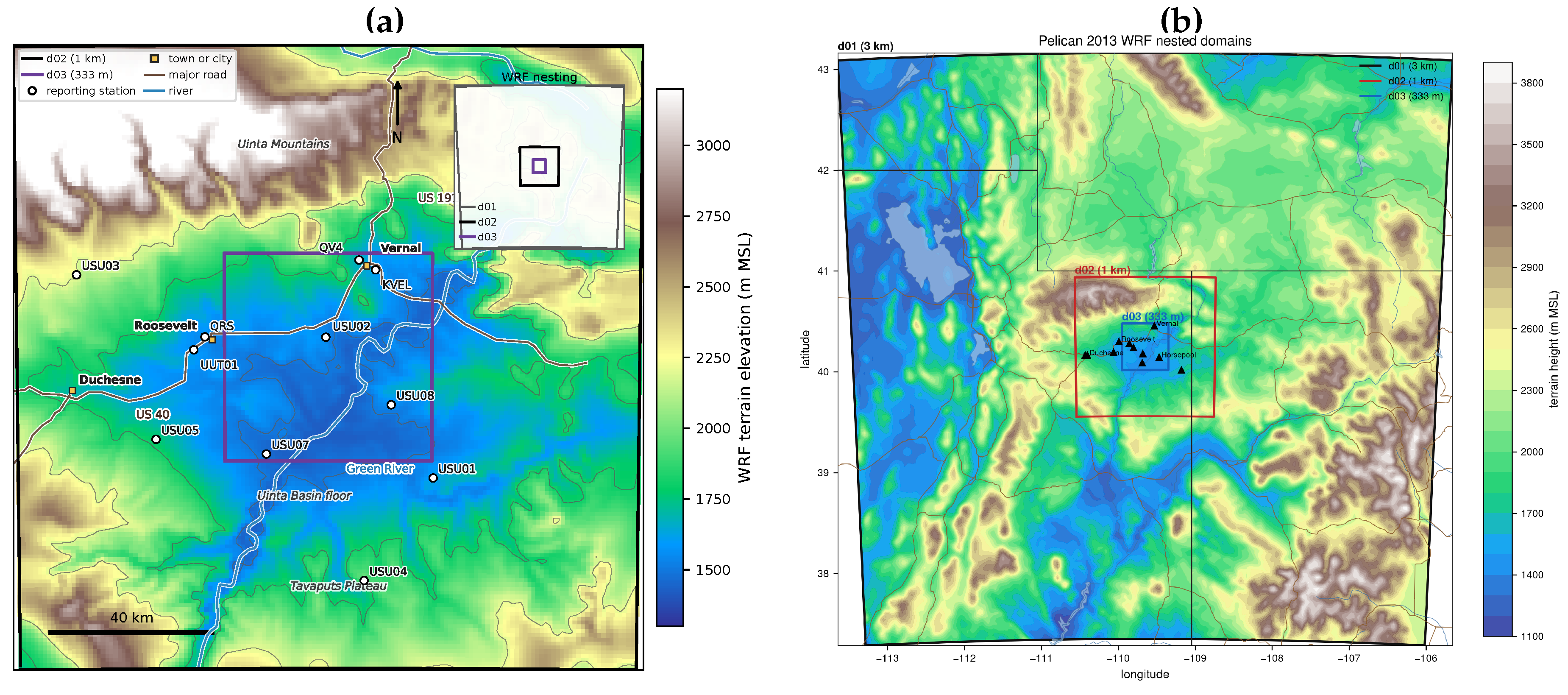
Figure 2.
Observed context for the 2 February 2013 simulation date. (a) NASA GIBS Terra MODIS corrected reflectance, bands 7-2-1, for the 2 February calendar day; snow and ice generally appear cyan, most liquid cloud appears white, and ice cloud may also appear cyan. The nearest centre-covering Terra granule was acquired at 1815–1820 UTC. (b) EPA AQS first maximum value from the daily-summary row at Ouray, Redwash, Roosevelt, Vernal, and Little Mountain, converted from ppm to ppb and plotted by local date without recomputation. All five sites have 59 daily rows; hollow markers identify the seven site-days with less than 75% within-day observation coverage.
Figure 2.
Observed context for the 2 February 2013 simulation date. (a) NASA GIBS Terra MODIS corrected reflectance, bands 7-2-1, for the 2 February calendar day; snow and ice generally appear cyan, most liquid cloud appears white, and ice cloud may also appear cyan. The nearest centre-covering Terra granule was acquired at 1815–1820 UTC. (b) EPA AQS first maximum value from the daily-summary row at Ouray, Redwash, Roosevelt, Vernal, and Little Mountain, converted from ppm to ppb and plotted by local date without recomputation. All five sites have 59 daily rows; hollow markers identify the seven site-days with less than 75% within-day observation coverage.
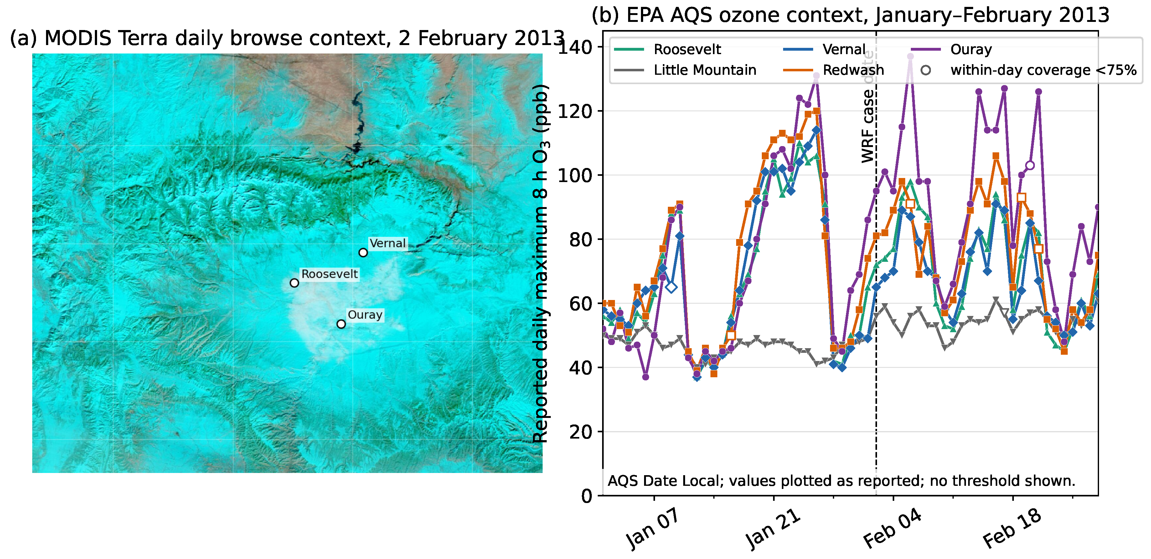
Figure 3.
Observed 2 m-temperature evolution at four elevation-spanning Uinta Basin stations from 31 January through 3 February 2013. Shading indicates approximate local night. The basin-floor site repeatedly separates from the higher sites, and the ordering evolves through the diurnal cycle. The sites establish a recurring spatial surface-temperature pattern but not a colocated vertical profile.
Figure 3.
Observed 2 m-temperature evolution at four elevation-spanning Uinta Basin stations from 31 January through 3 February 2013. Shading indicates approximate local night. The basin-floor site repeatedly separates from the higher sites, and the ordering evolves through the diurnal cycle. The sites establish a recurring spatial surface-temperature pattern but not a colocated vertical profile.
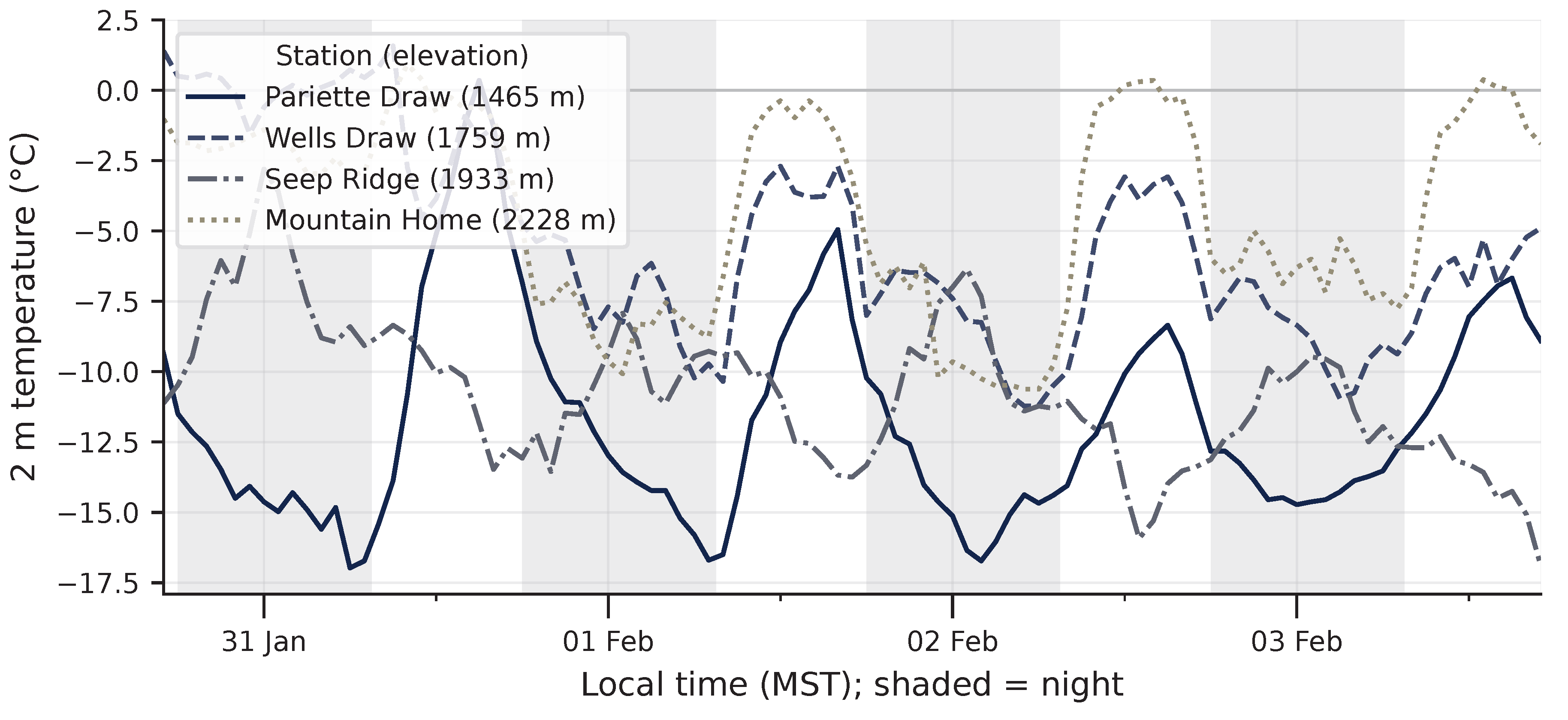
Figure 4.
Mean five-hour effects for the comparisons. Colours and marker shapes identify driving-product, feedback, and interaction contrasts; each row states its differencing direction for quick reference. Whiskers are descriptive block-sensitivity intervals for five dependent hourly medians, not confidence intervals.
Figure 4.
Mean five-hour effects for the comparisons. Colours and marker shapes identify driving-product, feedback, and interaction contrasts; each row states its differencing direction for quick reference. Whiskers are descriptive block-sensitivity intervals for five dependent hourly medians, not confidence intervals.
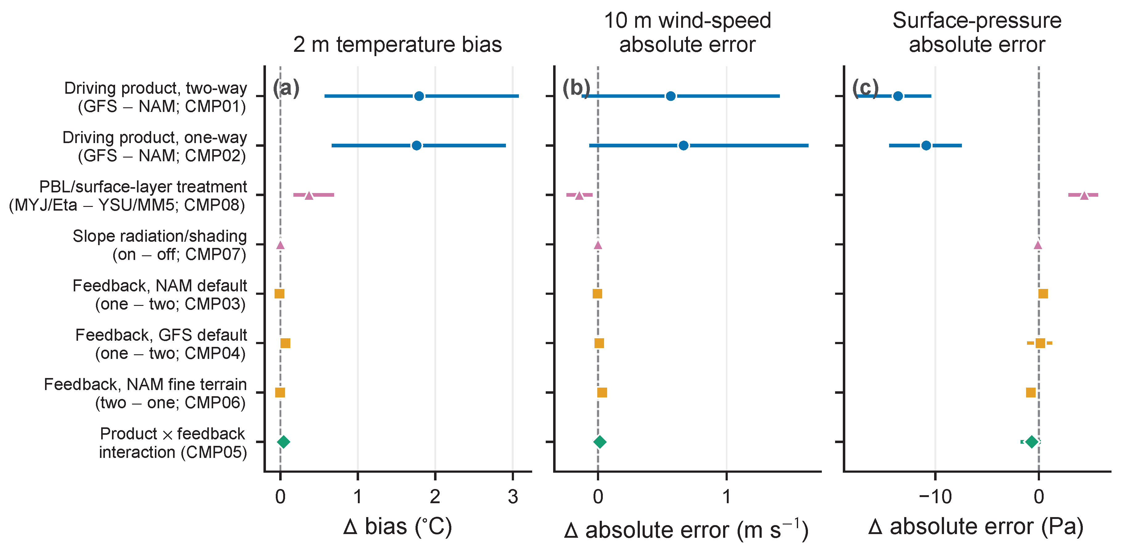
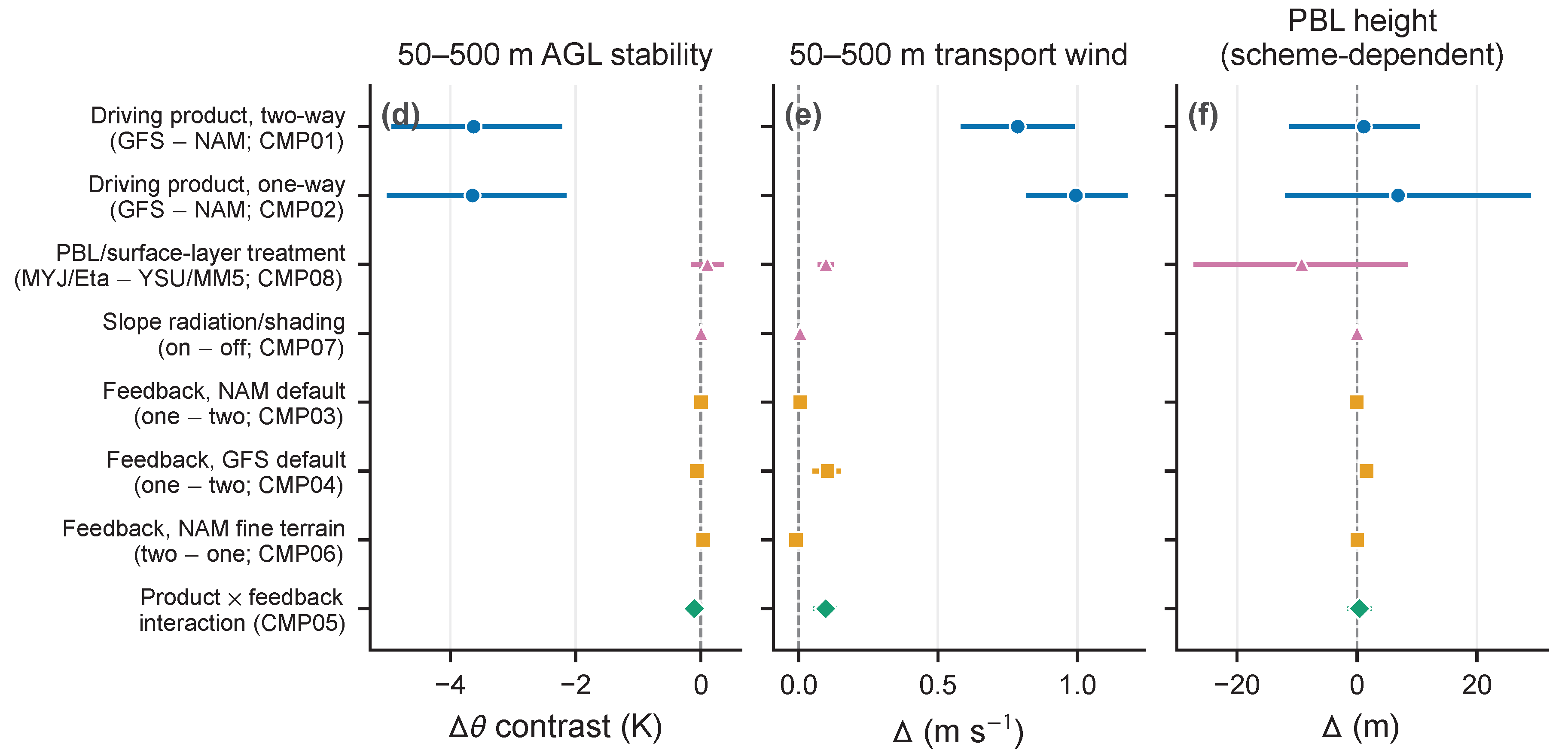
Figure 5.
Station-column medians and interquartile ranges for 50–500 m AGL potential-temperature stability and fixed-layer transport wind over the matched window. Solid lines denote two-way feedback and dashed lines denote one-way feedback. The lower-layer GFS–NAM separation recurs under both feedback modes: GFS is 3.6 K less stable and 0.8–1.0 m s−1 greater in transport wind over the five-hour summary.
Figure 5.
Station-column medians and interquartile ranges for 50–500 m AGL potential-temperature stability and fixed-layer transport wind over the matched window. Solid lines denote two-way feedback and dashed lines denote one-way feedback. The lower-layer GFS–NAM separation recurs under both feedback modes: GFS is 3.6 K less stable and 0.8–1.0 m s−1 greater in transport wind over the five-hour summary.
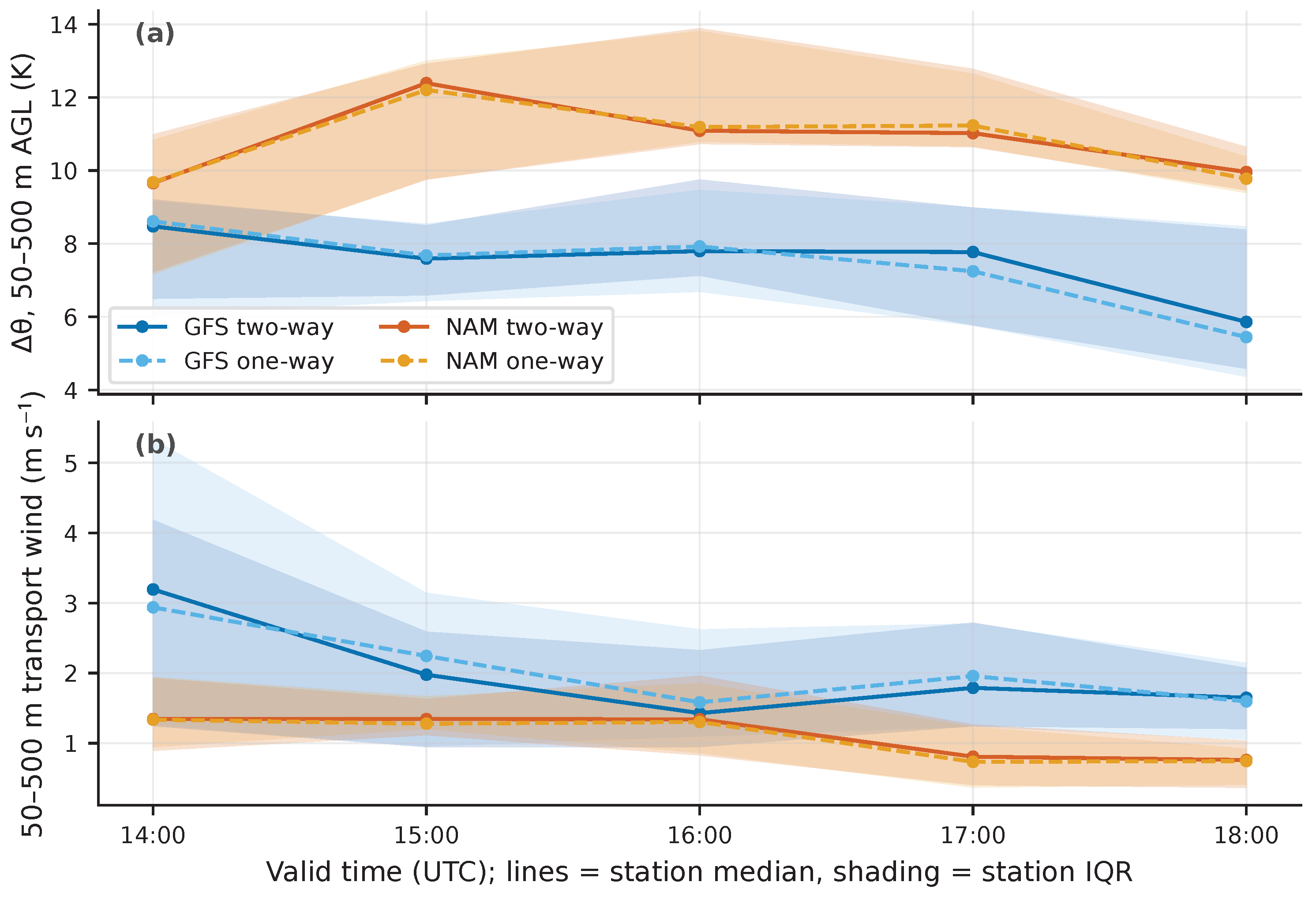
Figure 6.
Observed and modelled Mountain Home-minus-Pariette Draw surface potential-temperature contrast from 1400 to 1800 UTC on 2 February 2013. The modelled series are X6 (GFS two-way) and X5 (NAM two-way) sampled on d02, and all three series contain the same five retained hourly values after the first two forecast hours were excluded.
Figure 6.
Observed and modelled Mountain Home-minus-Pariette Draw surface potential-temperature contrast from 1400 to 1800 UTC on 2 February 2013. The modelled series are X6 (GFS two-way) and X5 (NAM two-way) sampled on d02, and all three series contain the same five retained hourly values after the first two forecast hours were excluded.
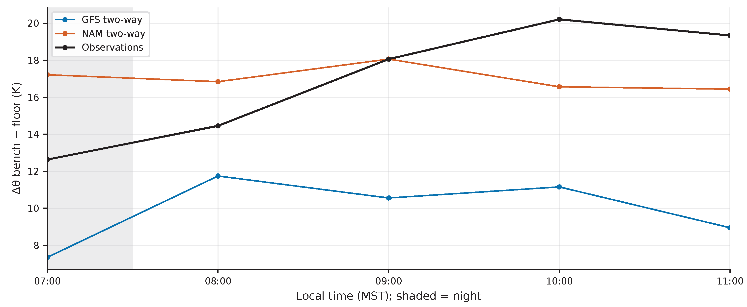
Figure 7.
Heat-deficit trajectories for the four default-terrain matrix members and seven-definition sensitivity envelopes for the two GFS-minus-NAM pairs. The 1300 UTC values orientate the trajectories but are excluded from every reported criterion and effect. GFS retains a smaller deficit throughout, but the deficit does not decline faster in either GFS member.
Figure 7.
Heat-deficit trajectories for the four default-terrain matrix members and seven-definition sensitivity envelopes for the two GFS-minus-NAM pairs. The 1300 UTC values orientate the trajectories but are excluded from every reported criterion and effect. GFS retains a smaller deficit throughout, but the deficit does not decline faster in either GFS member.
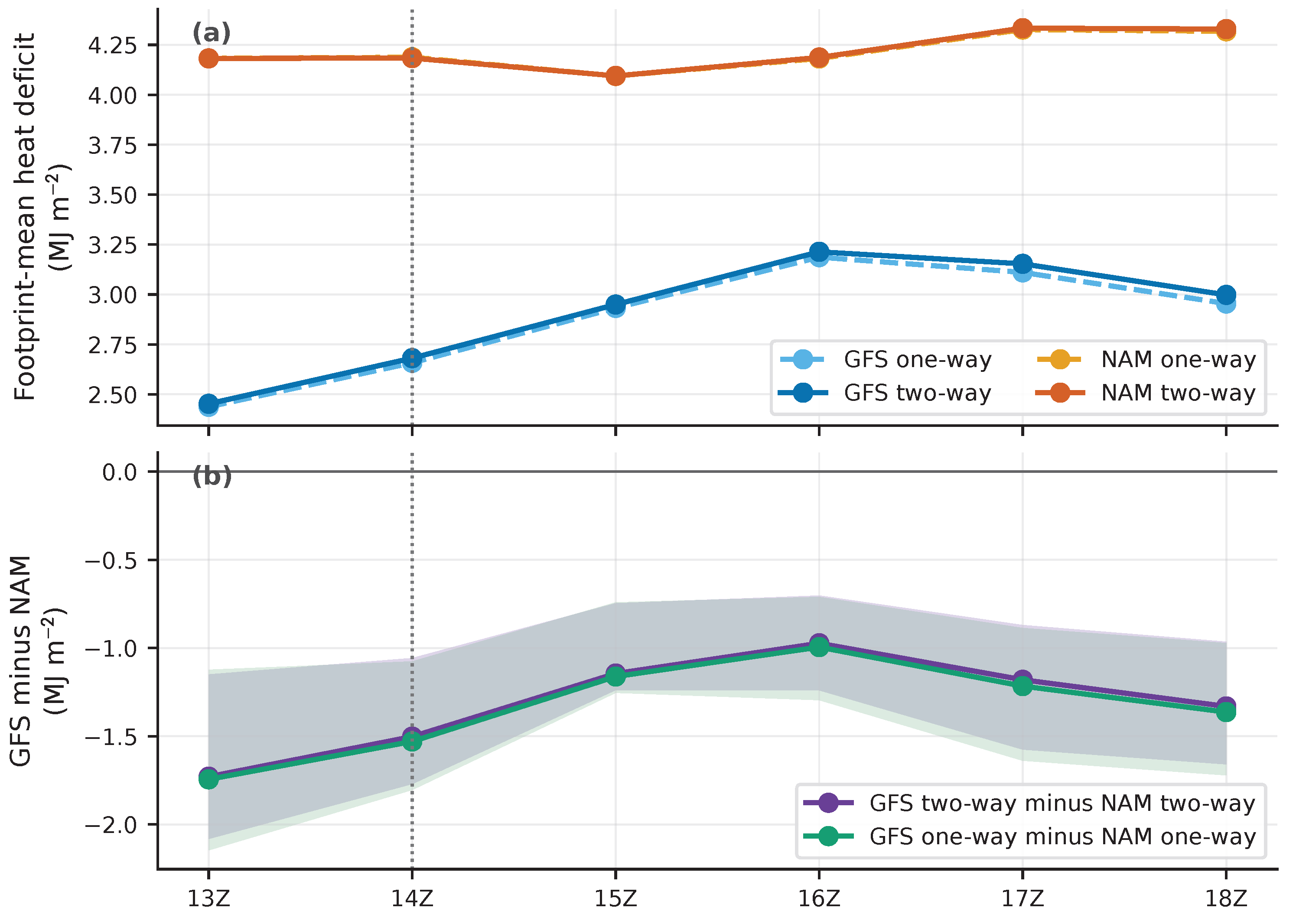
Figure 8.
Diagnostic response to the terrain-resolution experiments at 1600 UTC, calculated as X0 minus X4 (fine 3-arc-second minus coarse 5-arc-minute source). (a) The basin-wide d02 and (b) inner-basin d03 top-down heat-deficit maps share a fixed MJ m−2 scale. (c) The north–south and (d) west–east d03 lower-atmosphere potential-temperature sections share a fixed K scale and the 2200 m crest reference.
Figure 8.
Diagnostic response to the terrain-resolution experiments at 1600 UTC, calculated as X0 minus X4 (fine 3-arc-second minus coarse 5-arc-minute source). (a) The basin-wide d02 and (b) inner-basin d03 top-down heat-deficit maps share a fixed MJ m−2 scale. (c) The north–south and (d) west–east d03 lower-atmosphere potential-temperature sections share a fixed K scale and the 2200 m crest reference.
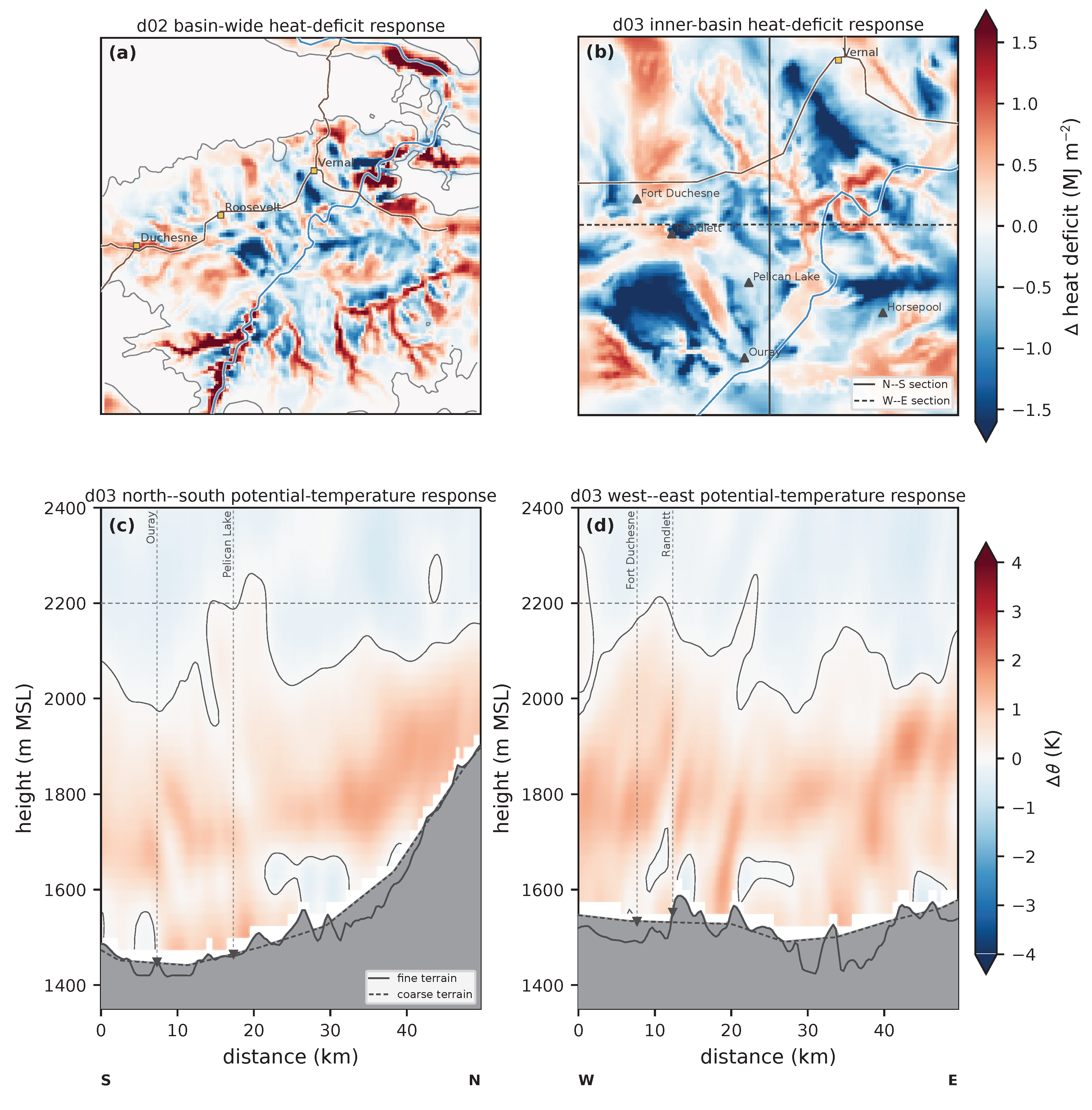
Figure 9.
Model-only d03 potential-temperature profiles at Horsepool for X6 (GFS two-way) and X5 (NAM two-way). (a) The 1200 UTC initialised states and (b) the 1300 UTC one-hour forecasts use identical axes. Grey shading marks levels below the local model terrain, and the dashed 2200 m line is the fixed heat-deficit crest reference rather than an observed cold-pool top
Figure 9.
Model-only d03 potential-temperature profiles at Horsepool for X6 (GFS two-way) and X5 (NAM two-way). (a) The 1200 UTC initialised states and (b) the 1300 UTC one-hour forecasts use identical axes. Grey shading marks levels below the local model terrain, and the dashed 2200 m line is the fixed heat-deficit crest reference rather than an observed cold-pool top
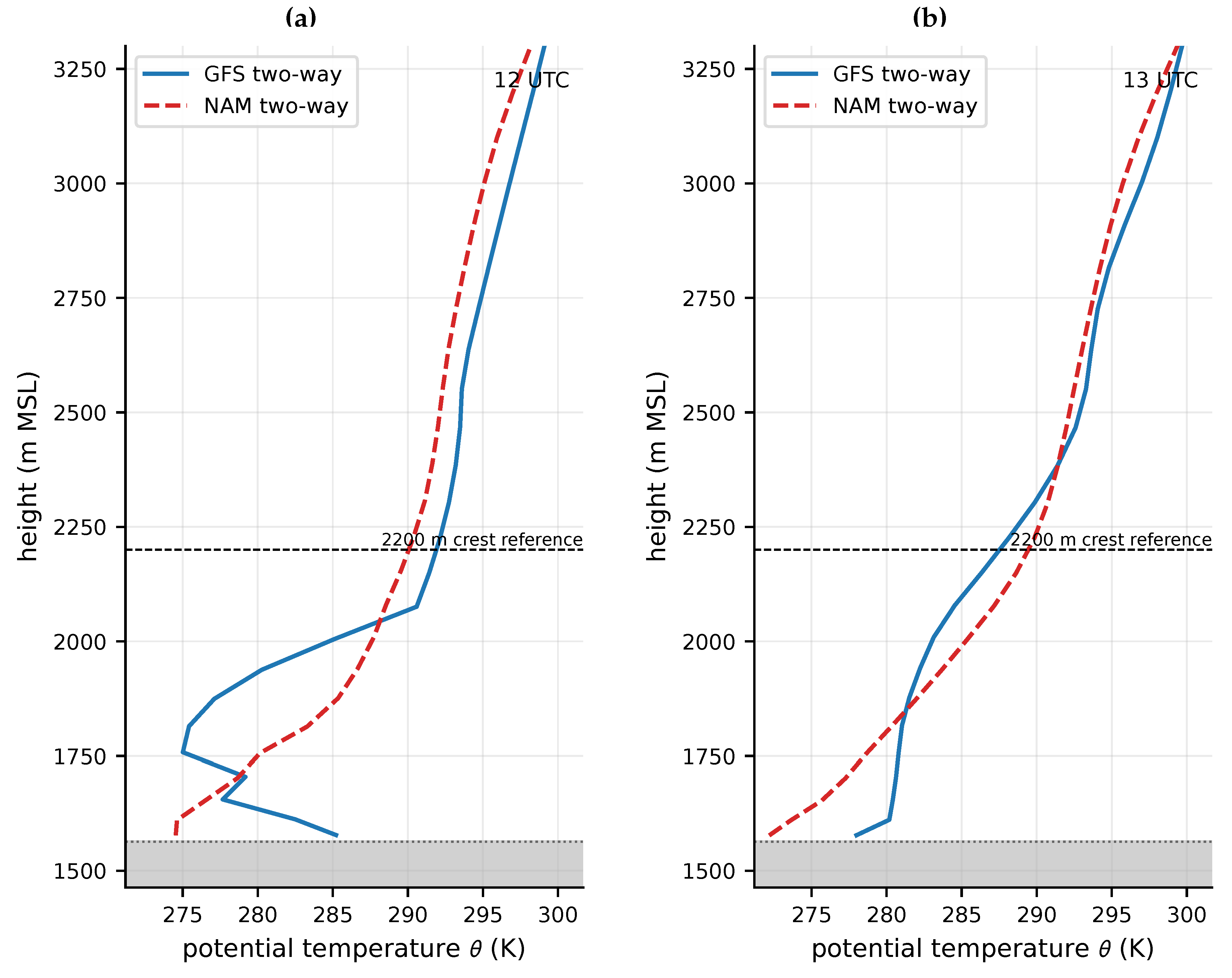
Table 1.
The simulation inventory. Every run uses WRF 4.8.0, three nests at 3/1/0.333 km with 75 levels, Thompson microphysics, RRTMG radiation, and Noah land surface unless stated. “Fine terrain” is the custom 3-arc-second source, “default terrain” is 30-arc-second class, and “coarse terrain” is the 5-arc-minute GMTED2010 source
Table 1.
The simulation inventory. Every run uses WRF 4.8.0, three nests at 3/1/0.333 km with 75 levels, Thompson microphysics, RRTMG radiation, and Noah land surface unless stated. “Fine terrain” is the custom 3-arc-second source, “default terrain” is 30-arc-second class, and “coarse terrain” is the 5-arc-minute GMTED2010 source
| Code | Product, feedback | Configuration and role |
|---|---|---|
| X0 | NAM, one-way | fine-terrain YSU/MM5 control for X1, X3, X4, and X9 |
| X1 | NAM, one-way | X0 plus slope radiation and shading |
| X2 | NAM, one-way | X1 with MYJ/Eta instead of YSU/MM5 |
| X3 | NAM, one-way | default-terrain reference configuration |
| X4 | NAM, one-way | deliberately coarse 5-arc-minute terrain |
| X5 | NAM, two-way | default terrain |
| X6 | GFS, two-way | default terrain |
| X7 | NAM, two-way | 1 km inner grid and 24 h integration; design context only |
| X8 | NAM, one-way | four domains to 111 m and 50 levels; design context only |
| X9 | NAM, two-way | X0 with two-way feedback |
| X10 | GFS, one-way | default terrain |
Table 2.
Controlled contrasts referenced in this study, their differencing orientation, and their scientific use.
Table 2.
Controlled contrasts referenced in this study, their differencing orientation, and their scientific use.
| Operation | Isolated lever | Use in this study |
|---|---|---|
| X6 − X5 | driving product (two-way) | primary controlled contrast |
| X10 − X3 | driving product (one-way) | primary controlled contrast |
| X2 − X1 | PBL and surface-layer scheme | secondary controlled contrast |
| X1 − X0 | slope radiation and shading | spatial diagnostic with an archive limitation |
| X3 − X5 | feedback, NAM, default terrain | secondary robustness contrast |
| X10 − X6 | feedback, GFS, default terrain | secondary robustness contrast |
| X9 − X0 | feedback, NAM, fine terrain | secondary robustness contrast |
| (X10−X6)−(X3−X5) | driving-product-by-feedback interaction | secondary interaction contrast |
| X3 − X0 | terrain source, default vs fine | bounded terrain response; no source ranking |
| X3 − X4 | terrain source, default vs coarse | bounded terrain response; no source ranking |
| X0 − X4 | terrain source, fine vs coarse | bounded terrain response; no source ranking |
Disclaimer/Publisher’s Note: The statements, opinions and data contained in all publications are solely those of the individual author(s) and contributor(s) and not of MDPI and/or the editor(s). MDPI and/or the editor(s) disclaim responsibility for any injury to people or property resulting from any ideas, methods, instructions or products referred to in the content. |
© 2026 by the authors. Licensee MDPI, Basel, Switzerland. This article is an open access article distributed under the terms and conditions of the Creative Commons Attribution (CC BY) license (http://creativecommons.org/licenses/by/4.0/).
Copyright: This open access article is published under a Creative Commons CC BY 4.0 license, which permit the free download, distribution, and reuse, provided that the author and preprint are cited in any reuse.