

Submitted:
16 July 2026
Posted:
17 July 2026
You are already at the latest version
Abstract
Neural implicit surface representations have been proven to be an effective manner to express 3d shapes, but it still has some artificial defects of lacking geometric or topological accuracy for complex shape regions. To solve this issue, a coarse-to-fine training strategy and a piecewise implicit surface reconstruction network are presented to effectively capture the subtle geometric structures from input point cloud shapes. The encoder of our network is designed with piecewise patch feature channel and multi-scale feature aggregation to effectively capture fine shape structures as well as to avoid being affected by non-uniform point cloud distribution. For the decoder of our network, a novel strategy of surface accuracy optimization (SAO) is introduced to progressively learn the underlying implicit surfaces, which can control its accuracy of surface learning under a predefined tolerance parameter whilst further recovering local geometry details in a coarse-to-fine learning manner. Extensive experiments demonstrate that our network design and training method can effectively reconstruct the global shape of the underlying point cloud data while maintaining its fine surface details and also suppressing the artefacts. Compared to the traditional methods, our proposed network has always shown its competitive performance on both IoU and CD errors. Such as, our reconstruction results on the ShapeNet dataset are improved by an average of 7.11%, 20.15%, and 1.99% in terms of IoU index, comparing with DeepSDF, ONet, and CONet methods, respectively; and also reduced by an average of 76.28%, 83.33%, and 36.97% in terms of CD error, respectively.
Keywords:
surface reconstruction
; point cloud
; neural implicit surface
; multi-scale feature aggregation
; surface accuracy optimization (SAO)
1. Introduction
Surface reconstruction is a fundamental and challenging task in the area of computer graphics or 3d computer vision, which can be beneficial to the fields of computer-aided design, scene understanding, visual navigation and robotics [1,2,3]. With the popularity of 3d scanners and depth cameras, discrete point cloud scanning data have been widely exploited as a dominant representation of complex 3d shapes or indoor scenes because of its easy acquisition and also need not require maintenance of complex topological connectivity [4,5,6,7,8]. One of the key issues is how to efficiently reconstruct a discrete surface from sparse point cloud data. Traditional geometry-based reconstruction approaches, such as Poisson surface reconstruction [9] and radial basis function based reconstruction [10] always require a high quality of model data, which will lead to significant degradation of reconstruction performance when the input data contains a lot of model noise [11,12]. Therefore, implicit reconstruction methods based on deep learning are currently gaining widespread attention [13,14,15,16], which can always be less affected by model noise and also have higher reconstruction performance.
Owing to its effectiveness in representing surfaces with arbitrarily complex topology by learning a continuous implicit field [17,18], a deep neural network based scheme can directly learn the signed distance fields (SDFs) or binary occupancy fields (BOFs) from raw point cloud data and always has satisfied generalization performance. The traditional DeepSDF method [19] learned a continuous signed distance function to represent a category of shapes via an auto-decoder, which can optimize the latent vectors and decoder weights through network back-propagation. The decoder thus can decode these latent vectors to obtain signed distance values of sampling points. The occupancy network (ONet) [20] employed the PointNet encoder [21] to encode the whole input of point cloud data thus to extract its latent feature, and then adopted a decoder to get the occupancy values of each query sampling point. Jin et al.[22] presented a neural implicit representation MuSic-UDF to leverage multi-scale dynamic grids for high-fidelity and flexible surface reconstruction from raw point clouds with arbitrary typologies. These traditional approaches essentially use deep neural networks to learn the overall shape structures but without taking into account the effective representation and learning of local shape details, thus leading to some artificial defects. Due to the voxel representation of point cloud data, Peng et al. [23] presented a convolutional occupancy network (CONet) to perform the convolutional operation on voxel grids for feature learning. Ma et al. [24] proposed Neural-Pull to pull query 3D locations to their closest points on the underlying surface using the predicted SDFs and also the gradient at the query locations. Due to its effectiveness of surface reconstruction from discrete point sets by using implicit moving least-squares (IMLS) algorithm, Liu et al. [25] incorporated IMLS surface generation into deep neural networks for inheriting both the flexibility of point sets and the high-quality of implicit surfaces. Wang et al. [26] introduced a dual octree graph network to learn adaptive volumetric shape representation for 3d shape reconstruction, which employed an encoder-decoder structure to learn feature volume based on the graph convolutions over the dual graph of octree nodes. Ma et al. [27] proposed an OSP method to reconstruct accurate surfaces from sparse point clouds with an on-surface prior, which can learn the SDFs via projecting queries onto the surface represented by a discrete point cloud data. By fusing data from multiple features, Le et al. [28] devised a multifeature data fusion model (MfDFM) that enhances measurement data with high-frequency geometric information to achieve highly accurate surface reconstruction. Chu et al. [29] introduced a diffusion-based generative 3d shape completion method by casting shape completion as a generative task conditioned on the incomplete shape. Ren et al. [30] employed a hierarchical voxel latent diffusion model XCube to generate progressively the higher resolution grids in a coarse-to-fine manner. Yin and Lv [31] presented a self-tuned two-stage framework for point cloud reconstruction, which combines a parameter-free denoising module (TPDn) for noise or outliers removal and thus upsampled by PU-Net to recover fine-grained geometry. By integrating a divide-and-conquer strategy into SDF-based reconstruction, Yang et al. [32] proposed a scalable and high-quality neural implicit representation for 3d scene reconstruction. Based on RGB-D inputs, Jiang et al. [33] presented a radiance field rendering method for indoor scenes reconstruction without pre-computed camera poses. Cao et al. [34] introduced PointAMaLR to enhance feature representation and processing accuracy through attention-guided multi-scale local reconstruction. However, these methods always require voxelization of the whole 3d embedding space, resulting in an exponential increase in the amount of input voxel data and the size of network parameters. So, it is difficult to reconstruct high-resolution 3d complex shapes due to its heavy network training and significant memory demands.
Based on a multi-scale neighboring point feature aggregation module, our presented network efficiently and robustly learns input point cloud features. Moreover, through a surface accuracy optimization (SAO) strategy, the proposed novel piecewise implicit surface reconstruction network progressively learns the implicit surface while controlling its accuracy under a predefined tolerance parameter—starting with coarse overall shapes and advancing in a coarse-to-fine manner to capture increasingly fine local geometric details (see Figure 1). The main contributions of this work can be summarized as follows:
- A piecewise surface reconstruction scheme is presented for implicit surface learning, which can effectively train the local signed distance field of point cloud shapes.
- A multi-scale neighbouring point feature aggregation module is introduced to effectively extract the local features of sampling points, and a decoder is designed that adopts a fully connected residual feature decoding for effectively learning the context information of surface patches.
- Owing to the SAO strategy, the accuracy of implicit surface learning can be controlled by a tolerance parameter, and thus can reconstruct local geometry details of point cloud data progressively in a coarse-to-fine manner.
2. Methods
Owing to the SAO strategy, our proposed network takes discrete point cloud data as input directly and trains the local signed distance field of shape patches. The overall network framework is shown in Figure 2.
The proposed reconstruction network can be divided into the following steps:
- A farthest point sampling algorithm [35] is used to obtain the initial centre and radius of the spherical neighbourhood points to generate the initial surface patches. Then the offset of each sample point within each patch relative to its centre can be calculated separately as the relative coordinates, where the discrete points located in the overlap regions may have several relative coordinates.
- In the network coding stage, two neighbouring point feature aggregation modules of different scales are employed to encode the relative coordinate of each sample point into a 256-dimensional latent vector, thus extracting the feature information of their adjacent sampling points. The first module aggregates 8 neighbouring points around each sample point and the other one is 16. Then the multi-scale features of sampling points can be obtained by stitching these feature information introduced by two modules together, and the corresponding latent vectors of sampling points can be obtained by 4-layer MLP perceptron . These latent vectors of sampling points located on each surface patch can be maximized to characterize the latent features of the surface patch.
- In the network decoding stage, according to the surface optimization strategy, a tolerance parameter is introduced to control the reconstruction accuracy of our network learning. At the beginning of network training, only a shallow network is adopted and the number of network layers can be gradually increased as the number of training rounds. During network learning, the relative coordinates and their corresponding latent features of surface patches will be input to the network decoder to obtain the signed distances of the relative positions of each sampling point. The signed distances of the relative positions of sampling points located in the overlapping regions of different surface patches are weighted and summed to obtain the signed distances of sampling points.
- Based on the Marching Cube algorithm [36], we can extract the zero iso-surface of the signed distance fields to obtain a final 3d mesh model.
2.1. Surface Accuracy Optimization Strategy
Inspired by the human learning mechanism, organizing the tasks for shape feature learning in a simple-to-complex manner can effectively improve the reconstruction performance of our network [37]. In this paper, we adopt a supervised learning strategy to efficiently learn the implicit signed distance field, making the predicted SDF values of sampled points as close as possible to their true SDF values. Considering its effectiveness of supervision with the true SDF values, our proposed reconstruction network will optimize the surface accuracy-based strategy to better learn the local features of point cloud shapes. Specifically, instead of strictly requiring the reconstruction network to estimate SDF values as close as possible to the true SDF values, the accuracy of the learned surface is controlled by an upper tolerance parameter for surface reconstruction error, which allows the network to estimate the underlying shapes with small errors, i.e., the estimated SDF values with errors smaller than are considered to be correct.
For our experiments, start with the relatively large parameter which can focus on the global structure recovery of point cloud shape. Then, gradually lower will expose more fine details of the shape until it drops to . As shown in Figure 3, there is an error region of thickness near the exact surface of the point cloud shape, and the goal of the reconstruction network is to learn and reconstruct shape structures located in this local region. At the beginning of network training, a relatively large value of is set to allow the network to learn relatively smooth and coarse surfaces in this local region. The value of is gradually reduced to expose and learn more fine shape details as the number of training rounds increases, and eventually, the value of is set to to predict the exact reconstructed shape. So, the loss function for surface reconstruction can be designed as follows,
where is the set of sampled points, means the estimated SDF value of the sampling point, and is the corresponding true SDF value of the sampled point.
2.2. Calculation of Signed Distance Values for Sampling Points
For effectively learning the local shape features using a piecewise surface manner, the input discrete point cloud data is divided into surface patches, and the discrete point cloud within each patch is regarded as a local region where the neighbouring information of the surface patch can be represented as a spherical neighbourhood with the patch centre at and the radius of r. Before encoding the input 3d point cloud data, the initial surface patch needs to be generated efficiently so that each surface patch will contain the sampling points as completely and uniformly as possible. Specifically, the input point cloud is first sampled using the farthest point sampling algorithm [35] to obtain the representative point cloud , (where K is the number of sampling points located in the representative point cloud and is taken as 30 for our experiments). The algorithm is performed as follows: firstly, we select a random seed point from the input point cloud data and add it to , then we calculate the Euclidean distance between the seed point and the remaining input sampling points. Secondly, we select the farthest sampling point to be added to , and so on until the number of sampling points included in is K; and the 3d coordinates of each sampling point of are then selected as the centre of each surface patch, i.e.
Furthermore, to determine the radius of each surface patch, we select a random sampling point from the input point cloud data and calculate the Euclidean distance between all sampling points in and find the closest sampling point , which we can mark as a reference point for sampling point . And so on until all the input sampling points are marked as reference points, and thus we calculate the radius of each surface patch as follows,
where indicates all the reference points of sampling point .
To effectively learn the local feature differences of sampling points, instead of taking the original coordinates of sampling points as the input of the encoder, here we employ the relative coordinates of sampling points, that is, the offset of each sample point within each patch relative to its centre respectively, where the discrete points located in the overlap regions may have several relative coordinates. Then, as a pre-processing step before point cloud encoding, the weights of sampling points in each surface patch can be determined according to their Euclidean distances between sampling points and the centre of the surface patch as follows,
Here means the weight of sampling point as to the i-th surface patch . If the sampling point is not located within the i-th surface patch, the weight is zero, otherwise the smaller the distance between and centre of i-th surface patch , the larger the weight. Here is taken as .
Further, to extract and aggregate local information of adjacent sampling points, we encode the relative coordinates of each sample point in our network encoder and generate a 256-dimensional latent vector by using the neighbouring point aggregation strategy. Meanwhile, the latent vector of the surface patch can be created as the maximum of the latent vectors of sampling points located in this surface patch. Finally, during the network decoding step, a multi-layer fully connected residual feature decoding module is employed to obtain the signed distance values of each sample point. It should be noted that for sampling points that are located in the overlap regions of several adjacent patches, the signed distance of sampling points could be weighted and the sum of the signed distance values of adjacent patches as follows,
2.3. Encoder via Multi-Scale Neighboring Point Feature Aggregation
For point cloud surface reconstruction, due to the inconsistency of sampling density in different regions of point cloud shape, capturing the point feature information only using a single scale neighbouring points may not be able to learn the local structure of the underlying 3d shapes due to its sparse sampling points in that region. To solve this issue, we adopted the neighbouring point feature aggregation module [38] to fully extract the multi-scale point feature information during the network learning, which can better capture the local shape structure of the underlying point cloud shape.
As shown in Figure 4, taking the 3d coordinates of sampling points as the input of network encoder, and the dimensional point features are first obtained by using a 2-layer perceptron ; then, the multi-scale point features can be extracted by two different scales of the neighbouring point aggregation module and thus stitched then together. As shown in Figure 4, for each neighborhing point feature aggregation module, the local point feature information is firstly extracted by two branches: the first branch aggregates M neighboring points around each sampling point using k-NN algorithm to obtain dimensional feature matrix ; the second branch expands the local feature information of by a factor M of to obtain the dimensional feature matrix ; then these two feature matrices are subtracted to obtain a dimensional feature matrix ; and the feature matrix and are then concatenated to obtain the dimensional feature matrix, and finally the maximum pooling operation is performed on the second dimension of feature matrix to obtain the dimensional neighbouring feature aggregation information of point cloud data. The second point feature aggregation module also performs the above neighbouring point feature aggregation step to form a dimensional neighbourhood feature aggregation information of the point cloud. We can thus stitch these two single-scale point features from the above two branches using concat operation to obtain dimensional multi-scale point feature information. Finally, the dimensional encoding results of the neighbouring aggregation features of the whole point cloud shape can be obtained using a stacking 4-layer perceptron . In our experiments, these two different scales are set to 8 and 16 respectively, which can demonstrate that our strategy of extracting and combining different scale point features is always superior to that of only using a single scale feature encoding in terms of point feature learning.
2.4. Decoder via Surface Accuracy Optimization
During the network encoder encoding the aggregated point features, to effectively estimate the signed distance values of discrete sampling points, both the relative coordinates of sampling points and the aggregated latent features of the corresponding surface patches are adopted as the input to our network decoder, such as shown in Figure 5. Meanwhile, we employ a SAO strategy for our decoder structure. That is, we first use a shallow network to learn a coarse 3d shape with a large value of tolerance parameter at the beginning of network training, and then add more network layers to improve reconstructed surface accuracy while decreasing the value of tolerance parameter as the number of training rounds increases. The number of decoder network layers, the value of discrete interpolation parameter , and the number of training rounds are listed in Table 1.
However, the trained shallow networks may be affected due to the addition of a new untrained layer to our network. Therefore, after adding a new layer, we also give this new layer a weight of , which corresponds to the weight of the old layer of . Here, the weight of can linearly increase from to according to the number of training rounds, so that the original network can smoothly adapt to this new layer. The output of the proposed network in this newly added layer can be calculated as follows.
where denotes the feature matrix of the previous old layer, means the feature matrix of by using the new layer, is the feature matrix of the final network output at this new layer, is the current number of training rounds. In addition, by considering the issue of network degradation due to the large number of decoder layers, we also add the residual network structure [39] to the shallow part of our decoder to improve the network performance. As shown in Figure 5, the shallow network of the decoder includes four fully-connected residual feature decoding modules. Specifically, let the input feature matrix of the module is , and denote the output of the 1-st, 2-nd, 3-th fully-connected layer respectively, and means the weight of the neurons including in fully-connected layer, then the output of each network layer of the module can be calculated as follows,
Here, denotes the ReLU activation function. The final output of the module can be expressed as follows,
where + denotes matrix summation. It should be mentioned that the information loss can be effectively reduced during feature propagation by adding the residual structure, which can enhance the gradient propagation during network training and also improve the decoder performance of decoding features.
2.5. Loss Function
During our task of piecewise surface reconstruction, to control the effective generation of surface patches and learning of the shape latent features [40], the following four items of loss functions are considered for the network training.
- : Keeps surface patches of the same object as close to the object surface as possible,where is the set of all sampling points located on the i-th object and B is the number of objects in a training batch during network training. The loss function is only used when the distance between the object surface and the patches is greater than a threshold T. Since we eventually need to extract the zero iso-surface of sampling points, the centres of each surface patch should be as close as possible to the 3d shape for the selection of sampling points thus using the SAO strategy. The introduced threshold T should be taken as a small value, so we choose in our experiments.
- : Makes the sampling points should be located within at least one surface patch,where is the set of all sampling points for ith-objects that do not located in any of surface patches, and means the weight of sampled points sampled from ith-object that located in the jth-patch.
- : Keeps the surface patch as small as possible to prevent significant overlap between different patches,
- : Makes the size of different patches similar to prevent the surface reconstruction only using few large patches,where is the average radius of the surface patch located in the i-th object, the larger the patch radius the larger the value of the loss function, thus can prevent the reconstruction network from generating large surface patches.
Finally, the loss function of our network can be defined as follows,
Here, the weight of is set to to be defined as a benchmark, and thus we can determine the weights of other losses. The other losses are designed so that as many sample points located near the object’s surface as possible are included in the surface patches. So, we always set large weights to the and losses and small weights to and . In our experiments, the weights of this total loss function are selected as , , , and .
3. Experimental Results
The proposed implicit surface reconstruction network has been trained on an NVIDIA RTX 3060 GPU using the PyTorch framework. As a preprocessing step, a total of 200,000 discrete sampling points are sampled from each 3d object. In our experiments, a total of randomly selected sampling points from the point cloud shapes contained in each training batch are chosen as the input to the reconstruction network and their signed distance values can be effectively learned. The presented network is trained with the help of Adam Optimiser. The learning rate is set to , which is halved every 200 round, and the batch size is 2.
3.1. Surface Reconstruction via Our Network
To illustrate the effectiveness of our reconstruction network, we first train and test our network on the public ShapeNet dataset [1], which is a large-scale public 3d shape dataset produced by researchers from Princeton University, Stanford University, and TTIC. We select some typical 3d shapes, such as sofa, chair, airplane, and other categories from the ShapeNet dataset, and 100 models are selected for each object category and trained for 1000 rounds. The surface reconstruction results are shown in Figure 1 and Figure 6. From these experiments, it can be seen that the introduced method can not only completely reconstruct the overall shape of a 3d object, but also effectively reconstruct the local fine structures such as the pillows on the sofa, the foot of the chair, the tail of the airplane, the back of the individual seat, and the lamp holder. In general, the reconstructed model is not only consistent with the real object in terms of overall structure but also reconstructs the complex fine structures of 3d objects and suppresses the artefacts.
Furthermore, to verify its generalization of the proposed reconstruction network, we also experimented on the Famous dataset [41] and used our network to over-fit each point cloud shape. Reconstruction results are shown in Figure 7. These experimental results demonstrate that our method can effectively reconstruct the overall structure of the objects with different shape categories from the ShapeNet dataset [1], which can validate its ability of good generalization.
3.2. Method Comparisons
To illustrate the effectiveness of our presented network, we compared our network with the existing methods and employed the same subset of models selected from the ShapeNet dataset [1] as the network training and test sets. The occupancy network [20] and convolutional occupancy network [23] use the pre-trained models provided by their authors, while the Intersection on Union (IoU) and Chamfer distance (CD) error [22] are adopted as the metrics to evaluate their effectiveness of object reconstruction.
Figure 8 gives the reconstruction results both of our network and other existing methods. As shown in Figure 8, the DeepSDF network [19] and occupancy network [20] can only reconstruct the general overall structure of the underlying point cloud shapes, and there are a lot of man-made artefacts around the reconstructed model, whilst the convolutional occupancy network [23] and our presented network can reconstruct the overall shape of point cloud model accurately (such as motorboat and rifle), and the reconstruction results are significantly better than the above two networks. In terms of shape details, our proposed network can generate fewer man-made artefacts if reconstructing sub-parts with large holes, such as the cabin of a motorboat. The DeepSDF network [19] and the occupancy network [20] always introduce more man-made artefacts, and is also difficult to recover those local fine structures. This is because the global feature learning method only can learn their overall shape, and does not pay enough attention to the local fine shape details, which leads to its difficulty in reconstructing the fine structures of point cloud shapes. Furthermore, compared with the traditional convolutional occupancy network [23], our proposed network can obtain better reconstruction results for fine structures, such as gun barrels, the helm of the ship, the leg of the sofa, and the tail tip of the aircraft, etc, which indicates that our introduced reconstruction network outperforms the traditional convolutional occupancy network [23] in terms of learning local fine structures. Moreover, the reconstruction of shape components (such as the gap between pillows, scope, and body of the gun) always leads to less adhesion between different components, which indicates that our proposed network can suppress reconstruction artefacts better than that of a convolutional occupancy network [23].
Compared with the global feature learning networks, such as DeepSDF network [19] and occupancy network [20], our proposed network can effectively learn local features of the underlying shapes, which can not only provide a completed reconstruction with fewer artefacts but also effectively reconstruct the local fine shape details. Compared to the convolutional occupancy network [23], our presented network can effectively extract the shape features by using multi-scale neighbouring point feature aggregation operation in the encoding stage, and also reduce the loss of feature information during gradient propagation through the residual structure in the decoding stage. Meanwhile, owing to the surface accuracy optimization strategy, our reconstruction network can understand and effectively learn the complex structure information of the underlying shapes, and thus can reconstruct the local shape details in a more fine-grained manner, which validates a better reconstruction performance than that of convolutional occupancy network [23].
Table 2 shows the data statistics for different reconstruction networks on the ShapeNet dataset [1]. The higher the IoU metric and the lower the CD error metric, the closer the reconstruction results are to the ground truth, which gives better reconstruction results. From the data in Table 2, it can be seen that our proposed network and the convolutional occupancy network [23] outperform traditional DeepSDF network [19] and the occupancy network [20] in terms of evaluation metrics, which demonstrate its advantage of local feature learning over global feature learning. Such as, the reconstruction results on the ShapeNet dataset of our network are improved by an average of , , and in terms of IoU index, comparing with DeepSDF, ONet, and CONet methods, respectively; and also reduced by an average of , , and in terms of CD error, respectively. Moreover, our proposed network has the best values in both evaluation metrics and also shows better reconstruction performance.
4. Discussion
To perform an ablation study, here we first construct a baseline network for surface reconstruction that only uses 10 patches without the SAO strategy and also remove the fully connected residual feature decoding module and the multiscale neighbouring point feature aggregation module. Then, we also train our network by using full 30 patches, and adding the SAO optimization strategy, and adding the other modules to our baseline network. For the network training, we select 100 point cloud models of the chair category from the ShapeNet dataset [1]. The quantitative statistics of the reconstruction are shown in Table 3. Experimental results demonstrate that the reconstruction performance of the network gradually increases with the number of surface patches and the addition of different modules. While the number of surface patches is increased from 10 to 30 in the baseline network, the reconstruction performance is significantly improved because a larger number of patches can always learn local fine feature information even in a smaller object region. On the other hand, if the surface accuracy optimization strategy is included in the reconstruction network, it can gradually learn more and more complex structures of point cloud shapes, which can easily understand the point cloud information than that of the direct feature learning and thus achieve better reconstruction performance.
5. Conclusions
Owing to a SAO strategy, we proposed a piecewise implicit surface learning network for surface reconstruction. Taking the point cloud data as direct input, the network adopted a multi-scale neighbouring point feature aggregation module to effectively extract the local feature information of sampling points. Moreover, we introduced a tolerance parameter to control the reconstruction accuracy of the piecewise reconstruction network, that is, only shallow layers are employed at the beginning of the network training, and the number of layers is gradually increased with the number of training rounds, which allows the reconstruction network to learn more and more complex shape feature progressively. Experiments illustrate that our reconstruction network can effectively reconstruct the local fine structures of 3d objects, reducing the incorrect adhesion between model components, and leading to only fewer reconstruction artifacts.
However, to better reconstruct the detailed features of 3d objects, future work could consider how to employ optimization methods such as pre-processing the original point cloud data to aid 3d reconstruction. Meanwhile, the encoder structures may be optimized and improved to speed up the network training whilst better learning the intrinsic features of point cloud shapes.
Author Contributions
Conceptualization, X.Z. and Y.M.; methodology, J.M. and Y.Z. and X.Z.; software, J.M. and Y.Z.; validation, J.M. and X.Z.; formal analysis, J.M.; investigation, J.M. and Y.Z.; resources, X.Z. and Y.M.; data curation, J.M.; writing—original draft preparation, J.M.; writing—review and editing, X.Z. and Y.M.; visualization, Y.Z.; supervision, Y.M.; project administration, X.Z.; funding acquisition, X.Z. and Y.M. All authors have read and agreed to the published version of the manuscript.
Funding
This work was supported by the Zhejiang Provincial Natural Science Foundation of China under Grant No. LZ23F020002, and the Key Laboratory of Artificial Organs and Computational Medicine of Zhejiang Province under Grant No. SZD2025B016.
Data Availability Statement
The datasets tested and/or analyzed during the current study are publicly available benchmark datasets, that is Shapenet Dateset (https://shapenet.org/) and Famous Dataset.
Conflicts of Interest
The authors declare no conflicts of interest.
Abbreviations
The following abbreviations are used in this manuscript:
| SAO | Surface accuracy optimization |
| SDFs | Signed distance fields |
| ONet | Occupancy network |
| CONet | Convolutional occupancy network |
References
- Chang, A.X.; Funkhouser, T.; Guibas, L.; Hanrahan, P.; Huang, Q.; Li, Z.; Savarese, S.; Savva, M.; Song, S.; Su, H.; Xiao, J.; Yi, L.; Yu, F. Shapenet: An information-rich 3d model repository. arXiv 2015, arXiv:151203012. [Google Scholar]
- Jin, T.; Zhuang, J.; Xiao, J.; Xu, N.; Qin, S. Reconstructing floorplans from point clouds using GAN. J. Imaging 2023, 9(2), 39. [Google Scholar] [CrossRef] [PubMed]
- Sun, Y.; Zhang, X.; Miao, Y. A review of point cloud segmentation for understanding 3D indoor scenes. Vis. Intell. 2024, 2(1), 14. [Google Scholar] [CrossRef]
- Miao, Y.; Xiao, C. Geometric processing and shape modeling of 3d point-sampled models; Science Press: Beijing, 2014. [Google Scholar]
- Trujillo-Jiménez, M.A.; Navarro, P.; Pazos, B.; Morales, L.; Ramallo, V.; Paschetta, C.; De Azevedo, S.; Ruderman, A.; Pérez, O.; Delrieux, C.; Gonzalez-José, R. Body2vec: 3D point cloud reconstruction for precise anthropometry with handheld devices. J. Imaging 2020, 6(9), 94. [Google Scholar] [CrossRef] [PubMed]
- Yang, X.; Ji, D.; Li, Y.; Xie, J.; Guo, J.; Guo, Y. EdgeMovingNet: Edge-preserving point cloud reconstruction via joint geometry features. In Proceedings of the IEEE/CVF Conference on Computer Vision and Pattern Recognition (CVPR), Nashville, TN, USA, 2025; pp. 22150–22160. [Google Scholar]
- Tian, S.; Chen, W.; He, W.; Zhao, Q.; Zhang, L. View refinement net: Pluralistic shape completion. Neurocomputing 2026, 672, 132691. [Google Scholar] [CrossRef]
- Hu, Y.; Wu, Y.; Mo, Y.; Wang, J.; Zhang, Y. DAPU: Distribution-aware patch upsampling for point cloud based 3D object detection. Neurocomputing 2026, 670, 132579. [Google Scholar] [CrossRef]
- Kazhdan, M.; Hoppe, H. Screened poisson surface reconstruction. ACM Trans. Graph. 2013, 32(3), Articel No. 29. [Google Scholar] [CrossRef]
- Zeng, Y.; Zhu, Y. Implicit surface reconstruction based on a new interpolation approximation radial basis function. Comput. Aided Geom. Des. 2022, 92, 102062. [Google Scholar] [CrossRef]
- Kazhdan, M.; Chuang, M.; Rusinkiewicz, S.; Hoppe, H. Poisson surface reconstruction with envelope constraints. Comput. Graph. Forum 2020, 39(5), 173–182. [Google Scholar] [CrossRef]
- Kazhdan, M.; Hoppe, H. Distributed poisson surface reconstruction. Comput. Graph. Forum 2023, 42(6), e14925. [Google Scholar] [CrossRef]
- Schirmer, L.; Novello, T.; da Silva, V.; Schardong, G.; Perazzo, D.; Lopes, H.; Gonçalves, N.; Velho, L. Geometric implicit neural representations for signed distance functions. Comput. Graph. 2024, 125, 104085. [Google Scholar] [CrossRef]
- Lyu, X.; Sun, Y.-T.; Huang, Y.-H.; Wu, X.; Yang, Z.; Chen, Y.; Pang, J.; Qi, X. 3DGSR: Implicit surface reconstruction with 3D gaussian splatting. ACM Trans. Graph. 2024, 43(6), Articel No. 198. [Google Scholar] [CrossRef]
- Zhang, X.; Yu, R.; Ren, S. Neural implicit representations for multi-view surface reconstruction: A survey. IEEE Trans. Vis. Comput. Graph. 2025, 31(10), 9444–963. [Google Scholar] [CrossRef] [PubMed]
- Zhu, C.; Liu, X.; Xu, K.; Yi, R. A survey on 3D editing based on NeRF and 3DGS. Front. Comput. Sci. 2026, 20(4), 2004701. [Google Scholar]
- Han, L.; Zhang, X.; Song, H.; Shi, K.; Liu, Y.S.; Han, Z. SparseRecon: Neural implicit surface reconstruction from sparse views with feature and depth consistencies. In Proceedings of the IEEE/CVF International Conference on Computer Vision (ICCV), Honolulu, HI, USA, 2025; pp. 28514–28524. [Google Scholar]
- Patel, A.; Laga, H.; Sharma, O. Normal-guided detail-preserving neural implicit function for high-fidelity 3D surface reconstruction. In Proceedings of the ACM on Computer Graphics and Interactive Techniques, Association for Computing Machinery, New York, NY, 2025; 8, p. Article No. 12. [Google Scholar]
- Park, J.J.; Florence, P.; Straub, J.; Newcombe, R.; Lovegrove, S. Deepsdf: Learning continuous signed distance functions for shape representation. In Proceedings of the IEEE/CVF Computer Vision and Pattern Recognition (CVPR), Long Beach, CA, USA, 2019; pp. 165–174. [Google Scholar]
- Mescheder, L.; Oechsle, M.; Niemeyer, M.; Nowozin, S.; Geiger, A. Occupancy networks: Learning 3d reconstruction in function space. In Proceedings of the IEEE/CVF Computer Vision and Pattern Recognition (CVPR), Long Beach, CA, USA, 2019; pp. 4460–4470. [Google Scholar]
- Qi, C.R.; Su, H.; Mo, K.; Guibas, L.J. Pointnet: Deep learning on point sets for 3d classification and segmentation. In Proceedings of the IEEE/CVF Computer Vision and Pattern Recognition (CVPR), Honolulu, HI, USA, 2017; pp. 652–660. [Google Scholar]
- Jin, C.; Wu, T.; Liu, Y.S.; Zhou, J. MuSic-UDF: Learning multi-scale dynamic grid representation for high-fidelity surface reconstruction from point clouds. Comput. Graph. 2024, 124, 104081. [Google Scholar] [CrossRef]
- Peng, S.; Niemeyer, M.; Mescheder, L.; Pollefeys, M.; Geiger, A. Convolutional occupancy networks. In Proceedings of the European Conference on Computer Vision (ECCV), Glasgow, UK, 2020; pp. 523–540. [Google Scholar]
- Ma, B.; Han, Z.; Liu, Y.-S.; Zwicker, M. Neural-Pull: Learning signed distance function from point clouds by learning to pull space onto surface. Proc. 38th Int. Conf. Mach. Learn. 2021, 139, 7246–7257. [Google Scholar]
- Liu, S.L.; Guo, H.X.; Pan, H.; Wang, P.S.; Tong, X.; Liu, Y. Deep implicit moving least-squares functions for 3D reconstruction. In Proceedings of the IEEE/CVF Conference on Computer Vision and Pattern Recognition (CVPR), Nashville, TN, USA, 2021; pp. 1788–1797. [Google Scholar]
- Wang, P.S.; Liu, Y.; Tong, X. Dual octree graph networks for learning adaptive volumetric shape representations. ACM Trans. Graph. 2022, 41(4), Article No. 103. [Google Scholar] [CrossRef]
- Ma, B.; Liu, Y.-S.; Han, Z. Reconstructing surfaces for sparse point clouds with on-surface priors. Proceedings of IEEE/CVF Conference on Computer Vision and Pattern Recognition (CVPR), New Orleans, LA, USA, 2022; pp. 6305–6315. [Google Scholar]
- Le, X.; Pang, D.; Wang, Y.; Chen, C.; Guan, X. Surface reconstruction using geometric features and machining process. IEEE Trans. Instrum. Meas. 2024, 73, 1–10. [Google Scholar] [CrossRef]
- Chu, R.; Xie, E.; Mo, S.; Li, Z.; Nießner, M.; Fu, C.W.; Jia, J. Diffcomplete: Diffusion-based generative 3d shape completion. Advances in Neural Information Processing Systems (NeuIPS), Vancouver, BC, Canada, 2024; Article No. 36. [Google Scholar]
- Ren, X.; Huang, J.; Zeng, X.; Museth, K.; Fidler, S.; Williams, F. Xcube: Large-scale 3d generative modeling using sparse voxel hierarchies. In Proceedings of the IEEE/CVF conference on Computer Vision and Pattern Recognition (CVPR), Seattle, WA, USA, 2024; pp. 4209–4219. [Google Scholar]
- Ying, Z.; Lv, D. Self-tuned two-stage point cloud reconstruction framework combining TPDn and PU-net. J. Imaging 2025, 11(11), 396. [Google Scholar] [CrossRef] [PubMed]
- Yang, L.; Deng, B.; Zhang, J. Scalable and high-quality neural implicit representation for 3D reconstruction. IEEE Trans. Vis. Comput. Graph. 2025, 31(10), 6751–6766. [Google Scholar] [CrossRef] [PubMed]
- Jiang, W.; Liu, Y.; Ouyang, M.; Zhang, X. MT-NeRF: Neural implicit representation based on multi-resolution geometric feature planes. Comput. Graph. 2025, 126, 104157. [Google Scholar] [CrossRef]
- Cao, X.; Wang, H.; Shi, J.; Su, L.; Liu, X.; Li, K. Attention-guided multi-scale local reconstruction for point clouds via masked autoencoder self-supervised learning. Multimed. Syst. 2026, 32(2), 109. [Google Scholar] [CrossRef]
- Moenning, C.; Dodgson, N. Fast Marching farthest point sampling. Proceedings of 24th Annual Conference of the European Association for Computer Graphics (Eurographics), 2003; Posters. [Google Scholar]
- Lorensen, W.E.; Cline, H.E. Marching cubes: A high resolution 3d surface construction algorithm. ACM SIGGRAPH Comput. Graph. 1987, 21(4), 163–169. [Google Scholar] [CrossRef]
- Duan, Y.; Zhu, H.; Wang, H.; Yi, L.; Nevatia, R.; Guibas, L.J. Curriculum deepsdf. In Proceedings of the European Conference on Computer Vision (ECCV), Glasgow, UK, 2020; pp. 51–67. [Google Scholar]
- Guo, M.H.; Cai, J.X.; Liu, Z.N.; Mu, T.J.; Martin, R.R.; Hu, S.M. PCT: Point cloud transformer. Comput. Vis. Media 2021, 7, 187–199. [Google Scholar] [CrossRef]
- Pan, S.; Nie, X.; Zhai, X.; He, C.; Ding, Z. Classification of power quality disturbances using residual networks with channel attention mechanism. Eng. Appl. Artif. Intell. 2025, 151, 110641. [Google Scholar] [CrossRef]
- Tretschk, E.; Tewari, A.; Golyanik, V.; Zollhofer, M.; Stoll, C.; Theobalt, C. Patchnets: Patch-based generalizable deep implicit 3d shape representations. In Proceedings of the European Conference on Computer Vision (ECCV), Glasgow, UK, 2020; pp. 293–309. [Google Scholar]
- Erler, P.; Guerrero, P.; Ohrhallinger, S.; Mitra, N.J.; Wimmer, M. Points2surf: Learning implicit surfaces from point clouds. In Proceedings of the European Conference on Computer Vision (ECCV), Glasgow, UK, 2020; pp. 108–124. [Google Scholar]
Figure 1.
Reconstruction results of our proposed network on ShapeNet dataset [1]. For each point cloud model, (a) gives the input model and (b) shows the reconstruction results via our network; (c) shows the ground truth.
Figure 1.
Reconstruction results of our proposed network on ShapeNet dataset [1]. For each point cloud model, (a) gives the input model and (b) shows the reconstruction results via our network; (c) shows the ground truth.
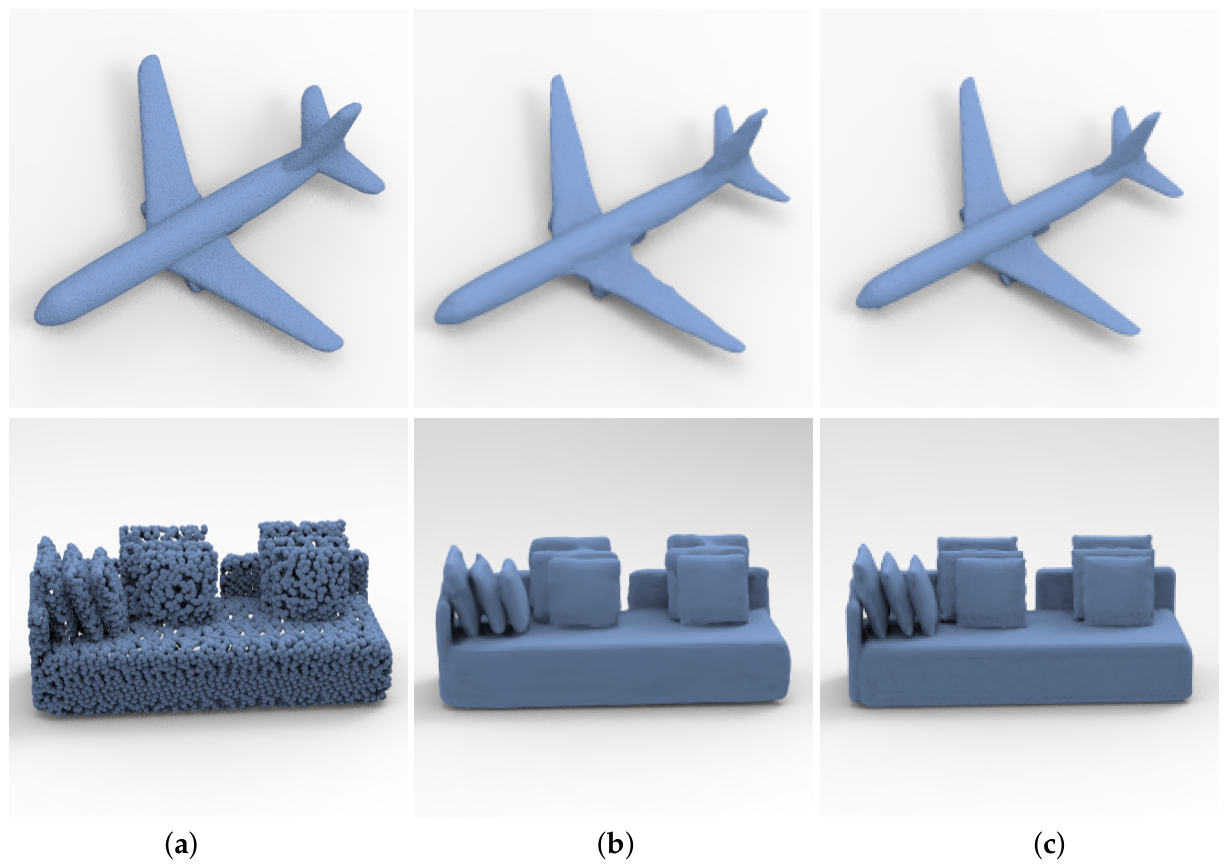
Figure 2.
Overall framework of our presented implicit surface reconstruction network.
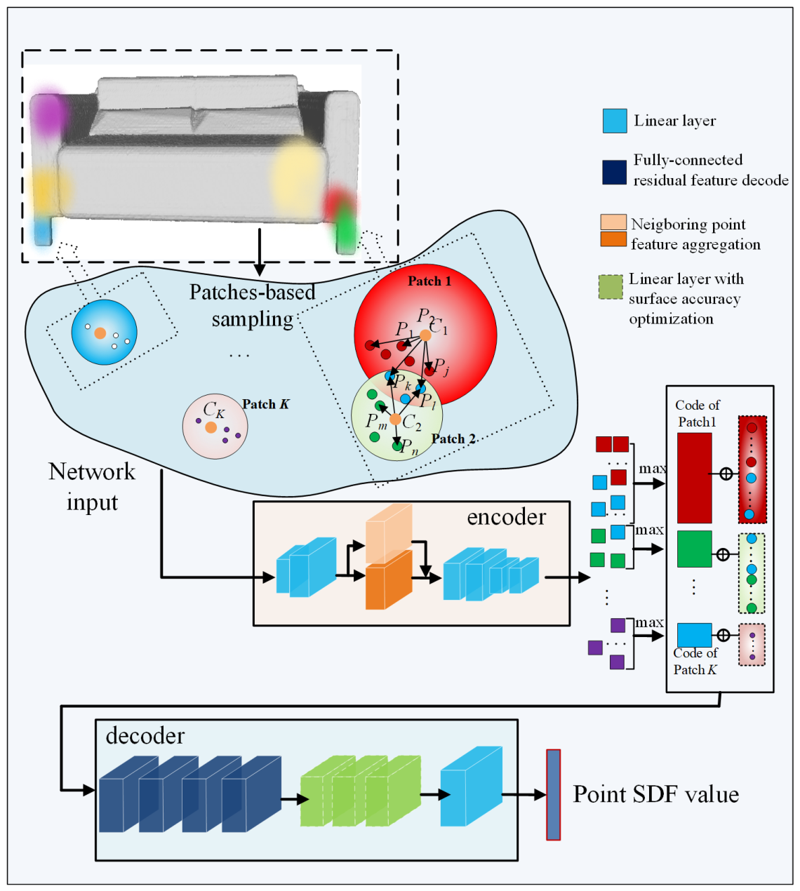
Figure 3.
SDF based Implicit surface reconstruction with surface accuracy .
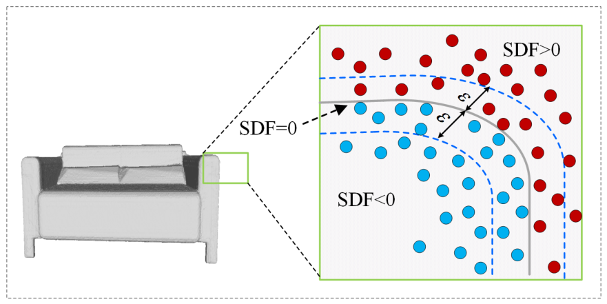
Figure 4.
Encoder of the proposed network.
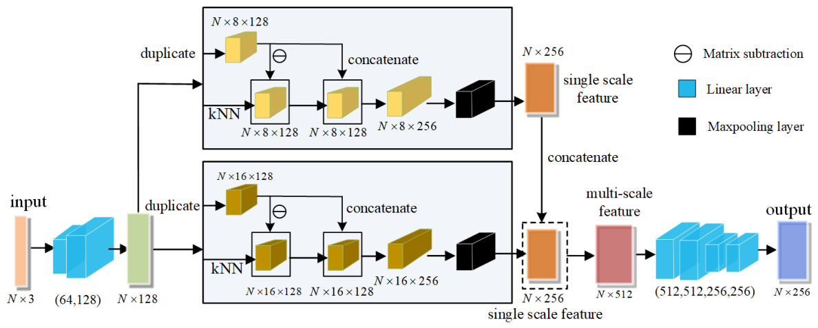
Figure 5.
Decoder of the proposed network.
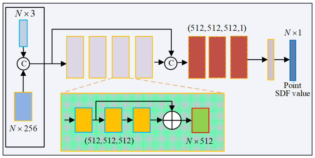
Figure 6.
Reconstruction results of our proposed method on ShapeNet dataset [1]. For each point cloud model, (a) gives the input point cloud model and (b) shows the reconstruction results via our network; (c) shows the ground truth.
Figure 6.
Reconstruction results of our proposed method on ShapeNet dataset [1]. For each point cloud model, (a) gives the input point cloud model and (b) shows the reconstruction results via our network; (c) shows the ground truth.
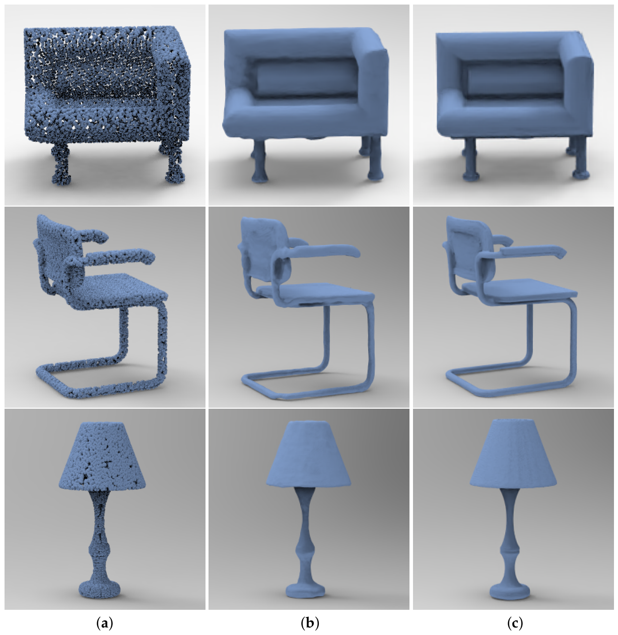
Figure 7.
Reconstruction results of our proposed method on Famous dataset [41]. For each point cloud model, (a) gives the input point cloud model and (b) shows the reconstruction results via our method; (c) shows the ground truth.
Figure 7.
Reconstruction results of our proposed method on Famous dataset [41]. For each point cloud model, (a) gives the input point cloud model and (b) shows the reconstruction results via our method; (c) shows the ground truth.
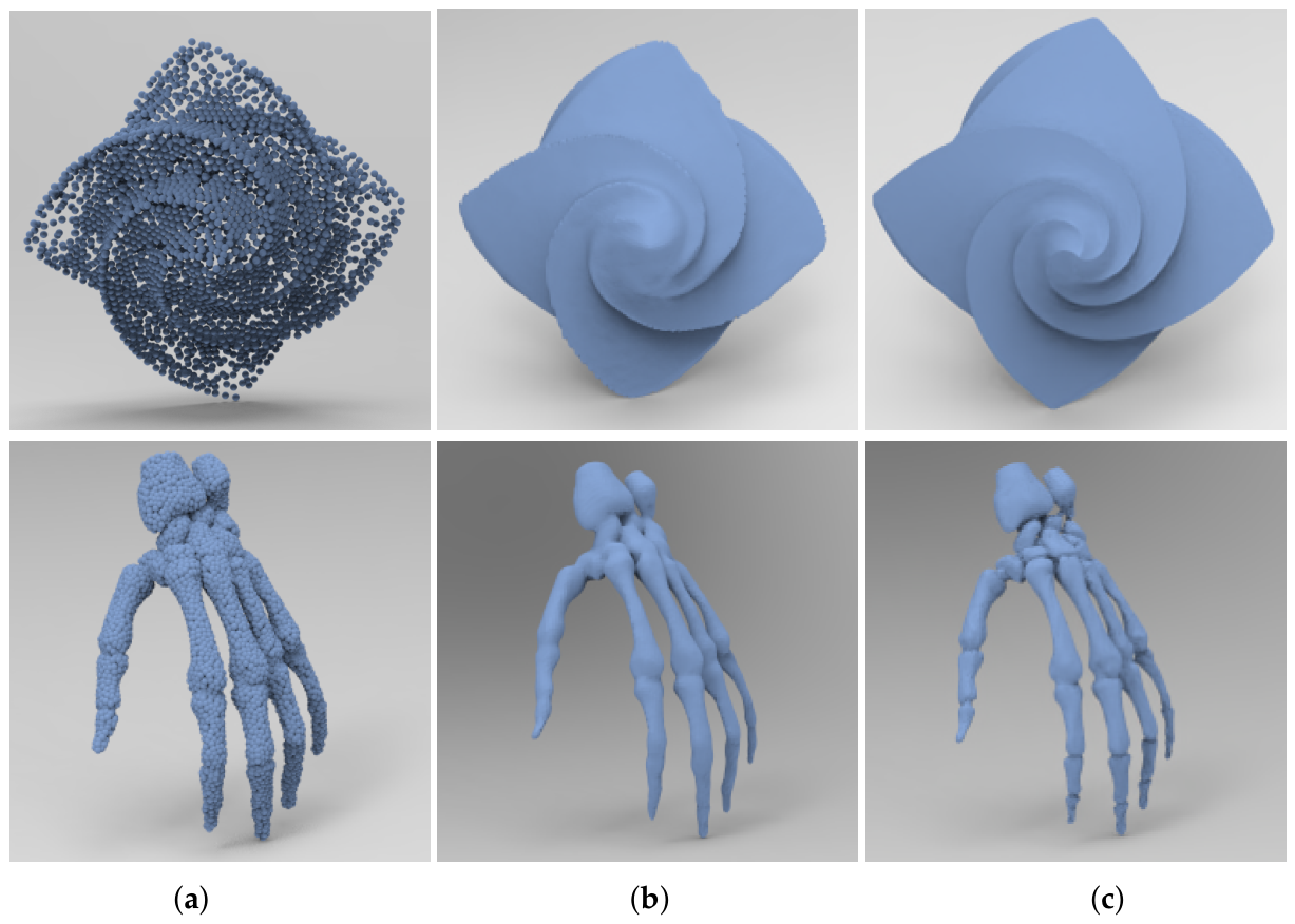
Figure 8.
Comparisons of reconstruction results via different methods on ShapeNet dataset [1]. For each point cloud model, (a) gives the input point cloud model, (b) shows the reconstruction results via DeepSDF [19]; (c) shows the reconstruction results via occupancy network [20]; (d) shows the reconstruction results via convolutional occupancy network [23]; (e) shows the reconstruction results via our proposed network, and (f) shows the ground truth.
Figure 8.
Comparisons of reconstruction results via different methods on ShapeNet dataset [1]. For each point cloud model, (a) gives the input point cloud model, (b) shows the reconstruction results via DeepSDF [19]; (c) shows the reconstruction results via occupancy network [20]; (d) shows the reconstruction results via convolutional occupancy network [23]; (e) shows the reconstruction results via our proposed network, and (f) shows the ground truth.
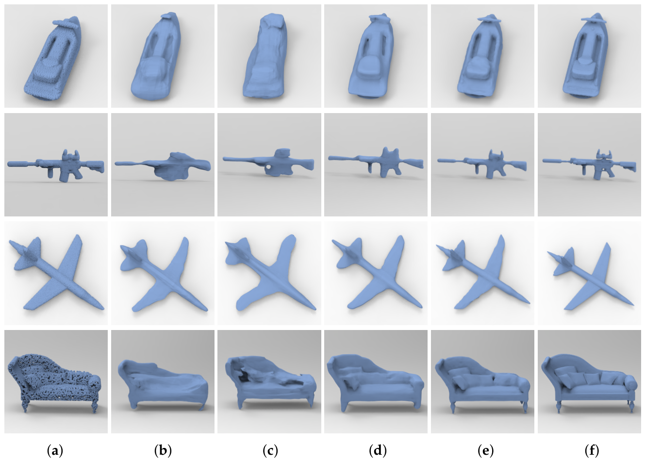

Table 1.
Correspondence between the number of decoder layers and training rounds.
| #epoch/round | 0∼100 | 100∼300 | 300∼500 | 500∼1000 |
|---|---|---|---|---|
| #decoder layers | 5 | 6 | 7 | 8 |
| Value | 0.0250 | 0.0100 | 0.0025 | 0.0000 |
Table 2.
Data statistics for different networks on ShapeNet dataset [1].
Table 2.
Data statistics for different networks on ShapeNet dataset [1].
| Index | Category | DeepSDF | ONet | CONet | Ours |
|---|---|---|---|---|---|
| airplane | 78.90 | 73.00 | 83.60 | 80.10 | |
| sofa | 90.30 | 87.90 | 92.50 | 90.60 | |
| IoU↑ | chair | 74.10 | 68.80 | 80.10 | 85.70 |
| lamp | 70.90 | 54.60 | 74.00 | 77.30 | |
| rifle | 76.80 | 68.40 | 81.00 | 85.20 | |
| vessel | 82.70 | 74.10 | 85.70 | 87.00 | |
| airplane | 0.015 | 0.025 | 0.005 | 0.005 | |
| sofa | 0.046 | 0.042 | 0.012 | 0.009 | |
| CD↓ | chair | 0.046 | 0.053 | 0.022 | 0.007 |
| lamp | 0.175 | 0.274 | 0.085 | 0.055 | |
| rifle | 0.012 | 0.021 | 0.005 | 0.002 | |
| vessel | 0.023 | 0.038 | 0.009 | 0.006 |
*Boldface indicates the best value, underline means the second best value.
Table 3.
Ablation study of the proposed surface reconstruction network.
| Methods | IoU↑ | CD Error↓ |
|---|---|---|
| baseline model | 68.70 | 0.084 |
| reconst. via 30 patches | 76.10 | 0.019 |
| 30 patches + SAO | 77.90 | 0.012 |
| our method | 85.70 | 0.007 |
Disclaimer/Publisher’s Note: The statements, opinions and data contained in all publications are solely those of the individual author(s) and contributor(s) and not of MDPI and/or the editor(s). MDPI and/or the editor(s) disclaim responsibility for any injury to people or property resulting from any ideas, methods, instructions or products referred to in the content. |
© 2026 by the authors. Licensee MDPI, Basel, Switzerland. This article is an open access article distributed under the terms and conditions of the Creative Commons Attribution (CC BY) license (http://creativecommons.org/licenses/by/4.0/).
Copyright: This open access article is published under a Creative Commons CC BY 4.0 license, which permit the free download, distribution, and reuse, provided that the author and preprint are cited in any reuse.


