

Submitted:
17 August 2026
Posted:
18 August 2026
You are already at the latest version
Abstract
Building on our previous Multiconfiguration-Dirac-Hartree-Fock (MCDHF) computational strategies taylored for the hyperfine structure (HFS) of low-lying levels in one-valence electron Sr II and Ba II ions, and in two-valence electrons Ba I atom [Nezosi et al, Atoms 14, 17 (2026). DOI: 10.3390/atoms14030017], we successfully extend these methodologies along the alkaline-earth elements to the lighter Ca II and the heavier Ra I-II ions. MCDHF recommended HFS constants, along with their uncertainty estimates, are reported for the first time and critically discussed. Where applicable, the Bohr-Weisskopf correction is applied to the HFS constants, and its effects are analyzed. This is particularly valuable for cases where no measurement is available such as for the [Rn]\(6d ^2D_{3/2,5/2}\) levels in 223,225Ra II, for the [Rn]\(7s6d~^3D_{1,2,3}\) and 1D2 levels in 223Ra I, for the [Rn]\(7s6d ^3D_{2,3}\) and 1D2 levels in 223Ra I, and for the [Rn]\(7s7p~^3P^o_2\) level in 225Ra I. In all cases, our MCDHF values agree with the ones found in the literature within our error bars. For the 2D5/2 levels in Ca II and Ra II, the discrepancies with experiment observed in Sr II and Ba II for the HFS \(A\) constant are not seen.
Keywords:
atomic structure
; hyperfine structure
; MCDHF method
; GRASP package
; calcium
; radium
1. Introduction
Alkaline-earth metals from Mg to Ra, particularly in their singly ionized forms (e.g., Ca II, Ra II), are ideal for high-precision calculations and measurements in astrophysics and metrology due to their simple electronic structure [1]. Neutral radium (Ra I) is also crucial for beyond-Standard-Model (BSM) physics.
In astrophysics, Ca II infrared triplet lines (8498, 8542, 8665 Å) serve as key calcium abundance indicators in stellar atmospheres, detectable even at extremely low metallicities [2], enabling studies of metal-poor stars [3] and galactic chemical evolution [4]. Ra II UV-Vis lines (3814, 4682, 6705 Å) probe r-process nucleosynthesis, as Ra is produced exclusively by neutron capture in neutron-rich environments where the s-process ends at bismuth (Z=83) [5,6]. Its likely production in neutron star mergers makes Ra detection in kilonovae spectra a direct indicator of such events [7].
In fundamental physics, Ca II and Ra II are crucial for frequency standards and precision measurements. Quadrupole moments in metastable atomic ions introduce systematic energy shifts in such systems [8]. High theoretical precision is required for meaningful comparisons with parity non-conservation (PNC) experiments [9]. While heavier atoms like Ra offer more favorable PNC conditions, lighter elements such as Ca II serve as essential test cases for validating theoretical methods before tackling heavier systems.
Neutral radium (Ra I) offers unique opportunities for fundamental physics tests. The search for a permanent electron electric dipole moment (EDM) is among the most stringent BSM tests, with polar molecules like RaF serving as exceptionally sensitive probes due to their large internal electric fields and Ra’s heavy, octupole-deformed nucleus [10]. Precise ab initio calculations for Ra are essential, providing wavefunctions needed to interpret molecular EDM measurements and constrain -violating interactions. Multiconfiguration Dirac-Hartree-Fock (MCDHF) calculations for Ra I address this by capturing critical enhancement mechanisms, notably the [Rn]7s7p 3 and [Rn] levels, separated by only . Combined with Ra high atomic number and nuclear octupole deformation, this yields P- and T-reversal-odd effect enhancements up to five orders of magnitude greater than in other systems [11,12]. Electron correlation effects, which dominate the atomic EDM signal, are systematically accounted for in combination of MCDHF and relativistic configuration interaction (MCDHF+RCI) calculations. Ra II, with its 8230 Å clock transition and narrow linewidth, is also a candidate for optical atomic clocks. The low-cost diode lasers required for Ra II, compared to expensive UV lasers, make it attractive for both laboratory and transportable applications [13].
Accounting for the hyperfine structure (HFS) of the levels is essential. In astrophysics and atomic clock applications, HFS broadening and the resulting asymmetries in line profiles introduce inaccuracies in line positions and strengths. For BSM research, HFS constants enable extraction of electric field gradients to calibrate molecular theory against high-resolution RaF spectroscopy at ISOLDE (CERN), where 14 excited states have been characterized with theory-experiment agreement and laser-coolable transitions identified [10]. Accurate ab initio atomic wavefunctions and correlation energies could enhance RaF sensitivity to e-EDM searches, where experimental data are scarce.
For Ca II and Ra I-II, the HFS of certain levels remain experimentally unstudied, including the [Rn] levels in 223,225Ra II and the [Rn] and [Rn] levels in Ra I. While extensive MCDHF calculations are available for Mg II [14], Ca II [8], Sr II, and Ba II [15], comprehensive calculations for Ra II remain limited.
In this work, we present theoretical calculations of magnetic dipole (A) and electric quadrupole (B) hyperfine structure constants for low-lying levels of Ca II and Ra I-II. Using the MCDHF method with Relativistic Configuration Interaction (RCI) within the GRASP framework [16], we extend our previously validated computational strategies from Sr II and Ba I-II [15] to the lighter Ca II and the heavier Ra I-II systems, employing for the first time a natural orbital basis transformation [17] approach for HFS calculations in heavy Ra I-II. Particular attention is given to the Bohr-Weisskopf (BW) effect, which is systematically accounted for in our calculations. By providing theoretical values for levels where experimental data are unavailable, and demonstrating agreement with existing measurements within our uncertainty estimates, we enable refined tests of atomic structure and nuclear effects. These results offer essential theoretical input for astrophysical abundance studies via Ca II infrared triplet lines, precision metrology using Ra II clock transitions, and searches for physics beyond the Standard Model through Ra I molecular and atomic electric dipole moment investigations.
This paper is organized as follows. Section 2 describes the MCDHF and RCI methods for calculating HFS constants and provides details about the transformation to natural orbitals. Section 3 presents Ca II calculations to validate the theoretical method from the earlier Sr II/Ba II study [15], followed by Ra II and Ra I HFS studies. Section 4 concludes with an outlook.
2. Method and Computational Details
2.1. Multiconfiguration Dirac–Hartree–Fock Method
The Multiconfiguration Dirac-Hartree-Fock (MCDHF) method, described in [18], is a fully relativistic approach to atomic structure calculations. It is particularly well suited for the study of medium- and high-Z elements as well as highly charged ions. Within this framework, an atomic state characterized by the quantum numbers , J, , and parity is represented by an Atomic State Function (ASF), denoted by . The ASF is expressed as a linear combination of Configuration State Functions (CSFs) ,
where the label specifies the electronic configuration, the angular momentum coupling scheme, and any additional quantum numbers required to uniquely identify the CSF. The expansion coefficients , together with the corresponding atomic-state energy E, are obtained by solving the secular equation
where denotes the Hamiltonian matrix.
Applying the variational principle to the total energy functional leads to the MCDHF equations, a set of coupled integro-differential equations that are solved self-consistently for the radial components of the one-electron spin-orbitals.
Subsequent Relativistic Configuration Interaction (RCI) calculations are performed by solving Eq. (2) using an enlarged CSF expansion, if desired, while keeping the orbitals obtained from the preceding MCDHF optimization fixed. At this stage, additional relativistic contributions may be incorporated into the Hamiltonian, including the Breit interaction and quantum electrodynamic (QED) corrections, thereby improving the accuracy of the calculated atomic properties.
2.2. Natural Orbitals
Due to numerical convergence challenges, and to reduce computation time, the MCDHF method employs a layer-by-layer (LBL) [19] approach in which only the newly introduced orbitals for the layer considered are optimized while the remaining are kept frozen. Therefore, the frozen orbitals, especially the spectroscopic reference orbitals, cannot react to the addition of the newly introduced layer. Natural orbitals (NO) provide an alternative orbital basis, first introduced in quantum chemistry, that addresses this limitation. They modify the orbitals of the reference states in a way that partly captures the response to the new layers. The NOs are obtained by diagonalizing the density matrix, which provides a more natural description of the electron correlation. One of the first applications to atomic physics was by Lindgren et al. [20] in order to determine hyperfine interaction in alkali atoms in many-body perturbation calculations. Schiffmann et al. [17] developed the NO formalism in the MCDHF framework and applied it in the hyperfine structure calculation of Na I [21], exhibiting results in better agreement with experiment than using the traditional LBL approach. Transformation to NOs also showed to considerably improve the hyperfine interaction constants and transition rates in other systems, e.g., In I [22].
For each value of , the relativistic angular quantum number, the density matrix is built such as
with
where are the spin-angular coefficients. The NOs are obtained from the eigenvectors of the density matrix diagonalizing it
where the eigenvalues are the occupation numbers of the NOs
with the number of electrons. The large and the small components of the radial function of the NOs are therefore
with the coefficients the matrix elements of the unitary matrix in eq. (5) and , the large and the small components of the radial function in the MCDHF equations [18].
2.3. Hyperfine Structure
The hyperfine structure (HFS) of an atomic fine-structure level arises from the interaction between the atomic electrons and the electromagnetic multipole moments of the nucleus. This interaction can be described through the multipole expansion
where and are spherical tensor operators of rank k acting in the electronic and nuclear spaces, respectively. The terms corresponding to and represent the magnetic dipole (M1) and electric quadrupole (E2) interactions.
For an atom containing electrons, the electronic tensor operators are expressed as
where , is the fine-structure constant, and denotes the vector of Dirac matrices related to the Pauli matrices.
The nuclear magnetic dipole moment and electric quadrupole moment Q are defined through the matrix elements of the nuclear tensor operators,
where denotes the nuclear state with maximal spin projection, [23]. The operators and correspond to the magnetic dipole and electric quadrupole moments of the nucleus, respectively.
Since the hyperfine interaction is generally much weaker than the fine-structure splitting, it can be treated within first-order perturbation theory. The corresponding hyperfine energy shift is given by
where is the zeroth-order wave function of the coupled electron-nucleus system [19], with F and denoting the total hyperfine angular momentum and its projection on the quantization axis, respectively.
It is convenient to express the hyperfine energy shifts in terms of the magnetic dipole (A) and electric quadrupole (B) hyperfine constants:
where
and
The reduced matrix elements , with or , are evaluated using the atomic state functions (ASFs) defined in Eq. (1).
2.4. Computational Details
The MCDHF calculations and the evaluation of the hyperfine structure (HFS) constants were performed using GRASP2018 [24,25]. To improve computational efficiency, the recently developed GRASPG package by Si et al. [26], which exploits Configuration State Function Generators (CSFGs), was employed for the RCI calculations.
Following the methodology introduced by Papoulia et al. [27], the final HFS constants are reported as recommended values derived from the largest RCI calculations obtained with different orbital optimization strategies. The results from these calculations are treated as independent estimates, allowing the determination of both a mean value and a standard deviation for each constant. This procedure provides a robust prediction of the HFS constants together with a quantitative uncertainty assessment, which is particularly valuable in the absence of experimental data. The recommended values are expressed as , corresponding to a confidence interval.
3. Results and Discussion
3.1. Ca II
Calcium (Ca) has 26 known isotopes, of which 5 are stable [28]. 43Ca has an abundance of only 0.135% but is the only stable isotope that has a hyperfine structure due to its non-zero nuclear spin . The levels of interest in 43Ca II are the even [Ar] and [Ar] as well as the odd [Ar].
Due to its relatively simple electronic structure, 43Ca II has already been studied in depth theoretically by Silverans et al. [29] and Yu et al. [30] using the Relativistic Many-Body Perturbation Theory (RMBPT) approach, Itano [8] with the MCDHF method, Chakraborty et al. [31] with the Relativistic Coupled Cluster (RCC) method, and Safronova et al. [32] using the relavistic all-order method where all Single, Double and partial Triple (SDpT) excitations of the wavefunctions are included to all order of perturbation theory. Goble et al. [9] and Nortershauser et al. [1] performed optical spectroscopy experiments using hollow cathode discharge and fast ion beam collinear laser spectroscopy, whereas Garcia Ruiz et al. [33] adopted bunched-beam collinear laser spectroscopy.
The MCDHF method used in this paper relies on the AS [19] and LBL [25] approaches, which enable the optimization of only a subset of orbitals at each calculation step. For example, for the ground 2 level, an initial Dirac-Hartree-Fock (DHF) layer is considered. This layer is built using the spectroscopic orbitals in nonrelativistic notation, where the highest n quantum number is quoted for each l-symmetry, and no electron correlation is included at this stage. The ASs are then expanded with correlation orbitals up to (g-orbitals) to directly apply the Ba/Sr model [15] and achieve high precision in the calculations [34]. For each AS given in Table 1, only the newly introduced orbitals are optimized, while the remaining orbitals are kept frozen. The mixing coefficients of the ASFs are then determined, and Quantum Electrodynamics (QED) corrections are included at the RCI step. Finally, the HFS constants are computed.
Following Bieroń et al. [35], the impact of different classes of orbital substitutions has been investigated. Using an DHF orbital basis, more correlations are accumulated by allowing single and double (SD) substitutions from deeper orbitals employing Single References (SR) for each level using the fourth correlation layer (AS4) given in Table 1.
In Table 2, the individual contribution of single (S) orbital substitution to the magnetic dipole HFS constant of the ground level, , is presented. Figure 1 gives a more visual representation of these contributions.
While the contribution of the orbital is negligible, +0.08 MHz, the s orbital substitutions dominate, with the orbital contributing MHz. This highlights the critical role of s single substitutions in the HFS. To align with the Ba/Sr methodology [15], the and orbitals are included in the optimization step, even though the substitution contributes less than a percent. Consequently, correlations are excluded from the optimization.
As shown in Table 3 and Figure 2, the contributions for the excited states are similar, with the contribution being negligible compared to the and ones. The contributions for the B hyperfine constants indicate that the most important contribution comes from correlations, which is mainly due to the orbital polarization or Sternheimer effect [23]. The trends above are also observed in the 2 and the odd P levels.
Thanks to this analysis, the optimization of the radial orbitals can be aimed for relevant correlations for the hyperfine structure. The GRASP package [24] is considering spectroscopic orbitals in two ways. Let us take the example of the ground (or [Ar]4s 2) level. The core orbitals are , while the valence orbital is . We can therefore build our MCDHF optimizations on core-valence (CV) correlations. To directly apply the MCDHF+RCI model developed for 87Sr II and 137Ba II [15], we used the equivalent CV single and restricted double (SrD) orbital optimization strategy with substitutions. Here, "restricted" means at most one hole per active core orbital, i.e., allowing substitutions from and to with at most one substitution from each core orbital to the valence one [36]. A second optimization strategy (MCDHF CV SrD ) taking care of the and core orbitals that are important to correctly describe the HFS for the excited levels was also considered. With the ASs described in Table 1, seven layers of correlation orbitals were considered in order to achieve a convergence in our results. The latter is obtained when the HFS constants do not vary within some a priori accepted variation interval. Results for the HFS constants at each optimization step are given in Table 5.
As expected, CV correlations are crucial to describe the hyperfine interaction. The MCDHF CV SrD shows a stable value achieved for the fourth active set (AS4). The ground level already agrees with experiment to within MHz (0.5%). This agreement is observed for each HFS constant except the value with a persistent MHz difference (223%). This behavior is well known from the Sr/Ba study [15]. To try to overcome this discrepancy, the second orbital set, MCDHF CV SrD is considered. The agreement worsens for all HFS constants but is improved for the constant that still shows a MHz difference.
Following MCDHF calculations, deeper core-core (CC) correlations are added in the RCI step. The first RCI CC SD model allows SD substitutions from and orbitals to the valence orbital, with no substitutions between the core orbitals in order to save computational time by decreasing the number of CSFs by a factor of two. As we want to account for as much correlation as possible, a second RCI strategy based on CC SD substitutions is considered. Adding correlations from the core orbital was shown to be negligible, with less than a percent change in the values for the ground level. Therefore, they were also omitted. Using the MCDHF CV SrD nl optimization, the extended RCI CC SD model modifies the electric quadrupole A hyperfine constants by for the ground level. The largest change appears for which varies by . For the magnetic dipole B constant, we observe shifts of MHz for the D levels, while remains unchanged. The second MCDHF CV SrD optimization yielded identical results with the same RCI approach.
The uncertainty in the theoretical HFS values can be evaluated through multiple approaches. One method involves treating the largest RCI calculations from distinct MCDHF optimizations as independent values. A mean value and standard deviation are then calculated from this set. The final result is expressed as , which corresponds to a 95% confidence interval.
However, this uncertainty estimation could only be applied to the layer-by-layer (LBL) calculation. The presented MCDHF+RCI methods were originally developed for barium (Ba) [15], which has a larger electronic core including d orbitals. When directly applied to lighter elements (such as calcium, with lower atomic number Z), the largest MCDHF+RCI method encountered limitations. Specifically, for calculations using the Natural Orbital (NO) basis, single (S) substitutions from all orbitals were included. In this case, both RCI calculations produced identical results. As a consequence, no uncertainty estimate could be obtained. This highlights a limitation of the model when applied to lighter elements.
Recent studies by Sahoo et al. [14] and Atalay [22] suggested a different approach for the use of a NO basis for HFS calculations. Compared to Nezosi et al. [15], where the biggest optimized MCDHF orbitals resulting from traditional single and restricted double (SrD) substitutions are transformed to NO using the rdensity program [17], here the NO basis is obtained via S substitutions (with at most one substitution from all core orbitals) from a multireference (MR) for the S, D and P levels studied in this paper. The largest MCDHF optimization calculation following this approach is then transformed to natural orbitals and then used in RCI calculations. This new approach is appealing as it can relax all orbitals in a single, compact calculation, as only a total of CSFs was needed compared to the CSFs for the MCDHF CV optimization only for the 2 HFS calculations at AS7. This approach is especially suitable for high-Z, as the number of CSFs grows rapidly with the number of active orbitals.
At first glance, equations (17,18) show that and . Johnson [37] showed, in the Pauli approximation where the small and the large can be linked by
that is linked to , indicating that the A and B HFS constants are both in the Pauli approximation.
Any modification in caused by the transformation to NO could result in a modification in . Table 4 compares the change in these expectation values for each d-subshell for a layer-by-layer (LBL) calculation and after transformation to NO. The spectroscopic orbital is highlighted. Even the smallest change in induces variation in as it can be seen for the valence orbital
inducing a direct change in and
The orbital contraction is more visible on Figure 3 between 3 and . The top left graph shows the large component of the valence orbital as a function of r, for the LBL calculation (in blue) and the transformed NO (in dashed red) obtained from the S substitutions MR calculation. The bottom-left graph shows the absolute difference between these two orbital bases. There are multiple zones where the NO valence orbital is more contracted than the LBL one. On the right-hand side, the region is zoomed in where the contraction appears clearly with the red arrow. Even this small contraction (about in this region) can cause a difference in the A HFS constants. The same behavior applies to the valence orbitals of ground and the P excited levels, as well as in the B HFS constants.
Using the NO basis, we repeated all RCI calculations (labeled NO in Table 5). Results for both optimizations differ by only a few MHz. We recommend the final NO values as it accounts for orbital contraction and shows better agreement with experimental values, except for .
For an accurate theoretical determination of the HFS constants, one should account for the Bohr-Weisskopf (BW) effect [38], a correction of the finite nuclear magnetization distribution of the nucleus, giving a contribution to the HFS. Chakraborty et al. [31] studied the BW correction effect on the calculated HFS constants in 43Ca II, with limited correction (at most 0.30% for the 2 level). The BW corrected A HFS constants for the 2 and 2 levels are given in Table 6 but could not correct the fact that the values calculated with the LBL orbital basis are closer to the experiment than the ones calculated with the NO orbitals.

Table 5.
Magnetic dipole A and electric quadrupole B hyperfine structure constants (in MHz) of 43 [39], compared to avaialble theoretical and experimental data. The recommended values are given in the form , exhibiting a confidence level. ★: Number of CSFs obtained after reduction using the rcsfginteract_csfg code. a: Th. Silverans et al. (RMBPT) [29]; b: Th. Yu et al. (RMBPT) [30]; c: Th. Itano (MCDHF) [8]; d: Th. Chakraborty et al. (RCC) [31]; e: Th. Safronova et al. (SDpT) [32]; f: Expt. Goble et al. [9]; g: Expt. Nortershauser et al. [1]; h: Expt. Garcia Ruiz et al. [33]; i: Expt. Silverans et al. [29]
Table 5.
Magnetic dipole A and electric quadrupole B hyperfine structure constants (in MHz) of 43 [39], compared to avaialble theoretical and experimental data. The recommended values are given in the form , exhibiting a confidence level. ★: Number of CSFs obtained after reduction using the rcsfginteract_csfg code. a: Th. Silverans et al. (RMBPT) [29]; b: Th. Yu et al. (RMBPT) [30]; c: Th. Itano (MCDHF) [8]; d: Th. Chakraborty et al. (RCC) [31]; e: Th. Safronova et al. (SDpT) [32]; f: Expt. Goble et al. [9]; g: Expt. Nortershauser et al. [1]; h: Expt. Garcia Ruiz et al. [33]; i: Expt. Silverans et al. [29]
| Step | 2 | 2 | 2 | 2 | 2 | ||||||||
|---|---|---|---|---|---|---|---|---|---|---|---|---|---|
| DHF | 1 | −606.08 | 1 | −34.31 | −2.67 | 1 | −14.61 | −3.77 | 1 | −108.90 | 1 | −21.11 | −4.93 |
| MCDHF (+AS1) | 37 | −740.61 | 120 | −45.94 | −1.92 | 130 | −11.57 | −2.74 | 53 | −133.06 | 74 | −25.64 | −6.75 |
| MCDHF (+AS2) | 152 | −774.30 | 433 | −48.78 | −2.67 | 496 | −12.32 | −3.79 | 181 | −142.25 | 278 | −32.92 | −7.19 |
| MCDHF (+AS3) | 380 | −802.39 | 944 | −50.54 | −2.65 | 1,100 | −12.12 | −3.77 | 423 | −145.46 | 688 | −34.14 | −7.29 |
| MCDHF (+AS4) | 722 | −796.91 | 1,653 | −50.63 | −2.78 | 1,942 | −12.52 | −3.94 | 781 | −146.26 | 1,300 | −33.58 | −7.33 |
| MCDHF (+AS5) | 1,178 | −800.83 | 2,560 | −50.81 | −2.72 | 3,022 | −12.20 | −3.87 | 1,255 | −147.96 | 2,114 | −33.77 | −7.36 |
| MCDHF (+AS6) | 1,748 | −800.26 | 3,665 | −50.93 | −2.76 | 4,340 | −12.33 | −3.92 | 1,845 | −147.82 | 3,130 | −33.76 | −7.35 |
| MCDHF (+AS7) | 2,432 | −801.87 | 4,968 | −50.91 | −2.75 | 5,896 | −12.26 | −3.90 | 2,551 | −146.87 | 4,348 | −33.79 | −7.35 |
| RCI CC SD (+AS7) | 9,407★ | −737.72 | 27,462★ | −44.88 | −2.75 | 38,541★ | −9.50 | −3.91 | 9,825★ | −125.47 | 23,013★ | −28.59 | −6.33 |
| RCI CC SD (+AS7) | 18,806★ | −763.60 | 54,916★ | −44.63 | −4.64 | 77,074★ | −4.94 | −4.00 | 19,642★ | −131.02 | 46,018★ | −30.50 | −6.68 |
| RCI CC SD (+AS7, NO) | 9,407★ | −764.91 | 27,462★ | −46.83 | −2.85 | 38,541★ | −10.47 | −4.06 | 9,825★ | −126.58 | 23,013★ | −28.81 | −6.35 |
| RCI CC SD (+AS7, NO) | 18,806★ | −810.51 | 54,916★ | −48.34 | −3.48 | 77,074★ | −5.23 | −4.95 | 19,642★ | −133.17 | 46,018★ | −31.30 | −6.76 |
| DHF | 1 | −606.08 | 1 | −34.31 | −2.67 | 1 | −14.61 | −3.77 | 1 | −108.90 | 1 | −21.11 | −4.93 |
| MCDHF (+AS1) | 72 | −745.89 | 238 | −46.16 | −2.05 | 258 | −9.52 | −2.90 | 104 | −135.35 | 146 | −25.82 | −6.89 |
| MCDHF (+AS2) | 301 | −782.91 | 863 | −49.68 | −3.11 | 989 | −8.55 | −4.42 | 359 | −145.30 | 553 | −33.02 | −7.37 |
| MCDHF (+AS3) | 756 | −841.46 | 1,884 | −52.18 | −3.19 | 2,196 | −7.10 | −4.54 | 842 | −155.70 | 1,372 | −35.74 | −7.89 |
| MCDHF (+AS4) | 1,439 | −845.50 | 3,301 | −53.03 | −3.47 | 3,879 | −7.34 | −4.94 | 1,557 | −157.58 | 2,595 | −36.59 | −8.00 |
| MCDHF (+AS5) | 2,350 | −854.23 | 5,114 | −53.21 | −3.36 | 6,038 | −7.08 | −4.79 | 2,504 | −158.81 | 4,222 | −37.50 | −8.02 |
| MCDHF (+AS6) | 3,489 | −854.63 | 7,323 | −53.33 | −3.41 | 8,673 | −7.26 | −4.86 | 3,682 | −159.24 | 6,253 | −37.52 | −8.00 |
| MCDHF (+AS7) | 4,856 | −854.43 | 9,928 | −53.33 | −3.39 | 11,784 | −7.18 | −4.81 | 5,094 | −159.55 | 8,688 | −37.51 | −8.02 |
| RCI CC SD (+AS7) | 11,831★ | −782.79 | 32,422★ | −46.82 | −3.29 | 44,429★ | −5.30 | −4.70 | 12,368★ | −135.67 | 27,353★ | −31.58 | −6.87 |
| RCI CC SD (+AS7) | 18,806★ | −760.96 | 54,916★ | −44.42 | −3.25 | 77,074★ | −-4.61 | −3.98 | 19,642★ | −130.84 | 46,018★ | −30.35 | −6.61 |
| RCI CC SD (+AS7, NO) | 11,831★ | −815.92 | 32,422★ | −49.24 | −3.42 | 44,429★ | −5.29 | −4.88 | 12,368★ | −136.23 | 27,353★ | −32.12 | −6.64 |
| RCI CC SD (+AS7, NO) | 18,806★ | −810.50 | 54,916★ | −48.34 | −3.48 | 77,074★ | −5.23 | −4.95 | 19,642★ | −133.17 | 46,018★ | −31.30 | −6.76 |
| This work (LBL) | −763.16 ± 2.85 | −44.51 ± 0.32 | −2.81 ± 0.02 | −4.91 ± 0.12 | −3.99 ± 0.03 | −130.93 ± 0.25 | −30.43 ± 0.21 | −5.73 ± 0.10 | |||||
| This work (NO), recommended | −811.38 | −48.32 | −3.00 | −5.24 | −4.27 | −133.17 | −31.30 | −5.83 | |||||
| Th.a | −819 | −148 | −30.9 | -6.7 | |||||||||
| Th.b | −805.35 | −47.82 | −3.0 | −3.55 | −4.4 | −143.07 | −30.49 | −6.7 | |||||
| Th.c | −47.27 | −2.94 | −4.84 | −4.18 | |||||||||
| Th.d | −806 ± 3 | −47.8 ± 0.3 | −3.06 ± 0.07 | −3.30 ± 0.04 | −4.24 ± 0.09 | ||||||||
| Th.e | −801.28 | −47.63 | −2.87 | −4.24 | −4.08 | −144.96 | −30.34 | −6.64 | |||||
| Expt.f | −797.5 ± 2.4 | −158.0 ± 3.3 | −29.7 ± 1.6 | ||||||||||
| Expt.g | −47.3 ± 0.2 | −3.7 ± 1.9 | −3.8 ± 0.6 | −3.9 ± 6.0 | −145.4 ± 0.1 | −31.0 ± 0.2 | −6.9 ± 1.7 | ||||||
| Expt.h | −806.87 ± 0.42 | −31.10 ± 0.30 | −4.2 ± 1.3 | ||||||||||
| Expt.i | −805 ± 2 | −145.5 ± 1.0 | −31.9 ± 0.2 | −6.7 ± 1.4 | |||||||||
Table 6.
Bohr-Weisskopf (BW) corrected magnetic dipole A hyperfine structure constants (in MHz) of 43 [40], [39]), using the extracted relative BW corrections of Chakraborty et al. [31], compared to available theoretical and experimental data. The recommended values are given in the form of , exhibiting a confidence level. a: Th. Silverans et al. (RMBPT) [29]; b: Th. Yu et al. (RMBPT) [30]; c: Th. Itano (MCDHF) [8]; d: Th. Chakraborty et al. (RCC) [31]; e: Th. Safronova et al. (SDpT) [32]; f: Expt. Goble et al. [9]; g: Expt. Nortershauser et al. [1]; h: Expt. Garcia Ruiz et al. [33]; i: Expt. Silverans et al. [29]
Table 6.
Bohr-Weisskopf (BW) corrected magnetic dipole A hyperfine structure constants (in MHz) of 43 [40], [39]), using the extracted relative BW corrections of Chakraborty et al. [31], compared to available theoretical and experimental data. The recommended values are given in the form of , exhibiting a confidence level. a: Th. Silverans et al. (RMBPT) [29]; b: Th. Yu et al. (RMBPT) [30]; c: Th. Itano (MCDHF) [8]; d: Th. Chakraborty et al. (RCC) [31]; e: Th. Safronova et al. (SDpT) [32]; f: Expt. Goble et al. [9]; g: Expt. Nortershauser et al. [1]; h: Expt. Garcia Ruiz et al. [33]; i: Expt. Silverans et al. [29]
| Reference | 2 | 2 | 2 |
|---|---|---|---|
| 43Ca II | |||
| This work (LBL) | −762.29 ± 3.73 | −44.51 ± 0.34 | −4.89 ± 0.11 |
| This work (NO) | −810.49 | −48.30 | −5.22 |
| Th.a | −819 | ||
| Th.b | −805.35 | −47.82 | −3.55 |
| Th.c | −47.27 | −4.84 | |
| Th.d | −806 3 | −47.8 ± 0.3 | −3.30 ± 0.04 |
| Th.e | −801.28 | −47.63 | −4.24 |
| Expt.f | −795.5 ± 2.4 | ||
| Expt.g | −47.3 ± 0.2 | −3.8 ± 0.6 | |
| Expt.h | −806.87 ± 0.42 | ||
| Expt.i | −805 ± 2 | ||
3.2. Ra II
Radium (Ra) is the heaviest alkaline earth metal, with 34 known radioactive isotopes. The most stable, 226Ra, has a half-life of 1,600 years [28]. The isotopes 223Ra and 225Ra, with nuclear spin and half-lives of and days respectively, only exist in trace amounts. Their short half-lives make experiments challenging, so theoretical hyperfine structure calculations are needed to provide experimental bounds. The levels of interest are the even [Rn]7s 2 and [Rn]6d 2 levels, as well as the odd [Rn]7p 2 levels, for which only a few experimental values are available. Using collinear fast-beam laser spectroscopy, Wendt et al. [41] determined the HFS of both levels, while Neu et al. [42] studied both the ground 2 and 2 levels. Theoretical values were obtained using RCC [43][44], Atomic Many-body Perturbation Theory in the Screened Coulomb Interaction (AMPSCI) [45] or the relativistic all-order SDpT method [46]. This is the first paper to compute HFS constants using the MCDHF and RCI method and to benchmark the new GRASPG [26] package for high-Z ions.
With the AS given in Table 7, the code limited the investigation of orbital substitutions to those no higher than . Table 8 and Figure 4 show that, for the ground level, the highest contribution comes from substitutions. and substitutions can be added to the optimization model in order to follow the Ba/Sr [15] strategies.
The obtained values for 223Ra II for both optimization strategies are given in Table 10. The first MCDHF CV SrD gives electric quadrupole A HFS constants that are near the literature values with at most difference for . However, the magnetic dipole B constants need more correlations to be accurately determined, as shown by the discrepancies for the D levels . However, when an experimental value exists, the calculated value agrees with only difference for the constant. Adding deeper correlations with the second MCDHF CV SrD deteriorates the agreements with the experimental values [41,42] and the other theoretical values [43,44,45] for all the A HFS constants except . The B HFS constants are closer to the calculated theoretical values of Sahoo et al. [43] (RCC). The agreement is preserved for the constant but is now too large compared to the experiment value. We are still convinced that adding correlation orbitals with higher l encapsulates the orbital polarization that was neglected in the first MCDHF CV SrD strategy and is important for a reliable determination of the B hyperfine constant [23].
After the MCDHF calculations, higher-order core-core (CC) correlations are added using RCI. Like in the Ca II case, two models are considered for each optimization strategy by allowing single and double (SD) substitutions. For all A HFS constants and for each orbital basis, both RCI models (RCI CC SD and RCI CC SD ) lower the positive values and increase the negative values. However, the added CC correlations are not enough to have a significantly better agreement for the B HFS constants for the D levels while using the MCDHF CV SrD orbital basis. The agreement even worsened for the 2 level with nearly a 100 MHz difference with the experimental value. Overall, the best agreement is obtained with the MCDHF CV SrD + RCI CC SD strategy. The agreement between the calculated value and RCC value [43] is still satisfactory for the constant.
We recall that, for Sr (Z = 38) and Ba (Z = 56), the HFS constant was problematic, with an opposite sign between calculated and literature values [15]. For Ra (Z = 88), the HFS constant does not show the same behavior. To understand this more clearly, we again move to the non-relativistic formalism, where the magnetic dipole HFS constant A is given as a sum of orbital, spin-dipole, and Fermi contact terms [47]. Table 9 shows the contribution of the different nonrelativistic hyperfine factors on the total A constant. For the Hartree-Fock (HF) calculation, the contact term is zero. Adding core-valence (CV) correlations by opening and for substitutions to one layer of correlation orbitals , we see a positive interference for the 2 level and a negative one for the 2 level. Compared with Sr and Ba the negative interference between the different terms is less pronounced for Ra making it less sensitive to neglected higher-order correlation effects from triple (T) and quadruple (Q) substitutions that are the likely causes for the lack of agreement with the experiment for the former elements.
In Ca II, the recommended values for this work were obtained using an NO basis. Following the same approach for Ra II, RCI calculations were repeated, with results presented in Table 10. While the LBL orbital basis remains suitable for the ground level, the NO basis provides better agreement for all excited levels, with an outstanding difference with the experimental value of . Nevertheless, the uncertainty calculation for encompasses both the NO result and the experimental value.
Table 10.
Magnetic dipole A and electric quadrupole B hyperfine structure constants (in MHz) of 223 [48]), compared to available theoretical and experimental data. The recommended values are given in the form of , exhibiting a confidence level. ★: Number of CSFs obtained after reduction using the rcsfginteract_csfg code; a: Th. Sahoo et al. (RCC) [43]; b: Th. Cserveny et al. (AMPSCI) [45]; c: Th. Li et al. (RCC) [44]; d: Th. Pal et al. (SDpT) [46];e: Expt. Wendt et al. [41]; f: Expt. Neu et al. [42]
Table 10.
Magnetic dipole A and electric quadrupole B hyperfine structure constants (in MHz) of 223 [48]), compared to available theoretical and experimental data. The recommended values are given in the form of , exhibiting a confidence level. ★: Number of CSFs obtained after reduction using the rcsfginteract_csfg code; a: Th. Sahoo et al. (RCC) [43]; b: Th. Cserveny et al. (AMPSCI) [45]; c: Th. Li et al. (RCC) [44]; d: Th. Pal et al. (SDpT) [46];e: Expt. Wendt et al. [41]; f: Expt. Neu et al. [42]
| Step | 2 | 2 | 2 | 2 | 2 | ||||||||
|---|---|---|---|---|---|---|---|---|---|---|---|---|---|
| DHF | 1 | 2,811 | 1 | 55 | 272 | 1 | 20 | 288 | 1 | 490 | 1 | 39 | 562 |
| MCDHF (+AS1) | 70 | 3,335 | 156 | 76 | 129 | 184 | −35 | 157 | 90 | 620 | 150 | 51 | 732 |
| MCDHF (+AS2) | 252 | 3,408 | 505 | 72 | 194 | 601 | −29 | 251 | 289 | 618 | 493 | 61 | 773 |
| MCDHF (+AS3) | 548 | 3,514 | 1,052 | 73 | 185 | 1,256 | −30 | 235 | 604 | 642 | 1,038 | 53 | 789 |
| MCDHF (+AS4) | 958 | 3,487 | 1,797 | 72 | 185 | 2,149 | −28 | 238 | 1,035 | 640 | 1,785 | 50 | 787 |
| MCDHF (+AS5) | 1,482 | 3,492 | 2,740 | 72 | 184 | 3,280 | −28 | 235 | 1,582 | 642 | 2,734 | 52 | 791 |
| MCDHF (+AS6) | 2,120 | 3,480 | 3,881 | 72 | 184 | 4,649 | −28 | 235 | 2,245 | 638 | 3,885 | 52 | 787 |
| MCDHF (+AS7) | 2,872 | 3,481 | 5,220 | 72 | 185 | 6,256 | −28 | 236 | 3,024 | 638 | 5,238 | 52 | 787 |
| RCI CC SD (+AS7) | 11,391★ | 3,222 | 29,379★ | 65 | 234 | 41,692★ | −21 | 295 | 11,861★ | 570 | 28,513★ | 47 | 706 |
| RCI CC SD (+AS7) | 22,774★ | 3,349 | 58,750★ | 66 | 247 | 83,376★ | −23 | 379 | 23,714★ | 589 | 57,018★ | 51 | 754 |
| RCI CC SD (+AS7, NO) | 11,391★ | 3,336 | 29,379★ | 67 | 231 | 41,692★ | −26 | 297 | 11,861★ | 606 | 28,513★ | 50 | 747 |
| RCI CC SD (+AS7, NO) | 22,774★ | 3,477 | 58,750★ | 69 | 317 | 83,376★ | −26 | 405 | 23,714★ | 627 | 57,018★ | 55 | 806 |
| DHF | 1 | 2,811 | 1 | 55 | 272 | 1 | 20 | 288 | 1 | 490 | 1 | 39 | 562 |
| MCDHF (+AS1) | 184 | 3,424 | 440 | 80 | 190 | 526 | −34 | 234 | 236 | 645 | 404 | 50 | 766 |
| MCDHF (+AS2) | 680 | 3,685 | 1,415 | 81 | 328 | 1,705 | −27 | 418 | 775 | 655 | 1,347 | 62 | 836 |
| MCDHF (+AS3) | 1,490 | 3,877 | 2,944 | 85 | 327 | 3,558 | −26 | 406 | 1,630 | 730 | 2,846 | 58 | 922 |
| MCDHF (+AS4) | 2,614 | 3,850 | 5,027 | 84 | 338 | 6,085 | −24 | 523 | 2,801 | 737 | 4,801 | 57 | 932 |
| MCDHF (+AS5) | 4,052 | 3,877 | 7,664 | 84 | 336 | 9,286 | −24 | 419 | 4,288 | 747 | 7,512 | 59 | 942 |
| MCDHF (+AS6) | 5,804 | 3,867 | 10,855 | 84 | 338 | 13,161 | −24 | 423 | 6,091 | 743 | 10,679 | 58 | 937 |
| MCDHF (+AS7) | 7,870 | 3,871 | 14,600 | 84 | 338 | 17,710 | −24 | 423 | 8,210 | 745 | 14,402 | 58 | 940 |
| RCI CC SD (+AS7) | 16,389★ | 3,522 | 38,759★ | 74 | 366 | 53,146★ | −18 | 455 | 17,047★ | 650 | 37,677★ | 51 | 823 |
| RCI CC SD (+AS7) | 25,714★ | 3,583 | 64,343★ | 76 | 365 | 90,280★ | −21 | 454 | 26,668★ | 632 | 62,303★ | 54 | 808 |
| RCI CC SD (+AS7, NO) | 16,389★ | 3,583 | 38,759★ | 81 | 396 | 53,146★ | −22 | 494 | 17,047★ | 678 | 37,677★ | 54 | 869 |
| RCI CC SD (+AS7, NO) | 25,714★ | 3,709 | 64,343★ | 81 | 393 | 90,280★ | −23 | 492 | 26,668★ | 669 | 62,303★ | 57 | 864 |
| This work (LBL) | 3,466 ± 331 | 71 ± 14 | 306 ± 167 | −22 ± 3 | 417 ± 106 | 611 ± 61 | 53 ± 4 | 781 ± 76 | |||||
| This work (NO), recommended | 3,593 ± 328 | 75 ± 17 | 355 ± 107 | −25 ± 4 | 449 ± 123 | 648 ± 59 | 56 ± 3 | 835 ± 82 | |||||
| Th.a | 3,567.26 | 77.08 | 383.88 | −23.90 | 477.09 | ||||||||
| Th.b | 3,424 ± 71 | 95 ± 20 | ± 10 | 675 ± 13 | 57.7 ± 60 | ||||||||
| Th.c | 3,426 ± 82 | 79.7 ± 1.7 | ± 2.3 | 660 ± 11.4 | 56.5 ± 1.2 | ||||||||
| Th.d | 3,450 | 79.56 | 671.5 | 54.40 | |||||||||
| Expt.e | 3,398.3 ± 2.9 | 667.1 ± 2.1 | |||||||||||
| Expt.f | 3,404 ± 1.9 | 56.5 ± 8 | 864.8 ± 1.9 | ||||||||||
The Bohr-Weisskopf (BW) effect could affect significantly our HFS A constants in such heavy element as radium [44,45]. Table 11 reports and compares our BW corrected values, as determined by using the extracted relative BW corrections of Cserveny et al. [45], with the available theoretical and experimental data. These corrections are more important for the S and D states than for the P states [45]. It can be seen that now our BW corrected NO values are closer to experiment than our LBL ones as expected.
Nuclear physicists are also interested in 225Ra. As strictly implies that using the Wigner-Eckart theorem [23], only the A hyperfine structure constant can be evaluated for this isotope. Using 223Ra II hyperfine constants in Table 10, the 225Ra II constants are determined thanks to the HFS electronic constants [27]
Table 11 reports the BW corrected values for the A HFS constants of 225Ra II, obtained through the use of the extracted relative BW corrections of Cserveny et al. [45], compared with the data of the literature. It shows the overall better agreement of the HFS constants calculated with the transformed NO basis with the notable exception of the 2 ground level where our LBL value is closer to experiment. This exception remains unexplained as it was not the case for 223 and as these values were calculated using Eq. 23.
3.3. Ra I
Neutral radium (Ra I) has two valence electrons. Only a few number of levels have had their HFS experimentally studied. The odd [Rn]7s7p 3 have been studied by Lynch et al. [50] at the ISOLDE facility and [Rn]7s7p 3 have been studied by Wendt et al. [41]. The HFS of the even [Rn] levels are only known theoretically. Hassouneh et al. [51] and Bieroń et al. [52] studied them using the MCDHF method, while Dzuba et al. [53] used a Relativistic Hartree-Fock + Configuration Interaction (RHF+CI) method to determine the HFS of 213Ra I Their values were used to compute the HFS constants for 225Ra II using eq. (23). The latter two were computationally limited by the number of CSFs or by using a pseudo-relativistic Schrödinger Hamiltonian that could not be enough to study the high relativistic effects of electrons in heavy atoms.
Nezosi et al. [15] Ba I HFS study highlighted that a multireference (MR) is needed for heavy neutral elements such as Ra I while using the MCDHF method. As the main goal of this paper is mainly to transpose Sr II/Ba I-II MCDHF strategies, the configuration that interacts the most with the reference is be added for both studied parities. The even [Rn] levels were augmented by a [Rn] configuration, while the odd [Rn]7s7p 3 levels were augmented by a [Rn] configuration. Seven correlation layers were considered in Table 12 for the optimization of the MR formed by the two parity configurations.
The first calculations were performed in the layer-by-layer (LBL) approach and the results are displayed in Table 13. Due to the two valence-electron structure of Ra I, an additional optimization strategy could be considered based on valence-valence (VV) correlations. Computations shows that the MCDHF VV SrD optimization strategy is not sufficient to take into account the core polarization needed for an accurate determination of the hyperfine structure, with differences ranging from MHz for to MHz for . Adding core-valence (CV) correlations in the MCDHF VV SrD + CV SrD strategy adds the important polarization of the core caused by the valence electrons with already satisfactory agreement with literature values for the A constants. The cost to include these important correlations is to increase the number of CSFs by nearly 70 times for the even levels, add 100 times for the odd levels. One final layer of optimization in MCDHF VV SrD + CV SrD was added to match the Ba I [15] model. It again shows that the more correlations, the better, especially for the B hyperfine constants, when asymmetrical d () core orbital substitutions are allowed. This behavior was already observed in Ba and reinforces the idea that substitutions from orbitals with a higher l take into account the orbital polarization that was previously neglected and are therefore important for a reliable determination of B [23]. This third layer of optimization increases the HFS constants for all the levels in absolute value.
Adding higher-order correlations with SD substitutions in a RCI step highly increases the number of CSFs to a total of 2 933 035 for the biggest MCDHF VV SrD + CV SrD + RCI CC SD step. Therefore, even if T substitutions are known in Na I to correct CC correlations to the HFS [21], they could not be added in Ra I. Nevertheless, the largest model shows the best agreement for this approach, with only 1 MHz of discrepancy for , but can still under-perform for or with and difference with literature values, respectively.
Taking the LBL picture as a whole when determining the final values in the format shows satisfactory results for with only difference with the latest available MCDHF values [51]. Our calculations are in agreement with the available experimental value for [41] with discrepency and outperforming Hassouneh et al. [51] MCDHF calculations for this level while giving an uncertainty estimation.
Moving to the NO basis allows us to get an overall better agreement than the LBL calculation, as it was already the case for 43Ca II and 223Ra II. The final values with uncertainty estimates cover other theoretical calculations. When the NO basis degrades the values compared to the LBL basis, it is always only by a few percent.
Using the correction factor of Bieroń [52], our results for 223Ra I in Table 13 now include the BW effect. A rescaling of the A hyperfine constants using eq. (23) for 225Ra I is also done. The corrected results are shown in Table 14. The situation is less clear than in the case of Ra II. There is no evidence of a quasi systematic improvement of the agreement with the measurements when one transforms LBL orbitals to NO orbitals. Now, one can see from Table 14 that the BW corrected MCDHF-RCI calculations of both Hassouneh and Salah [51] and Bieroń [52] show better general agreement with experiment than our BW corrected values. There are still two exceptions: the 3 level in 223Ra I and the 3 level in 225Ra I. For these levels, our BW corrected NO and LBL HFS A constants are respectively in better agreement with the measurements of Wendt et al. [41] and Guest et al. [54]. It shows that the differences seen here in Ra I is more due to the correlation model adopted than the BW effect. However, this BW correction factor of Bieroń [52] applied to each levels is a limited approach as [31,44,45] showed the dependence of the BW effect to the level studied.
4. Conclusions
This work presented a comprehensive computational study of the hyperfine structure (HFS) of low-lying levels in Ca II and Ra I-II, employing the MCDHF and RCI method [8] within the GRASP framework [55] enhanced with Configuration State Function Generators (CSFGs) [26].
Building upon our established models for strontium (Sr) and barium (Ba) [15], we successfully extended this methodology to both a lighter alkaline-earth ion, calcium (Ca), and the heavy radioactive element radium (Ra). The implementation of a natural orbital (NO) basis for HFS calculations in heavy elements represented a significant methodological advancement, accounting for orbital relaxation and systematically improving accuracy. Furthermore, we introduced a robust statistical approach for uncertainty estimation, providing experimenters with reliable theoretical bounds for their measurements.
The calcium ion (Ca II) served as a crucial validation case, allowing us to refine our computational approach through detailed analysis of orbital substitution contributions. This investigation revealed the dominant electron correlations influencing HFS and demonstrated that an NO basis induces valence orbital contraction, consistent with observations in lighter elements [21]. Our final values for Ca II exhibited excellent agreement with experimental data while offering precise theoretical uncertainty estimates, thereby confirming the reliability of our method for subsequent applications to more complex systems. However, the application of the theoretical uncertainty determination approach within the new NO transformation framework yielded MCDHF+RCI calculations identical to those performed with the LBL orbital set, making impossible the estimation of uncertainty bars. This limitation was caused by the direct adoption of MCDHF models originally developed for Ba II [15], which incorporate a larger electronic core. Furthermore, the inclusion of the Bohr-Weisskopf (BW) effect using the extracted values of Chakraborty et al. [31] did not improve our results.
For singly ionized radium (Ra II), we presented the first MCDHF calculations of HFS constants for the [Rn]6d 2 levels, supplementing existing data for the ground and excited P levels. Despite computational limitations that restricted our correlation analysis to the core orbital, we identified substitutions as providing the most significant contributions. The NO basis yielded the best agreement with experimental values for the [Rn]7p 2 level, with discrepancies below one percent. Our recommended values, complete with uncertainty estimates, encompassed existing theoretical predictions and established essential reference data for future spectroscopic studies. However, unlike other one-valence atomic structures like Sr II and Ba II, the sign change between the final and the experimental value for did not appear and, instead, a good agreement was seen with other accurate calculations [43,44,45]. A succinct MCHF calculation for the [Rn]6d 2 levels still showed that this constant might be sensible to interference in the CSFs expansion with cancellation between the non-relativistic orbital and Fermi contact terms.
The neutral radium (Ra I) atom was examined to provide HFS constants critical for determining electric field gradients and interpreting molecular spectra, particularly for RaF. Our calculations for 223Ra I produced electric quadrupole B constants that aligned well with literature values while incorporating uncertainty quantification. The [Rn]7s6d 3 and [Rn]7s7p 3 levels, which are separated by merely and are of particular importance in BSM physics due to their enhanced sensitivity to parity and time-reversal (PT) violating effects, were also studied. The theoretical bounds we provided will guide future experimental and theoretical investigations in this domain.
This HFS investigation marked the first successful application of the newly developed GRASPG [26] code to high-Z elements, demonstrating its capacity to efficiently handle complex atomic systems. Future enhancements, including the integration of partitioned correlation function interaction (PCFI) [56], promise to further improve the precision of hyperfine structure calculations by directly targeting the most significant orbital correlations. Experimental validation of our theoretical models would enable more refined uncertainty estimates. While higher-order substitutions remain computationally intensive, with configuration state function counts already approaching three million for Ra I, natural orbitals emerge as a particularly promising approach. A dedicated study exploring various natural orbital methodologies for second-row elements is currently in progress, highlighting the potential of this approach for atomic structure calculations. In addition, it would be interesting to test the accuracy of our methods for higher excited states, as they may be needed in astrophysical applications.
Author Contributions
Conceptualization, L.N. and P.P.; methodology, L.N., P.P., and P.J.; software, P.J.; validation, L.N., P.P., and P.J.; formal analysis, L.N.; investigation, L.N.; resources, L.N. and P.P.; data curation, L.N. and P.P.; writing—original draft preparation, L.N.; writing—review and editing, L.N., P.P., and P.J.; visualization, P.P.; supervision, P.P.; project administration, P.P.; funding acquisition, P.P. All authors have read and agreed to the published version of the manuscript.
Funding
This research was funded by F.R.S.-FNRS–EOS grant number O.0004.22. This project received funding from the FWO and F.R.S.-FNRS under the Excellence of Science (EOS) program (number O.0004.22). Part of the atomic calculations were made with computational resources provided by the Consortium des Equipements de Calcul Intensif (CECI), funded by the F.R.S.-FNRS under grant no. 2.5020.11 and by the Walloon Region of Belgium. P.J. acknowledges support from the Swedish Research Council (VR 2023-05367).
Data Availability Statement
The original contributions presented in this study are included in the article.
Acknowledgments
We would like to thank Prof. Gerda Neyens of KU Leuven (Belgium) for the interesting discussions around the use of Ra in radioactive molecules. P.P. is Research Associate of the Belgian Fund for Scientific Research F.R.S.-FNRS.
Conflicts of Interest
The authors declare no conflicts of interest. The funders had no role in the design of the study; in the collection, analyses, or interpretation of data; in the writing of the manuscript; or in the decision to publish the results.
Abbreviations
The following abbreviations are used in this manuscript:
| AMPSCI | Atomic Many-body Perturbation theory in the Screened Coulomb Interaction |
| AS | Active Set |
| ASF | Atomic State Function |
| CC | Core–Core |
| CSF | Configuration State Function |
| CSFG | Configuration State Function Generator |
| CV | Core–Valence |
| D | Double |
| DHF | Dirac–Hartree–Fock |
| GRASP | General Relativistic Atomic Structure Package |
| HF | Hartree–Fock |
| HFS | Hyperfine Structure |
| IS | Isotope Shift |
| MCDHF | Multiconfiguration Dirac–Hartree–Fock |
| MCHF | Multiconfiguration Hartree–Fock |
| MR | MultiReference |
| NO | Natural Orbital |
| PCFI | Partitioned Correlation Function Interaction |
| RCC | Relativistic Coupled Cluster |
| RCI | Relativistic Configuration Interaction |
| RHF+CI | Relativistic Hartree–Fock + Configuration Interaction |
| RMBPT | Relativistic Many-Body Perturbation Theory |
| S | Single |
| SD | Single and Double |
| SrD | Single and restricted Double |
| SR | Single Reference |
| VV | Valence–Valence |
References
- Nörtershäuser, W.; Blaum, K.; Icker, K.; Müller, P.; Schmitt, A.; Wendt, K.; Wiche, B. Isotope shifts and hyperfine structure in the 3d2DJ→4p2PJ transitions in calcium II. Eur. Phys. J. D.-At. Mol. Opt. Phys. 1998, 2, 33–39. [Google Scholar] [CrossRef]
- Frebel, A. Observing the r-Process Signature in the Oldest Stars, 2008. [CrossRef]
- Osorio, Y.; Aguado, D.S.; Prieto, C.A.; Hubeny, I.; González Hernández, J.I. Accurate Metallicities for Very Metal-poor Stars from the Ca II Infrared Triplet. Astrophys. J. 2022, 928, 173. [Google Scholar] [CrossRef]
- Murga, M.; Zhu, G.; Ménard, B.; Lan, T.W. Calcium H & K and sodium D absorption induced by the interstellar and circumgalactic media of the Milky Way. Mon. Not. R. Astron. Soc. 2015, 452, 511–519. [Google Scholar] [CrossRef]
- Burbidge, E.M.; Burbidge, G.R.; Fowler, W.A.; Hoyle, F. Synthesis of the Elements in Stars. Rev. Mod. Phys. 1957, 29, 547–650. [Google Scholar] [CrossRef]
- Quinet, P.; Argante, C.; Fivet, V.; Terranova, C.; Yushchenko, A.V.; Biémont, É. Atomic data for radioactive elements Ra I, Ra II, Ac I and Ac II and application to their detection in HD 101065 and HR 465. Astron. Astrophys. 2007, 474, 307–314. [Google Scholar] [CrossRef]
- Pian, E.; D’Avanzo, P.; Benetti, S.; Branchesi, M.; Brocato, E.; Campana, S.; Cappellaro, E.; Covino, S.; D’Elia, V.; Fynbo, J.P.U.; et al. Spectroscopic identification of r-process nucleosynthesis in a double neutron-star merger. Nature 2017, 551, 67–70. [Google Scholar] [CrossRef] [PubMed]
- Itano, W. Quadrupole moments and hyperfine constants of metastable states of Ca+,Sr+,Ba+, Yb+,Hg+ and Au. Phys. Rev. A 2006, 73. [Google Scholar] [CrossRef]
- Goble, A.T.; Maleki, S. Measurements of hyperfine constants in Ca+. Phys. Rev. A 1990, 42, 649–650. [Google Scholar] [CrossRef] [PubMed]
- Neyens, G., 2026. Private communication.
- Bieroń, J.; Gaigalas, G.; Gaidamauskas, E.; Fritzsche, S.; Indelicato, P.; Jönsson, P. Multiconfiguration Dirac-Hartree-Fock calculations of the electric dipole moment of radium induced by the nuclear Schiff moment. Phys. Rev. A 2009, 80. [Google Scholar] [CrossRef]
- Flambaum, V.V. Enhancement of parity and time invariance violation in the radium atom. Phys. Rev. A 1999, 60, R2611–R2613. [Google Scholar] [CrossRef]
- Versolato, O.O.; Wansbeek, L.W.; Jungmann, K.; Timmermans, R.G.E.; Willmann, L.; Wilschut, H.W. Potential of electric quadrupole transitions in radium isotopes for single-ion optical frequency standards. Phys. Rev. A 2011, 83. [Google Scholar] [CrossRef]
- Sahoo, B.K.; Jönsson, P.; Gaigalas, G. Comparative Analysis of Mg+ Properties using Multiconfiguration Dirac-Hartree-Fock and Relativistic Coupled-Cluster Methods. Phys. Rev. A 2025, 112. [Google Scholar] [CrossRef]
- Nezosi, L.; Maison, L.; Palmeri, P.; Jönsson, P.; Godefroid, M. Study of the Hyperfine Structure of Sr II, Ba I and Ba II: An MCDHF Approach for Modeling the Low-Lying Levels. Atoms 2026, 14, 17. [Google Scholar] [CrossRef]
- Froese Fischer, C.; Gaigalas, G.; Jönsson, P.; Bieroń, J. GRASP2018—A Fortran 95 version of the General Relativistic Atomic Structure Package. Comput. Phys. Commun. 2019, 237, 184–187. [Google Scholar] [CrossRef]
- Schiffmann, S.; Li, J.; Ekman, J.; Gaigalas, G.; Godefroid, M.; Jönsson, P.; Bieroń, J. Relativistic radial electron density functions and natural orbitals from GRASP2018. Comput. Phys. Commun. 2022, 278, 108403. [Google Scholar] [CrossRef]
- Grant, I.P. Relativistic quantum theory of atoms and molecules; Springer Series on Atomic, Optical, and Plasma Physics, Springer, 2007. [Google Scholar]
- Jönsson, P.; Godefroid, M.; Gaigalas, G.; Ekman, J.; Grumer, J.; Li, W.; Li, J.; Brage, T.; Grant, I.P.; Bieroń, J.; et al. An Introduction to Relativistic Theory as Implemented in GRASP. Atoms 2022, 11, 7. [Google Scholar] [CrossRef]
- Lindgren, I.; Lindgren, J.; Mårtensson, A.M. Many-body calculations of the hyperfine interaction of some excited states of alkali atoms, using approximate Brueckner or natural orbitals. Z. Für Phys. A At. Nucl. 1976, 279, 113–125. [Google Scholar] [CrossRef]
- Schiffmann, S.; Godefroid, M.; Ekman, J.; Jönsson, P.; Fischer, C.F. Natural orbitals in multiconfiguration calculations of hyperfine-structure parameters. Phys. Rev. A 2020, 101. [Google Scholar] [CrossRef]
- Atalay, B. Relativistic multiconfiguration calculations of energy levels, transition rates and hyperfine constants in neutral indium. J. Quant. Spectrosc. Radiat. Transf. 2026, 352, 109812. [Google Scholar] [CrossRef]
- Lindgren, I.; Morrison, J. Atomic Many-Body Theory; Springer Berlin Heidelberg, 1986. [Google Scholar] [CrossRef]
- Froese Fischer, C.; Gaigalas, G.; Jönsson, P.; Bieroń, J. GRASP—2018 — A Fortran 95 version of the General Relativistic Atomic Structure Package. Comput. Phys. Commun. 2019, 237, 184–187. [Google Scholar] [CrossRef]
- Jönsson, P.; Gaigalas, G.; Fischer, C.F.; Bieroń, J.; Grant, I.P.; Brage, T.; Ekman, J.; Godefroid, M.; Grumer, J.; Li, J.; et al. GRASP Manual for Users. Atoms 2023, 11, 68. [Google Scholar] [CrossRef]
- Si, R.; Li, Y.; Wang, K.; Chen, C.; Gaigalas, G.; Godefroid, M.; Jönsson, P. GRASPG – An extension to GRASP2018 based on configuration state function generators. Comput. Phys. Commun. 2025, 312, 109604. [Google Scholar] [CrossRef]
- Papoulia, A.; Schiffmann, S.; Bieroń, J.; Gaigalas, G.; Godefroid, M.; Harman, Z.; Jönsson, P.; Oreshkina, N.S.; Pyykkö, P.; Tupitsyn, I.I. Ab initio electronic factors of the 5s25p6s1,3P1o states in Sn I. Phys. Rev. A 2021, 103. [Google Scholar] [CrossRef]
- Kondev, F.; Wang, M.; Huang, W.; Naimi, S.; Audi, G. The NUBASE2020 evaluation of nuclear physics properties *. Chin. Phys. C 2021, 45, 030001. [Google Scholar] [CrossRef]
- Silverans, R.E.; Vermeeren, L.; Neugart, R.; Lievens, P. Hyperfine structure constants of the CaII states 4s 2S1/2 and 4p 2P1/2,3/2 and the nuclear quadrupole moment of 43Ca. Z. Für Phys. D. At. Mol. Clust. 1991, 18, 351–356. [Google Scholar] [CrossRef]
- Yu, K.z.; Wu, L.j.; Gou, B.c.; Shi, T.y. Calculation of the hyperfine structure constants in 43Ca+ and 87Sr+. Phys. Rev. A 2004, 70. [Google Scholar] [CrossRef]
- Chakraborty, A.; Katyal, V.; Sahoo, B.K. Investigating roles of triple excitations for high-precision determination of clock properties of alkaline-earth-metal singly charged ions. Phys. Rev. A 2026, 113. [Google Scholar] [CrossRef]
- Safronova, M.S.; Safronova, U.I. Blackbody radiation shift, multipole polarizabilities, oscillator strengths, lifetimes, hyperfine constants, and excitation energies in Ca+. Phys. Rev. A 2011, 83. [Google Scholar] [CrossRef]
- Ruiz, R.F.G.; Bissell, M.L.; Blaum, K.; Frömmgen, N.; Hammen, M.; Holt, J.D.; Kowalska, M.; Kreim, K.; Menéndez, J.; Neugart, R.; et al. Ground-state electromagnetic moments of calcium isotopes. Phys. Rev. C 2015, 91. [Google Scholar] [CrossRef]
- Sahoo, B.K.; Das, B.P.; Chaudhuri, R.K.; Mukherjee, D. Theoretical studies of the 6s2S1/2→5d2D3/2 parity-nonconserving transition amplitude in Ba+ and associated properties. Phys. Rev. A 2007, 75. [Google Scholar] [CrossRef]
- Bieroń, J.; Filippin, L.; Gaigalas, G.; Godefroid, M.; Jönsson, P.; Pyykkö, P. Ab initio calculations of the hyperfine structure of zinc and evaluation of the nuclear quadrupole moment Q (67Zn). Phys. Rev. A 2018, 97. [Google Scholar] [CrossRef]
- Bieroń, J.; Froese Fischer, C.; Indelicato, P.; Jönsson, P.; Pyykkö, P. Complete-active-space multiconfiguration Dirac-Hartree-Fock calculations of hyperfine-structure constants of the gold atom. Phys. Rev. A 2009, 79. [Google Scholar] [CrossRef]
- R. Jonhson, W. Atomic Structure Theory; Springer Berlin Heidelberg, 2007. [Google Scholar] [CrossRef]
- Bohr, A.; Weisskopf, V.F. The Influence of Nuclear Structure on the Hyperfine Structure of Heavy Elements. Phys. Rev. 1950, 77, 94–98. [Google Scholar] [CrossRef]
- Tang, Y.B. Precision calculation of hyperfine-structure constants for extracting the nuclear quadrupole moment of 43Ca. Phys. Rev. A 2025, 112. [Google Scholar] [CrossRef]
- IAEA. Nuclear values of interest for Ca. (Consulted Mar. 10th, 2025). 10th Mar. [CrossRef]
- Wendt, K.; Ahmad, S.A.; Klempt, W.; Neugart, R.; Otten, E.W.; Stroke, H.H. On the Hyperfine Structure and Isotope Shift of Radium. Z. Für Phys. D. At. Mol. Clust. 1987, 4, 227–241. [Google Scholar] [CrossRef]
- Neu, W.; Neugart, R.; Otten, E.W.; Passler, G.; Wendt, K.; Fricke, B.; Arnold, E.; Kluge, H.J.; Ulm, G. Quadrupole moments of radium isotopes from the 7p2P3/2 hyperfine structure in Ra II. Z. Für Phys. D. At. Mol. Clust. 1988, 11, 105–111. [Google Scholar] [CrossRef]
- Sahoo, B.K.; Das, B.P.; Chaudhuri, R.K.; Mukherjee, D.; Timmermans, R.G.E.; Jungmann, K. Investigations of Ra+ properties to test possibilities of new optical frequency standards. Phys. Rev. A 2007, 76. [Google Scholar] [CrossRef]
- Li, F.C.; Tang, Y.B.; Qiao, H.X.; Shi, T.Y. Ab initio caclulations of the hyperfine structure of Ra+ and evaluations of the electric quadrupole moment Q of 209,211,221,223Ra nuclei. J. Phys. B At. Mol. Opt. Phys. 2021, 54, 145004. [Google Scholar] [CrossRef]
- Cserveny, R.B.; Roberts, B.M. Theoretical characterization of the barium ii and radium ii ions. Phys. Rev. A 2025, 112. [Google Scholar] [CrossRef]
- Pal, R.; Jiang, D.; Safronova, M.S.; Safronova, U.I. Calculation of parity-nonconserving amplitude and other properties of Ra+. Phys. Rev. A 2009, 79. [Google Scholar] [CrossRef]
- Froese Fischer, C. The Hartree-Fock Method for Atoms: A Numerical Approach; John Wiley and Sons, 1977. [Google Scholar]
- IAEA. Nuclear values of interest for Ra. (Consulted Apr. 10th, 2026). 10th Apr. [CrossRef]
- Skripnikov, L.V. Nuclear magnetization distribution effect in molecules: Ra+ and RaF hyperfine structure. J. Chem. Phys. 2020, 153. [Google Scholar] [CrossRef] [PubMed]
- Lynch, K.M.; Wilkins, S.G.; Billowes, J.; Binnersley, C.L.; Bissell, M.L.; Chrysalidis, K.; Cocolios, T.E.; Goodacre, T.D.; de Groote, R.P.; Farooq-Smith, G.J.; et al. Laser-spectroscopy studies of the nuclear structure of neutron-rich radium. Phys. Rev. C 2018, 97. [Google Scholar] [CrossRef]
- Hassouneh, O.; Salah, W. Relativistic calculations of the Landé gJ-factors, and hyperfine parameters in Ra-223 isotope. Eur. Phys. J. Plus 2022, 137. [Google Scholar] [CrossRef]
- Bieroń, J. Multiconfiguration Dirac–Hartree–Fock calculations of the hyperfine structures of radium. J. Phys. B At. Mol. Opt. Phys. 2005, 38, 2221–2228. [Google Scholar] [CrossRef]
- Dzuba, V.A.; Flambaum, V.V.; Ginges, J.S.M. Calculation of parity and time invariance violation in the radium atom. Phys. Rev. A 2000, 61. [Google Scholar] [CrossRef]
- Guest, J.R.; Scielzo, N.D.; Ahmad, I.; Bailey, K.; Greene, J.P.; Holt, R.J.; Lu, Z.T.; O’Connor, T.P.; Potterveld, D.H. Laser Trapping of 225Ra and 226Ra with Repumping by Room-Temperature Blackbody Radiation. Phys. Rev. Lett. 2007, 98. [Google Scholar] [CrossRef] [PubMed]
- Dyall, K.; Grant, I.; Johnson, C.; Parpia, F.; Plummer, E. GRASP: A general-purpose relativistic atomic structure program. Comput. Phys. Commun. 1989, 55, 425–456. [Google Scholar] [CrossRef]
- Wu, S.; Si, R.; Chen, C.; Gaigalas, G.; Godefroid, M.; Jönsson, P., 2026. Private communication, in preparation for Computer Physics Communications. 2026.
Figure 1.
Contributions of single (S) orbital substitutions relative to the DHF constant in 43Ca II.
Figure 1.
Contributions of single (S) orbital substitutions relative to the DHF constant in 43Ca II.
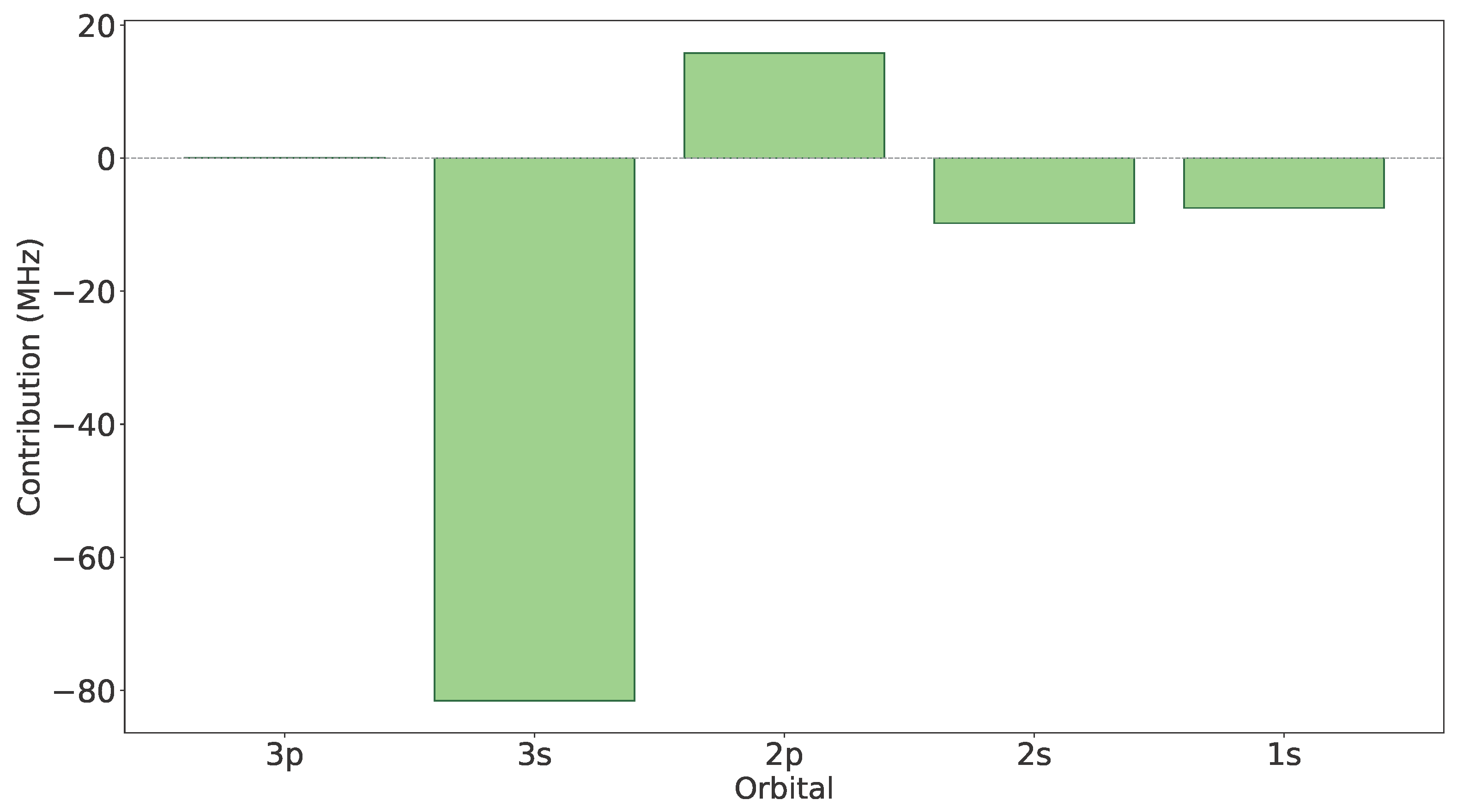
Figure 2.
Contributions of single (S) orbital substitutions relative to the DHF (left, in light green) and (right, in violet) constants in 43Ca II.
Figure 2.
Contributions of single (S) orbital substitutions relative to the DHF (left, in light green) and (right, in violet) constants in 43Ca II.
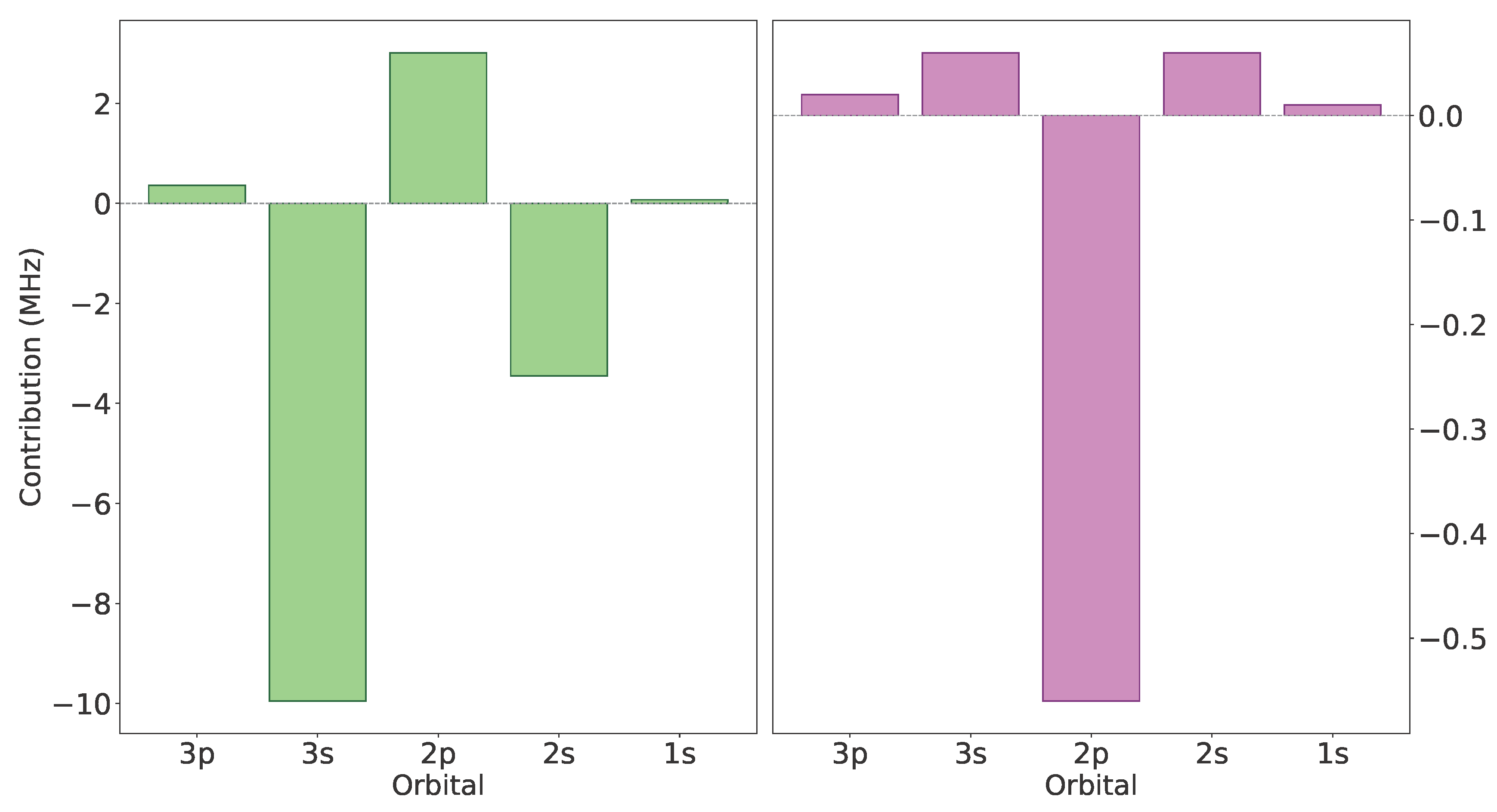
Figure 3.
Comparison between the large valence orbital component of the 43Ca II MCDHF CV SrD LBL calculation in solid blue, and multireference (MR) with allowed single (S) substitutions from all core orbitals transformed to natural orbitals (NO) in dashed red (top-left corner). The absolute difference given in green (bottom-left corner) shows the NO contraction in multiple areas between 0 and . A zoom is given on the right-hand side, showing more clearly the orbital contraction with the red arrow in the region.
Figure 3.
Comparison between the large valence orbital component of the 43Ca II MCDHF CV SrD LBL calculation in solid blue, and multireference (MR) with allowed single (S) substitutions from all core orbitals transformed to natural orbitals (NO) in dashed red (top-left corner). The absolute difference given in green (bottom-left corner) shows the NO contraction in multiple areas between 0 and . A zoom is given on the right-hand side, showing more clearly the orbital contraction with the red arrow in the region.
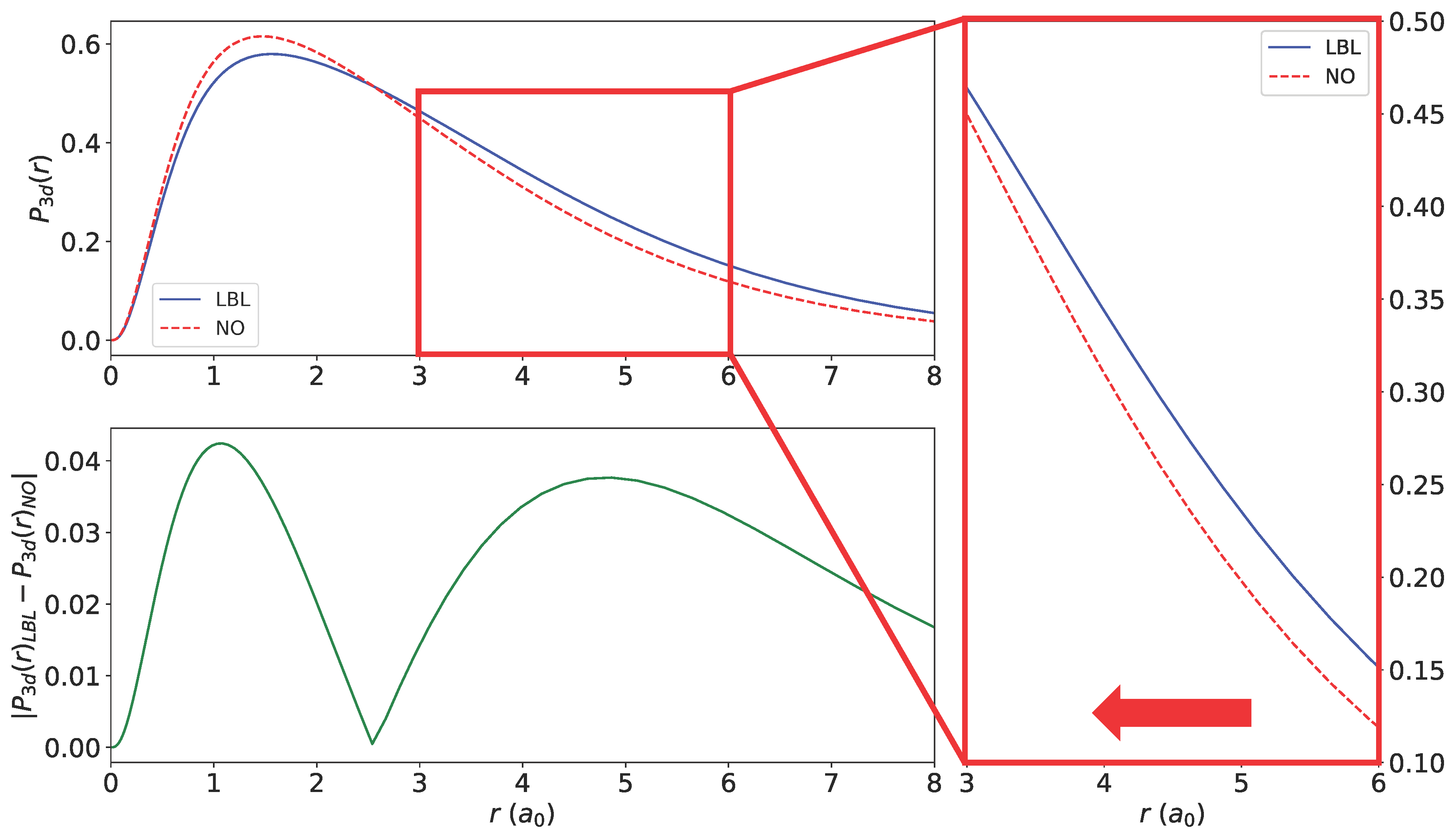
Figure 4.
Contributions of single (S) orbital substitutions relative to the DHF constant in 223Ra II.
Figure 4.
Contributions of single (S) orbital substitutions relative to the DHF constant in 223Ra II.
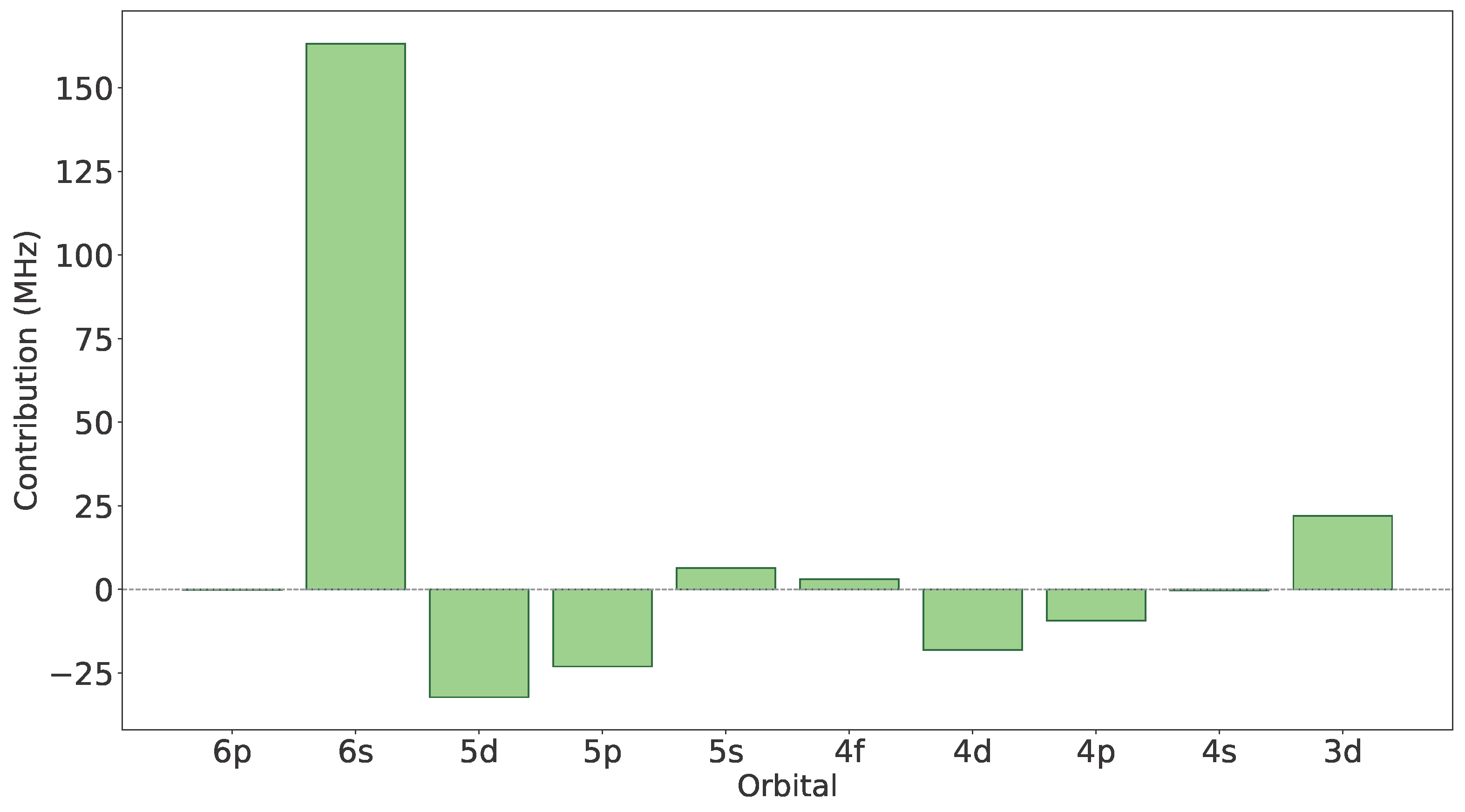
Table 1.
Considered active sets used for the levels studied in 43Ca II
| Correlation layer | 2 | 2 | 2 |
|---|---|---|---|
| DHF | |||
| AS1 | |||
| AS2 | |||
| AS3 | |||
| AS4 | |||
| AS5 | |||
| AS6 | |||
| AS7 |
Table 2.
Contributions from occupied orbitals to the calculated values of A hyperfine constant for the 2 level of 43Ca II. shows the individual contribution coming from the single (S) orbital substitutions.
Table 2.
Contributions from occupied orbitals to the calculated values of A hyperfine constant for the 2 level of 43Ca II. shows the individual contribution coming from the single (S) orbital substitutions.
| Orbital | A (MHz) | ||
|---|---|---|---|
| 1 | |||
| 32 | |||
| 2377 | |||
| 4303 | |||
| 12455 | |||
| 16468 |
Table 3.
Contributions from occupied orbitals to the calculated values of A and B hyperfine constants for the 2 level of 43Ca II. columns show the individual contribution to the HFS constant coming from the single (S) orbital substitutions.
Table 3.
Contributions from occupied orbitals to the calculated values of A and B hyperfine constants for the 2 level of 43Ca II. columns show the individual contribution to the HFS constant coming from the single (S) orbital substitutions.
| Orbital | A (MHz) | B (MHz) | |||
|---|---|---|---|---|---|
| 1 | −34.31 | −2.67 | |||
| 153 | −33.96 | +0.36 | −2.63 | +0.03 | |
| 8201 | −41.78 | −7.82 | −2.52 | +0.12 | |
| 14737 | −37.33 | +4.45 | −3.22 | +0.71 | |
| 44884 | −39.56 | −2.23 | −3.07 | +0.15 | |
| 58688 | −39.96 | −0.40 | −3.07 | +0.00 |
Table 4.
Comparison of (in ) and (in ) for the 2 levels of 43Ca II between layer-by-layer (LBL) (MCDHF CV ) and natural orbitals (NO) calculations. The spectroscopic orbital is highlighted in grey.
Table 4.
Comparison of (in ) and (in ) for the 2 levels of 43Ca II between layer-by-layer (LBL) (MCDHF CV ) and natural orbitals (NO) calculations. The spectroscopic orbital is highlighted in grey.
| Subshell | ||||
|---|---|---|---|---|
| LBL | NO | LBL | NO | |
| 2.5227 | 2.3033 | 0.5937 | 0.6947 | |
| 2.3718 | 2.3325 | 1.7532 | 1.5547 | |
| 2.4586 | 2.9116 | 2.4162 | 1.9883 | |
| 2.5629 | 3.0360 | 4.7478 | 5.5875 | |
| 3.0079 | 3.1761 | 6.3437 | 7.0810 | |
| 2.2484 | 3.8998 | 12.0424 | 5.4211 | |
| 5.2031 | 1.8125 | 2.4986 | 23.4276 | |
| 1.5182 | 5.1953 | 20.3480 | 6.1427 | |
Table 7.
Considered active sets used for the levels studied in 223Ra II.
| Correlation layer | 2 | 2 | 2 |
|---|---|---|---|
| DHF | |||
| AS1 | |||
| AS2 | |||
| AS3 | |||
| AS4 | |||
| AS5 | |||
| AS6 | |||
| AS7 |
Table 8.
Contributions from occupied orbitals to the calculated values of A hyperfine constant for the 2 level of 223Ra II. shows the individual contribution coming from the single (S) orbital substitutions.
Table 8.
Contributions from occupied orbitals to the calculated values of A hyperfine constant for the 2 level of 223Ra II. shows the individual contribution coming from the single (S) orbital substitutions.
| Orbital | A (MHz) | ||
|---|---|---|---|
| 1 | |||
| 33 | |||
| 3321 | |||
| 5914 | |||
| 25194 | |||
| 45642 | |||
| 54323 | |||
| 105167 | |||
| 163867 | |||
| 211495 | |||
| 229830 |
Table 9.
Magnetic dipole A hyperfine constant (in MHz) for 6d 2 in 223Ra II. The results at the top are from a HF calculation and the individual contributions from the orbital, spin-dipolar, and Fermi contact terms are shown along with the total value. The results at the bottom are the corresponding values from an MCHF calculation, including CV correlation based on one layer of correlation orbitals.
Table 9.
Magnetic dipole A hyperfine constant (in MHz) for 6d 2 in 223Ra II. The results at the top are from a HF calculation and the individual contributions from the orbital, spin-dipolar, and Fermi contact terms are shown along with the total value. The results at the bottom are the corresponding values from an MCHF calculation, including CV correlation based on one layer of correlation orbitals.
| Level | Term Contribution | |||
|---|---|---|---|---|
| Orbital | Spin-Dipolar | Contact | Total | |
| HF | ||||
| 2 | 46.42 | 15.49 | 0.0 | 61.91 |
| 2 | 30.95 | −4.43 | 0.0 | 26.52 |
| MCHF CV SrD | ||||
| 2 | 34.26 | 6.11 | 30.86 | 71.23 |
| 2 | 22.84 | −1.75 | −30.86 | −9.76 |
Table 11.
Bohr-Weisskopf (BW) corrected magnetic dipole A hyperfine structure constants (in MHz) of 223Ra II and 225Ra II and , respectively [48]), using the extracted relative BW corrections of Cserveny et al. [45], compared to available theoretical and experimental data. The recommended values are given in the form of , exhibiting a confidence level. a: Th. Sahoo et al. (RCC) [43]; b: Th. Cserveny et al. (AMPSCI) [45]; c: Th. Li et al. (RCC) [44]; d: Th. Pal et al. (SDpT) [46]; e: Th. Skripnikov et al. (RCC) [49]; f: Expt. Wendt et al. [41]; g: Expt. Neu et al. [42]
Table 11.
Bohr-Weisskopf (BW) corrected magnetic dipole A hyperfine structure constants (in MHz) of 223Ra II and 225Ra II and , respectively [48]), using the extracted relative BW corrections of Cserveny et al. [45], compared to available theoretical and experimental data. The recommended values are given in the form of , exhibiting a confidence level. a: Th. Sahoo et al. (RCC) [43]; b: Th. Cserveny et al. (AMPSCI) [45]; c: Th. Li et al. (RCC) [44]; d: Th. Pal et al. (SDpT) [46]; e: Th. Skripnikov et al. (RCC) [49]; f: Expt. Wendt et al. [41]; g: Expt. Neu et al. [42]
| Reference | 2 | 2 | 2 | 2 | 2 |
|---|---|---|---|---|---|
| 223Ra II | |||||
| This work (LBL) | 3,329 ± 359 | 68 ± 15 | −21 ± 4 | 603 ± 63 | 52 ± 4 |
| This work (NO) | 3,451 ± 331 | 72 ± 18 | −24 ± 4 | 640 ± 61 | 55 ± 3 |
| Th.a | 3,567 | 77 | -24 | ||
| Th.b | 3,424 ± 71 | 95 ± 20 | −29 ± 10 | 675 ± 13 | 57.7 ± 60 |
| Th.c | 3,426 ± 82 | 79.9 ± 1.7 | ± 2.3 | 660 ± 11.4 | 56.5 ± 1.2 |
| Th.d | 3,450 | 80 | -24 | 672 | 54 |
| Expt.f | 3,398.3 ± 2.9 | 667 ± 2.1 | |||
| Expt.g | 3,404 ± 1.9 | 56.5 ± 8 | |||
| 225Ra II | |||||
| This work (LBL) | −27,424 ± 3,038 | −560 ± 110 | 158 ± 37 | −4,984 ± 534 | −442 ± 24 |
| This work (NO) | −29,233 ± 4,193 | −612 ± 144 | 166 ± 37 | −5,478 ± 823 | −487 ± 59 |
| Th.a | −28,978 | −626 | 194 | ||
| Th.e | −27,731 | −5,451 | −461 | ||
| Expt.f | −5,446 ± 7 | ||||
| Expt.g | −27,731 ± 13 | −466.4 ± 4.6 | |||
Table 12.
Considered active sets used for the levels studied in 223Ra I.
| Correlation layer | 1 |
|---|---|
| DHF | |
| AS1 | |
| AS2 | |
| AS3 | |
| AS4 | |
| AS5 | |
| AS6 | |
| AS7 |
Table 13.
Magnetic dipole A and electric quadrupole B hyperfine structure constants (in MHz) of 223 [48]), compared to available theoretical and experimental data. The recommended values are given in the form of , exhibiting a confidence level. ★: Number of CSFs obtained after reduction using the rcsfginteract_csfg code; a: Th. Hassouneh et al. (MCDHF) [51]; b: Th. Bieroń et al. (MCDHF) [52]; c: Th. Calculated from Dzuba et al. (RHF+RCI) [53]; d: Expt. Lynch et al. [50]; e: Expt. Wendt et al. [41]
Table 13.
Magnetic dipole A and electric quadrupole B hyperfine structure constants (in MHz) of 223 [48]), compared to available theoretical and experimental data. The recommended values are given in the form of , exhibiting a confidence level. ★: Number of CSFs obtained after reduction using the rcsfginteract_csfg code; a: Th. Hassouneh et al. (MCDHF) [51]; b: Th. Bieroń et al. (MCDHF) [52]; c: Th. Calculated from Dzuba et al. (RHF+RCI) [53]; d: Expt. Lynch et al. [50]; e: Expt. Wendt et al. [41]
| Strategy | 3 | 3 | 1 | 3 | 3 | 1 | 3 | ||||||||||||
| Layer-by-layer (LBL) | |||||||||||||||||||
| MCDHF VV SrD | 626 | −458 | 91 | 910 | 292 | 135 | −81 | 303 | 898 | 350 | 199 | 635 | 896 | −323 | −225 | 228 | 852 | 565 | 425 |
| RCI CC SD | 85,320★ | −559 | 78 | 266,206★ | 272 | 133 | −75 | 272 | 189,081★ | 382 | 211 | 172,279★ | 963 | −322 | −219 | 353 | 320,622★ | 637 | 447 |
| RCI CC SD | 170,014★ | −567 | 98 | 531,502★ | 273 | 162 | −73 | 320 | 377,264★ | 388 | 264 | 353,923★ | 976 | −327 | −220 | 375 | 640,392★ | 646 | 459 |
| MCDHF VV SrD + CV SrD | 41,956 | −596 | 70 | 59,801 | 367 | 127 | −136 | 285 | 65,843 | 425 | 188 | 64,276 | 1,221 | −421 | −362 | 395 | 91,187 | 717 | 625 |
| RCI CC SD | 123,653★ | −572 | 79 | 322,284★ | 320 | 134 | −100 | 250 | 248,578★ | 404 | 209 | 237,283★ | 1,059 | −344 | −274 | 347 | 404,447★ | 666 | 477 |
| RCI CC SD | 208,347★ | −583 | 101 | 587,580★ | 320 | 166 | −98 | 302 | 436,761★ | 410 | 267 | 413,927★ | 1,070 | −345 | −274 | 371 | 724,217★ | 675 | 483 |
| MCDHF VV SrD + CV SrD | 116,496 | −658 | 129 | 167,242 | 421 | 212 | 212 | 396 | 186,546 | 477 | 328 | 177,207 | 1385 | −477 | −416 | 464 | 253,427 | 805 | 719 |
| RCI CC SD | 197,118★ | −623 | 129 | 429,417★ | 364 | 206 | −116 | 357 | 355,757★ | 447 | 330 | 349,045★ | 1,180 | −389 | −311 | 404 | 563,936★ | 735 | 548 |
| RCI CC SD | 280,602★ | −628 | 129 | 693,084★ | 362 | 204 | −113 | 343 | 553,300★ | 449 | 330 | 524,247★ | 1,179 | −372 | −309 | 397 | 881,802★ | 738 | 523 |
| Natural orbitals (NO) | |||||||||||||||||||
| MCDHF VV SrD | 626 | −458 | 91 | 910 | 292 | 135 | −81 | 303 | 898 | 350 | 199 | 635 | 896 | −323 | −225 | 228 | 852 | 565 | 425 |
| RCI CC SD | 85,320★ | −581 | 77 | 266,206★ | 280 | 134 | −76 | 278 | 189,081★ | 398 | 210 | 172,279★ | 1,000 | −384 | −202 | 444 | 320,622★ | 657 | 554 |
| RCI CC SD | 170,014★ | −607 | 112 | 531,502★ | 291 | 184 | −79 | 369 | 377,264★ | 416 | 298 | 353,923★ | 1,048 | −407 | −208 | 480 | 640,392★ | 691 | 600 |
| MCDHF VV SrD + CV SrD | 41,956 | −599 | 72 | 59,801 | 369 | 129 | −135 | 290 | 65,843 | 427 | 192 | 64,276 | 1,216 | −429 | −353 | 410 | 91,187 | 714 | 639 |
| RCI CC SD | 123,653★ | −595 | 80 | 322,284★ | 331 | 136 | −104 | 257 | 248,578★ | 420 | 212 | 237,283★ | 1,093 | −400 | −256 | 422 | 404,447★ | 686 | 569 |
| RCI CC SD | 208,347★ | −621 | 117 | 587,580★ | 342 | 189 | −107 | 354 | 436,761★ | 437 | 305 | 413,927★ | 1,138 | −421 | −262 | 480 | 724,217★ | 718 | 613 |
| MCDHF VV SrD + CV SrD | 116,496 | −664 | 132 | 167,242 | 425 | 216 | −157 | 403 | 186,546 | 481 | 334 | 177,207 | 1,377 | −492 | −400 | 494 | 253,427 | 800 | 746 |
| RCI CC SD | 197,118★ | −638 | 147 | 429,417★ | 374 | 231 | −119 | 409 | 355,757★ | 459 | 370 | 349,045★ | 1,202 | −458 | −284 | 505 | 563,936★ | 748 | 668 |
| RCI CC SD | 280,602★ | −662 | 147 | 693,084★ | 385 | 231 | −123 | 400 | 553,300★ | 474 | 370 | 524,247★ | 1,237 | −450 | −292 | 506 | 881,802★ | 776 | 658 |
| This work (LBL) | −593 ± 63 | 109 ± 35 | 318 ± 89 | 177 ± 46 | −95 ± 40 | 322 ± 41 | 416 ± 62 | 287 ± 74 | 1,075 ± 203 | −348 ± 45 | −267 ± 89 | 381 ± 28 | 686 ± 94 | 488 ± 65 | |||||
| This work (NO), recommended | −630 ± 57 | 125 ± 38 | 339 ± 94 | 201 ± 52 | −103 ± 45 | 374 ± 47 | 442 ± 59 | 324 ± 79 | 1,141 ± 189 | −426 ± 44 | −254 ± 85 | 489 ± 29 | 728 ± 87 | 624 ± 61 | |||||
| Th.a | −607 | 130 | 218 | 213 | −143 | 388 | 428 | 346 | 1,207 | −468 | −341 | 419 | 622 | 655 | |||||
| Th.b | −612 | 125 | 382 | 210 | −140 | 382 | 428 | 346 | 1,252 | −476 | −330 | 419 | |||||||
| Th.c | −604 | 257 | −47 | 403 | 1,185 | −242.3 | |||||||||||||
| Expt.d | 1,202.5 ± 3.0 | −472.1 ± 2.0 | |||||||||||||||||
| Expt.e | 1,202.1 ± 0.6 | −470.2 ± 1.2 | −344.5 ± 0.9 | 421.5 ± 1.6 | 699.6 ± 3.3 | 688.5 ± 4.0 | |||||||||||||
Table 14.
Bohr-Weisskopf (BW) corrected magnetic dipole A hyperfine structure constants (in MHz) of 223Ra I and 225Ra I and , respectively [48]), using the relative BW correction factor of Bieroń [52], i.e. 0.96, compared to available theoretical and experimental data. The recommended values are given in the form of , exhibiting a confidence level. a: Th. Hassouneh et al. (MCDHF) [51]; b: Th. Bieroń et al. (MCDHF) [52]; c: Th. Calculated from Dzuba et al. (RHF+RCI) [53]; d: Expt. Lynch et al. [50]; e: Expt. Wendt et al. [41]; f: Expt. Guest et al. [54]
Table 14.
Bohr-Weisskopf (BW) corrected magnetic dipole A hyperfine structure constants (in MHz) of 223Ra I and 225Ra I and , respectively [48]), using the relative BW correction factor of Bieroń [52], i.e. 0.96, compared to available theoretical and experimental data. The recommended values are given in the form of , exhibiting a confidence level. a: Th. Hassouneh et al. (MCDHF) [51]; b: Th. Bieroń et al. (MCDHF) [52]; c: Th. Calculated from Dzuba et al. (RHF+RCI) [53]; d: Expt. Lynch et al. [50]; e: Expt. Wendt et al. [41]; f: Expt. Guest et al. [54]
| Reference | 3 | 3 | 1 | 3 | 3 | 1 | 3 |
|---|---|---|---|---|---|---|---|
| 223Ra I | |||||||
| This work (LBL) | −569 ± 63 | 305 ± 89 | −91 ± 40 | 399 ± 62 | 1,032 ± 203 | −256 ± 89 | 659 ± 94 |
| This work (NO) | −605 ± 57 | 325 ± 94 | −99 ± 45 | 424 ± 59 | 1,095 ± 189 | −244 ± 85 | 699 ± 87 |
| Th.a | −607 | 218 | −143 | 428 | 1,207 | −341 | 622 |
| Th.b | −612 | 382 | −140 | 428 | 1,252 | −330 | |
| Th.c | −604 | 257 | −47 | 403 | 1,185 | −243.3 | |
| Expt.d | 1,202 ± 3.0 | ||||||
| Expt.e | 1,202.1 ± 0.6 | −344.5 ± 0.9 | 699.6 ± 3.3 | ||||
| 225Ra I | |||||||
| This work (LBL) | 4,654 ± 519 | −2,500 ± 726 | 743 ± 330 | −3,265 ± 509 | −8,439 ± 1,661 | 2,099 ± 730 | −5,388 ± 771 |
| This work (NO) | 4,946 ± 463 | −2,665 ± 767 | 808 ± 364 | −3,471 ± 482 | −8,957 ± 1,546 | 1,994 ± 692 | −5,717 ± 713 |
| Th.a | 4,905 | −1,763 | 1,153 | −3,455 | −9,751 | 2,757 | −5,027 |
| Th.b | 4,955 | −3,093 | 1,133 | −3,465 | −10,137 | 2,672 | |
| Th.c | 4,890 | −2,082 | 381 | −3,266 | −9,591 | 1,962 | −5,519 |
| Expt.f | 4,687.70 ± 1.5 | 2,796.5 ± 1.5 | |||||
| Expt.e | −9,793.9 ± 4.3 | ||||||
Disclaimer/Publisher’s Note: The statements, opinions and data contained in all publications are solely those of the individual author(s) and contributor(s) and not of MDPI and/or the editor(s). MDPI and/or the editor(s) disclaim responsibility for any injury to people or property resulting from any ideas, methods, instructions or products referred to in the content. |
© 2026 by the authors. Licensee MDPI, Basel, Switzerland. This article is an open access article distributed under the terms and conditions of the Creative Commons Attribution (CC BY) license (http://creativecommons.org/licenses/by/4.0/).
Copyright: This open access article is published under a Creative Commons CC BY 4.0 license, which permit the free download, distribution, and reuse, provided that the author and preprint are cited in any reuse.