

Submitted:
16 July 2026
Posted:
17 July 2026
You are already at the latest version
Abstract
Nuclear magnetic resonance (NMR) spectroscopy quantifies metabolites across many biological matrices, but in one-dimensional spectra of complex biofluids such as urine and plasma, extensive signal overlap obscures individual metabolite signals and complicates their quantification. Resolving these overlaps by deconvolution is only the first step: turning a set of spectra into a statistically analysable table also requires aligning corresponding signals across samples and condensing them into a feature matrix, a path that has typically been stitched together from several separate tools and is both cumbersome and time consuming. We present metabodeconplus, an R package that unifies this entire path into a single reproducible end-to-end workflow. From raw one-dimensional spectra, it deconvolutes overlapping signals as Lorentzian line shapes, automatically aligns the resulting peaks across samples, and condenses them into a data matrix of aligned signal integrals ready for built-in sample classification or downstream statistics. Automated parameter optimization removes manual tuning, and a Rust computational backend with parallelization reduces runtime substantially over the deconvolution-only predecessor MetaboDecon1D, from which the workflow is extended. The package is freely available as open source on GitHub and is currently under review at CRAN. metabodeconplus thus lowers the barrier from raw NMR spectra to reproducible metabolomic analysis.
Keywords:
1D NMR
; deconvolution
; metabolites
; quantification
; R package
; signal identification
1. Introduction
1.1. Background
Nuclear magnetic resonance (NMR) spectroscopy is a widely used analytical technique for detecting and quantifying metabolites in biological specimens such as urine, plasma, and tissue extracts [1]. By exploiting the magnetic properties of atomic nuclei, NMR provides structural and quantitative information about the molecular composition of a sample. Alongside mass spectrometry, this makes it a key tool in metabolomics, where researchers seek to characterize the metabolic profile of biological systems.
1.2. Challenges in 1D NMR Spectra Analysis
The goal of a metabolomics experiment is to identify and quantify the metabolites present in a sample. However, this information cannot be measured directly. Instead, certain chemical properties are recorded, allowing inferences about the contained metabolites. In NMR spectroscopy, the measured properties are the resonance frequencies of atomic nuclei in a magnetic field, which are influenced by their chemical environment, and the intensities at which those resonance frequencies appear. These resonance frequencies, often expressed as chemical shifts, together with their intensities act as a “fingerprint” that can be used to infer the presence and concentrations of specific metabolites [2]. However, despite its advantages, NMR spectroscopy faces challenges that complicate the direct extraction of metabolite concentrations from raw spectra. Two major issues that hinder accurate quantification are peak overlap and peak shifts.
1.2.1. Peak Overlap
Ideally, the resonance frequencies in an NMR spectrum would appear as sharp peaks, allowing straightforward identification and quantification. However, in reality, these peaks possess distinct linewidths and, therefore, may overlap with one another, making it difficult to distinguish individual signals. Several factors contribute to peak broadening, including T2 relaxation effects [3], magnetic field inhomogeneities [4], chemical exchange processes [5], sample viscosity, molecular interactions, which both contribute to relaxation [6], and the measurement process itself.
The process of reconstructing the individual metabolite contributions from a complex spectrum of overlapping peaks is known as deconvolution. This is one of the key challenges that metabodeconplus seeks to address.
1.2.2. Peak Shifts
Another major challenge in NMR-based metabolomics is that the resonance frequencies of the same metabolite do not always appear at exactly the same positions across samples. Several factors can cause these peak shifts, including variations in temperature [2], differences in sample pH [5], and variations in ionic strength and solvent composition [6].
These inconsistencies complicate direct comparisons between samples and hinder both identification and quantification of metabolites. To address this issue, signal alignment techniques are used to shift peaks across spectra to concordant positions, allowing for more accurate quantitative comparisons.
1.3. Existing Solutions
Available open-source solutions include the R packages BATMAN [7], rDolphin [8], Speaq 2.0 [9], ASICS [10], SigMa [11], and MetaboDecon1D [12] (the predecessor of this package), the Python program Decon1d [13], the MATLAB applications icoshift [14] and COW [15], and the web applications BAYESIL [16], DEEP Picker1D [17], and NMRProcFlow [18]. Proprietary software suites available for NMR spectral analysis include NMR Workbook Suite by ACD/Labs, AMIX by Bruker, Chenomx NMR Suite by Chenomx Inc., and MNova NMR by Mestralab Research. Furthermore, Bruker TopSpin 4.2 includes the program mldecon [19].
A summary of the main features of each tool is provided in Table 1; detailed descriptions of individual solutions are given in Appendix A.
1.4. The Role of Metabodeconplus
The aim of metabodeconplus is to deconvolute 1D NMR spectra of complex biofluids such as plasma, urine, or CSF that contain many overlapping peaks, in order to determine accurate integrals of the underlying peaks regardless of whether the corresponding metabolites are known. As a result, unidentified signals can also be used for classification tasks. We previously developed an R package for the deconvolution and integration of 1D NMR data (MetaboDecon1D [12]). This enabled the deconvolution of overlapping NMR signals. For each spectrum, the output is a list of deconvoluted signals characterized by their spectral positions together with accurate integral values. However, to make full use of these data, additional signal alignment is required for subsequent statistical analyses. metabodeconplus is not a new version of MetaboDecon1D but a new and substantially broader package: whereas MetaboDecon1D performed deconvolution of a single spectrum, metabodeconplus provides a complete, automated pipeline that takes a set of raw 1D NMR spectra all the way to an aligned, classification-ready table of signal integrals. First, the CluPA algorithm [20] of the speaq 2.0 package [9] was included. To this end, CluPA was adapted to the output format of MetaboDecon1D. The CluPA algorithm was chosen because it offers reliable alignment between target and reference spectra and has been implemented in R, which facilitated its addition to the metabodeconplus package. In addition, the underlying deconvolution algorithm was optimised for speed and accuracy.
The contribution of metabodeconplus is thus a single, automated end-to-end workflow for 1D NMR fingerprinting: from raw spectra it produces a two-dimensional table of aligned signal integrals that feeds directly into built-in sample classification. It achieves this by integrating three previously separate steps — deconvolution, peak alignment via the adapted CluPA algorithm, and classification — into one package, and by automating the parameter search these steps require. A substantially faster deconvolution backend makes the complete workflow practical on datasets of several hundred spectra. For a user, this means the entire path from raw spectra to a classification-ready feature matrix is handled by one package, replacing the ad-hoc combination of separate deconvolution and alignment tools that this analysis previously required.
2. Materials and Methods
2.1. Package Availability
The R package is available on GitHub at https://github.com/spang-lab/metabodeconplus and will be available on CRAN via https://cran.r-project.org/package=metabodeconplus.
2.2. Study Cohorts
Four datasets were used throughout this study. The Sim2 and Urine datasets are distributed with the package, whereas the Blood and AKI datasets can be obtained via download_example_datasets() or downloaded manually from GitHub.
The Sim2 dataset consists of 100 simulated spectra, each containing 2048 data points covering a chemical shift range of 3.59 to 3.28 ppm (datapoint spacing ppm). The spectra are evenly split into two groups, A and B (50 each). Each spectrum contains the same 25 underlying Lorentzian peaks: a fixed set of reference peak positions, peak intensities, and half-widths is reused across all spectra, with per-spectrum variability introduced by (i) a scalar global ppm shift drawn from ppm (sd datapoints), (ii) a per-peak ppm jitter drawn from ppm (sd datapoints), (iii) per-peak amplitude scaling drawn from , (iv) per-peak half-width scaling drawn from , and (v) additive Gaussian noise. In group A, the amplitudes of 3 of the 25 peaks (the discriminating peaks) are additionally scaled by fixed factors of , , and (); group B is left unmodified. The first spectrum is generated without any positional shift and serves as a clean unshifted reference. The shared reference parameters were derived from an initial deconvolution of the Blood dataset with manually optimized settings, so that the simulated spectra closely resemble real blood plasma spectra while providing exact ground truth for peak parameters, group labels, and noise levels.
The Blood dataset consists of 16 human blood plasma spectra measured with a 1D 1H Carr-Purcell-Meiboom-Gill (CPMG) pulse sequence.
The Urine dataset consists of 2 human urine spectra measured with a 1D 1H NOESY pulse sequence. Specimens from both the Blood and Urine data sets were obtained from specimens of the German Chronic Kidney Disease (GCKD) study collected at the baseline time point[21,22]. The GCKD study was carried out in accordance with the Declaration of Helsinki, registered in the German Register of Clinical Trials (DRKS 00003971), and approved by the ethics committees of the participating institutions.
The AKI dataset consists of 106 urinary 1D 1H NMR spectra acquired with a 1D 1H NOESY pulse sequence in the context of a study on acute kidney injury (AKI) following cardiac surgery with cardiopulmonary bypass (CPB) use [23]. Urinary specimens were collected 24 h after surgery. These spectra had been previously collected with written informed consent of the patients upon ethical approval from the University Clinic Erlangen, Erlangen, Germany. The study was approved by an institutional review board at the Faculty of Medicine at the Friedrich-Alexander-University (FAU) Erlangen-Nuremberg under the identifier #4010 [24].
All experimental measurements for these datasets were performed on a 600 MHz Bruker Avance III spectrometer (Bruker BioSpin GmbH, Rheinstetten, Germany) employing a helium cooled cryogenic probe and a cooled sample changer. The measurements were performed using optimized pulse sequences for the suppression of water signals.
An overview of all datasets is given in Table 2.
2.3. The Deconvolution Method
The deconvolution algorithm used in metabodeconplus was first described in Koh et al. (2009) and implemented as part of MetaboDecon1D v0.2.2 [12]. The implementation in metabodeconplus was completely restructured into a modular framework with four distinct stages: (i) smoothing, (ii) peak detection, (iii) peak filtering, and (iv) Lorentzian function fitting. A concise overview of the major functional differences between MetaboDecon1D v0.2.2 and metabodeconplus is provided in Table A1. The overall algorithm is visualized for a small, simulated spectrum in Figure 1.
2.3.1. Smoothing
Smoothing is required to suppress spurious detections caused by noise. Following Koh et al. (2009), we used a moving average filter with user-defined window size and iteration count before peak detection.
2.3.2. Peak Detection
Peak detection operates on the smoothed intensity vector using the curvature-based method introduced by Koh et al. (2009) [25]. Peaks are identified based on local minima in the second derivative of the signal. Each peak is represented by a left, center, and right point , with , respectively. Each peak is assigned the score introduced by Koh et al. (2009) [25]: , i.e. the smaller of the two cumulative absolute second-derivative sums over the peak’s left and right halves. Sharper, more prominent peaks therefore receive higher scores.
2.3.3. Peak Filtering
Peaks in the signal-free region are used to estimate the noise distribution. Only peaks with a score exceeding are retained, where and are the mean and standard deviation of the noise scores and is a user-tunable multiplier (default 6.4) that controls peak-detection sensitivity. Peaks inside user-specified ignore regions, such as the water-artifact region, are also removed.
2.3.4. Lorentzian Function Fitting
Each detected peak provides a triplet of observed points , , which uniquely determines the center , half-width , and amplitude A of a Lorentzian function passing exactly through those three points. These are the initial parameter estimates. When the resulting Lorentzian curves are superimposed, the sum tends to exceed the observed spectrum due to spill-over from neighboring peaks. Following Koh et al. [25], each peak’s height is, therefore, iteratively reduced by a rule of proportion until the superposition matches the raw spectrum. Compared to the original MetaboDecon1D implementation, metabodeconplus uses a more efficient strategy for computing the Lorentzian parameters during both initial estimation and iterative refinement; mathematical details are provided in Appendix C.
2.3.5. Rust Implementation
In addition to the native R implementation, metabodeconplus provides an optional Rust backend that implements the same deconvolution algorithm with further refinements for numerical stability and computational efficiency. The backend is accessible through the standard R interface via the use_rust parameter of deconvolute() and yields results that are numerically very close, though not identical, to the R implementation. The substantially reduced runtimes allow for a systematic grid search of optimal deconvolution parameters (Section 2.5.1) even for large datasets consisting of several hundred spectra.
2.3.6. Scoring of Deconvolution Quality
For scoring of deconvolution quality we devised a new measure called PRARPX, which scores both the number of correctly identified peaks and the approximation of the measured spectra. It is defined as , where the Extended Peak Ratio compares correctly identified peaks c to true peaks t plus incorrectly identified peaks i, and the Area Ratio is the total absolute residual R over the total absolute observed signal S. Both factors lie in and reach 1 only when the correct peaks have been recovered and the reconstruction matches the observed spectrum, so PRARPX approaches 1 for an ideal deconvolution. Because PRARPX requires ground-truth peak parameters, it is only applicable to simulated data or controlled measurements of known compounds; Appendix D motivates it in detail and contrasts it with using PR or AR alone.
2.4. The Alignment Method
Proper signal alignment is crucial to correct for chemical-shift variations across samples and to ensure that subsequent statistical analyses compare the same signals from the same metabolites. Following deconvolution, the obtained peak lists are passed through two consecutive steps: a coarse CluPA (cluster-based peak alignment) shift, followed by a refinement step snap_to_ref(). Both operate on the discrete peak grid: CluPA shifts whole spectrum segments by the same integer-datapoint offset, so all peaks within one segment move together — one peak may end up well-aligned while another in the same segment is still slightly off. The snap_to_ref() step removes this residual mismatch by snapping each remaining peak individually onto the nearest peak column of the reference spectrum. The two steps are exposed individually as clupa() and snap_to_ref() and are chained into a single call by the wrapper align(x, maxShift, maxCombine). The combined procedure is visualized for a set of simulated spectra in Figure 2.
2.4.1. CluPA
The first stage is based on the hierarchical cluster-based peak alignment (CluPA) approach from the speaq package [9,20]. CluPA aligns a target spectrum to a reference spectrum in two phases. First, it shifts the spectrum globally. Then, it iteratively splits the spectrum into smaller local segments that are individually aligned. The segment boundaries are defined by hierarchical clustering applied to the combined peak list of reference and target spectrum: peaks are grouped into a tree based on their distances, and at each iteration all segments are bisected according to the dendrogram. For each segment, the optimal integer datapoint shift is determined by fast Fourier transform cross-correlation, bounded by the user-supplied tolerance maxShift. Iterations stop when a segment contains only peaks from the same spectrum or fewer than three peaks. CluPA changes peak centers but does not change the number of peaks per spectrum.
2.4.2. snap_to_ref
CluPA shifts whole spectrum segments, not individual peaks, so peaks within the same segment all move equally in terms of direction and distance. Following CluPA, the alignment of spectra is substantially improved, but individual peaks are still not guaranteed to exhibit the exact same chemical shift across spectra, and a refinement step is needed to enforce a common peak grid. The snap_to_ref() step does this by collapsing (snapping) each spectrum’s peak list onto the peak grid of the reference spectrum chosen by CluPA. For each target peak, the nearest reference peak within maxCombine columns is its target; peaks farther than maxCombine from every reference peak are dropped. This may lead to the loss of rare peaks present in only few of the analyzed spectra and not in the reference spectrum. The interpretation of maxCombine is, therefore, the residual positional uncertainty that remains after CluPA. Figure 2 visualises the cumulative effect of the two steps: the top row overlays the six reconstructed spectra after each step, the middle row renders them as intensity heatmaps, and the bottom row reduces each spectrum to its sparse peak-position marks.
Both clupa() and snap_to_ref() align/snap each spectrum towards a fixed reference spectrum. This makes application to new samples trivial: each new sample is aligned and snapped to the same reference.
2.5. Parameter Optimization
2.5.1. Unsupervised Parameter Optimization
metabodeconplus’s deconvolution exposes four tunable parameters: nfit, smit, smws and delta. nfit sets the number of iterative Lorentzian-refinement passes, smit the number of moving-average smoothing passes, smws the smoothing window size (in datapoints), and delta the noise-threshold multiplier from Section 2.3.3. Without class labels, these can be optimized for each spectrum individually in an automated fashion by minimizing the area ratio (AR) between observed intensities and reconstructed intensities :
For evenly sampled spectra this is the mean absolute residual divided by the mean absolute signal, and smaller values indicate a better fit.
Minimizing the AR alone is not always optimal as the AR keeps decreasing as more Lorentzians are fitted, so the optimum may drift towards over-fit reconstructions with many spurious peaks. We, therefore, added as a user-defined parameter the maximum number of expected peaks npmax. The automated parameter optimization of the deconvolution step then sweeps a 60-cell parameter grid , , , and picks the smallest-AR cell whose peak count does not exceed npmax. As a consequence the user has to set only npmax manually. A suitable npmax can be set from domain knowledge (e.g., expected maximum peak numbers in blood or urine spectra) or chosen by maximizing downstream classification performance in case that class labels are available (Section 2.5.2).
The 60-cell grid above was chosen by deconvoluting representative blood and urine spectra over a broader candidate grid, visually inspecting the resulting Lorentzian reconstructions, and trimming the grid to the values that consistently produced plausible fits. The delta step of was picked so that the previous hand-tuned default falls on a grid point. Users who wish to use a finer control can pass an explicit deg argument.
2.5.2. Supervised Parameter Optimization
When class labels are available, npmax, maxShift and maxCombine can be optimized jointly by maximizing classification performance on the resulting feature matrix. Because the same metabolites may not be present in all spectra, zeros in the feature matrix encode “missing peak” rather than “zero area”. Linear models confound these zeros with small observed values and become unstable; we therefore use a non-linear random forest classifier from the ranger package [26], which can partition on presence as well as magnitude. A further advantage of random forests is the out-of-bag (OOB) error [27], a generalization-error estimate obtained during training itself, which we use as our score without an extra held-out split or inner cross-validation loop.
The two alignment parameters — maxShift (CluPA tolerance) and maxCombine (snap-to-ref window width) — are governed by different sources of positional error and their empirical optima do not necessarily coincide, so tuning them jointly is in general not redundant. All three parameters can therefore in principle be swept as a three-dimensional grid via the supervised search in fit_mdm().
In practice, we do not recommend tuning all three at once: the runtime grows multiplicatively with the size of each axis, and the deconvolution and CluPA stages dominate that cost. We instead recommend the following two-step procedure:
- 1.
- Pick npmax from domain knowledge (e.g., urine spectra typically contain more metabolites than blood) or by visual inspection of a representative deconvolution, as in Section 2.5.1.
- 2.
- Rely on CluPA’s internal optimum by passing the sentinel maxShift = -1. This sentinel triggers an adaptive sweep that doubles maxShift through , runs CluPA at each step, computes the average pairwise Pearson correlation of the aligned Lorentzian superpositions, and stops one step before that correlation first decreases.
The supervised search is then reduced to a one-dimensional sweep over maxCombine, which is by far the cheapest of the three stages to rerun.
fit_mdm() relies on caching and multiprocessing to keep its runtime reasonable. Three optimizations are combined:
- 1.
- Each npmax value has an associated set of per-spectrum deconvolution parameters that give the lowest reconstruction error. Finding them requires an internal grid search per spectrum, which is run once at function entry and attached to each spectrum. Whenever npmax changes the optimal parameters can be looked up instead of repeatedly recomputed.
- 2.
- The grid is traversed in (npmax, maxShift, maxCombine) order, so npmax varies slowest. If npmax is unchanged between two rows, the deconvolution of the previous row is reused instead of recomputed; if npmax and maxShift are both unchanged, the CluPA alignment is reused as well.
- 3.
- Deconvolution, alignment and fitting each use several workers. We parallelize over spectra rather than over grid rows to keep memory low: parallelizing over grid rows would force every worker to hold a copy of all spectra, whereas parallelizing over spectra means each worker only holds the spectra it is currently processing.
3. Results
3.1. Deconvolution Quality on Sim2: Metabodeconplus vs. MetaboDecon1D and Grid Search
The evaluations that follow quantify the payoff of the integrated metabodeconplus workflow for the user: automatically tuned deconvolution and alignment, fast enough to scale to hundreds of spectra, at no cost in downstream classification performance. We scored deconvolution quality with PRARPX as defined in the materials and methods section. To this end, we devised a simulated dataset Sim2 (see Table 2 for details). Note that this simulated dataset also contained noise to approximate a realistic experimental data set. Figure A2 shows an example spectrum of this data set. Each of the 100 Sim2 spectra was deconvoluted with MetaboDecon1D (default parameters), metabodeconplus (default parameters), and metabodeconplus with unsupervised grid-search parameter selection at . The signal-free region was auto-derived per spectrum so that all methods saw equivalent inputs. Note that PRARPX is computed from ground-truth peak parameters, whereas the general grid search parameter optimization has to operate on the area-ratio alone. Therefore, a PRARPX of 1 is unreachable in practice.
Table 3 summarises PRARPX (mean, sd, min, max) across all spectra for each configuration, and Figure 3 plots the per-spectrum trace. The default metabodeconplus configuration already improved on MetaboDecon1D, and the grid-search cutoff at moderate npmax closed most of the remaining gap to the metabodeconplus optimal bound.
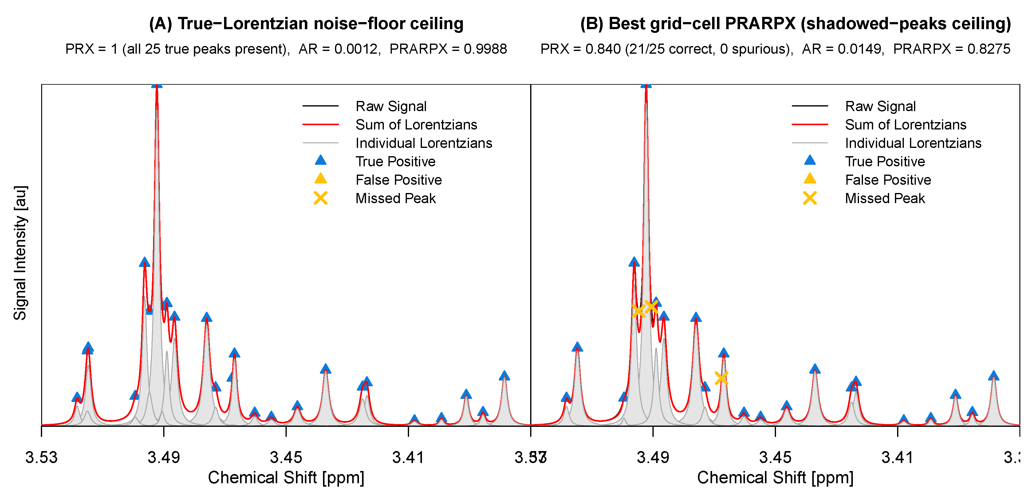
Even with the metabodeconplus optimal parameters an ideal value of is not reached for two reasons. First, the superposition of the estimated noiseless Lorentzian signals cannot fully reproduce the noisy observation. Figure A2A illustrates this. Second, small peaks completely shadowed by larger neighbours produce no detectable curvature minimum and are therefore not recovered, so for ordinary spectra (Figure A2B).
3.2. Alignment Quality on Sim2: CluPA and snap_to_ref
To quantify alignment quality directly we exploited the fact that every Sim2 spectrum contains the same 25 simulated peaks named A–Y at known positions, with the first spectrum simulated without any per-spectrum jitter or global shift so that it serves as the unshifted reference. For each extracted peak we recorded to which of these 25 simulated peaks it corresponded to: a peak whose fitted center lay within data points of a simulated position inherited that peak’s name; a peak farther away from any simulated position was labeled Z (a spurious detection). Labels are assigned to the raw deconvolution output, before any alignment, so each peak carries the identity of the simulated source it came from through the rest of the pipeline.
After CluPA each peak is potentially shifted but still positioned on the continuous chemical-shift axis. The snap_to_ref() step then collapses these onto the discrete peak grid of the unshifted reference spectrum: each peak is moved to the nearest reference column within a snap window of maxCombine datapoints, and peaks outside of this window are dropped. With labels in hand we asked, for each spectrum and each true-peak, whether the reference column belonging to a certain peak ended up populated by the right peak. The fraction of correct pairs over the full grid is the snap purity reported in Figure 4.
Results show that the snap purity is highest where CluPA has already brought peaks within a small maxCombine window of their reference columns. On Sim2 the maxCombine axis shows no valley because the 25 simulated peaks are spaced far enough apart (tens of data points) that even the widest snap windows rarely sweep in a wrong neighbour; on a more crowded spectrum, widening maxCombine past the optimum would start trading correct snaps for wrong-label intrusions and a clear valley would appear (data not shown).
3.3. Supervised Parameter Optimization on Sim2
In the following, it is demonstrated that the supervised search described in Section 2.5.2 where class labels are known is feasible. To this end, we ran a 5000-tree ranger probability forest over a small grid. The grid spans all three parameters (, , ). This Sim2 sweep is the only instance where all three parameters were tuned at once: the small spectrum count and coarse grid keep the runtime under a few minutes. This allowed to analyze whether the supervised optimum of parameters obtained here is consistent with the unsupervised one. The grid search selected , , as the best combination (OOB accuracy , OOB AUC ). Applied to the held-out 50 test spectra, this configuration achieved a test accuracy of and AUC of . Of the top-10 features ranked by ranger permutation importance, 3 fall within 3 datapoints of a discriminative peak.
The supervised optimum coincides with the unsupervised optimum of Section 3.1. All three discriminating peak positions are recovered in most spectra. Note, the supervised search optimises classification accuracy rather than reconstruction fidelity as in the unsupervised search, so the two criteria need not select the same in general; in contexts where peak recovery rather than classification accuracy is the criterion of interest, is more naturally set to a prior upper bound on the expected peak count than tuned by the supervised search.
The out-of-bag (OOB)-AUC and OOB-accuracy heatmaps obtained for the different parameter combinations are shown in Figure 5 a and b, respectively. A heatmap of all features selected in the training data set by the ranger classification (Figure 5 c). Data are shown for the optimal set of parameters obtained in the supervised search. Each column is labeled with its corresponding chemical shift position in ppm. Columns to the left of the center are features whose mean is higher in Group A (positive two-sample t-score) and vice versa for columns to the right. Within each half , columns are sorted by ranger feature importance [26,27] so that the most informative features are located at the left or right borders of the plot. A feature is counted as matching a discriminative peak when its center lies within data points of one of the 3 discriminatory peaks. Figure 5 d shows a superposition of 5 group-A and 5 group-B training spectra after alignment and snapping, zoomed on the range of ranger features (plus ppm of padding), with one vertical line per feature shown in (c). Green lines mark features within datapoints of a discriminative peak.
Data show that good classification performance is obtained with automated parameter optimization. As can be seen from Figure 5 a and b classification performance is relatively robust with respect to parameter settings with a broad maximum in the parameter matrix. Figure 5 c shows that the true discriminatory features are amongst the most informative features picked by the classification algorithm. That also other features are considered by the classification algorithm is due to the fact that the three discriminatory features of group A were up and down scaled only very moderately. Furthermore, a per-peak amplitude scaling and the addition of Gaussian noise were performed on the Sim2 data set as described in the Study cohorts section. As can be seen from Figure 5 d the three discriminatory peaks are of only moderate intensity and show partial overlap with other signals. Therefore, the Sim2 data set provides a challenging realistic example.
3.4. End-to-End Prediction Performance on the AKI Dataset
We evaluated end-to-end predictive performance on the AKI dataset (34 AKI versus 72 control urinary spectra, creatinine-normalised) by comparing two models. The first was an equidistant-binning baseline that mirrors the fixed-bin feature representation originally used by Zacharias et al. [23], who introduced the AKI dataset: a 700-bin feature matrix consisting of 300 bins covering – ppm and 400 bins covering – ppm (a fixed bin width of ppm). Whereas Zacharias et al. [23] classified these features with a support-vector machine (SVM), we replaced the SVM with a ranger-based random forest [26,27,28] run in probability mode (one class probability per sample), matching the classifier used by the metabodeconplus pipeline and ensuring a fair comparison. The second was the full metabodeconplus pipeline: deconvolute → CluPA → snap_to_ref → ranger, with fixed.
Following the recommendation of Section 2.5.2, we fix on the AKI dataset rather than tuning it. The choice was made by visual inspection of the deconvolution output on the two Urine spectra introduced in Table 2: at , the fitted Lorentzian superposition reconstructs every visually-resolvable peak of those reference urine spectra while keeping the residual free of obvious unfit signal, so the same setting was expected to be a sensible default for the AKI urine cohort, which was acquired with the same NMR pulse sequence. We further rely on CluPA’s internal optimum for by passing the sentinel (see Section 2.5.2), so that only is swept on the training fold of each cross-validation split via the inner grid-search in fit_mdm().
Predictive performance was estimated by stratified 10-fold cross-validation repeated over three random seeds (so 30 folds in total per model). Each fold’s training portion was independently re-fit before scoring on the held-out fold, and standard errors are taken across folds. The binning baseline reached % accuracy and ; metabodeconplus reached % and , thus matching the binning baseline with no loss in accuracy or AUC, while operating on a higher-resolution feature matrix whose columns correspond to individually localised peaks rather than fixed-width bins.
To compare what the two models had learnt, we refitted both on the full AKI dataset, extracted ranger permutation importances, and overlaid the top 20 features of each model on the alignment reference spectrum across the – ppm aliphatic region (Figure 6).
On its higher-resolution, per-peak feature matrix, metabodeconplus performed on par with the binning model. One main advantage of using a deconvolution approach is that each selected feature is a single deconvoluted peak that contributes to only one metabolite. This allows for an unambiguous metabolite assignment of selected features. This is of special importance in case the measurement of predictive signatures should be transferred to other methods from, for example, clinical chemistry. In addition, this allows for a biological interpretation of obtained signatures. In this context it should be noted that predictive signatures only provide correlations between metabolites and groups of specimens; they do not provide causal relationships. Whereas, as can be seen from Figure 6, for the binning model a bin may contain contributions from multiple peaks and metabolites, which substantially hinders assignment of predictive signatures to corresponding metabolites.
3.5. Runtime Performance and Parallel Scaling
We compared the per-spectrum, single-core runtime of the original MetaboDecon1D implementation (Figure 7 A), the R implementation of the new metabodeconplus package (Figure 7 B), and the Rust backend of metabodeconplus as activated from within the R environment (Figure 7 C). To this end, spectra with different numbers of data points ( to ) and peak counts ( to ) were simulated. Typical 1D 1H spectra of biofluids such as urine and plasma consist of to data points with approximately 1000 peaks. For the original MetaboDecon1D implementation, this resulted in an average runtime of around 40 s at data points (Figure 7 A). In the R implementation of the new metabodeconplus package, the runtime is substantially reduced to well below one second per spectrum in this regime (Figure 7B). The Rust backend (Figure 7 C) provides a further speed-up that becomes most pronounced for densely-peaked spectra: at data points and 4096 peaks the deconvolution takes around s in pure R but only around s with Rust, while at the more typical peaks the two backends are essentially indistinguishable on a single spectrum. Panels A–C of Figure 7 are single-core single-spectrum measurements; parallelisation across spectra is shown separately in Figure 7 D showing the deconvolution times of all 106 AKI spectra with respect to the degree of parallelization () for both the R and Rust backend. Runtime scales close to the ideal reference throughout the measured range, with the Rust backend completing the full 106-spectrum batch in under 6 s at and the R implementation in under 8 s. These short runtimes make it tractable to determine the optimal deconvolution parameters for each dataset individually by systematic grid search.
4. Discussion
With metabodeconplus we provide a single end-to-end workflow for the analysis of 1D NMR fingerprinting data of complex biofluids, requiring no prior knowledge of the individual molecules present. The workflow integrates three steps that previously required separate tools: deconvolution of overlapping signals into individual Lorentzian lines, alignment of the deconvoluted peaks, and sample classification, tied together by an automated parameter search. Results showed that, with the new implementation of the deconvolution algorithm, a substantial improvement in runtime could be obtained. With this the deconvolution of large datasets containing several hundreds of spectra becomes feasible. This is especially true when the Rust implementation of the deconvolution part is used. This substantial improvement in runtime permits a systematic search of optimal deconvolution and alignment parameters. To analyze the performance of metabodeconplus in terms of peak detection and deconvolution, a carefully designed challenging simulated data set was used, where the ground truth is known. We could show that metabodeconplus facilitates a reliable peak detection and deconvolution of overlapping signals in complex data. The residual gap to on the simulated data is dominated by the additive-noise floor (raising AR above zero) and by small peaks shadowed by larger neighbours (suppressing PRX), as detailed in Section 3.1 and illustrated in Figure A2. Deconvolution quality depends on appropriate parameter selection. We devised a grid search procedure to search parameter space by optimizing the area ratio. However, especially for complex experimental spectra it is not guaranteed that this will always lead to an optimal selection. One critical parameter is the expected maximal number of peaks npmax that ensures that not a large number of spurious signals is detected. For experimental data such as urine and plasma spectra we recommend setting the the maximum number of expected peaks based on prior knowledge e.g. to 1000 for human urine. To make full use of the deconvoluted data in subsequent statistical analysis proper peak alignment is required to correct for small variations in peak positions across spectra. We employ the well established CluPA algorithm that was extended by the snap_to_ref function to ensure that corresponding peaks are put to the exact same position. As we could show, this in general provides a good alignment. However, alignment quality depends on the two parameters maxShift and maxCombine. The parameters npmax, maxShift and maxCombine may be manually set by the user after careful spectra inspection. We also devised an automated supervised grid search via fit_mdm() that can in principle tune all three jointly when two well-separable classes with known class labels are available. In practice we recommend, as mentioned above, fixing npmax from domain knowledge or visual inspection, leaving maxShift to the adaptive CluPA-internal sweep selected by maxShift = -1, and tuning only maxCombine on the labelled data — this avoids the multiplicative runtime of the full three-dimensional grid without sacrificing classification performance. The higher spectral resolution and interpretability of the peak-based feature matrix were achieved without loss of predictive performance: classification matched the equidistant-binning baseline, while each discriminatory feature could be assigned to an individual metabolite — which a coarse bin, mixing several peaks, does not permit. In summary, metabodeconplus makes 1D NMR fingerprinting a single automated workflow — from deconvolution through alignment to classification — with automated parameter optimization and a fast, parallelised backend that make this end-to-end pipeline practical at the scale of modern metabolomics cohorts.
Limitations Direct file-format support is restricted to Bruker and JCAMP-DX; other vendor formats are not parsed natively. Users can however hand spectra in as a chemical-shift vector and a corresponding signal-intensity vector, so any format that can be loaded into the R session is usable. Native readers for further vendor formats remain future work. No routines are provided to group deconvoluted peaks into multiplet structures, and no automatic peak-to-metabolite assignment (e.g. matching against reference spectra) is included. Finally, PRARPX has a hard upper bound below 1 on noisy spectra: additive measurement noise keeps and peaks completely overlapped by larger neighbours produce no detectable curvature minimum and are therefore not recovered (Figure A2).
Author Contributions
Conceptualization, W.G. and T.S.; methodology, T.S., M.S., and W.G.; software, T.S. M.S., and W.G.; investigation, W.G.; resources, P.J.O., R.S. and W.G.; data curation, H.U.Z., and W.G.; writing—original draft preparation, T.S.; writing—review and editing, T.S., M.S., P.J.O., R.S. and W.G. All authors have read and agreed to the published version of the manuscript.
Funding
The authors acknowledge the support from the Deutsche Forschungsgemeinschaft (DFG, German Research Foundation), project number 509149993, TRR374.
Institutional Review Board Statement
The urine AKI data set originated from a study on acute kidney injury (AKI) after cardiac surgery [23]. The AKI study was approved by the local Institutional Review Board (Ethik-Kommission der Medizinischen Fakultät der Friedrich-Alexander-Universität Erlangen-Nürnberg, #4010), reference: https://doi.org/10.1371/journal.pone.0145042. Further urine and plasma specimens were obtained from the German Chronic Kidney Disease (GCKD) study. The study was carried out in accordance with the Declaration of Helsinki, registered in the German Register of Clinical Trials (DRKS 00003971), and approved by the ethics committees of the participating institutions.
Informed Consent Statement
Informed consent was obtained from all subjects involved in the study.
Data Availability Statement
Publicly available datasets were analyzed in this study. All datasets are available from the metabodeconplus GitHub repository at https://github.com/spang-lab/metabodeconplus. The urinary AKI dataset has also been uploaded to the publicly available MetaboLights database, identifier: MTBLS24. The GCKD plasma spectra are also available from the MetaboLights database, identifier: MTBLS798.
Acknowledgments
We thank all the GCKD study participants for their time and important contributions, all participating nephrologists’ practices and outpatient clinics for their continued support, as well as the GCKD study personnel and investigators for their enormous commitment. We would also like to thank all GCKD investigators, which are as follows: Kai-Uwe Eckardt, Heike Meiselbach, Markus P. Schneider, Mario Schiffer, Hans-Ulrich Prokosch, Barbara Bärthlein, Andreas Beck, Andre´ Reis, Arif B. Ekici, Susanne Becker, Ulrike Alberth-Schmidt, Anke Weigel, Sabine Marschall, Gerd Walz, Anna Köttgen, Ulla T. Schultheiß, Fruzsina Kotsis, Simone Meder, Erna Mitsch, Ursula Reinhard, Jürgen Floege, Rafael Kramann, Turgay Saritas, Elke Schaeffner, Seema Baid-Agrawal, Kerstin Theisen, Kai Schmidt-Ott, Martin Zeier, Claudia Sommerer, Mehtap Aykac, Gunter Wolf, Martin Busch, Andy Steiner, Thomas Sitter, Christoph Wanner, Vera Krane, Britta Bauer, Florian Kronenberg, Barbara Kollerits, Lukas Forer, Julia Raschenberger, Sebastian Schönherr, Hansi Weissensteiner, Peter J. Oefner, Wolfram Gronwald, Matthias Schmid, and Jennifer Nadal.
Conflicts of Interest
The authors declare no conflict of interest. The funders had no role in the design of the study; in the collection, analyses, or interpretation of data; in the writing of the manuscript, or in the decision to publish the results. The authors declare that they used large language models to improve the English of the manuscript.
Abbreviations
The following abbreviations are used in this manuscript:
| 1D | one-dimensional |
| CPMG | Carr-Purcell-Meiboom-Gill |
| FA | formic acid |
| HSQC | heteronuclear single quantum coherence |
| NMR | nuclear magnetic resonance |
| TSP | trimethylsilylpropanoic acid |
Appendix A. Existing Solutions for NMR Spectra Analysis
- ACD/NMR Workbook Suite by ACD/Labs is a commercial software suite for NMR data processing. It includes spectral deconvolution, metabolite quantification, and statistical analysis capabilities, but the underlying algorithms are proprietary and not publicly disclosed.
- AMIX by Bruker is a commercial software suite for NMR-based metabolomics. It supports spectral processing, bucketing, and statistical analysis, but its deconvolution and alignment algorithms are proprietary.
- Chenomx NMR Suite by Chenomx Inc is a commercial software suite combining spectral deconvolution and library-based metabolite identification and quantification. Implementation details are not publicly available.
- MNova NMR by Mestralab Research is a commercial software suite for NMR data processing, offering deconvolution, quantification, and statistical analysis. Its algorithms are proprietary.
- MetaboLab by Ludwig and Günther, 2012, is a MATLAB-based software for NMR data processing offering algorithms for baseline correction and alignment via a graphical user interface. The software appears to no longer be actively maintained.
- BATMAN by Hao et al., 2012, uses Bayesian modeling and Markov-Chain Monte Carlo (MCMC) together with spectral libraries for automated metabolite quantification in 1D NMR spectra. It incorporates prior peak information and handles overlaps and baseline distortions, but requires careful tuning and substantial computational resources.
- Bayesil by Ravanbakhsh et al., 2015, is a fully automated web system for rapid NMR spectral profiling. Given a 1D 1H NMR spectrum of a complex biofluid, it autonomously identifies and quantifies metabolites with high accuracy using Bayesian spectral fitting against a reference library.
- Icoshift by Savorani et al., 2010, is a MATLAB application for alignment of 1D NMR spectra. It optimizes the cross-correlation between user-defined intervals of a target and a reference spectrum to correct chemical-shift variations. SigMa [11] uses a modified version of the icoshift algorithm for its alignment step.
- COW (Correlation Optimized Warping) by Tomasi et al., 2004, is a MATLAB application for chromatographic and spectroscopic data alignment. It divides the spectrum into segments and uses dynamic programming to maximize the segment-wise cross-correlation between a sample and a reference, allowing non-linear warping of the chemical-shift axis.
- Decon1d by Hughes et al., 2015, is a Python script for deconvoluting 1D NMR spectra, originally developed for 19F spectra of labeled proteins. It iteratively places peaks using the Levenberg–Marquardt algorithm and selects the most parsimonious model via the Bayesian Information Criterion (BIC).
- NMRProcFlow by Jacob et al., 2017, is a graphical and interactive web application for preprocessing 1D NMR spectra, covering baseline correction, alignment, and bucketing. It does not include a dedicated signal deconvolution algorithm but applies a Least-Squares approach for alignment of user-defined intervals.
- AQuA by Rohnisch et al., 2018, is a software tool for automated quantification of metabolites in 1D NMR spectra, addressing peak overlap and baseline distortions.
- rDolphin by Canueto et al., 2018, is an R package for analysis of 1D NMR spectra that combines spectral library fitting for metabolite quantification with interactive optimization capabilities.
- ASICS by Lefort et al., 2019, is an R package providing a complete workflow for 1D 1H NMR spectra. For quantification, it first aligns selected library spectra with the sample spectrum, then fits the aligned library spectra using a sparse model.
- NMRbox is a web platform offering virtual machines with a broad collection of NMR software tools. It does not provide its own standalone deconvolution or alignment algorithm.
- Speaq 2.0 by Beirnaert et al., 2018, is an R package for high-throughput processing of 1D NMR spectra. Signals are first represented as wavelets and then aligned across spectra using the hierarchical CluPA algorithm [20], yielding a two-dimensional feature matrix suitable for downstream statistical analysis with tools such as MetaboAnalyst [29].
- SigMa by Khakimov et al., 2020, is a fully automated approach for quantification of 1D 1H NMR metabolomics data, particularly from human urine. It combines peak picking, a modified icoshift alignment, and signal deconvolution, and explicitly discriminates between signals matching known reference metabolites and unassigned spectral regions.
- MetaboDecon1D by Hackl et al., 2021, is an R package for automatic deconvolution of 1D NMR spectra into Lorentzian curves using a curvature-based peak-detection algorithm. It is the direct predecessor of metabodeconplus.
- DEEP Picker1D by Li et al., 2023, is a convolutional neural network trained on synthetic 1D NMR spectra for peak detection and parameter estimation. Predicted peak parameters are refined by a Voigt fitter via nonlinear least squares, yielding a full quantitative representation of the spectrum.
- mldecon by Schmid et al., 2023, is a deep learning-based deconvolution command available in Bruker TopSpin 4.2. Trained on synthetic spectra, it accurately estimates peak parameters and performs well on crowded, high-dynamic-range, and shoulder-peak regions.
Appendix B. Major Differences Between the Current Version and MetaboDecon1D

Table A1.
Concise comparison of major functional differences between MetaboDecon1D and metabodeconplus
Table A1.
Concise comparison of major functional differences between MetaboDecon1D and metabodeconplus
| Aspect | MetaboDecon1D | metabodeconplus |
|---|---|---|
| Scope | Deconvolution | Deconvolution, Alignment, Modelling |
| Implemented in | R | R and Rust |
| Peak fitting | Uses original formulation | Uses algebraically simplified equations |
| Smoothing | Smoothed intensities propagate into fitting | Smoothing is used for peak detection only; Lorentzian fitting uses the raw intensities |
| Artifact handling | Negative intensities rectified; water region set to zero | Negative intensities retained; user-defined ignore regions replace hard zeroing of artifact regions |
| Parameter optimization | Manual parameter selection | Manual selection or grid search via npmax |
| Alignment | Not available | CluPA followed by snap_to_ref |
| Predictive modelling | Not available | End-to-end classifier pipeline via fit_mdm() with a Random Forest learner; nested-CV performance estimation via benchmark() |
| Performance and reuse | Legacy implementation | Faster peak detection and smoothing, parallel execution, and optimized Lorentzian superposition |
Appendix C. Mathematical Details of Lorentzian Function Fitting
The Lorentzian function, also known as the probability density function of the Cauchy distribution, is defined as:
where is the center and is the half-width at half-maximum. Since the integral is normalized to 1, an additional amplitude factor A replaces the normalization term :
For each detected peak, a stencil of three observed points , , gives the system:
Eliminating A and yields a closed-form expression for :
With known, the product can be isolated:
Comparing any two instances of Equation (A5) gives an expression for :
Using the outer pair directly causes numerical instability because quasi-symmetric peaks have . Instead, and are computed and averaged:
The product is then obtained from the central point :
Note that together with and is sufficient to evaluate the Lorentzian at any without resolving A and separately.
After computing initial estimates for all peaks, the superposition is compared to the raw unsmoothed intensities. Following Koh et al. [25], the intensity stencils of each peak are rescaled by the ratio of observed to reconstructed intensity (rule of proportion), and the fitting step is repeated. This iterative refinement continues for a user-defined number of iterations (nfit).
In the original MetaboDecon1D implementation [12], smoothed intensities were used for both peak detection and fitting. Smoothing disproportionately reduces the apparent height and width of narrow peaks, biasing the parameter estimates. metabodeconplus uses smoothed intensities only for peak detection and fits Lorentzian parameters to the raw intensities, reducing this systematic bias. Additionally, estimated A and values below a multiple of machine precision are discarded at the end of refinement to suppress numerical artifacts.
Appendix D. The PRARPX Metric
Common methods for assessing deconvolution quality include evaluation of the Area Ratio (AR), evaluation of the Peak Ratio (PR), i.e., comparing the number of detected peaks to the true number of peaks, and visual inspection. However, all of these methods have limitations. Residual-only criteria such as the AR tend to improve with the number of detected peaks, regardless of the true number of peaks. Finding the correct number of peaks does not necessarily mean that the correct peak parameters have been found. Additionally, in real-world applications, the true number of peaks is typically unknown. Visual inspection is subjective and not suitable for large datasets. To address these issues, we developed PRARPX for evaluating deconvolution quality when true signals are known, as is the case for simulated data or real samples with spiked-in controls. PRARPX combines features of the above metrics: (1) the Extended Peak Ratio (PRX) and (2) the Area Ratio (AR). The Extended Peak Ratio (PRX) is given as the ratio , where c is the number of correctly identified peaks, t is the true number of peaks and i is the number of incorrectly identified peaks. As above, the Area Ratio is given by , where S is the total absolute area of the observed spectrum and R is the total absolute residual area between observed and reconstructed intensities. Since smaller AR values are better, we use its complement in the final score. PRARPX is therefore defined as
For optimal agreement between the observed and reconstructed spectra, both and should approach a value of 1 and, therefore, also their product should ideally approach 1.
A visualization of the above mentioned metrics (AR, PR, PRX, and PRARPX) for one example simulated spectrum is shown in Figure A1. The spectrum has been deconvoluted using different deconvolution parameters, resulting in different deconvolution results. As evident from Figure A1B, D, an increasing number of peaks used for deconvolution usually leads to decreasing AR values even when the number of true peaks has been considerably exceeded. Therefore, using the AR alone to compare deconvolution quality in controlled benchmark settings may not be optimal in all cases. In contrast, PRARPX reaches high values only when both the spectral approximation is good and the correct number of peaks has been recovered. Thus, PRARPX is a more informative metric for comparing deconvolution quality in scenarios where the ground truth is known, such as simulated data or controlled measurements of known compounds. However, it is not suitable as an investigative metric for ordinary experimental data, where the true peak parameters are unknown.
Figure A1.
Performance metrics for evaluating deconvolution quality on a simulated spectrum with 34 true peaks. (A) The full observed spectrum; the yellow rectangle marks the chemical-shift window 3.520-3.560 ppm shown in panels (B) and (C). In panels (B)/(C), green dots mark fitted peaks that match a true peak (true positives), red triangles mark spurious fitted peaks (false positives), and yellow crosses mark true peaks that were not fit (missed). (B) The grid configuration with the highest PRARPX. It fits 31 peaks (30 match a true peak, 1 are spurious), yielding and . (C) The grid configuration with the lowest AR. It fits 52 peaks (31 match a true peak, 21 are spurious): the residual area is smaller than in (B) (), but the spurious peaks drag PRARPX down to . In total, 41 of 66 grid configurations achieve a strictly lower AR than configuration (B), illustrating that AR alone does not identify the best deconvolution. (D) PRARPX over the full grid: PRARPX peaks near the true number of peaks (green vertical line at 34) and decays for both under- and overfitted configurations. (E) AR over the same grid: AR keeps decreasing as the number of peaks grows past the truth, so AR alone is not a reliable indicator of deconvolution quality. (F) Scatter of AR versus PRARPX: high PRARPX implies low AR, but low AR does not imply high PRARPX. Overfitted configurations form a cluster at low PRARPX whose AR overlaps that of the high-PRARPX configurations.
Figure A1.
Performance metrics for evaluating deconvolution quality on a simulated spectrum with 34 true peaks. (A) The full observed spectrum; the yellow rectangle marks the chemical-shift window 3.520-3.560 ppm shown in panels (B) and (C). In panels (B)/(C), green dots mark fitted peaks that match a true peak (true positives), red triangles mark spurious fitted peaks (false positives), and yellow crosses mark true peaks that were not fit (missed). (B) The grid configuration with the highest PRARPX. It fits 31 peaks (30 match a true peak, 1 are spurious), yielding and . (C) The grid configuration with the lowest AR. It fits 52 peaks (31 match a true peak, 21 are spurious): the residual area is smaller than in (B) (), but the spurious peaks drag PRARPX down to . In total, 41 of 66 grid configurations achieve a strictly lower AR than configuration (B), illustrating that AR alone does not identify the best deconvolution. (D) PRARPX over the full grid: PRARPX peaks near the true number of peaks (green vertical line at 34) and decays for both under- and overfitted configurations. (E) AR over the same grid: AR keeps decreasing as the number of peaks grows past the truth, so AR alone is not a reliable indicator of deconvolution quality. (F) Scatter of AR versus PRARPX: high PRARPX implies low AR, but low AR does not imply high PRARPX. Overfitted configurations form a cluster at low PRARPX whose AR overlaps that of the high-PRARPX configurations.
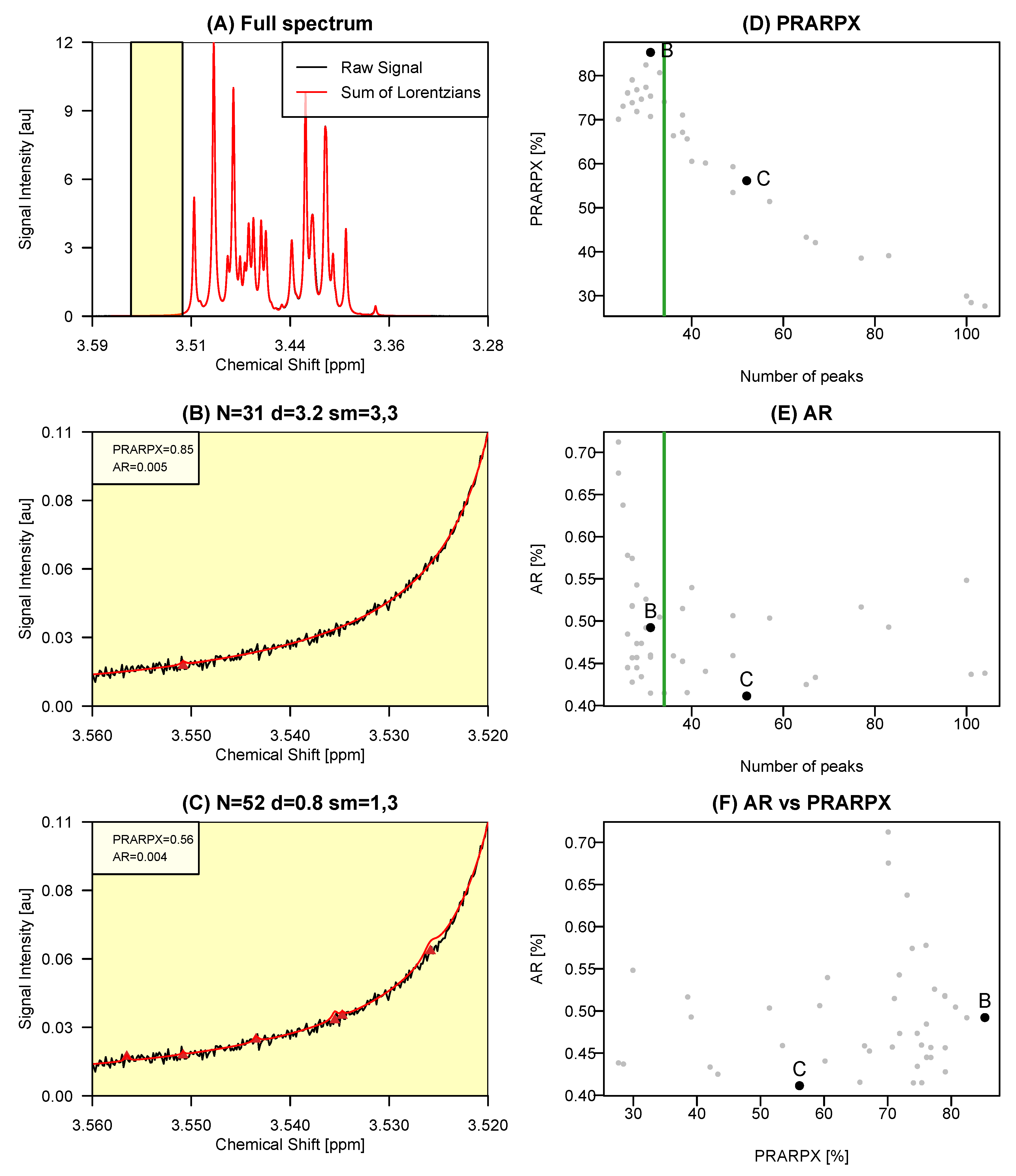
Figure A2.
Two intrinsic upper bounds on PRARPX, illustrated on the zero-shift reference spectrum of the Sim2 dataset. (A) The true-Lorentzian superposition (red) overlaid on the observed intensities (black), with the individual true Lorentzians shown as grey fills. PRX by construction (every true peak is present); the residual area equals the additive measurement noise and yields , so even this noiseless reconstruction cannot reach . (B) The deconvolution at the best-PRARPX cell of metabodeconplus’s default 60-cell grid. Peaks shadowed by larger neighbours produce no detectable curvature minimum and are therefore not recovered, pulling PRX below 1. Together the two panels visualise the noise-floor and shadowed-peak ceilings discussed in Section 3.1.
Figure A2.
Two intrinsic upper bounds on PRARPX, illustrated on the zero-shift reference spectrum of the Sim2 dataset. (A) The true-Lorentzian superposition (red) overlaid on the observed intensities (black), with the individual true Lorentzians shown as grey fills. PRX by construction (every true peak is present); the residual area equals the additive measurement noise and yields , so even this noiseless reconstruction cannot reach . (B) The deconvolution at the best-PRARPX cell of metabodeconplus’s default 60-cell grid. Peaks shadowed by larger neighbours produce no detectable curvature minimum and are therefore not recovered, pulling PRX below 1. Together the two panels visualise the noise-floor and shadowed-peak ceilings discussed in Section 3.1.
Appendix E. End-to-End AKI Benchmark: Supplementary Outputs
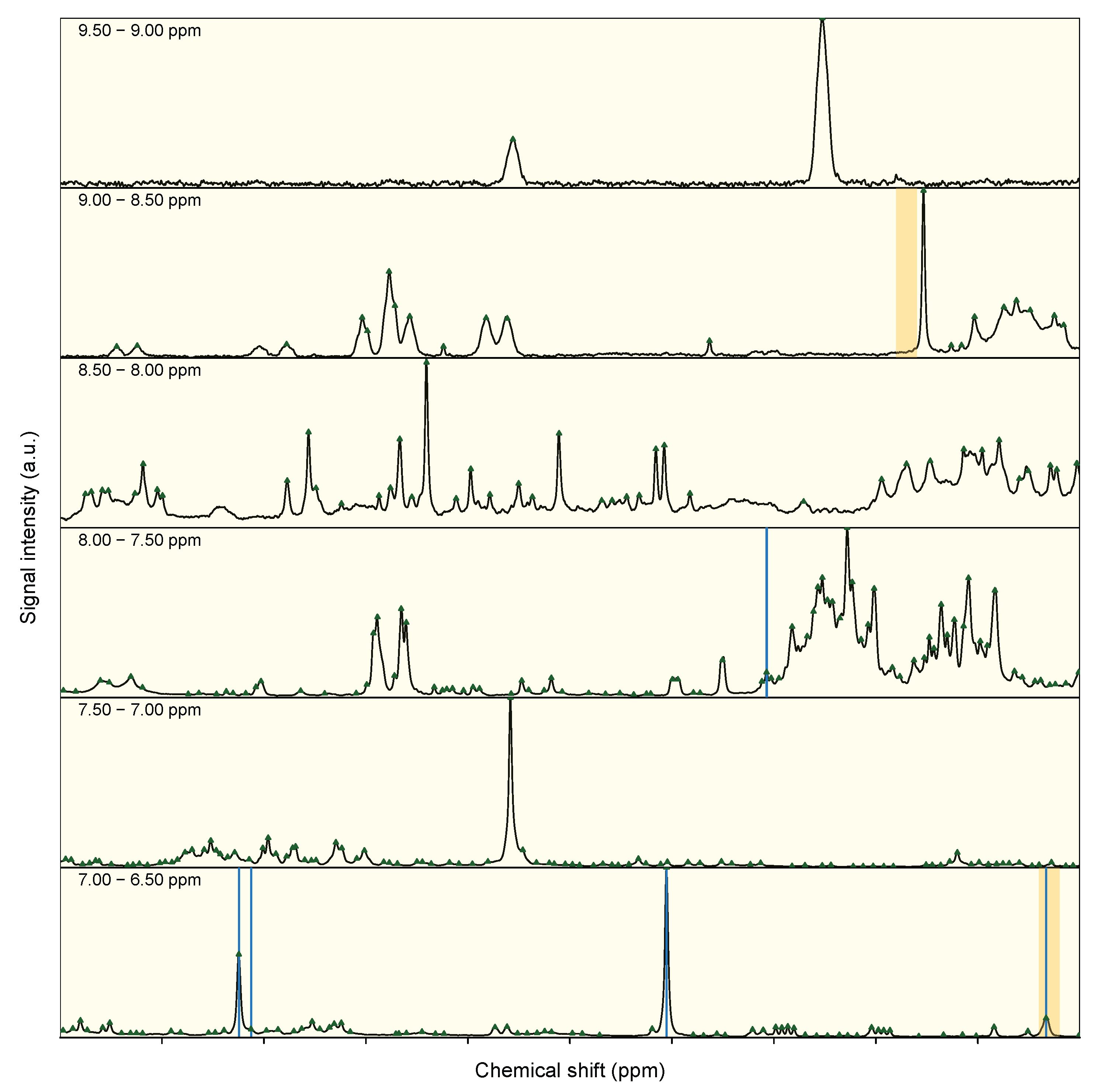
This appendix lists the discriminative features of the two classifiers underlying Figure 6. Both classifiers were trained on the full AKI dataset and their features were ranked by permutation importance, defined as the loss in classification accuracy that results from randomly shuffling a feature’s values across samples, averaged across the trees of the forest. report the twenty highest-ranked features of the binning baseline and of the metabodeconplus pipeline respectively, together with their chemical-shift positions and importance scores. Figure A3 is the aromatic-region counterpart to Figure 6: of the twenty highest-ranked features per model, two bins and five metabodeconplus peaks fall in the aromatic – ppm window, while the remainder occupy the aliphatic region shown in the main-text figure.
Table A2.
The twenty highest-ranked features of the binning-baseline random forest, trained on the full AKI dataset. Each row gives the chemical-shift interval covered by the bin and its permutation-importance score.
Table A2.
The twenty highest-ranked features of the binning-baseline random forest, trained on the full AKI dataset. Each row gives the chemical-shift interval covered by the bin and its permutation-importance score.
| Rank | Low (ppm) | High (ppm) | Importance |
|---|---|---|---|
| 1 | 3.500 | 3.510 | 0.0038 |
| 2 | 3.520 | 3.530 | 0.0025 |
| 3 | 1.390 | 1.400 | 0.0023 |
| 4 | 1.810 | 1.820 | 0.0018 |
| 5 | 1.620 | 1.630 | 0.0016 |
| 6 | 4.240 | 4.250 | 0.0015 |
| 7 | 3.550 | 3.560 | 0.0015 |
| 8 | 3.740 | 3.750 | 0.0014 |
| 9 | 4.360 | 4.370 | 0.0014 |
| 10 | 2.770 | 2.780 | 0.0013 |
| 11 | 1.410 | 1.420 | 0.0013 |
| 12 | 1.040 | 1.050 | 0.0013 |
| 13 | 3.580 | 3.590 | 0.0012 |
| 14 | 6.510 | 6.520 | 0.0011 |
| 15 | 1.180 | 1.190 | 0.0011 |
| 16 | 8.580 | 8.590 | 0.0011 |
| 17 | 1.260 | 1.270 | 0.0011 |
| 18 | 1.020 | 1.030 | 0.0011 |
| 19 | 3.000 | 3.010 | 0.0011 |
| 20 | 1.840 | 1.850 | 0.0010 |
Table A3.
The twenty highest-ranked features of the metabodeconplus pipeline (deconvolute → CluPA →snap_to_ref→ranger) at the grid cell selected by fit_mdm() on the full AKI dataset (, auto-tuned, ). Each row gives the chemical shift of the peak on the alignment reference and its permutation-importance score.
Table A3.
The twenty highest-ranked features of the metabodeconplus pipeline (deconvolute → CluPA →snap_to_ref→ranger) at the grid cell selected by fit_mdm() on the full AKI dataset (, auto-tuned, ). Each row gives the chemical shift of the peak on the alignment reference and its permutation-importance score.
| Rank | ppm | Importance |
|---|---|---|
| 1 | 1.9923 | 0.0031 |
| 2 | 1.6483 | 0.0031 |
| 3 | 1.6543 | 0.0029 |
| 4 | 6.9063 | 0.0026 |
| 5 | 6.9122 | 0.0025 |
| 6 | 6.5165 | 0.0024 |
| 7 | 2.8724 | 0.0024 |
| 8 | 2.8845 | 0.0023 |
| 9 | 1.2388 | 0.0023 |
| 10 | 1.0287 | 0.0019 |
| 11 | 3.8903 | 0.0018 |
| 12 | 1.1871 | 0.0017 |
| 13 | 3.4654 | 0.0016 |
| 14 | 1.3617 | 0.0016 |
| 15 | 1.2280 | 0.0014 |
| 16 | 1.6347 | 0.0013 |
| 17 | 6.7026 | 0.0012 |
| 18 | 7.6535 | 0.0012 |
| 19 | 3.8660 | 0.0012 |
| 20 | 1.1328 | 0.0012 |
Figure A3.
Aromatic-region counterpart to Figure 6, showing the – ppm window. Of the twenty highest-ranked features per model, two bins and five metabodeconplus peaks fall in this window; the rest lie in the aliphatic region shown in Figure 6. Layout and colour conventions match that figure: orange bands mark the bins selected by the binning model, blue vertical lines mark the peaks selected by the metabodeconplus model, and dark-green triangles mark every peak that metabodeconplus recovered from the reference spectrum.
Figure A3.
Aromatic-region counterpart to Figure 6, showing the – ppm window. Of the twenty highest-ranked features per model, two bins and five metabodeconplus peaks fall in this window; the rest lie in the aliphatic region shown in Figure 6. Layout and colour conventions match that figure: orange bands mark the bins selected by the binning model, blue vertical lines mark the peaks selected by the metabodeconplus model, and dark-green triangles mark every peak that metabodeconplus recovered from the reference spectrum.
References
- Gowda, G.N.; Zhu, W.; Raftery, D. NMR-based metabolomics: Where are we now and where are we going? Prog. Nucl. Magn. Reson. Spectrosc. 2025, 150–151, 101564. [Google Scholar] [CrossRef] [PubMed]
- Emwas, A.H.M. The Strengths and Weaknesses of NMR Spectroscopy and Mass Spectrometry with Particular Focus on Metabolomics Research. In Metabonomics: Methods and Protocols; Bjerrum, J.T., Ed.; Springer: New York, NY, 2015; pp. 161–193. [Google Scholar] [CrossRef] [PubMed]
- Levitt, M.H. Spin Dynamics: Basics of Nuclear Magnetic Resonance, 2 ed.; Wiley: Chichester, 2008. [Google Scholar]
- Keeler, J. Understanding NMR Spectroscopy, 2 ed.; Wiley: Chichester, 2010. [Google Scholar]
- Claridge, T.D.W. High-Resolution NMR Techniques in Organic Chemistry, third edition ed.; Elsevier: Amsterdam Boston Heidelberg London New York Oxford Paris, 2016. [Google Scholar]
- Beckonert, O.; Keun, H.C.; Ebbels, T.M.D.; Bundy, J.; Holmes, E.; Lindon, J.C.; Nicholson, J.K. Metabolic Profiling, Metabolomic and Metabonomic Procedures for NMR Spectroscopy of Urine, Plasma, Serum and Tissue Extracts. Nat. Protoc. 2007, 2, 2692–2703. [Google Scholar] [CrossRef] [PubMed]
- Hao, J.; Astle, W.; De Iorio, M.; Ebbels, T.M.D. BATMAN—an R Package for the Automated Quantification of Metabolites from Nuclear Magnetic Resonance Spectra Using a Bayesian Model. Bioinformatics 2012, 28, 2088–2090. [Google Scholar] [CrossRef] [PubMed]
- Canueto, D.; Gómez, J.; Salek, R.; Correig, X.; Cañellas, N. rDolphin: A GUI R Package for Proficient Automatic Profiling of 1D 1H-NMR Spectra of Study Datasets. Metabolomics 2018, 14. [Google Scholar] [CrossRef] [PubMed]
- Beirnaert, C.; Meysman, P.; Vu, T.N.; Hermans, N.; Apers, S.; Pieters, L.; Covaci, A.; Laukens, K. Speaq 2.0: A Complete Workflow for High-Throughput 1D NMR Spectra Processing and Quantification. PLoS Comput. Biol. 2018, 14, e1006018. [Google Scholar] [CrossRef] [PubMed]
- Lefort, G.; Liaubet, L.; Canlet, C.; Tardivel, P.; Père, M.C.; Quesnel, H.; Paris, A.; Iannuccelli, N.; Vialaneix, N.; Servien, R. ASICS: An R Package for a Whole Analysis Workflow of 1D 1H NMR Spectra. Bioinformatics 2019, 35, 4356–4363. [Google Scholar] [CrossRef] [PubMed]
- Khakimov, B.; Mobaraki, N.; Trimigno, A.; Aru, V.; Engelsen, S.B. Signature Mapping (SigMa): An Efficient Approach for Processing Complex Human Urine 1H NMR Metabolomics Data. Anal. Chim. Acta 2020, 1108, 142–151. [Google Scholar] [CrossRef] [PubMed]
- Häckl, M.; Tauber, P.; Schweda, F.; Zacharias, H.U.; Altenbuchinger, M.; Oefner, P.J.; Gronwald, W. An R-Package for the Deconvolution and Integration of 1D NMR Data: MetaboDecon1D. Metabolites 2021, 11, 452. [Google Scholar] [CrossRef] [PubMed]
- Hughes, T.S.; Wilson, H.D.; de Vera, I.M.S.; Kojetin, D.J. Deconvolution of Complex 1D NMR Spectra Using Objective Model Selection. PLoS ONE 2015, 10, e0134474. [Google Scholar] [CrossRef] [PubMed]
- Savorani, F.; Tomasi, G.; Engelsen, S. icoshift: A versatile tool for the rapid alignment of 1D NMR spectra. J. Magn. Reson. 2010, 202, 190–202. [Google Scholar] [CrossRef] [PubMed]
- Tomasi, G.; van den Berg, F.; Andersson, C. Correlation optimized warping and dynamic time warping as preprocessing methods for chromatographic data. J. Chemom. 2004, 18, 231–241. [Google Scholar] [CrossRef]
- Ravanbakhsh, S.; Liu, P.; Bjordahl, T.C.; Mandal, R.; Grant, J.R.; Wilson, M.; Eisner, R.; Sinelnikov, I.; Hu, X.; Luchinat, C.; et al. Accurate, Fully-Automated NMR Spectral Profiling for Metabolomics. PLoS ONE 2015, 10, e0124219. [Google Scholar] [CrossRef] [PubMed]
- Li, D.W.; Bruschweiler-Li, L.; Hansen, A.L.; Brüschweiler, R. DEEP Picker1D and Voigt Fitter1D: A Versatile Tool Set for the Automated Quantitative Spectral Deconvolution of Complex 1D-NMR Spectra. Magn. Reson. 2023, 4, 19–26. [Google Scholar] [CrossRef] [PubMed]
- Jacob, D.; Deborde, C.; Lefebvre, M.; Maucourt, M.; Moing, A. NMRProcFlow: A Graphical and Interactive Tool Dedicated to 1D Spectra Processing for NMR-based Metabolomics. Metabolomics 2017, 13, 36. [Google Scholar] [CrossRef] [PubMed]
- Schmid, N.; Bruderer, S.; Paruzzo, F.; Fischetti, G.; Toscano, G.; Graf, D.; Fey, M.; Henrici, A.; Ziebart, V.; Heitmann, B.; et al. Deconvolution of 1D NMR spectra: A deep learning-based approach. J. Magn. Reson. 2023, 347, 107357. [Google Scholar] [CrossRef] [PubMed]
- Vu, T.N.; Valkenborg, D.; Smets, K.; Verwaest, K.A.; Dommisse, R.; Lemiere, F.; Verschoren, A.; Goethals, B.; Laukens, K. An integrated workflow for robust alignment and simplified quantitative analysis of NMR spectrometry data. BMC Bioinform. 2011, 12, 405. [Google Scholar] [CrossRef] [PubMed]
- Titze, S.; Schmid, M.; Köttgen, A.; Busch, M.; Floege, J.; Wanner, C.; Kronenberg, F.; Eckardt, K.U. Disease burden and risk profile in referred patients with moderate chronic kidney disease: composition of the German Chronic Kidney Disease (GCKD) cohort. Nephrol. Dial. Transplant. 2015, 30, 441–451. [Google Scholar] [CrossRef] [PubMed]
- Zacharias, H.U.; Altenbuchinger, M.; Schultheiss, U.T.; Samol, C.; Kotsis, F.; Poguntke, I.; Sekula, P.; Jan, K.; Köttgen, A.; Spang, R.; et al. A Novel Metabolic Signature To Predict the Requirement of Dialysis or Renal Transplantation in Patients with Chronic Kidney Disease. J. Proteome Res. 2019, 18, 1796–1805. [Google Scholar] [CrossRef] [PubMed]
- Zacharias, H.U.; Schley, G.; Hochrein, J.; Klein, M.S.; Köberle, C.; Eckardt, K.U.; Willam, C.; Oefner, P.J.; Gronwald, W. Analysis of Human Urine Reveals Metabolic Changes Related to the Development of Acute Kidney Injury Following Cardiac Surgery. Metabolomics 2013, 9, 697–707. [Google Scholar] [CrossRef]
- Schley, G.; Köberle, C.; Manuilova, E.; Rutz, S.; Forster, C.; Weyand, M.; Formentini, I.; Kientsch-Engel, R.; Eckardt, K.U.; Willam, C. Comparison of plasma and urine biomarker performance in acute kidney injury. PLoS ONE 2015, 10, e0145042. [Google Scholar] [CrossRef] [PubMed]
- Koh, H.W.; Maddula, S.; Lambert, J.; Hergenröder, R.; Hildebrand, L. An approach to automated frequency-domain feature extraction in nuclear magnetic resonance spectroscopy. J. Magn. Reson. 2009, 201, 146–156. [Google Scholar] [CrossRef] [PubMed]
- Wright, M.N.; Ziegler, A. ranger: A Fast Implementation of Random Forests for High Dimensional Data in C++ and R. J. Stat. Softw. 2017, 77, 1–17. [Google Scholar] [CrossRef]
- Breiman, L. Statistical Modeling: The Two Cultures (with Comments and a Rejoinder by the Author). Stat. Sci. 2001, 16, 199–231. [Google Scholar] [CrossRef]
- Wright, M.N.; Wager, S.; Probst, P. ranger: A Fast Implementation of Random Forests, 2024. R package version 0.18.0. [CrossRef]
- Pang, Z.; Lu, Y.; Zhou, G.; Hui, F.; Xu, L.; Viau, C.; Spigelman, A.F.; MacDonald, P.E.; Wishart, D.S.; Li, S.; et al. MetaboAnalyst 6.0: towards a unified platform for metabolomics data processing, analysis and interpretation. Nucleic Acids Res. 2024, 52, W398–W406. [Google Scholar] [CrossRef] [PubMed]
Figure 1.
Visualization of the deconvolution algorithm for a small, simulated spectrum with four peaks. (a) Raw spectrum. (b) Smoothed spectrum after applying a moving average filter. (c) Peak detection on the smoothed spectrum: red triangles mark peak centers, blue squares mark peak borders. (d) Initial Lorentzian curve estimates before iterative refinement (nfit = 0). (e) Lorentzian curves after one iteration of refinement (nfit = 1). (f) Lorentzian curves after three iterations of refinement (nfit = 3). In (d)–(f), the black line shows the raw spectrum and the red line shows the superposition of the fitted Lorentzian curves.
Figure 1.
Visualization of the deconvolution algorithm for a small, simulated spectrum with four peaks. (a) Raw spectrum. (b) Smoothed spectrum after applying a moving average filter. (c) Peak detection on the smoothed spectrum: red triangles mark peak centers, blue squares mark peak borders. (d) Initial Lorentzian curve estimates before iterative refinement (nfit = 0). (e) Lorentzian curves after one iteration of refinement (nfit = 1). (f) Lorentzian curves after three iterations of refinement (nfit = 3). In (d)–(f), the black line shows the raw spectrum and the red line shows the superposition of the fitted Lorentzian curves.
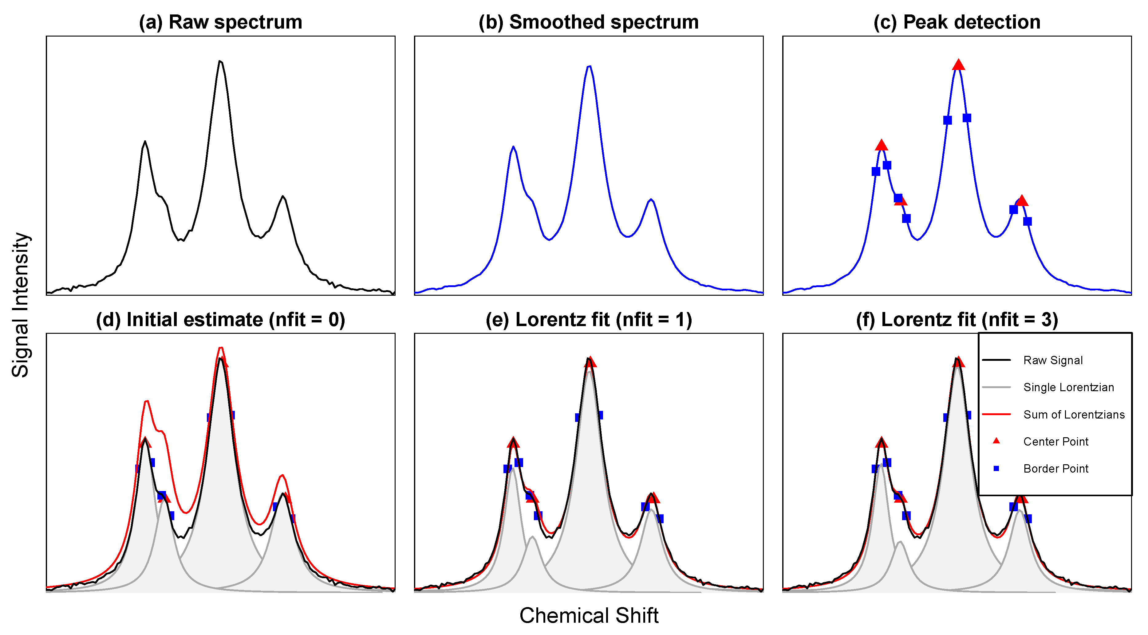
Figure 2.
Cumulative effect of the two-step alignment pipeline on the first six Sim2 spectra, zoomed to the window 3.415–3.450 ppm and run with and (the supervised joint optimum found on this dataset in Section 3.3). Top row (1A–1C): overlay of the reconstructed spectra after deconvolution (1A), after CluPA (1B), and after snap_to_ref() (1C); the reference spectrum is drawn in red, the others in dark grey. Middle row (2A–2C): the same six spectra rendered as intensity heatmaps (white-to-dark-blue colour scale); the reference row is outlined by a red rectangle. Bottom row (3A–3C): sparse peak-position heatmaps for the same stages – one vertical mark per fitted Lorentzian peak, located at its centre and shaded by its peak height ; cells with no peak are white. After snap_to_ref() (3C) every spectrum’s marks land exactly on the reference’s peak columns.
Figure 2.
Cumulative effect of the two-step alignment pipeline on the first six Sim2 spectra, zoomed to the window 3.415–3.450 ppm and run with and (the supervised joint optimum found on this dataset in Section 3.3). Top row (1A–1C): overlay of the reconstructed spectra after deconvolution (1A), after CluPA (1B), and after snap_to_ref() (1C); the reference spectrum is drawn in red, the others in dark grey. Middle row (2A–2C): the same six spectra rendered as intensity heatmaps (white-to-dark-blue colour scale); the reference row is outlined by a red rectangle. Bottom row (3A–3C): sparse peak-position heatmaps for the same stages – one vertical mark per fitted Lorentzian peak, located at its centre and shaded by its peak height ; cells with no peak are white. After snap_to_ref() (3C) every spectrum’s marks land exactly on the reference’s peak columns.
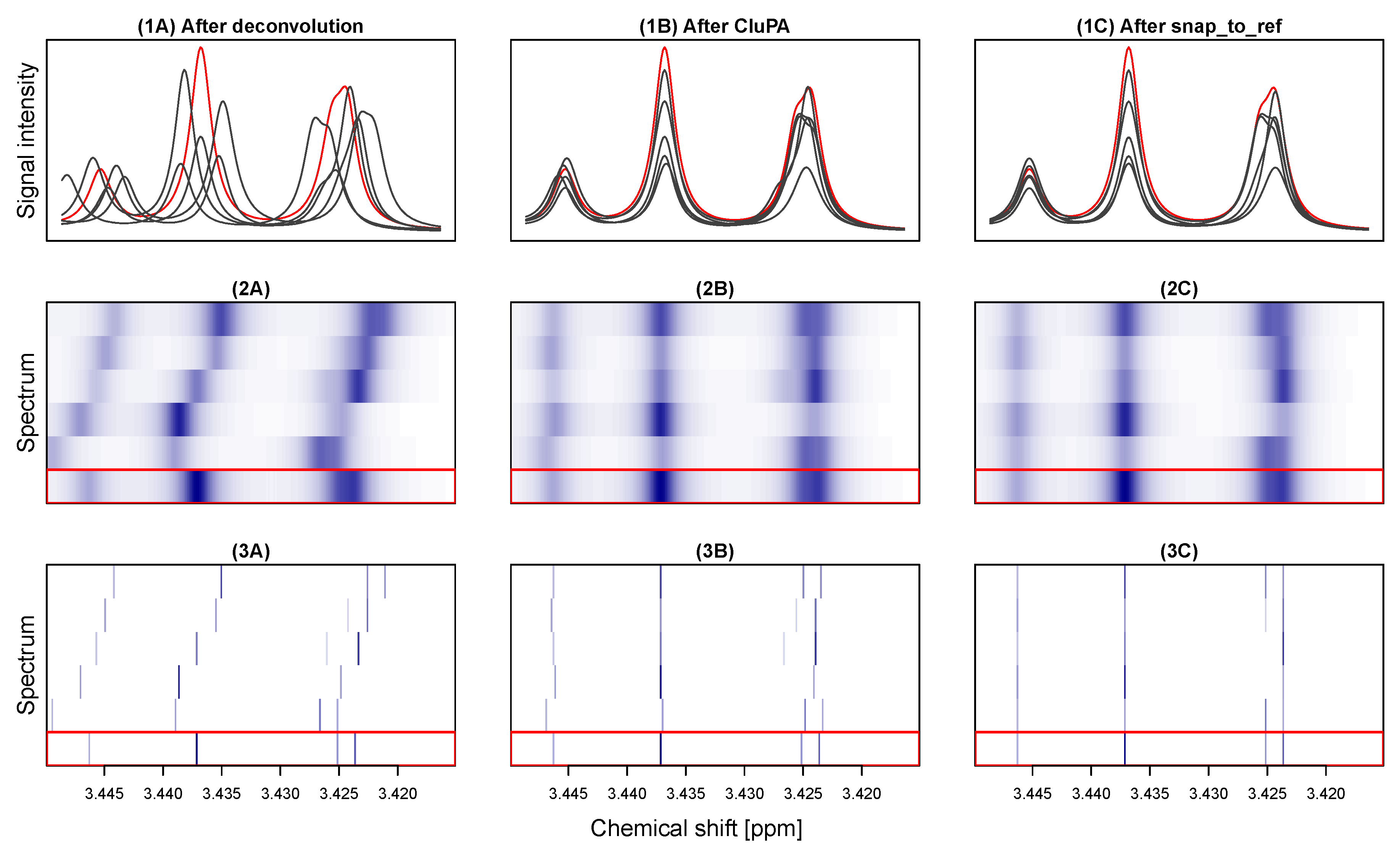
Figure 3.
Per-spectrum PRARPX on the 100 Sim2 spectra for each configuration in Table 3, sorted by ascending metabodeconplus optimal PRARPX (the best grid cell per spectrum) so the x-axis encodes intrinsic deconvolution difficulty, from hardest on the left to easiest on the right. Highlighted lines: MetaboDecon1D default (red), metabodeconplus default (blue), the best-mean grid-search configuration (green), and metabodeconplus optimal (dotted grey). The other grid-search configurations are drawn as faint grey lines.
Figure 3.
Per-spectrum PRARPX on the 100 Sim2 spectra for each configuration in Table 3, sorted by ascending metabodeconplus optimal PRARPX (the best grid cell per spectrum) so the x-axis encodes intrinsic deconvolution difficulty, from hardest on the left to easiest on the right. Highlighted lines: MetaboDecon1D default (red), metabodeconplus default (blue), the best-mean grid-search configuration (green), and metabodeconplus optimal (dotted grey). The other grid-search configurations are drawn as faint grey lines.
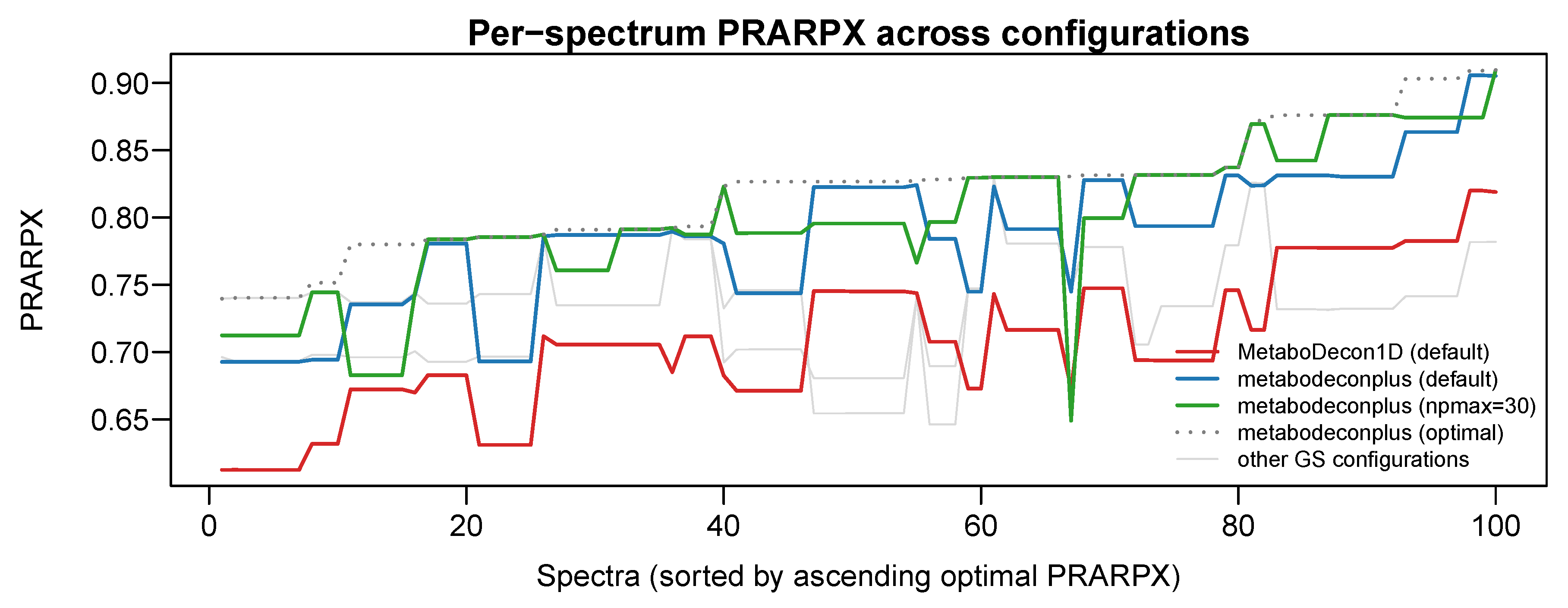
Figure 4.
Snap purity on all 100 Sim2 spectra over the grid. Each cell shows the fraction of (spectrum, true-peak-letter) pairs — in total — for which the deconvolution peak with the matching label was snapped onto its true reference column with no wrong-label peak in that column. The maxShift = 0 column is the no-CluPA baseline; the maxCombine = 0 row is CluPA only (no snap). Cells are shaded by a 20-step discrete YlOrRd color palette (one band per 5% interval; lighter = higher purity).
Figure 4.
Snap purity on all 100 Sim2 spectra over the grid. Each cell shows the fraction of (spectrum, true-peak-letter) pairs — in total — for which the deconvolution peak with the matching label was snapped onto its true reference column with no wrong-label peak in that column. The maxShift = 0 column is the no-CluPA baseline; the maxCombine = 0 row is CluPA only (no snap). Cells are shaded by a 20-step discrete YlOrRd color palette (one band per 5% interval; lighter = higher purity).
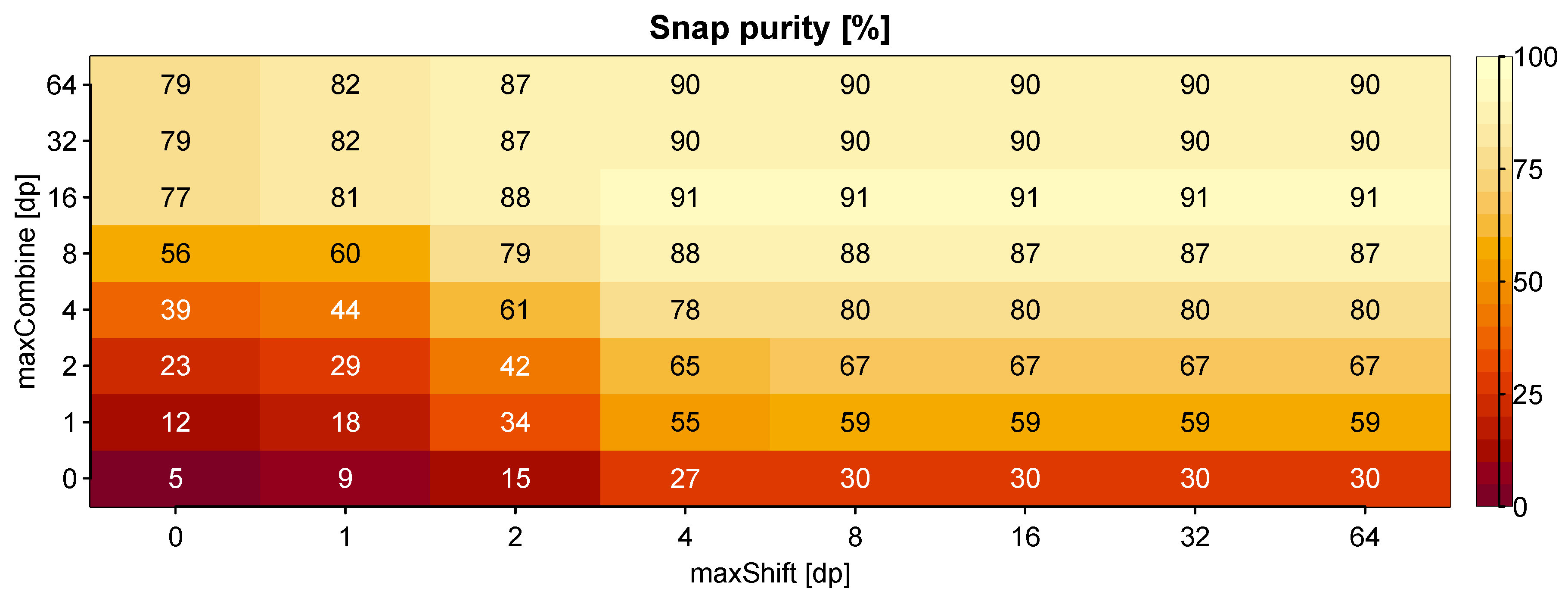
Figure 5.
Supervised parameter optimization on Sim2. (a) Out-of-bag accuracy for every row ×npmax column combination; rows are sorted by ascending and, within each , by ascending. The cell selected by fit_mdm() — the highest-OOB-accuracy combination, ties broken by AUC — is circled in red. (b) The same grid scored by OOB AUC, sharing both row order and the circled cell with (a) so that the chosen is the same row/column in both panels. Both panels use a viridis palette and cell-text annotations. (c) Heatmap of all ranger features obtained for the best parameter combination. Columns to the left of the center are features whose mean is higher in Group A (positive two-sample t-score); columns to the right are higher in Group B. Within each half, columns are sorted by ranger permutation importance ascending toward the center, so the most informative features are located nearest the outer edges. Tick labels of features within datapoints of a discriminative peak are coloured dark green and marked with an asterisk. Rows are training spectra, framed and labelled on the right by class (A, B). (d) Superposition of 5 group-A and 5 group-B training spectra after alignment and snapping, zoomed on the range of ranger features (plus ppm of padding), with one vertical line per feature shown in (c). Green lines mark features within datapoints of a discriminative peak (at most 3 by construction); grey lines mark the other ranger features. Line width scales with the ranger permutation importance of each feature, so that the most informative features stand out visually.
Figure 5.
Supervised parameter optimization on Sim2. (a) Out-of-bag accuracy for every row ×npmax column combination; rows are sorted by ascending and, within each , by ascending. The cell selected by fit_mdm() — the highest-OOB-accuracy combination, ties broken by AUC — is circled in red. (b) The same grid scored by OOB AUC, sharing both row order and the circled cell with (a) so that the chosen is the same row/column in both panels. Both panels use a viridis palette and cell-text annotations. (c) Heatmap of all ranger features obtained for the best parameter combination. Columns to the left of the center are features whose mean is higher in Group A (positive two-sample t-score); columns to the right are higher in Group B. Within each half, columns are sorted by ranger permutation importance ascending toward the center, so the most informative features are located nearest the outer edges. Tick labels of features within datapoints of a discriminative peak are coloured dark green and marked with an asterisk. Rows are training spectra, framed and labelled on the right by class (A, B). (d) Superposition of 5 group-A and 5 group-B training spectra after alignment and snapping, zoomed on the range of ranger features (plus ppm of padding), with one vertical line per feature shown in (c). Green lines mark features within datapoints of a discriminative peak (at most 3 by construction); grey lines mark the other ranger features. Line width scales with the ranger permutation importance of each feature, so that the most informative features stand out visually.
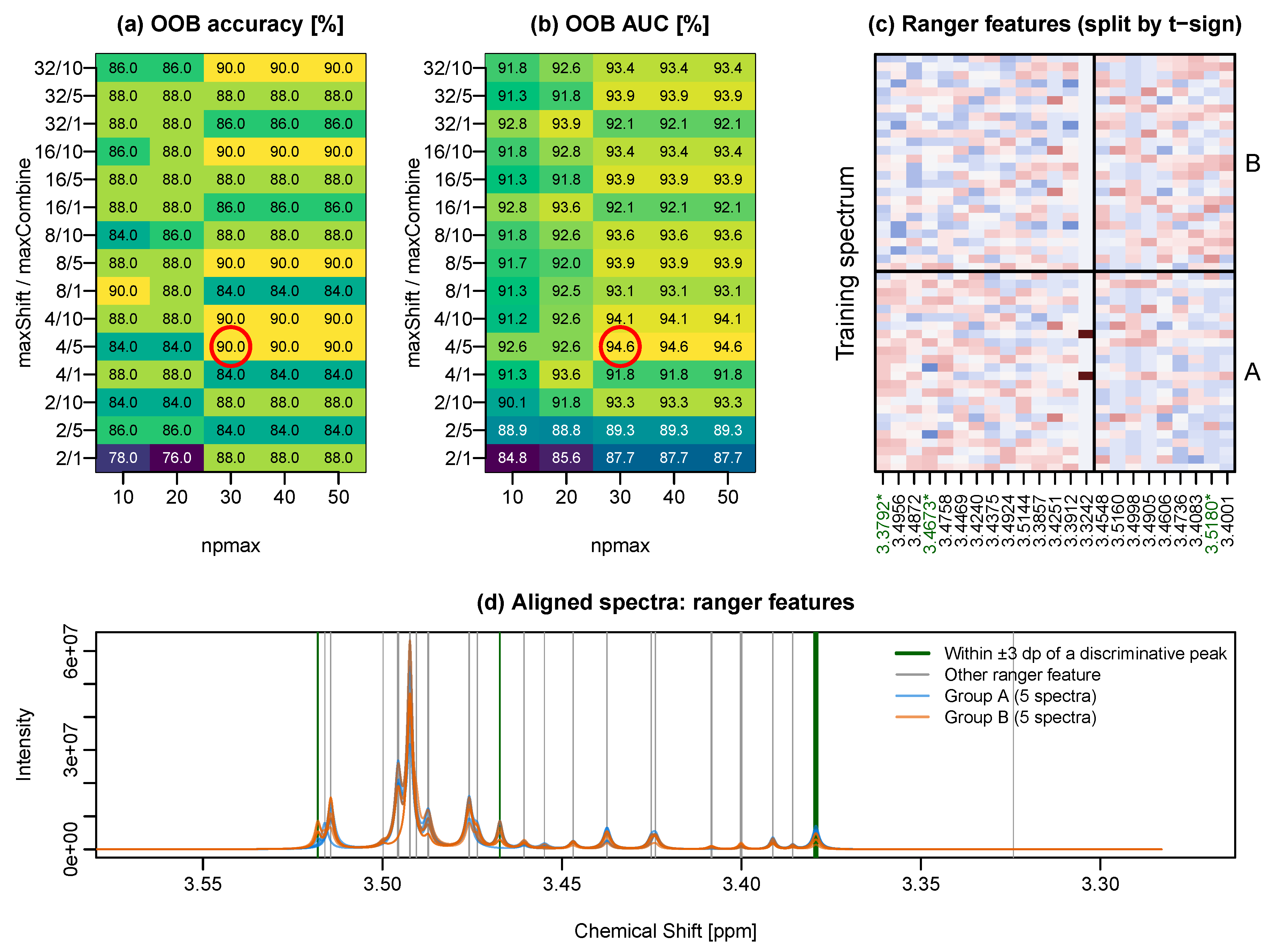
Figure 6.
The twenty most informative features of each of the two classification models — the equidistant-binning baseline and the metabodeconplus peak-based model — overlaid on the alignment reference spectrum across the aliphatic – ppm region. The figure is split into eight rows of ppm width each (top row – ppm, bottom row – ppm); within each row chemical shift increases from right to left as is customary for NMR. Orange bands mark the bins selected by the binning baseline; blue vertical lines mark the peaks selected by the metabodeconplus model. Dark-green triangles mark every peak that metabodeconplus recovered from the reference spectrum, drawn at the spectrum’s intensity at that position. Agreement between the two models is indicated by co-located orange bands and blue lines. Eighteen of the selected twenty bins and fifteen of the selected twenty peaks fall inside the aliphatic window shown here. The remaining features, located in the aromatic – ppm region, together with the full ranked lists, are given in Appendix E.
Figure 6.
The twenty most informative features of each of the two classification models — the equidistant-binning baseline and the metabodeconplus peak-based model — overlaid on the alignment reference spectrum across the aliphatic – ppm region. The figure is split into eight rows of ppm width each (top row – ppm, bottom row – ppm); within each row chemical shift increases from right to left as is customary for NMR. Orange bands mark the bins selected by the binning baseline; blue vertical lines mark the peaks selected by the metabodeconplus model. Dark-green triangles mark every peak that metabodeconplus recovered from the reference spectrum, drawn at the spectrum’s intensity at that position. Agreement between the two models is indicated by co-located orange bands and blue lines. Eighteen of the selected twenty bins and fifteen of the selected twenty peaks fall inside the aliphatic window shown here. The remaining features, located in the aromatic – ppm region, together with the full ranked lists, are given in Appendix E.
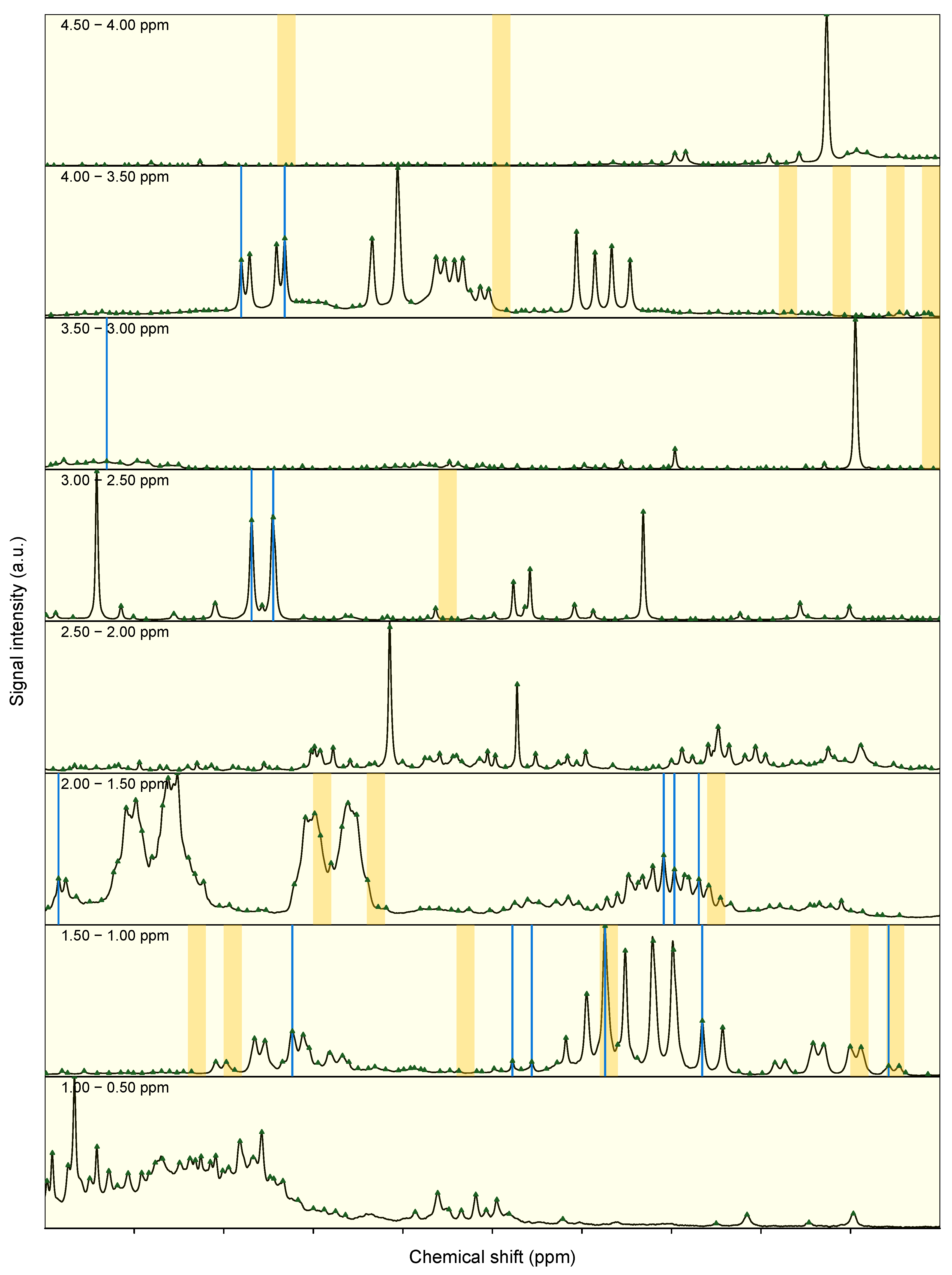
Figure 7.
Runtime performance. Panels (A)–(C) report single-core, single-spectrum wall-clock for the original MetaboDecon1D package, the R implementation of the new metabodeconplus package, and the Rust backend of metabodeconplus as activated from within the R environment, across spectrum sizes (– data points) and peak counts (–; one line per peak count, legend in panel A). Panel (D) reports the wall-clock for deconvoluting all 106 AKI urinary spectra at , separately for the pure-R and Rust backends, with a dashed reference curve marking ideal scaling anchored at the slower backend’s point; parallelisation is across spectra while per-spectrum deconvolution remains single-threaded. All timings averaged over 5 repetitions per cell (panels A–C) or per value (panel D); measurements taken on a Xeon Gold 6348 workstation.
Figure 7.
Runtime performance. Panels (A)–(C) report single-core, single-spectrum wall-clock for the original MetaboDecon1D package, the R implementation of the new metabodeconplus package, and the Rust backend of metabodeconplus as activated from within the R environment, across spectrum sizes (– data points) and peak counts (–; one line per peak count, legend in panel A). Panel (D) reports the wall-clock for deconvoluting all 106 AKI urinary spectra at , separately for the pure-R and Rust backends, with a dashed reference curve marking ideal scaling anchored at the slower backend’s point; parallelisation is across spectra while per-spectrum deconvolution remains single-threaded. All timings averaged over 5 repetitions per cell (panels A–C) or per value (panel D); measurements taken on a Xeon Gold 6348 workstation.
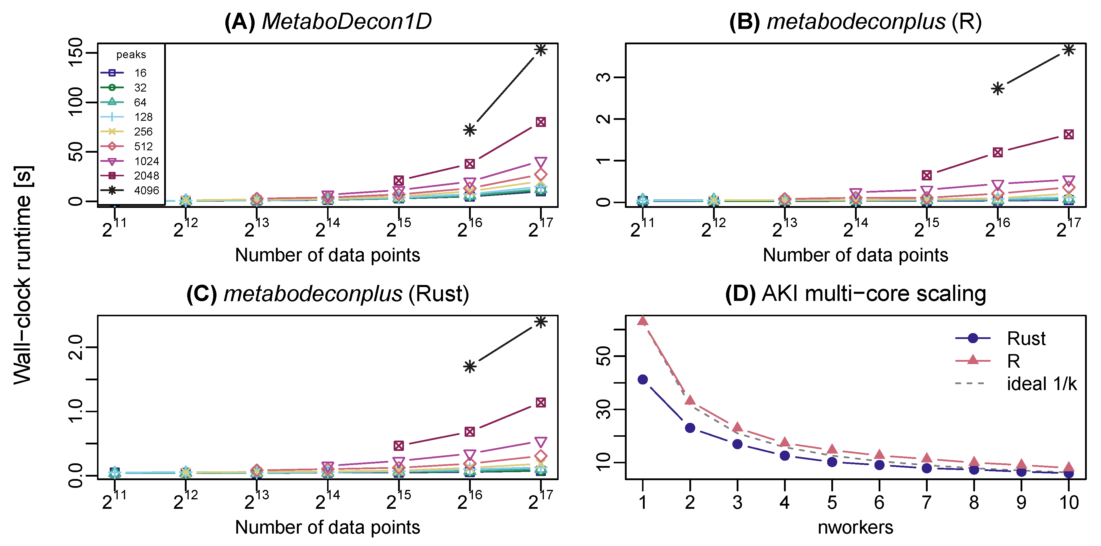
Table 1.
Summary of tasks performed by various published approaches. aIndicated are only approaches that perform a dedicated signal deconvolution of overlapping signals. bTools that allow an absolute quantification of metabolites. cApproaches performing a dedicated signal alignment, allowing for non-linear signal corrections, across a set of measured spectra. dAdditional tools to perform a statistical analysis of obtained data. eCommercial approaches.
Table 1.
Summary of tasks performed by various published approaches. aIndicated are only approaches that perform a dedicated signal deconvolution of overlapping signals. bTools that allow an absolute quantification of metabolites. cApproaches performing a dedicated signal alignment, allowing for non-linear signal corrections, across a set of measured spectra. dAdditional tools to perform a statistical analysis of obtained data. eCommercial approaches.
| Name | Deconvolutiona | Quantificationb | Alignmentc | Statisticsd |
|---|---|---|---|---|
| ACD/NMRe | ✓ | ✓ | – | ✓ |
| AMIXe | ✓ | ✓ | – | ✓ |
| Asics | ✓ | ✓ | – | ✓ |
| Batman | ✓ | ✓ | – | – |
| Bayesil | ✓ | ✓ | – | – |
| Chenomxe | ✓ | ✓ | – | – |
| COW | – | – | ✓ | – |
| Decon1d | ✓ | – | – | – |
| Deep Picker1D | ✓ | – | – | – |
| Icoshift | – | – | ✓ | – |
| metabodeconplus | ✓ | ✓ | ✓ | ✓ |
| MetaboDecon1D | ✓ | – | – | – |
| Mldecon | ✓ | – | – | ✓ |
| MNova NMRe | ✓ | ✓ | – | ✓ |
| NMRProcFlow | – | – | ✓ | ✓ |
| rDolphin | ✓ | ✓ | – | – |
| SigMa | ✓ | ✓ | ✓ | – |
| Speaq 2.0 | – |
Table 2.
Summary of sample types, number of samples, and measurement techniques used. The Blood dataset seeds the reference peak parameters of the simulated Sim2 dataset (Section 3.1); the Urine dataset is used to select the default npmax for the AKI benchmark (Section 3.4).
Table 2.
Summary of sample types, number of samples, and measurement techniques used. The Blood dataset seeds the reference peak parameters of the simulated Sim2 dataset (Section 3.1); the Urine dataset is used to select the default npmax for the AKI benchmark (Section 3.4).
| Name | Sample Type | Number of Samples | Exp. Technique |
|---|---|---|---|
| Sim2 | Simulated | 100 | 1D Sim |
| Blood | Human Blood Plasma | 16 | 1D CPMG |
| Urine | Human Urine | 2 | 1D NOESY |
| AKI | Human Urine | 106 | 1D NOESY |
Table 3.
PRARPX summary on the Sim2 dataset across all spectra: mean, standard deviation, minimum, and maximum for each configuration. Bold marks the best achievable (mean, sd) pair (highest mean, ties broken by smallest sd); the metabodeconplus optimal row is excluded from this comparison.
Table 3.
PRARPX summary on the Sim2 dataset across all spectra: mean, standard deviation, minimum, and maximum for each configuration. Bold marks the best achievable (mean, sd) pair (highest mean, ties broken by smallest sd); the metabodeconplus optimal row is excluded from this comparison.
| Configuration | mean | sd | min | max |
|---|---|---|---|---|
| MetaboDecon1D (default) | 0.708 | 0.052 | 0.612 | 0.820 |
| metabodeconplus (default) | 0.785 | 0.053 | 0.693 | 0.906 |
| metabodeconplus (npmax=10) | 0.727 | 0.040 | 0.646 | 0.829 |
| metabodeconplus (npmax=20) | 0.740 | 0.036 | 0.654 | 0.829 |
| metabodeconplus (npmax=30) | 0.798 | 0.054 | 0.649 | 0.910 |
| metabodeconplus (npmax=40) | 0.798 | 0.054 | 0.649 | 0.910 |
| metabodeconplus (npmax=50) | 0.798 | 0.054 | 0.649 | 0.910 |
| metabodeconplus (optimal) | 0.820 | 0.044 | 0.740 | 0.910 |
Disclaimer/Publisher’s Note: The statements, opinions and data contained in all publications are solely those of the individual author(s) and contributor(s) and not of MDPI and/or the editor(s). MDPI and/or the editor(s) disclaim responsibility for any injury to people or property resulting from any ideas, methods, instructions or products referred to in the content. |
© 2026 by the authors. Licensee MDPI, Basel, Switzerland. This article is an open access article distributed under the terms and conditions of the Creative Commons Attribution (CC BY) license (http://creativecommons.org/licenses/by/4.0/).
Copyright: This open access article is published under a Creative Commons CC BY 4.0 license, which permit the free download, distribution, and reuse, provided that the author and preprint are cited in any reuse.


