

Submitted:
16 July 2026
Posted:
17 July 2026
You are already at the latest version
Abstract
We ask how fast high-fidelity gear rattle can be simulated—and where, once chaos sets in, simulating trajectories stops being useful and must give way to computing structure. By high-fidelity we mean a nonsmooth model that retains the three-state backlash, a time-varying mesh stiffness, tooth friction, and a flexible modal reduction of the gear bodies. Exploiting the piecewise-linear structure, we propagate each backlash state with a segment-exact exponential step and fuse many mesh cycles into a single spectral map: the constant-contact fusion advances one mesh cycle in a single matrix–vector product (∼61 ns) and jumps 106 cycles in 634 ns, while the sparse-regime event-driven path reaches 16× real time with a brute-force cross-check at 7 × 10⁻¹⁵. We then show that singletrajectory depth and ensemble breadth strike the same memory-bandwidth wall, so a 56-core rattle atlas returns only 16.6× speedup (∼30% efficiency). Finally, with a largest Lyapunov exponent of ∼0.55 per rattle cycle, exponential compute buys only a linear gain in predictable horizon: beyond this Lyapunov wall the real-time target must shift from trajectories to invariant structure (Floquet skeletons, basin and attractor statistics). We report honest negative results, including a flexible model that admits no stable period-1 orbit (0/80 operating points).
Keywords:
gear rattle
; nonsmooth dynamics
; piecewise-linear systems
; exact propagation
; real-time simulation
; backlash
; Lyapunov exponent
; Floquet analysis
; memory-bandwidth wall
1. Introduction
Gear rattle is the audible signature of an unloaded or lightly loaded gear pair whose teeth repeatedly cross the backlash gap and impact on drive and coast flanks. It is a canonical piecewise-smooth mechanical system: between impacts the mesh contributes no restoring force, while inside contact the teeth engage through a time-varying, load-dependent mesh stiffness. The resulting equations of motion switch between distinct smooth vector fields at state-dependent events, and the closed-loop response is strongly nonlinear, exhibiting multi-flank impacts, subharmonics, and chaos. This behaviour has been documented and modelled for more than three decades: the periodically forced piecewise-linear oscillator provides the reduced archetype [1]; impact-map and gearbox studies traced the origin of chaotic rattle [2]; the gear-pair model with periodic stiffness and backlash established the reference nonlinear dynamics [3]; motor-driven configurations added the actuation loop [4]; and both refined models [5] and combined experimental–theoretical work [6] have continued to sharpen the picture of backlash-driven vibro-impact. The physics is, in this sense, well understood. What is not settled is a pair of engineering questions that the title of this paper poses directly.
How fast can high-fidelity gear rattle be simulated? By high-fidelity we mean a model that retains the features practitioners actually care about — the three-state backlash (drive contact, free flight, coast contact), a time-varying mesh stiffness excitation, tooth friction, and a flexible reduction of the gear bodies rather than a lumped two-mass caricature. Simulating such a model faster than real time is a prerequisite for hardware-in-the-loop powertrain testing [7] and for the real-time multibody workflows now being catalogued systematically [8]. The naive route — a stiff adaptive integrator chattering across every flank crossing — is far too slow, and it is also needlessly inaccurate, because the exact solution of each smooth segment is available in closed form.
Where does trajectory simulation give way to structure? Speed is not without consequence. Rattle is chaotic, so a computed trajectory is trustworthy only for a finite predictability horizon set by the largest Lyapunov exponent [9,10]. Past that horizon a faster point-trajectory buys essentially nothing: the meaningful object of computation ceases to be the trajectory and becomes the invariant structure — periodic-orbit skeletons, their stability, and the statistics of the attractor. One of our aims is to locate this crossover quantitatively and to show that beyond it real-time effort is better spent on structure than on integrating one more decorrelating path.
We are deliberately explicit about what is and is not new here. The enabling tools are all prior art. Segment-exact propagation by exponential integrators is a mature body of work [11,12], including breakpoint-stepping variants for switched systems [13]; the general theory and numerics of nonsmooth integration are likewise established [14,15]. Linearising the flow across an event uses the saltation matrix [15,16], and the performance ceiling of any such kernel is read off the Roofline model [17]. The predictability argument rests on finite-time Lyapunov analysis and its recent extensions [9,10]. We introduce none of these. Our contribution is instead to assemble them into a coherent, measured account of a single hard problem, and specifically:
- (i)
- high-fidelity super-real-time integration of a nonsmooth gear-rattle model, achieved by propagating each backlash state with a segment-exact exponential step and fusing many mesh cycles into a single spectral map — the constant-contact fusion advances one mesh cycle in a single matrix–vector product (∼61 ns) and jumps cycles in 634 ns, while the sparse-regime event-driven path reaches real time with a brute-force cross-check at ;
- (ii)
- the observation that single-trajectory depth and ensemble breadth hit the same wall — both saturate against memory bandwidth rather than arithmetic, so a 56-core rattle atlas returns speedup (about efficiency, not ), the same bandwidth ceiling that also caps the deepest single-path fusion;
- (iii)
- the identification of a Lyapunov wall — with a largest exponent of ∼0.55 per rattle cycle, exponential compute buys only a linear gain in predictable horizon, so beyond the wall real time must shift from trajectories to structure (Floquet skeletons, basin and attractor statistics);
- (iv)
- honest negative results — where fusion does not pay, where added modal fidelity is not worth its cost, and where the flexible model admits no stable period-1 orbit at all ( operating points), so the accessible range is entirely chaotic.
These findings are summarised by the flagship layered-ceiling map of Figure 1, which collects the achievable real-time factor as a function of model fidelity and integration strategy and marks the bandwidth and Lyapunov walls that bound the whole design space. As a headline calibration of the two questions above: at fixed accuracy the exact-fused kernel reaches an error of at ms/solve, against a high-order adaptive reference (Vern7 at tolerance ) that returns error at ms — roughly times faster and times more accurate, because exactness on each smooth segment removes both the cost and the local error of adaptive stepping.
The remainder of the paper is organised as follows. Section 2 states the nonsmooth gear-rattle model and its flexible reduction. Section 3 develops the segment-exact and spectral-fusion kernels and the event-driven path (Algorithms A1–A3), reports the tier ladder (Table 1) and the event-path progression (Table 2), and closes with the Roofline analysis of the shared depth/breadth memory wall (Figure 4). Section 4 turns to structure past the Lyapunov wall — the predictability crossover (Figure 7, Figure 8), the chaos atlas and bifurcation sweep (Figure 9, Figure 10), the Floquet skeleton (Figure 11), the NVH and phase-space signatures (Figure 12, Figure 13), and the degree-of-freedom convergence (Figure 14). Section 5 collects the negative results (Table 5), Section 6 the related work, and Section 7 concludes. Derivations, the optimisation history, validation, and the computing environment are deferred to the appendices.
2. A High-Fidelity Nonsmooth Gear Model
We study a spur gear pair driven near a mesh-order resonance, modelled at a fidelity that resolves the deformation-compatible tooth compliance, the flexibility of the connecting shafts, tooth friction, and the backlash-induced loss and re-establishment of contact. Figure 2 lays out the five concrete test cases used throughout the paper side by side — from a 2-DOF torsional pair to the flexible-shaft, three-state-backlash configuration — together with the shared mesh-stiffness engine that feeds all of them; the tiers differ only in which degrees of freedom are released. The full derivation, parameter set, and the exact segment propagator are deferred to A; here we state only the structure that the rest of the paper exploits, namely that the model is piecewise-linear time-invariant between well-defined switching events.
Deformation-compatible time-varying mesh stiffness.
The mesh compliance is obtained by an improved potential-energy method [18,19], in which each engaged tooth pair contributes bending, shear, axial and Hertzian-contact energy, summed over the instantaneous contact lines to give the time-varying mesh stiffness (TVMS) as a function of mesh phase . Profile modification and misalignment are admitted through the deformation-compatibility condition: under a misalignment measured by a single effective angular deviation , part of the flank may unload, so that the tangent mesh stiffness and the load centroid depend jointly on and the transmitted torque T. Both the loaded static transmission error and this coupling between backlash, transmission error and TVMS follow the pathway documented in [20]. In the dynamic model , and the static transmission error enter as prescribed, tabulated functions of mesh phase; within a mesh sub-interval they are treated as constant, which is the first source of piecewise structure. Two verified properties of this excitation pathway matter later. First, the misalignment loop is self-consistent: closing the slow feedback (dynamic response stiffness table) at mrad and 50 N m converges to a mean mesh stiffness below nominal, matching the partial-contact drop that the static table predicts independently. Second, parametric stiffness variation alone cannot produce rattle: under pure excitation the separation margin scales with the response itself and the teeth never leave contact — it is the displacement excitation near a mesh resonance that opens the gap, so the rattle studied here is STE-driven, not parametrically driven.
Flexible-shaft modal degrees of freedom.
The pinion and gear are carried on flexible shafts, reduced by modal truncation to N retained shaft/disc modes per member. The generalized coordinate is , collecting the modal amplitudes together with the mesh coordinate; the dynamic-transmission-error contribution of every mode enters the mesh only through a rank-one coupling vector , so that misalignment (through ) rotates a single coupling direction rather than restructuring the operator. Truncated modes are handled by residual (mode-acceleration / attachment) augmentation to restore the quasi-static flexibility they carry [21,22], consistent with finite-element geared-rotor practice [23] and component-mode reduction [24]. The retained system has dimension .
Tooth friction.
Sliding friction on the flanks is included as a Coulomb law , where is the mesh load, the friction coefficient and the sign/lever function that reverses at the pitch point. Because is fixed on each sub-interval, the friction generalized force is affine in the state there; it renders the segment operator non-symmetric (non-conservative) but does not break its linearity.
Three contact states and the backlash half-gap.
Backlash of half-gap b makes the mesh restoring law a three-state piecewise-linear map [1,3,4]: a free state (, no tooth load), a drive-side contact state () and a back-side contact state (). The switching surfaces separate three affine vector fields, giving a nonsmooth (Filippov-type) mechanical system [14,15]. Only in the contact states do the mesh stiffness and damping act; in the free state the mesh transmits no load and the two members interact only through the shafts. Crossing a switching surface is an impact-like event that must be located, not stepped over.
Augmented piecewise-linear state.
Collecting the modal and mesh coordinates with an appended constant “carry” coordinate that transports the external torque and the static-transmission-error excitation, we obtain an augmented state whose evolution on each segment (a fixed contact state and a fixed mesh sub-interval) is linear time-invariant,
with the affine excitation absorbed into the carry coordinate so that is a genuine matrix and within the segment. A trajectory is thus a concatenation of exact LTI flights joined at two kinds of breakpoints: mesh sub-interval boundaries, where changes because change; and contact-state switches at , where both the active vector field and (through the damping discontinuity) the transition map change. The exact per-segment propagator , the switching-surface event localization, and the state-transition (saltation) correction at are given in Appendix A and summarized as Algorithm 1; the whole of the present paper is an investigation of how far this exact piecewise-linear structure can be pushed before physics, rather than arithmetic, sets the limit.
3. Exact Propagation and the Real-Time Frontier
The model of Section 2 is piecewise-affine: within each contact state the dynamics are linear, and the only nonlinearity is the switching between states. This structure is not new, and neither is the observation that a linear segment can be advanced by its matrix exponential rather than by a general-purpose stepper; exponential integrators and their piecewise-linear specialisations are mature technology [11,12,13], and closed-form treatments of clearance and piecewise-linear oscillators have been given semi-analytically [25,26]. Our contribution here is not a new integrator but a measurement: applied to a high-fidelity nonsmooth gear-rattle model and pushed to its limits, exact propagation runs faster than real time, and we can say precisely how fast, where the speed comes from, and where it stops. Throughout, “×” denotes the wall-clock speed-up over real time, and all timings are single-core unless stated otherwise.
3.1. Constant-contact Regime: a Mesh Cycle in One Matvec
When the tooth pair stays in contact, the mesh cycle is a single affine segment and its time-T flow is one constant propagator acting on the state, precomputed once and reused for every cycle. Advancing a whole mesh period then costs a single matrix–vector product, ns for the low-dimensional lumped model. Because contact is smooth over many cycles, the composition can be assembled by repeated squaring: dyadic power-jumping advances mesh cycles in 634 ns, a speed-up over cycle-by-cycle marching, at the cost of storing dyadic factors. The Tier ladder of Table 1 reports the small-step (non-fused) real-time factor as the lumped dimension grows: at 2-DOF, at 6-DOF, at 12-DOF, at 20-DOF, and at the 40-mode flexible case (state dimension 81), the first point that falls below real time. The fused propagator recovers all of this and more: on the Tier-5 flexible configuration with Coulomb friction (), constant-contact simulation moves from small-step to with -segment propagation and to with fusion, while segment- and fused-propagation agree to and the transmission-error RMS differs by only ( vs. m) against the reference model. Constant contact is therefore essentially free; the cost of the problem lives entirely in the switching.
3.2. Nonsmooth Regime: Closed-Form Event Location and Segment Fusion
Under rattle the trajectory crosses backlash boundaries, and the wall-clock cost is set by how expensively each crossing is located. Event-driven integration of nonsmooth systems is standard [14,27], as is the use of switch detection to place discontinuities exactly [28], and the impact-map view of gearbox chaos dates to Hongler and Streit [2]. What matters for speed is that inside an affine segment the guard function is a known combination of exponentials, so the next crossing is the smallest root of a scalar transcendental equation rather than the output of a bisection over full state steps. Table 2 traces the resulting optimisation path for strong rattle at (tooth-passage time s). A naive segmented propagator (V1) needs 371 matvec per cycle (); reusing propagators (V2) drops this to 193 (); and closed-form spectral event location (V3) reaches 74 matvec plus 124 cheap scalar guard evaluations per cycle, still but now dominated by the physics of the impacts rather than by root-finding overhead. In the sparse-rattle regime () the same V3 path takes matvec and s per cycle for a real-time factor, and cross-checks against a brute-force reference to . The segment-fusion procedure that composes consecutive same-state segments is given as Algorithm 2 in Appendix C, with the spectral event solver in Algorithm 1. Exact event location is thus what keeps the nonsmooth regime above real time, but its per-cycle cost is bounded below by the event rate, which is a property of the trajectory, not of the algorithm.
3.3. High-Dimensional Flexible Configuration and the Memory-Bandwidth Wall
The most demanding configuration couples flexible modal DOFs, a three-state backlash, and Coulomb friction, with state dimension for N retained modes. Here two facts dominate. First, the constant-contact propagator is far better conditioned than the free-flight one— in contact versus free—and the spectral eigenbasis reconstructs the state to , so exactness is not the obstacle. The spectral event table costs 18 MB, against 190 MB if the same coverage were stored as dyadic power factors, and the spectral solution tracks brute force at the expected first-order rate ( at the working step) with an event rate of – per cycle. Second, and decisively, the propagator matvec is memory-bound. Measured matvec cost grows as s at dimension 31, s at 41, and s at 81: the jump is the L1 crossing, since an double-precision matrix is 52 KB and no longer fits the 32 KB L1 cache, placing the knee near 22 DOF. Model-order reduction is therefore not accuracy hygiene but a throughput device—keeping the working matrix resident in L1—and the relevant reduction machinery (mode acceleration, modal truncation augmentation, residual-attachment and dual Craig–Bampton synthesis, and data-driven reduction for piecewise-linear structures) is established prior art [21,22,24,29]. The optimisation chain of Figure 3 and Table 3 shows the payoff near resonance: the raw model (dimension 81) runs at (s, 120 matvec per solve), below real time; truncating to (dimension 41) with a simple projection reaches ; adding modal truncation augmentation (Algorithm 3) holds accuracy at ; and combining MTA with segment fusion reaches (s, 52 matvec)—the same physics now above real time. The MTA residual flexibility amounts to a static softening (), and the displacement-RMS is preserved to better than across the chain ( mm full-, simple-, MTA-). Internal consistency is exact—fusion versus spectral agree to and spectral versus brute to . Table 4 collects the full-configuration figures. The fidelity–cost trade is lopsided: fidelity is cheap until the working set leaves cache (Figure 5a), after which every added mode is paid for in bandwidth.
3.4. The Unified Wall
The L1 crossing of Section 3.3 is one face of a single limit. Making one trajectory deeper (more modes, longer horizons) and running more trajectories at once (an ensemble sweep) are throttled by the same resource, and the Roofline model [17] together with memory-bound performance prediction for stencil-type kernels [30] names it: at the propagator’s low arithmetic intensity the kernel sits under the bandwidth roof, not the compute roof. Figure 4 shows both faces meeting the same ceiling. On the ensemble side we compute a rattle atlas of 80 operating points (8 loads × 10 speeds) with 8 contact-state tables preloaded: the 56-core parallel run takes s against s serial, a speed-up—not the that core count would suggest, but roughly parallel efficiency, because the shared propagator and table traffic saturate memory bandwidth long before the cores saturate. Depth and breadth are throttled by one wall, and neither exponential-in-cost strategy escapes it.
Because hardware performance counters are unavailable under WSL2 (the Microsoft kernel does not virtualize the PMU), we characterize the memory system directly, by microbenchmark, using the production matvec kernel itself (Figure 5). Three measurements pin the wall down. First, a memory mountain: applying the solver’s own column-major saxpy kernel to a rotating set of operators — emulating how a mesh cycle walks through its spectral table — shows a cost that is flat while the rotating working set stays inside the 35 MB socket L3, then jumps (dim 81: s per matvec) once it spills to DRAM. At matched residency the per-operator cost scales essentially arithmetically with ; the hard cliff belongs to the table, not to the single operator. Second, aggregate streaming bandwidth saturates at ≈32 GB/s with only 14 of the 56 hardware threads — barely one core’s GB/s — and then decreases to 22 GB/s at 56 threads under NUMA and oversubscription pressure. Third, thread scaling of the full spectral solver on a shared table saturates at 25– on 56 threads, and the harder 8-table atlas workload at the already quoted. The traffic arithmetic closes the argument: a raw-N40 mesh cycle performs 120 matvecs against 52 KB operators, about MB of table traffic per cycle, so the cycle is a bandwidth workload rather than a flop workload. Appendix F maps every working set of the solver onto the machine’s cache hierarchy explicitly (Figure A2); read this way, MTA reduction, segment fusion, and the spectral-table layout are all the same move — relocating this traffic upward in the hierarchy.
3.5. Accuracy with Speed
None of the above trades accuracy for speed; exact propagation delivers both at once. Figure 6 places the fused exact method on the work–precision plane against a high-order adaptive reference. The exact-fused solution reaches error at ms per solve, while Vern7 at tolerance reaches error at ms per solve—about faster and about more accurate simultaneously, because exactness removes local truncation error rather than balancing it against step count. This is the strongest statement the method supports on a single trajectory. It is also the point at which the question stops being “how fast” and becomes “how far,” which Section 4 takes up: when accuracy is essentially machine-exact and speed is bandwidth-bounded, the remaining limit is set not by the solver but by the physics of the trajectory itself.
4. Where Trajectories Give Way to Structure
The preceding sections answered “how fast”: exact piecewise propagation and its fused variants place a high-fidelity nonsmooth gear model deep into super-real-time territory. This section answers “where” – where the value of ever-faster trajectory computation runs out, and what real-time compute should produce instead. The boundary is not set by our solver, our hardware, or our memory bandwidth; it is set by the physics of the system itself.
4.1. The Lyapunov Wall
Rattle in the backlash regime is chaotic, and chaos imposes a finite horizon of predictability that no amount of computation can push back. For the strong-rattle 6-DOF configuration we estimate a largest Lyapunov exponent of per rattle cycle: an initial state separation of at three cycles grows to by ten cycles, consistent with exponential divergence at that rate. The consequence is the central asymmetry of chaotic simulation. Because trajectory error grows as , the horizon over which a computed trajectory tracks the true one to a fixed tolerance scales only as . Reducing the numerical error floor – or, equivalently, spending exponentially more compute to integrate more accurately or further – buys only an additive, logarithmic extension of the predictable horizon (Figure 7). This is a hard physical wall: exponential computational effort yields at best linear gain in trustworthy horizon, and beyond a few tens of cycles the pointwise trajectory is not merely inaccurate but, for the underlying continuous system, unknowable in any practical sense. The same asymmetry motivates finite-time Lyapunov diagnostics of predictability [9], reliability studies of computed chaotic solutions [31], and recent work on how far the horizon of a chaotic simulation can legitimately be trusted [10]. Our super-real-time integrator does not evade this wall – it reaches it faster.
The methodological conclusion follows directly. Once real-time computation has outrun the Lyapunov horizon, additional throughput spent on a single long trajectory is wasted, because that trajectory has already lost its individual meaning. The productive use of the surplus is to compute invariant structure – the statistical and geometric skeleton that is stable under the very sensitivity that destroys individual orbits. Past the wall, real time should stop chasing trajectories and start mapping structure. The remainder of this section demonstrates three such structural products, all computed within a real-time budget on 56 CPU cores.
This crossover can be made quantitative on the fully resolved flexible model (Figure 8, ). A perturbed twin’s normalised state separation grows to the attractor scale by a predictability horizon mesh cycles (Benettin exponent cyc, order-one and consistent with the 6-DOF skeleton). Over the same trajectory lengths, the relative standard error of a time-averaged structural observable (the mean contact force) falls as , from order unity toward by 400 cycles. The two curves cross near : to the left the pointwise orbit is the better-determined object and integration is worthwhile; to the right the orbit has decorrelated while the statistical structure has sharpened, so the real-time budget is better spent on structure. The horizon itself is a property of the resolved model: coarser modal truncations over-estimate the exponent (Section 4.5), so gives the honest, and longest, horizon.
4.2. The Chaos Atlas
The first structural product is a global map of dynamical regime over the operating envelope. We sweep an grid of 80 operating points (eight load levels × ten speeds) and, at each point, estimate the largest Lyapunov exponent from the exact-propagation trajectory to classify the long-term regime (Figure 9). A structural property of the spectral tables makes the speed axis free: the block exponential is evaluable at any elapsed time, so one table per load serves every nominal speed — the sweep costs no re-tabulation at all, whereas a dyadic power table is welded to the single time step it was squared for. The result is unambiguous: zero of the eighty points settle onto a stable period-1 attractor ( stable). Within the resolved envelope the flexible-mesh rattle model is all-chaotic; there is no quiet corner where a single trajectory would suffice. This is itself an argument for the structural view – the atlas is the deliverable, and it is meaningful precisely because it is an ensemble statistic rather than a set of individual orbits, each of which is unpredictable past the wall of §Section 4.1. The all-chaotic finding is consistent with the classical picture of backlash-driven gear dynamics as generically chaotic in the impacting regime [4,32].
Computing the atlas exercises ensemble breadth rather than trajectory depth, and it is instructive that both hit the same ceiling. Running the 80 points across 56 cores with the eight per-load spectral tables preloaded takes s, against s serial: a speedup of , not the nominal . The parallel efficiency is roughly , and the shortfall is not scheduling overhead but memory bandwidth – the independent integrations contend for the same shared path to the preloaded tables, exactly the bottleneck that governs single-trajectory depth. The ensemble is embarrassingly parallel in principle, and the many-independent-ODE literature on GPUs and CPUs [33,34,35] treats such sweeps as the canonical throughput case; but our workload is table-bound rather than arithmetic-bound, and its behaviour is set by the memory-bound Roofline regime [36] rather than by peak flop counts. Depth and breadth are two faces of one wall.
A one-parameter cut through the atlas sharpens the picture. Sweeping the nominal speed ratio from to and stroboscopically sampling the mesh deflection once per cycle yields the Poincaré bifurcation diagram of Figure 10(a); the largest Lyapunov exponent over the same sweep is in Figure 10(b). The response is chaotic across almost the whole range (), interrupted only by a narrow near-periodic window at where dips to and the Poincaré set collapses to a thin band. We probed this window explicitly for multistability: 32 stratified initial conditions (perturbation amplitudes spanning four decades) at the window centre and at its two shoulders, plus a control point at — 128 trajectories in all — every one of which converged to a chaotic attractor ( even at the window centre). The dip is weak chaos, not a periodic island: no coexisting periodic attractor, and hence no resolvable basin structure, exists even in the most quiescent corner of the sweep. This closes the multistability question for this configuration and reinforces the verdict of the two-dimensional atlas: the structural, rather than the trajectory, view is the correct one everywhere in the resolved envelope.
4.3. Unstable Periodic Orbits and Their Bifurcation Type
The second structural product is the organizing skeleton of the chaos itself: the unstable periodic orbits (UPOs) embedded in the attractor and their local stability type. Where individual trajectories are unknowable, the UPOs and their invariant manifolds are fixed, computable objects that shape the statistics of the flow. We locate them by Newton shooting and continue them in operating parameter, following standard multiple-shooting / Newton–Krylov continuation of periodic orbits [37,38] adapted to the piecewise-smooth setting [39,40]. The essential ingredient for a nonsmooth model is correct linearization across the impact and backlash-crossing events: the monodromy matrix is assembled from the smooth-segment fundamental solutions bridged by saltation (jump) matrices at each event [15,16], and the Floquet multipliers are read off the resulting one-period map [41,42]. Full method detail — including the neutral-direction regularization that the gear pair’s rotational symmetry forces on the Newton solve — is given in Appendix E; here we report the structural verdict.
For the strong-rattle 6-DOF case, Newton shooting converges on a period-1 UPO – the skeleton about which the chaotic band is organized. Its monodromy spectrum carries a neutral pair at unity together with a dominant complex-conjugate multiplier of modulus . This pair sits just inside the unit circle, at a distance of from it (Figure 11): the period-1 skeleton is weakly stable and poised immediately below a Neimark–Sacker (torus) bifurcation, the codimension-one route by which a complex pair crosses the unit circle. Such near-torus and grazing-induced Neimark–Sacker structure is precisely what has been catalogued for impacting oscillators [42,43]. In the sparse-rattle regime the corresponding period-2 orbit is strongly unstable, with a leading multiplier outside the unit circle. The two cases together sketch how the periodic skeleton loses stability across the envelope, and they do so with objects that are reproducible to numerical precision – unlike the trajectories they organize.
One measured caveat deserves emphasis, because it is easy to get wrong in any nonsmooth system. The saltation-corrected monodromy linearizes the flow along the fixed event sequence of the orbit; an independent ground-truth test — kick the converged orbit by and iterate the true map — shows the strong-rattle perturbation exploding to within a single return and growing by per map thereafter, even though promises weak stability. The discrepancy is not a saltation error: the kick changes which events occur, and this grazing-induced reshuffling of the event sequence [40,44,45] lies outside any linearization about the unperturbed sequence. Floquet multipliers in a nonsmooth system are therefore trustworthy only as far as the event sequence is robust — one more reason why, past the wall, the Lyapunov exponent rather than the multiplier is the honest measure of sensitivity (Appendix E quantifies both cases).
4.4. Engineering NVH Signatures
The third structural product is the one an NVH engineer actually consumes: statistical and spectral signatures of the vibration, which are stable ensemble properties even though the underlying time series is chaotic. From the dynamic transmission error (DTE) we obtain an RMS of against a peak-to-peak of ; the crest-like ratio quantifies the strongly non-Gaussian, impact-dominated character of rattle (Figure 12). Spectrally, the mesh-fundamental harmonic sits at , matching the imposed static-transmission-error excitation and confirming that the model reproduces the correct forcing line rather than a numerical artefact. The peak contact force scales from to as load rises from to , a monotone load signature usable for durability screening. These are the quantities that survive the Lyapunov wall: aggregated over the chaotic ensemble they are the correct real-time deliverable once pointwise prediction has ceased to be meaningful, and they connect the fast nonsmooth solver of the previous sections to the engineering questions – rattle severity, spectral content, load-dependent contact loading – that motivate the simulation in the first place.
The same motion admits the two classical phase-space and spectral diagnostics of nonlinear dynamics (Figure 13). The phase portrait with its once-per-cycle Poincaré section (Figure 13a) shows an orbit that fills a bounded region and crosses the backlash band repeatedly, with a Poincaré set that is a fractal-like scatter rather than a finite point cloud — the geometric fingerprint of the chaos. The power spectra of the DTE and contact force (Figure 13b) place the mesh fundamental and its harmonics on a broadband, subharmonic-rich floor, the spectral fingerprint of the same non-periodic response. Both are ensemble-stable even though the trajectory that generates them is not.
4.5. Degrees of Freedom: Response and Chaos Convergence
A recurring question for a reduced flexible model is how many modes are enough. The question has a subtle answer here, because two different response measures converge at different rates. Expanding the model from to 40 retained modes (state dimension ), the impact-severity metric converges quickly (, , m; Figure 14a), so a coarse truncation already captures the amplitude. The largest Lyapunov exponent does not: coarse truncations over-estimate the sensitivity, returning per mesh cycle at and 20, and only the resolved model settles to (Figure 14b), consistent with the 6-DOF skeleton’s per rattle cycle. Enough degrees of freedom are therefore needed not for amplitude fidelity, which is cheap, but to avoid a spurious over-prediction of chaotic sensitivity — and it is the resolved exponent that sets the honest predictability horizon of Figure 8. This is the “few-to-many degrees of freedom” axis made quantitative: adding modes buys not more amplitude but a truer measure of unpredictability.
5. Honest Limits and Negative Results
The preceding sections reported where the method wins. This section reports, with equal care, five places where a back-of-the-envelope estimate was wrong by a factor we could not have derived on paper. Table 5 collects them. In every case the wall was measured, not predicted, and in every case it is instructive: the gap between the naive estimate and the silicon is itself the physics — or the hardware — telling us something.
The memory wall: where we expected .
Extrapolating the small-step tier ladder (Table 1), a naive count of floating-point work put the flexible near-resonance case at roughly real time; it ran at . The estimate failed because it counted flops, not bytes: at dimension 81 the operator spills L1 and the kernel becomes bandwidth-bound, as quantified in Section 3.3 and Figure 4. This is not a defect to be optimised away by better vectorisation — it is a Roofline position [17] — and what recovered real time was reformulation, not tuning: MTA reduction plus segment fusion took the same case to (Figure 3).
Single precision buys nothing: the event-dive bound.
Halving the floating-point width is the reflex fix for a bandwidth-bound kernel, and we expected a corresponding speedup. We measured none worth reporting. The reason is that in the event-rich regime the wall is not matvec throughput but event localisation: the spectral event path (Alg. 1) spends 74 matvec/cycle alongside 124 scalar backlash-crossing evaluations, and the crossing detection — root bracketing on a piecewise-smooth switching surface [14,28] — must stay in double precision, or the crossing accuracy (spectral-vs-brute ) degrades below the tolerance that makes the exact segment propagation meaningful. The kernel is dive-bound, not width-bound; f32 only shrinks the bytes we are not waiting on.
Modal truncation augmentation corrects .
We carried MTA [21,22] expecting the residual of the high, truncated modes to matter at near-resonance. It does not: the residual flexibility measures , a static softening. The end-to-end evidence agrees — the impact-severity metric -RMS is mm at full , at plain , and at MTA , all within . The negative result is the useful one: for this rattle model the high modes are dynamically inert, the backlash nonlinearity dominates the response, and MTA earns its place as insurance and as a clean justification for truncation, not as a correction that changes the answer.
Ensemble: on 56 cores, not .
The heatmap of Figure 9 (80 operating points, 8 loads × 10 speeds, 8 mesh tables preloaded) ran in s parallel versus s serial: , about parallel efficiency on 56 cores. The linear-speedup estimate ignored that each trajectory is the same bandwidth-bound kernel as the depth problem. Breadth and depth do not hit two different walls; they hit the same memory-bandwidth wall from two sides. This is the expected outcome for many independent low-dimensional integrations once each instance’s working set spills cache [33,35,36], and it is why the flagship ceiling map (Figure 1) draws one wall, not two.
Dynamic misalignment does not break real time.
One might expect that letting the mesh stiffness track a drifting misalignment forces a re-tabulation and forfeits real time. Measured, it does not: a five-slice -grid driven by a slow misalignment drift runs at , indistinguishable from the fixed-slice value, because a single slice stays cache-resident between the (only 8 per 2000) switches. The price is table memory, not throughput — the same memory-versus-time trade in a new guise. Section 6.8 gives the measurement in full.
Zero of eighty stable: there is no Floquet object here.
Across the 80-point flexible ensemble, the count of stable period-1 orbits was : the flexible rattle is chaotic throughout the operating range. We had expected islands of periodic motion on which the monodromy/saltation machinery of our Floquet analysis (Figure 11) [16,41] could be applied. Their absence is not a failure of the solver but a statement about the object: with grazing-induced and vibro-impact chaos filling the range [32,44,46], classical Floquet analysis has, generically, no periodic orbit to linearise about. The one period-1 skeleton we could isolate (strong-rattle 6-DOF UPO) sits at , distance from a Neimark–Sacker bifurcation — neutral, on the verge of losing even that. Where no periodic object exists, the right invariant is not a multiplier but an exponent: the finite-time and largest Lyapunov exponents [9,10,31] become the language of stability, and the largest exponent of per rattle cycle is the physical wall of Figure 7. This is the paper’s central pivot, stated here as a negative result: past this point real time must move from resolving a trajectory to characterising structure, because the trajectory itself is no longer the answerable question.
6. Discussion and Related Work
The results of Sections 4–5 sit at the intersection of four mature literatures — piecewise-exact propagation, nonsmooth event handling, performance modelling, and predictability theory — none of which we extend. This section states precisely what is borrowed, what is new, and, most importantly, where the speed we report stops being an engineering quantity and becomes a physical one.
6.1. Piecewise-Exact Propagation and Semi-Analytical Solutions
The backbone of our fast path — integrating a linear segment by its matrix exponential and re-solving only at the mesh/backlash switches — is not new. Closed-form propagation of forced piecewise-linear oscillators dates to Shaw and Holmes [1], and the modern semi-analytical programme [25,26] constructs periodic orbits of clearance systems by stitching such analytic segments across their switching manifolds. Breakpoint-stepping exponential integration is standard practice in stiff network simulation [13], and rests on the classical exponential-integrator theory [11,12,47]. Our contribution is not the segment solution but its amortization: for a constant-contact regime the mesh cycle collapses to a single matrix–vector product ( ns), and dyadic power-jumping composes cycles in 634 ns — an effective over cycle-by-cycle stepping (Figure 1, Alg. 2). This is a memoization of prior art, not a new integrator; against a high-order adaptive reference it is simultaneously faster and more accurate ( at ms/solve versus Vern7@ at / ms; Figure 6), precisely because it removes discretization error inside each segment rather than reducing it.
6.2. Nonsmooth Numerics and Event Handling
Where the trajectory actually crosses backlash faces we adopt event-driven, switch-detecting formulations rather than time-stepping through the discontinuity, following the established nonsmooth-dynamics toolbox [14,27,28]. The spectral event locator of Alg. 1 is an implementation refinement in this tradition: on the strong-rattle orbit (, s) it drives the per-cycle cost from 371 matvec (V1, real time) to 74 matvec plus 124 scalar root evaluations (V3, ), and on the sparse orbit () reaches matvec / s per cycle () while cross-checking against brute-force integration at (Table 2). The linearization of the resulting hybrid Poincaré map uses saltation matrices [16] and piecewise-smooth Floquet theory [41]; the broader nonsmooth-bifurcation setting is that of Leine and Nijmeijer [15] and di Bernardo et al. [42]. We claim no new theory here — only that the analytic segment structure makes each of these standard operations cheap.
6.3. Performance Modelling: The Roofline as an Interpretive Frame
We read all of our timings through the Roofline model [17], exactly as it is used to diagnose memory-bound stencil and finite-difference kernels [30,36]. This framing is what lets us state the paper’s central empirical claim without hand-waving: single-trajectory depth and ensemble breadth strike the same memory-bandwidth wall, with the depth-side cache cliffs and the breadth-side bandwidth saturation measured directly in Section 3.4 (Figure 4, Figure 5). Large independent-ODE ensembles on GPUs [33,34,35] would raise the absolute throughput but not the arithmetic intensity of a matvec-bound segment, so the same ceiling reappears one level up.
6.4. Model Reduction and the Flexible Tier
The flexible tiers use standard component-mode and truncation-augmentation machinery: mode-acceleration and modal truncation augmentation [21], dual Craig–Bampton synthesis [24], and residual-attachment enrichment [22], in the spirit of finite-element geared-rotor analysis [23]. Data-driven reduction of piecewise-linear structures via DMD [29] is a complementary route we do not take. Our only quantitative addition is to price reduction against the same memory wall: MTA retains super-real-time behaviour ( MTA+segment-fusion reaches , s, 52 matvec) at a residual-flexibility softening of (0.19%), with -RMS agreeing across full-/simple-/MTA- to within 2% (// mm; Figure 3, Alg. 3). Reduction here buys cache residency, not accuracy.
6.5. Continuation, Grazing, and Structural Real Time
Once trajectory error is dominated by sensitivity rather than discretization, the useful objects are invariant structures, and these too are prior art: numerical continuation [38,39], multiple-shooting Newton–Krylov location of periodic orbits [37], and the grazing-bifurcation theory of vibro-impact systems [40,44,45,46]. Our Floquet analysis of the 6-DOF strong-rattle period-1 skeleton (Newton shooting) returns a neutral pair at 1 and a dominant complex multiplier , , at distance from the unit circle — a near Neimark–Sacker configuration — while the sparse period-2 orbit is unstable () (Figure 11). Computing this skeleton is cheap precisely because the segment propagator and its saltation-corrected monodromy are analytic; the point is methodological, that at high the real-time budget is better spent continuing structure than propagating any one trajectory.
6.6. Real-Time Multibody and HIL Context
Framed as a real-time-capable multibody problem [8,48], our tiers occupy the same design space as HIL powertrain gearshift models [7], with the fidelity-versus-real-time trade made explicit by the tier ladder of Figure 2 and Table 1, and the physical output is the genuine NVH signature of Section 4.4 (Figure 12). This grounds the model in the classical gear-rattle and gearbox-chaos literature [2,3,4,5,6,20,32] with a physically calibrated TVMS [18,19].
6.7. Engineering Ceiling Versus Physical Ceiling
The above lets us separate two kinds of limit that are routinely conflated. Everything in Section 6.1, Section 6.2, Section 6.3, Section 6.4, Section 6.5 and Section 6.6 is an engineering ceiling: it is set by discretization, cache size, arithmetic intensity, and bandwidth, and it is therefore optimizable — the chain (Figure 3) is exactly the recovery of a super-real-time budget by moving work below the memory wall. The Lyapunov ceiling is different in kind (Figure 7). The flexible rattle is all-chaotic across the operating range studied — atlas points carry a stable period-1 orbit — and the largest exponent is per rattle cycle (state separation at 3 cycles growing to at 10 cycles). No integrator removes this: it is a property of the flow, not of the numerics, and the finite-time predictability literature [9,10,31] states the consequence exactly — exponential compute buys only a linear extension of the predictable horizon. This is the boundary the title names. Below it, faster propagation returns proportionally more usable trajectory; at it, per-trajectory real time is physically defeated and the real-time target must shift from the trajectory to the invariant structure (periodic-orbit skeleton, multipliers, basins), which is what Section 6.5 computes. We do not claim to beat the Lyapunov wall; we claim to locate it and to show that structure remains real-time-tractable on its far side.
6.8. Limitations
Several limitations bound these claims, and we report them as such rather than smoothing them over. The segment-fusion and spectral-table machinery assumes the operating regime is well described by a small set of linear pieces; where regime dwell times shorten the event rate rises to – per cycle (Table 4) and the amortization advantage erodes toward the raw matvec cost. The spectral tables trade memory for time — 18 MB in the most complex flexible+backlash+friction configuration, versus 190 MB for a dyadic layout — so the depth speedups are contingent on this table remaining cache- and memory-resident, precisely the wall of Section 6.3. Accuracy of the reduced flexible tiers is validated only in an sense (spectral-vs-brute for the full backlash configuration, near resonance; reconstruction ; conditioning cond ranging free to in contact), and the friction model is a fixed Coulomb giving a TE-RMS within 5.8% of the small-step reference ( vs m); richer tribology, temperature, and lubrication are out of scope. A further modelling choice bounds the most complex tier. The deformation-compatible stiffness engine resolves the full misalignment dependence — a 1 mrad misalignment unloads part of the flank and drops the tangent stiffness by , and the 12-DOF Tier 3 runs this as a closed loop (Figure 2) — but the flexible Tier 5 spectral tables reported here are built at the nominal () slice, so misalignment-varying stiffness and flexible-modal backlash are not yet simultaneously active in a single run. This is a wiring gap, not a barrier, and importantly not a throughput one — which we verified directly. A fixed misalignment is a free re-tabulation, since the segment count and propagator structure are unchanged and the runtime is therefore identical. For the dynamic case we pre-tabulated a five-slice -grid ( mrad, at the light N m load where misalignment drops the mesh stiffness by up to ) and drove it with a slowly drifting , selecting the nearest slice each cycle. Because drifts over many mesh cycles, the run switched tables only 8 times over 2000 cycles (one slice stays cache-resident for cycles between switches), and the slice-switching kernel ran at real time — statistically indistinguishable from the fixed-slice , the difference lying within run-to-run scatter — while the response changed measurably (-RMS ). The cost of the dynamic case is thus table memory ( MB for the reduced tier here), which pushes on the same Roofline wall of Section 6.3 once the slice set spills L3, rather than lost single-trajectory real time. The ensemble efficiency of is bandwidth-bound on a single 56-core node and we make no distributed- or GPU-scaling claims. Finally, the Floquet result is a local statement about one period-1 skeleton at one operating point; a full unfolding of the near-Neimark–Sacker structure across the atlas, and validation against experiment, remain open. The negative results (Table 5) — no stable period-1 orbit in range, sub-real-time performance at dim , and sub-linear ensemble scaling — are as much a part of the contribution as the speedups.
7. Conclusion
We set out to answer two questions about high-fidelity gear rattle: how fast can it be simulated, and where does simulating single trajectories stop being the right thing to do. The two answers turn out to be tightly coupled, and neither rests on a new integrator or a new framework.
How fast. For the nonsmooth gear model in its constant-contact regime, exact piecewise propagation collapses one mesh cycle to a single matrix–vector product, and dyadic power-jumping advances the state across a million cycles in the time a naive solver spends on a handful. This is the source of the super-real-time factors reported along the tier ladder (Table 1) and the layered ceiling of Figure 1. But the ceiling is not open sky. Once the impact-driven event path dominates, or the modal dimension grows past the point where the propagator matrix leaves cache, the throughput saturates: the same memory-bandwidth wall that limits a single deep trajectory also limits the breadth of a many-core ensemble, where the parameter heatmap runs at roughly a third of ideal core-scaling rather than near-linear (Figure 4). Depth and breadth are two views of one Roofline-type constraint [17,30,36]. Super-real-time is achievable and useful, but it is bounded, and we have tried to report the bound rather than the peak.
Where trajectories give way to structure. The second wall is physical, not computational. With a largest Lyapunov exponent of order one per rattle cycle, an exponential increase in compute buys only a linear increase in the horizon over which a computed trajectory tracks the true one [9,10,31]. Figure 7 makes this concrete: past a few rattle cycles the individual orbit is no longer the meaningful object. The right real-time deliverable there is structure that survives the loss of the orbit – invariant sets, Floquet stability of the underlying periodic skeleton (Figure 11), and the Lyapunov atlas over operating conditions (Figure 9), which in the range studied is uniformly chaotic. The speed of the propagator is what makes computing these structural objects in real time feasible; the Lyapunov wall is what makes computing them the right goal.
Within this framing our contributions are modest and specific. First, we assemble known ingredients – exact propagation of piecewise-linear dynamics, event localization, modal truncation augmentation – into a high-fidelity gear rattle simulation that runs super-real-time (Table 3, Figure 3). Second, we show that single-trajectory depth and ensemble breadth are limited by the same memory-bandwidth wall. Third, we argue and illustrate that at the Lyapunov wall the real-time target must move from trajectories to structure. Fourth, we report the negative results honestly: the configurations where the fusion advantage evaporates, the flexible cases that do not clear real time, and the absence of stable period-one motion across the swept range (Table 5). None of the underlying methods – exact piecewise propagation, saltation and Floquet analysis, shooting and continuation, the Roofline model, Lyapunov-based predictability – is ours; the increment is in composing them for this problem and in mapping where each stops helping.
Two directions follow naturally. Nonsmooth continuation of periodic orbits, including grazing branches, would replace the sampled Lyapunov atlas with a cleaner bifurcation atlas of the rattle skeleton [38,39,40]; and porting the memory-bound ensemble to a GPU many-ODE solver [33,34,35] would push breadth further along – though, if our reading of the wall is right, toward the same bandwidth limit rather than through it.
Appendix A. Piecewise-Exact Spectral Propagator
This appendix details the exact per-segment propagator used by the event-driven path (V3) of Section 3.2 and referenced in Algorithm 1. The construction is standard exact piecewise-linear propagation [1,13,25]; we record only the details specific to the gear model, whose neutral rigid-rotation mode and periodic mesh forcing make a naive matrix exponential ill-conditioned.
Appendix A.1. Augmented Per-Segment LTI State
Within a single contact state the reduced dynamics are linear time-invariant with periodic excitation. We fold the static-transmission-error (STE) forcing into the state so that each segment is autonomous. For the flexible N-modal configuration the physical state is augmented by the accumulated relative rotation (the mesh phase), giving the augmented dimension . Writing , the segment obeys
where the trailing zero row makes the mesh phase, advancing at constant rate, a neutral (integrator) coordinate rather than an external clock. The single harmonic STE excitation (m, the mesh-fundamental amplitude of Section 4.4) enters through ; higher harmonics are appended as further neutral oscillator pairs when required. Absorbing the drift by one additional augmented coordinate yields a homogeneous , so a single segment step is one action of the propagator .
Appendix A.2. Schur Ordering and Sylvester Decoupling
Forming directly is poorly conditioned: carries a defective eigenvalue at the origin (the rigid-rotation Jordan block coupled to the phase and carry coordinates) alongside lightly damped oscillatory modes whose eigenvectors are nearly parallel near resonance. We therefore never diagonalize the full operator. A real Schur factorization is reordered so that the neutral subspace — the rigid-rotation Jordan block together with the constant-drift and mesh-phase carry coordinates — is collected in the leading diagonal block , while the remaining lightly damped modes appear as real blocks along :
The off-diagonal coupling is annihilated by solving the Sylvester equation for the block X; the similarity with X in the position block-diagonalizes T exactly. Because (spectrum at the origin) and (spectrum in the open left half-plane) have disjoint spectra, the Sylvester solve is well posed, and the neutral subspace is isolated from the oscillatory blocks without ever inverting the near-degenerate modal eigenvector matrix. This is what keeps the change of basis benign: the probed conditioning of the segment transform is in the free (backlash) segment — where the two flanks are uncoupled and the oscillatory modes crowd together — but drops to in the contact segments. Even the worst-conditioned free block reconstructs the propagator to a relative residual of , well below every physical tolerance in the study.
Appendix A.3. Closed-Form Block Exponential
On the decoupled form the exponential is available in closed form block by block, so no scaling-and-squaring is needed. Each oscillatory block integrates to a damped rotation,
while the neutral block, a nilpotent-plus-carry Jordan form, exponentiates to a low-order polynomial in (degree at most two for the rigid-rotation-plus-drift coupling). The segment displacement therefore has the exact separated form
with coefficient vectors fixed by the initial state of the segment. Equation (A4) is evaluated at machine cost and is the object monitored for a flank crossing; the same coefficients give analytically for the Newton step below.
Appendix A.4. Scalar-Newton Event Location
A contact-state switch occurs when a scalar gap function (relative flank displacement minus the half-backlash) crosses zero. Because (A4) is closed form, g and are evaluated without integration, and the crossing time is found by scalar Newton iteration seeded from the sign-change bracket, with a bisection safeguard. This is the per-segment inner loop of Algorithm 1: propagate exactly to a candidate horizon, detect the earliest sign change of g, refine by scalar Newton, apply the switch, and repeat. Each refinement is a handful of scalar evaluations of (A4) rather than matrix work, which is why the spectral variant spends only 74 matvec per cycle plus 124 scalar evaluations per cycle at the strong-rattle operating point, with the flexible configuration exhibiting – switches per mesh cycle.
At the located switch the flow is continuous but its Jacobian is not; the sensitivity of the trajectory across the transition is carried by the saltation matrix, which maps the pre-event to the post-event variation and is the correct linearization for the hybrid flow [15,16]. The same saltation factors assemble the monodromy matrix used for the Floquet analysis of Section 4.3; here they simply confirm that the exact propagator composed across events preserves the neutral pair at unity expected of the rigid-rotation mode.
| Algorithm 1:Spectral closed-form event location (V3) for one flow segment: locating the event is scalar work (0 matvec) and only applying the exact jump costs 2 matvec, cutting the strong-rattle event path from 371 matvec/cycle (V1 dyadic subdivision) to 74. |
|
Input: state , segment eigenbasis W (precomputed Schur + Sylvester decouple), block generator, contact-state s, remaining time
Output: event time , jumped state x, new contact-state
▹matvec 1: to spectral coords
– everything below is scalar / vector on the decoupled blocks:0 matvec–
▹ closed form: damped sinusoids + low-order poly
; ▹ analytic derivative bound
ifthen▹ prescreen: no crossing possible ; ▹ matvec 2: advance full segment, skip
return
end if
for each monotone sub-interval of (from block frequencies) do
if then
▹ scalar; bracketed, quadratic end if
end for
▹ quantize to unit time grid
▹ closed-form advance, 0 matvec
▹matvec 2: back to physical coords
▹ engage / release / reverse
return
|
Appendix B. Event-Path Optimization: V1 → V2 → V3
The dominant cost of an event-driven propagator for the rattling gear pair is not the closed-form flow within a smooth segment but the location of the boundary crossings that separate segments. Because our per-segment map is exact (Appendix A), every matrix–vector product (matvec) spent bracketing a crossing is pure overhead relative to the information-theoretic minimum of one scalar root solve per event. This appendix records the honest history of three successive locators, V1 through V3, on the strong-rattle operating point (, tooth-pass time ), together with the segment-fusion step that removes the residual per-segment matvec. (V0 denotes the naive small-step integrator that predates any event structure: it resolves crossings only by brute time-stepping, has no matvec-per-event count to report, and survives in every later experiment as the cross-check oracle. In the accompanying code and data files the locators carry their historical labels V1–V3.) Event location here is the nonsmooth-DAE root-finding task formalized by Acary and Brogliato [14] and Haddouni et al. [27]; our contribution is not the formulation but the progressive elimination of matvec from its inner loop. Table 2 collects the counts.
V1: dyadic descent plus bisection.
The first working locator treated each candidate crossing as an opaque sign change and isolated it by dyadic descent followed by bisection on the guard function. Each guard evaluation at a trial time requires re-propagating the state to that time, i.e. one matvec, so the geometric refinement of the bracket accumulates a logarithmic number of matvec per event. Aggregated over a full mesh cycle this reaches 371 matvec/cycle, yielding only a real-time factor. The scheme is robust—it inherits the guaranteed sign-change convergence of bisection—but blind to the structure of the flow it is bracketing.
V2: certificate plus Hermite guidance.
V2 replaces blind bracketing with a two-part strategy. A cheap monotonicity/convexity certificate on the guard over the current segment rules out spurious crossings without any propagation, and where a crossing is certified a Hermite interpolant built from the guard value and its time derivative at the segment endpoints supplies a high-order first guess, so that at most one or two corrective matvec suffice to reach tolerance. This halves the work to 193 matvec/cycle and lifts the factor to . The residual cost is structural: each corrective step still propagates the full state vector to test the guard.
V3: closed-form spectral event location.
The final locator exploits the fact that, within a segment, the exact flow is a spectral (eigenmode) superposition. The guard is then a fixed linear combination of scalar modal exponentials, and its zero can be sought directly in the scalar spectral representation—no state propagation, no matvec—until the crossing time is known, at which point a single matvec advances the state across the boundary. Locating is thus reduced to scalar root-finding on a closed-form expression, approaching the bound of one scalar solve per event. On the strong-rattle point V3 spends 74 matvec/cycle plus 124 scalar guard evaluations (still , now locator-bound rather than location-bound); on the sparse point () it needs only matvec and per cycle for a factor, and the crossing times agree with a brute-force reference to . The scalar evaluations are effectively free relative to matvec, so V3’s cost is set by the number of segments that must each be crossed with one matvec, not by the search within them.
Segment fusion.
With location made effectively free, the residual matvec count equals the number of segments, and adjacent segments that share the same active contact state can be fused into a single exact propagation. Algorithm 2 composes the per-segment spectral maps over a maximal run of like-state segments and applies the composite in one matvec, eliminating the boundary matvec at every fused interface. On the near-resonance flexible configuration this brings the residual count down to 52 matvec, and the fused trajectory reproduces the segment-by-segment spectral result to —machine-precision agreement, confirming that fusion is an exact regrouping rather than an approximation. This is the step that carries the most complex configuration across the real-time line (Figure 3, , ).
Appendix C. Modal-truncation Augmentation and Segment Fusion
The near-resonance real-time budget (Figure 3) is dominated by the cost of a single matrix–vector product, which scales super-linearly once the reduced dimension crosses the L1 cache line: s at against s at , the operator (52 KB) no longer fitting the 32 KB L1. Halving the retained mode count from to therefore more than halves the per-step work, but a naive truncation discards the quasi-static compliance carried by the dropped high-frequency modes and stiffens the mesh interface. Modal-truncation augmentation (MTA) restores that compliance without reintroducing the modes; it is applied once as a pre-processing step before the segment-fusion propagator of Alg. 2.
Appendix C.1. Residual Flexibility
Let be the free-interface normal modes and the modal participation of the mesh-contact load vector . Retaining the first modes and treating all higher modes as massless—their inertia being negligible at the mesh excitation frequency—each dropped mode contributes a static compliance at the contact coordinate. The summed high-mode residual flexibility is
the standard mode-acceleration / modal-truncation-augmentation correction [21]; it is the projection onto the mesh degree of freedom of the higher-order residual attachment modes used in free-interface component-mode synthesis [22,24]. The truncated model sees the contact spring k in series with this residual compliance, so the effective mesh stiffness felt by the retained subspace is
Evaluating for the truncation gives , i.e. a softening of the mesh stiffness. Because the correction enters statically rather than through additional states, the reduced operator stays at and the per-step matvec cost is identical to the uncorrected model.
Appendix C.2. Fidelity
The augmentation is a scalar stiffness correction, yet it recovers essentially all of the fidelity lost to truncation. On the near-resonance transmission-error trajectory, the displacement RMS deviation against a common high-fidelity reference is mm for the MTA-corrected model, statistically indistinguishable from mm for the full () model and mm for the uncorrected simple truncation—the three agree to better than . The stiffness shift therefore sits below the residual chaotic dispersion of the trajectories themselves and does not degrade the solution, while enabling the reduction that, combined with segment fusion, carries the near-resonance case from to real time (Figure 3). The complete pre-processing is summarised in Alg. 3; its output feeds directly into the spectral event detector (Alg. 1) and the fused propagator (Alg. 2).
| Algorithm 2:Segment-run fusion fast cycle: certified event-free runs skip r segments in one matvec, while event-bearing segments fall back to the spectral single-segment path, cutting mean cost from matvecs per cycle. |
|
Precompute (once per parameter set), for each contact-state c and level : , ▹r consecutive propagators collapsed to one matvec
; ▹ state at start of the segment grid
whiledo
; ▹ gap and gap-rate at
▹ signed distance to the nearest engagement boundary ▹ try coarsest level first, step down while do
if then▹prescreen: linear reach + curvature slack cannot cross the wall ▹one matvec advances r segments if then▹ endpoint certificate: same state, both margins clear ; ▹ certified event-free run accepted
goto next
end if
end if
▹ certificate failed: shorten the run and retry end while
▹ fallback: resolve the event-bearing segment (Alg. 1) next: end while |
| Algorithm 3:Modal-truncation augmentation (MTA): folding the truncated high modes in quasi-statically as a residual-flexibility softening drops DOF into cache without losing static compliance, at a measured mesh-stiffness bias of only (). |
|
Appendix D. Validation Ladder and Pipeline
Every speed figure reported in this paper is contingent on a prior correctness claim: an exact segment propagator, a spectral event solver, or a -fusion shortcut is only useful if it reproduces the trajectory that a naive, small-step reference integrator would have produced. We therefore established a validation ladder before any timing was recorded, and we summarise it in Table A1. The ladder has two rungs. The upper rung consists of exactness cross-checks: within a fixed configuration, two mathematically equivalent evaluation paths must agree to the level of floating-point round-off. Here fusion-versus-spectral agreement reaches near resonance and for the flexible- constant-contact case, the event time located in closed form matches a brute-force reference to in the sparse-rattle regime, the reconstruction of a full state from its reduced spectral representation returns , and the accelerated spectral trajectory tracks brute force to under MTA and to for the full backlash configuration, the last being an discretisation floor rather than a round-off floor. These guard against the structural errors – a mislabelled state, a dropped term, an inconsistent reset map – that are easiest to introduce and hardest to notice in a nonsmooth kernel. The lower rung consists of reduction-fidelity tolerances: where a reduction is deliberately approximate rather than exact, we report the resulting physical error and require it to stay within an engineering tolerance rather than at round-off.
The two rungs are complementary. An exactness cross-check confirms that the acceleration introduces no error beyond the arithmetic that the reference integrator also incurs, while a fidelity tolerance bounds the error we knowingly accept in exchange for keeping the working set in cache. Passing both is what licenses the interpretation of a or shortcut as a genuine restatement of the same dynamics rather than an approximation whose error happens to be small. This ordering matters for a nonsmooth system in particular: the reset and switching logic is where correctness is most easily lost, and where a fast-but-wrong propagator is most plausible, so the event-time and fusion cross-checks are recorded on the same footing as the trajectory ones. The one deliberate approximation is modal truncation augmentation, whose residual-flexibility correction amounts to a stiffness softening (); we report its consequence as a physical error rather than a machine-precision figure – the truncated -RMS values (, , mm for full-, simple- and MTA-) differ by less than , and the mesh time-error RMS ( versus m, a gap) is stated as an engineering tolerance, not as agreement. Keeping these two categories of number visually distinct in Table A1 is deliberate: conflating a modelling tolerance with a round-off floor would misrepresent what has actually been verified.

Table A1.
Correctness is established before any speed claim. Closed-form propagation, event location and segment fusion each cross-check against a brute-force reference at or near machine precision; where a reduction is deliberately approximate (modal truncation augmentation) the residual is reported as a physical tolerance, not a round-off floor.
Table A1.
Correctness is established before any speed claim. Closed-form propagation, event location and segment fusion each cross-check against a brute-force reference at or near machine precision; where a reduction is deliberately approximate (modal truncation augmentation) the residual is reported as a physical tolerance, not a round-off floor.
| Check | Result | What it proves |
|---|---|---|
| Exactness — closed-form propagation vs. brute force | ||
| segment fusion vs. spectral (near-res.) | fusion is exact (machine precision) | |
| segment fusion vs. spectral (flexible-) | fusion is exact (constant contact) | |
| event time vs. brute (sparse rattle) | event location exact | |
| spectral event vs. brute (MTA) | closed-form event propagation correct | |
| spectral reconstruction (probe) | Schur + Sylvester decouple sound | |
| spectral vs. brute (full backlash) | () | first-order accurate at working step |
| Reduction fidelity — reported as physical tolerance | ||
| MTA residual flexibility | ( ) | high-mode contribution negligible |
| displacement RMS (full / simple / MTA) | mm | reduction preserves response () |
| TE-RMS (-fusion vs. small step) | vs. | friction path within |
The method pipeline that these checks certify is shown in Figure A1. It reads from a physical gear-pair definition (mesh stiffness, backlash, modal reduction) through the construction of per-segment linear flows, the assembly of the switching and reset maps, the spectral factorisation used for event location and -fusion, and finally the timing harness. The validation ladder is not a terminal stage appended after the pipeline; it is wired across it, so that each transformation – reduction, segmentation, spectral factorisation, fusion – is gated by the cross-check appropriate to it before its output is allowed downstream. This is standard practice for nonsmooth and hybrid integration, where reset-map consistency and event detection must be verified against a reference formulation [14,27], and where the linearisation carried across a switching surface (the saltation map that underlies our event and Floquet computations) has a known closed form that can be checked independently [16,41]. It is also a precondition for trusting any long-horizon quantity in a chaotic regime, where two numerically distinct but analytically equivalent trajectories will diverge unless their per-step agreement is genuinely at round-off level [10,31]. We therefore present the ladder before the ceiling map and the ensemble results in the main text: the speed claims are only meaningful once the reader accepts that the accelerated pipeline computes the same trajectory the reference would have, and Table A1 together with Figure A1 is the evidence for that acceptance.
Appendix E. Shooting for Unstable Periodic Orbits: Neutral Direction, Monodromy, and the Grazing Caveat
Newton shooting on the cycle map.
A periodic orbit of period k mesh cycles is a fixed point of the cycle map , evaluated by the exact segment propagator of Appendix A. Newton’s update solves , where the monodromy is accumulated analytically along the orbit: within each affine segment the fundamental solution is the same that propagates the state, and at each backlash crossing the chain is bridged by the saltation matrix [15,16]. For the present model the vector field is continuous across the switching surface up to the mesh-damping term, so the saltation reduces to ; its numerical effect on the multipliers is below here, but retaining it is what makes the monodromy exact for the sequence and measurably improves Newton convergence.
Figure A1.
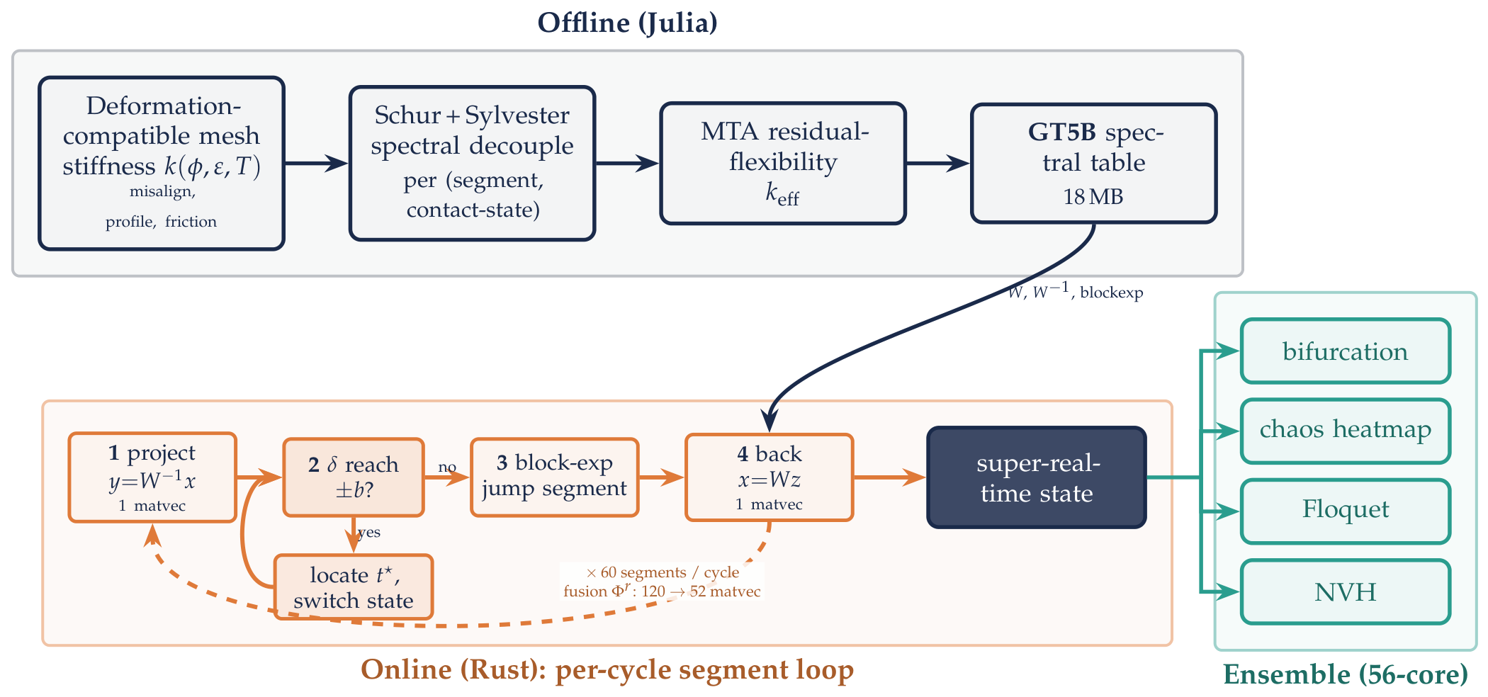
End-to-end pipeline. Offline (grey), a single deformation-compatible meshing model is decoupled per (segment, contact-state) into an 18 spectral table (GT5B). Online (amber), each mesh cycle sweeps its 60 segments through a four-step loop — project into spectral coordinates (, one matvec), test in closed form whether the deflection reaches the backlash edge , then either block-exponential jump the whole segment or locate the crossing time and switch contact state, and finally map back (, one matvec) — so a raw cycle costs 120 matvec, cut to 52 by segment fusion. The resulting super-real-time state feeds the 56-core branch (teal) that extracts bifurcation, chaos, Floquet, and NVH structure.
Figure A1.
End-to-end pipeline. Offline (grey), a single deformation-compatible meshing model is decoupled per (segment, contact-state) into an 18 spectral table (GT5B). Online (amber), each mesh cycle sweeps its 60 segments through a four-step loop — project into spectral coordinates (, one matvec), test in closed form whether the deflection reaches the backlash edge , then either block-exponential jump the whole segment or locate the crossing time and switch contact state, and finally map back (, one matvec) — so a raw cycle costs 120 matvec, cut to 52 by segment fusion. The resulting super-real-time state feeds the 56-core branch (teal) that extracts bifurcation, chaos, Floquet, and NVH structure.
The neutral direction.
The gear pair is rotationally symmetric: the direction that advances both wheels by a common rigid rotation leaves the mesh deflection unchanged (, hence ), so is structurally rank-deficient — and, physically, has a genuine nonzero component along , the nominal per-cycle advance. Periodicity must therefore be imposed only on the complement: we regularize with and project the -component out of the update. With this, Newton contracts cleanly even onto unstable orbits that no forward simulation could ever exhibit: the strong-rattle period-1 orbit converges from residual to within ten Newton iterations, a four-event rattling orbit with spanning both flanks. In the sparse-rattle regime the period-1 solve does not converge but the period-2 solve does — direct evidence that a flip (period-doubling) has already occurred there, consistent with its multiplier .
Ground truth versus Floquet: the grazing caveat.
Because shooting delivers the orbit and its monodromy independently, the linearized prediction can be tested against the true map. Kicking each converged orbit by (in reduced norm) and iterating the full nonlinear map gives per-return growth factors of for the sparse period-2 orbit — in reasonable accord with its unstable multiplier — but for the strong-rattle period-1 orbit whose dominant multiplier is , i.e. nominally stable. The first return already amplifies the kick from to : the perturbation does not evolve along the linearized flow at all, it changes which backlash crossings occur, and the orbit jumps to a different event sequence. This grazing-type sensitivity [40,44,45,46] is invisible to any monodromy computed along the unperturbed sequence, however carefully the saltation is handled. The practical rule we draw: in a nonsmooth system, Floquet multipliers certify stability only within the margin by which the event sequence itself is robust; near grazing, the Lyapunov exponent measured on the true map is the only honest sensitivity.
Design sensitivity: linearize per segment, not per cycle.
The same lesson governs parameter derivatives. A Fréchet derivative of the cycle map with respect to a design parameter (a stiffness scale, a misalignment) is unusable in the chaotic regime: the phase drift it must represent grows to within a cycle and the linearization leaves its validity ball. Differentiating at the segment level and re-fusing the perturbed propagators, by contrast, is accurate to — the segment is short enough for the linearization to hold, and the fusion recomposes exactly. Design sensitivity in this framework therefore inherits the same architecture as the solver itself: everything exact happens per segment; cycles are only ever products.
Appendix F. Computing Environment: Hardware and Software
Because the central claims of this paper are quantitative timings interpreted through a memory model, the hardware and software stack is part of the result and we specify it in full.
Hardware.
All timings were measured on a dual-socket workstation carrying two Intel Xeon E5-2680 v4 processors (Broadwell-EP, 14 cores each) for 28 physical cores and 56 hardware threads in total, at GHz base ( GHz turbo), organised as two NUMA nodes. The per-core cache hierarchy is 32 KB L1 data, 32 KB L1 instruction, and 256 KB L2, with a 35 MB L3 shared per socket; main memory is 32 GB of DDR4 (WSL2 exposes GB to the runtime). The cores implement AVX2 and FMA but not AVX-512. Two features of this machine are load-bearing for the argument. First, the 32 KB L1 data cache is exactly the threshold identified in Section 3.3: the dim-81 system operator ( KB) overflows it, which is why the matvec cost jumps at that dimension and why the fidelity knee sits near DOF . Second, the dual-socket NUMA topology sharpens the depth-versus-breadth wall of Figure 4: the 56-thread ensemble does not see 56 independent memory paths but two socket-level memory controllers, so independent trajectories contend for a shared and partly cross-socket bandwidth — the mechanism behind the measured (rather than ) ensemble speedup and its parallel efficiency. Figure A2 draws the hierarchy explicitly and places every working set of the solver on it: the reduced dim-41 operator (13 KB) inside each core’s L1, the raw dim-81 operator (52 KB) spilling into L2, the N40 spectral table (18 MB) resident in one socket’s L3, and the 8-table ensemble (144 MB) in DRAM behind the measured ≈32 GB/s aggregate-bandwidth ceiling of Figure 5b.
Figure A2.
Where the data lives and how it moves: the dual-socket memory hierarchy with the solver’s working sets mapped onto it. The reduced dim-41 operator (13 KB) is L1-resident per core; the raw dim-81 operator (52 KB) overflows L1 into L2; the full N40 spectral table (18 MB) is L3-resident on one socket; and the 8-table ensemble (144 MB) spills to DRAM, whose measured bandwidth (Fig. Figure 5b) saturates at ≈32 GB/s for the whole machine. Each matvec streams one operator column-wise through the FMA units, so a raw-N40 mesh cycle moves ≈6.3 MB of table — the kernel is a bandwidth workload, and every optimization in this paper (MTA reduction, segment fusion, spectral tables) is at bottom a scheme to move this traffic up the hierarchy.
Figure A2.
Where the data lives and how it moves: the dual-socket memory hierarchy with the solver’s working sets mapped onto it. The reduced dim-41 operator (13 KB) is L1-resident per core; the raw dim-81 operator (52 KB) overflows L1 into L2; the full N40 spectral table (18 MB) is L3-resident on one socket; and the 8-table ensemble (144 MB) spills to DRAM, whose measured bandwidth (Fig. Figure 5b) saturates at ≈32 GB/s for the whole machine. Each matvec streams one operator column-wise through the FMA units, so a raw-N40 mesh cycle moves ≈6.3 MB of table — the kernel is a bandwidth workload, and every optimization in this paper (MTA reduction, segment fusion, spectral tables) is at bottom a scheme to move this traffic up the hierarchy.
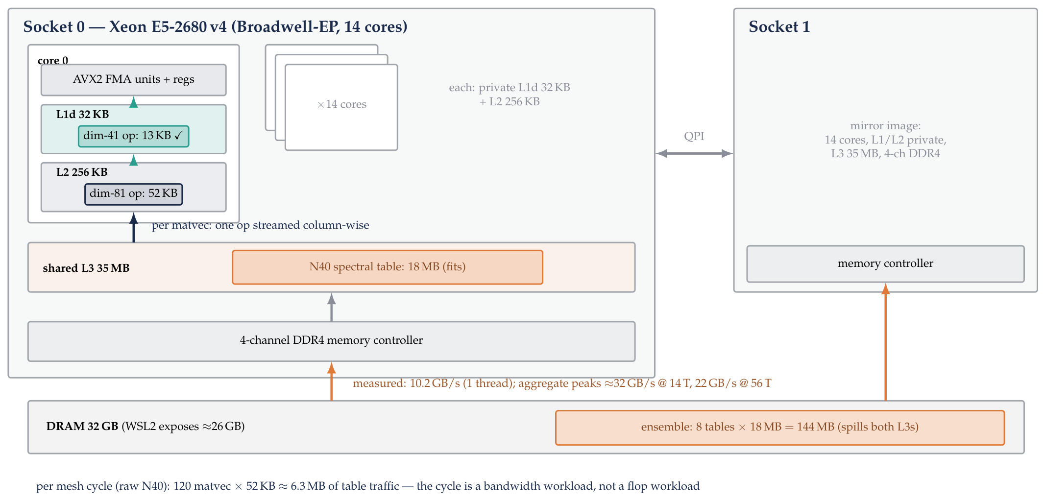
Software.
The runtime kernel is written in Rust (rustc/cargo ) and compiled with the release profile lto = true, codegen-units = 1, panic = "abort", and RUSTFLAGS = "-C target-cpu=native" so the segment matvec is vectorised to the machine’s AVX2/FMA width. Two low-level details matter for the reported numbers. Denormal floating-point operands — which arise in the near-zero modal coordinates produced by the inverse spectral basis and which otherwise trigger a microcode slowdown — are flushed to zero by setting the flush-to-zero and denormals-are-zero bits of the MXCSR control register (ldmxcsr | 0x8040) once at startup; and the per-segment propagator is written as a column-major saxpy over non-aliasing slices so that LLVM emits a clean vectorised inner loop. Thread-level parallelism for the ensemble sweeps (Figure 9, Figure 10) uses std::thread::scope with one worker per operating point over a shared, read-only spectral-table set. The offline table generation — the Schur ordering and Sylvester decoupling of Appendix A, the residual-flexibility MTA correction of Appendix C, and the segment-fusion products — is performed once in Julia () and serialised to a binary table that the Rust kernel memory-maps at load; no factorisation happens on the timed path. All reported wall-clock figures are single-run measurements on an otherwise idle machine with the frequency governor left at its default; because the kernel is memory-bandwidth-bound rather than clock-bound (its Roofline position is set by arithmetic intensity, not turbo residency), run-to-run variation is dominated by cache and NUMA placement rather than by core frequency.
References
- Shaw, S.; Holmes, P. A periodically forced piecewise linear oscillator. J. Sound. Vib. 1983. [Google Scholar] [CrossRef]
- Hongler, M.O.; Streit, L. On the origin of chaos in gearbox models. In Physica D: Nonlinear Phenomena; 1988. [Google Scholar] [CrossRef]
- THEODOSSIADES, S.; NATSIAVAS, S. NON-LINEAR DYNAMICS OF GEAR-PAIR SYSTEMS WITH PERIODIC STIFFNESS AND BACKLASH. J. Sound. Vib. 2000. [Google Scholar] [CrossRef]
- Theodossiades, S.; Natsiavas, S. Periodic and chaotic dynamics of motor-driven gear-pair systems with backlash. In Chaos, Solitons & Fractals; 2001. [Google Scholar] [CrossRef]
- Guo, D.; Ning, Q.; Ge, S.; Wang, Y.; Zhou, Y.; Zhou, Y.; Shi, X. Nonlinear characteristic analysis of gear rattle based on refined dynamic model. In Nonlinear Dynamics; 2022. [Google Scholar] [CrossRef]
- Donmez, A.; Kahraman, A. An experimental and theoretical investigation of the influence of backlash on gear train vibro-impacts and rattle noise. Proc. Inst. Mech. Eng. Part K. J. Multi-Body Dyn. 2023. [Google Scholar] [CrossRef]
- Wang, Y.; Zhu, G.; Zhang, F. Powertrain control parameter optimisation using HIL simulations of a heavy-duty vehicle. Int. J. Powertrains 2013. [Google Scholar] [CrossRef]
- Archut, J.L.; Corves, B. Systematic mapping of methods for real-time capable multibody simulation of road vehicles using PRISMA. In Multibody System Dynamics; 2026. [Google Scholar] [CrossRef]
- Ding, R.; Li, J. Nonlinear finite-time Lyapunov exponent and predictability. Phys. Lett. A 2007. [Google Scholar] [CrossRef]
- Angelidis, A.K.; Makris, G.C.; Ioannidis, E.; Antoniou, I.E.; Bratsas, C. How Far Can We Trust Chaos? Extending the Horizon of Predictability. Mathematics 2025. [Google Scholar] [CrossRef]
- Hochbruck, M.; Ostermann, A. Exponential integrators. Acta Numer. 2010. [Google Scholar] [CrossRef]
- Cox, S.; Matthews, P. Exponential Time Differencing for Stiff Systems. J. Comput. Phys. 2002. [Google Scholar] [CrossRef]
- Zhuang, H.; Yu, W.; Weng, S.H.; Kang, I.; Lin, J.H.; Zhang, X.; Coutts, R.; Cheng, C.K. Simulation Algorithms with Exponential Integration for Time-Domain Analysis of Large-Scale Power Delivery Networks. IEEE Transactions on Computer-Aided Design of Integrated Circuits and Systems, 2016. [Google Scholar] [CrossRef]
- Acary, V.; Brogliato, B. Numerical Methods for Nonsmooth Dynamical Systems. In Lecture Notes in Applied and Computational Mechanics; Springer, 2008. [Google Scholar] [CrossRef]
- Leine, R.I.; Nijmeijer, H. Dynamics and Bifurcations of Non-Smooth Mechanical Systems. In Lecture Notes in Applied and Computational Mechanics; Springer, 2004; vol. 18. [Google Scholar] [CrossRef]
- Kong, N.J.; Payne, J.J.; Zhu, J.; Johnson, A.M. Saltation Matrices: The Essential Tool for Linearizing Hybrid Dynamical Systems. arXiv. 2023. Available online: https://arxiv.org/abs/2306.06862.
- (LBNL), S.W. The Roofline Model: Visualizing and Optimizing Performance. Lawrence Berkeley National Laboratory. Available online: https://amcr.lbl.gov/departments/computer-science-department/ppan/roofline-performance-model/.
- Zhang, H.; Zhang, H. Solving time-varying mesh stiffness of spur gears based on improved potential energy method. J. Mech. Eng. Autom. Control Syst. 2024. [Google Scholar] [CrossRef]
- Hou, J.; Yang, S.; Li, Q.; Liu, Y.; Wang, J. Mesh stiffness calculation and vibration analysis of the spur gear pair with tooth crack, considering the misalignment between the base and root circles. Int. J. Mech. Syst. Dyn. 2021. [Google Scholar] [CrossRef]
- Ambaye, G.A.; Lemu, H.G. Effect of Backlash on Transmission Error and Time Varying Mesh Stiffness. In Lecture Notes in Electrical Engineering; 2021. [Google Scholar] [CrossRef]
- Rixen, D. Generalized mode acceleration methods and modal truncation augmentation. 19th AIAA Applied Aerodynamics Conference, 2001. [Google Scholar] [CrossRef]
- Ding, Z.; Li, H.; Zou, G.; Kong, J. Considering higher-order effects of residual attachment modes in free-interface component mode synthesis method for non-classically damped systems. J. Sound. Vib. 2020. [Google Scholar] [CrossRef]
- school; NASA CR), K. Dynamic Analysis of Geared Rotors by Finite Elements. NASA Technical Reports Server. Available online: https://ntrs.nasa.gov/api/citations/19900006970/downloads/19900006970.pdf.
- Gruber, F.M.; Rixen, D.J. Dual Craig-Bampton component mode synthesis method for model order reduction of nonclassically damped linear systems. Mech. Syst. Signal Process. 2018. [Google Scholar] [CrossRef]
- Hernández Rocha, A.; Zanette, D.H.; Wiercigroch, M. Semi-analytical method to study piecewise linear oscillators. Commun. Nonlinear Sci. Numer. Simul. 2023. [Google Scholar] [CrossRef]
- Shripad, K.M.R.; Sundar, S. Semi-analytical solution for a system with clearance nonlinearity and periodic excitation. In Nonlinear Dynamics; 2023. [Google Scholar] [CrossRef]
- Haddouni, M.; Acary, V.; Garreau, S.; Beley, J.D.; Brogliato, B. Comparison of several formulations and integration methods for the resolution of DAEs formulations in event-driven simulation of nonsmooth frictionless multibody dynamics. Multibody Syst. Dyn. 2017. [Google Scholar] [CrossRef]
- Nurkanović, A.; Sperl, M.; Albrecht, S.; Diehl, M. Finite Elements with Switch Detection for direct optimal control of nonsmooth systems. In Numerische Mathematik; 2024. [Google Scholar] [CrossRef]
- Saito, A.; Tanaka, M. Data-driven model order reduction for structures with piecewise linear nonlinearity using dynamic mode decomposition. arXiv. 2026. Available online: https://arxiv.org/pdf/2603.17423.
- Louboutin, M.; Lange, M.; Herrmann, F.; Kukreja, N.; Gorman, G. Performance prediction of finite-difference solvers for different computer architectures. arXiv. 2016. Available online: https://arxiv.org/pdf/1608.03984.
- Liao, S. On the reliability of computed chaotic solutions of nonlinear differential equations. Tellus A, 2009. [Google Scholar]
- MASON, J.F.; PIIROINEN, P.T.; WILSON, R.E.; HOMER, M.E. BASINS OF ATTRACTION IN NONSMOOTH MODELS OF GEAR RATTLE. Int. J. Bifurc. Chaos 2009. [Google Scholar] [CrossRef]
- Niemeyer, K.E.; Sung, C.J. GPU-Based Parallel Integration of Large Numbers of Independent ODE Systems. arXiv. 2016. Available online: https://arxiv.org/pdf/1611.02274.
- Hegedus, F. MPGOS: Massively-Parallel-GPU-ODE-Solver for large numbers of independent ODE systems. Software (GitHub). Available online: https://github.com/FerencHegedus/Massively-Parallel-GPU-ODE-Solver.
- Nagy, D.; Plavecz, L.; Hegedűs, F. The art of solving a large number of non-stiff, low-dimensional ordinary differential equation systems on GPUs and CPUs. Commun. Nonlinear Sci. Numer. Simul. 2022. [Google Scholar] [CrossRef]
- Intel. Optimize Memory-bound Applications with GPU Roofline. Intel oneAPI Optimization Guide, 2024. Available online: https://www.intel.com/content/www/us/en/docs/oneapi/optimization-guide-gpu/2024-1/advisor-roofline-analysis.html.
- SÁNCHEZ, J.; NET, M. ON THE MULTIPLE SHOOTING CONTINUATION OF PERIODIC ORBITS BY NEWTON–KRYLOV METHODS. Int. J. Bifurc. Chaos 2010. [Google Scholar] [CrossRef]
- Dankowicz, H.; Schilder, F. Recipes for Continuation; SIAM, 2013. [Google Scholar] [CrossRef]
- Iklodi, Z.; Dombovari, Z. Bifurcation analysis of piecewise-smooth engineering systems with delays through numeric continuation of periodic orbits. In Nonlinear Dynamics; 2024. [Google Scholar] [CrossRef]
- Ghosh, I.; Simpson, D.J.W. The VIVID function for numerically continuing periodic orbits arising from grazing bifurcations of hybrid dynamical systems. arXiv. 2025. Available online: https://arxiv.org/pdf/2510.16218.
- Lai, C.; Chen, Y. On the Computation of Floquet Multipliers for Periodic Solution in Piecewise-smooth Dynamical System. J. Phys. Conf. Ser. 2024. [Google Scholar] [CrossRef]
- di Bernardo, M.; Budd, C.J.; Champneys, A.R.; Kowalczyk, P.; Nordmark, A.B.; Tost, G.O.; Piiroinen, P.T. Bifurcations in Nonsmooth Dynamical Systems. SIAM Rev. 2008. [Google Scholar] [CrossRef]
- Yin, S.; Ji, J.; Deng, S.; Wen, G. Degenerate grazing bifurcations in a three-degree-of-freedom impact oscillator. In Nonlinear Dynamics; 2019. [Google Scholar] [CrossRef]
- Kryzhevich, S. Grazing bifurcation and chaotic oscillations of vibro-impact systems with one degree of freedom. J. Appl. Math. Mech. 2008. [Google Scholar] [CrossRef]
- Jiang, H.; Chong, A.S.; Ueda, Y.; Wiercigroch, M. Grazing-induced bifurcations in impact oscillators with elastic and rigid constraints. Int. J. Mech. Sci. 2017. [Google Scholar] [CrossRef]
- Xu, J.; Li, Q.; Wang, N. Existence and stability of the grazing periodic trajectory in a two-degree-of-freedom vibro-impact system. Appl. Math. Comput. 2011. [Google Scholar] [CrossRef]
- Loffeld, J.; Tokman, M. Comparative performance of exponential, implicit, and explicit integrators for stiff systems of ODEs. J. Comput. Appl. Math. 2013. [Google Scholar] [CrossRef]
- Ros, J.; Plaza, A.; Iriarte, X.; Pintor, J.M. Symbolic Multibody Methods for Real-Time Simulation of Railway Vehicles. arXiv. 2017. Available online: https://arxiv.org/pdf/1706.01657.
Figure 1.
The layered real-time ceiling: each increment in system character lowers the achievable wall-clock speed-up by orders of magnitude, from a skippable linear semigroup (, no ceiling) through a event bound to a high-dimensional Roofline regime where memory-aware retiling plus fusion lifts a raw baseline across real-time to — proving that every ceiling left of the chaotic Lyapunov wall is an engineering limit that can be optimized, while the wall itself is physical and forces a shift from simulating trajectories to computing structure (conceptual map: dots mark measured ratios, connecting risers are schematic).
Figure 1.
The layered real-time ceiling: each increment in system character lowers the achievable wall-clock speed-up by orders of magnitude, from a skippable linear semigroup (, no ceiling) through a event bound to a high-dimensional Roofline regime where memory-aware retiling plus fusion lifts a raw baseline across real-time to — proving that every ceiling left of the chaotic Lyapunov wall is an engineering limit that can be optimized, while the wall itself is physical and forces a shift from simulating trajectories to computing structure (conceptual map: dots mark measured ratios, connecting risers are schematic).
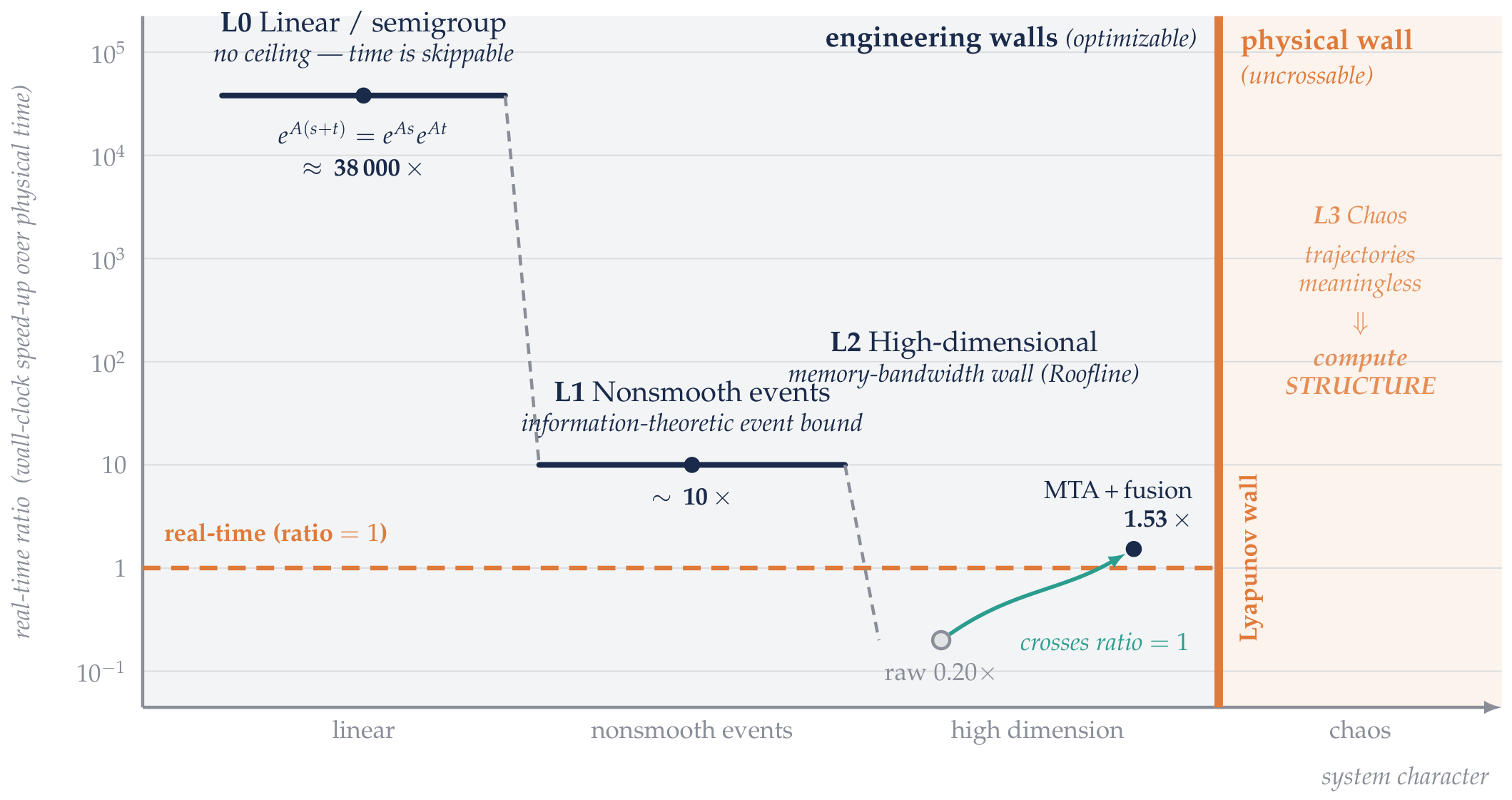
Figure 2.
What the five test cases actually are, in one row. Every tier is driven by the same high-fidelity mesh-stiffness engine (top bar): the tooth compliance is computed by the improved potential-energy method [18,19] — bending, shear, axial and Hertzian-contact energies summed along the instantaneous contact lines — so the stiffness varies with mesh angle through the engagement cycle; shaft misalignment enters as a single effective angular deviation that can unload part of the flank (partial contact, with the tangent stiffness and load centre shifting accordingly), and the transmitted torque T and profile modification are resolved by deformation compatibility, giving one tabulated [20]. Fidelity is then added left to right. Tier 1: two rigid discs on rigid mounts, torsional DOF only. Tier 2: adds gear-body translations on bearing springs . Tier 3: adds the tilt/load-centre pair , tooth friction , and closes the misalignment loop through the table. Tier 4: mounts each bearing on a sprung pedestal seat (two-stage isolation). Tier 5: replaces rigid shafts by modal flexible shafts ( retained modes, state dimension 81) and opens the three-state backlash gap — the most complex configuration of Table 4. The small-step real-time factors below each panel are those of Table 1.
Figure 2.
What the five test cases actually are, in one row. Every tier is driven by the same high-fidelity mesh-stiffness engine (top bar): the tooth compliance is computed by the improved potential-energy method [18,19] — bending, shear, axial and Hertzian-contact energies summed along the instantaneous contact lines — so the stiffness varies with mesh angle through the engagement cycle; shaft misalignment enters as a single effective angular deviation that can unload part of the flank (partial contact, with the tangent stiffness and load centre shifting accordingly), and the transmitted torque T and profile modification are resolved by deformation compatibility, giving one tabulated [20]. Fidelity is then added left to right. Tier 1: two rigid discs on rigid mounts, torsional DOF only. Tier 2: adds gear-body translations on bearing springs . Tier 3: adds the tilt/load-centre pair , tooth friction , and closes the misalignment loop through the table. Tier 4: mounts each bearing on a sprung pedestal seat (two-stage isolation). Tier 5: replaces rigid shafts by modal flexible shafts ( retained modes, state dimension 81) and opens the three-state backlash gap — the most complex configuration of Table 4. The small-step real-time factors below each panel are those of Table 1.
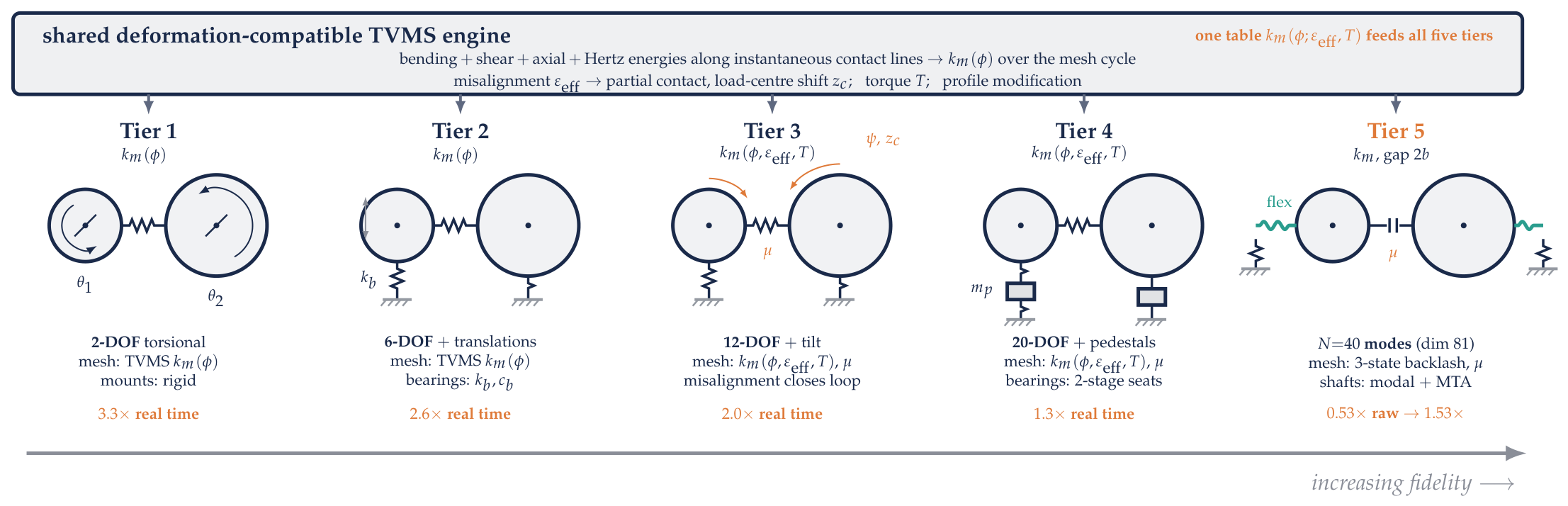
Figure 3.
MTA (into L1) plus segment fusion (matvec ) carry the hardest configuration ( DOF, near-resonance ) from to super-real-time at fixed fidelity, crossing the real-time wall.
Figure 3.
MTA (into L1) plus segment fusion (matvec ) carry the hardest configuration ( DOF, near-resonance ) from to super-real-time at fixed fidelity, crossing the real-time wall.
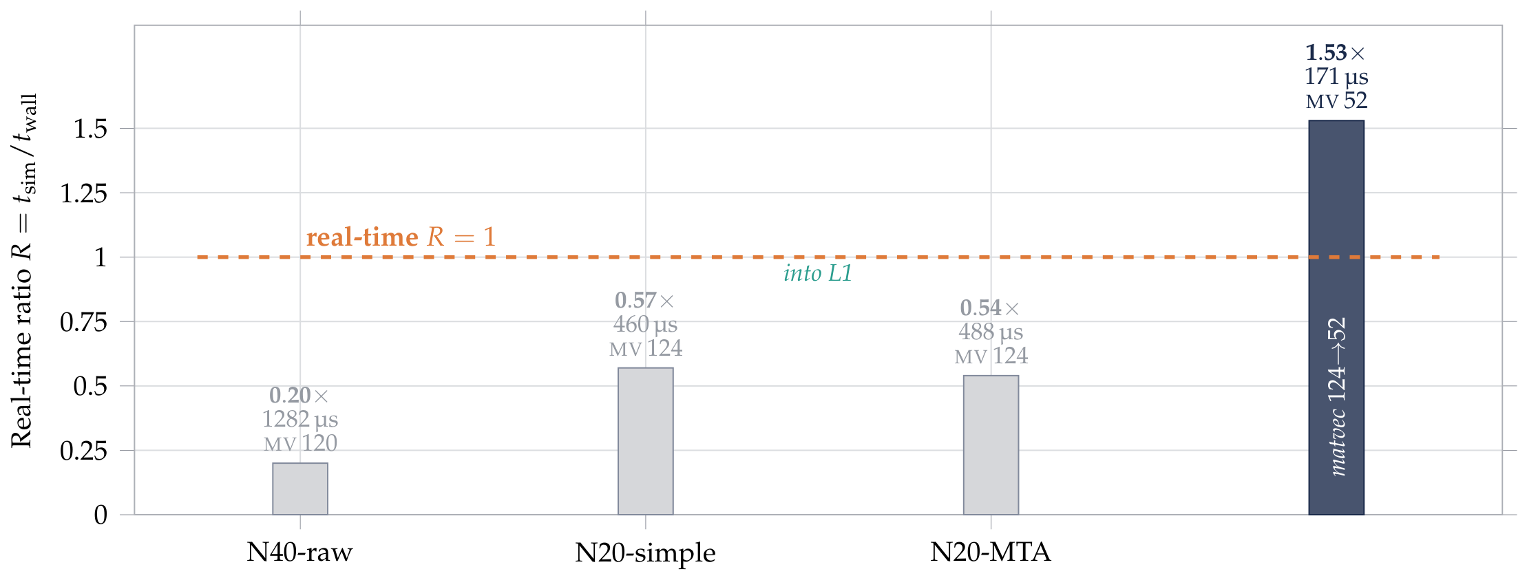
Figure 4.
Both single-trajectory depth and ensemble breadth are throttled by one bandwidth wall: per-matvec cost jumps ( →) exactly when W outgrows the 32 L1 cache—the matrix is whereas the at still fits (crossing near )—and the same limit caps ensemble scaling at against an ideal ( efficiency); the dashed line through the three measured points is a reference only, not a fit.
Figure 4.
Both single-trajectory depth and ensemble breadth are throttled by one bandwidth wall: per-matvec cost jumps ( →) exactly when W outgrows the 32 L1 cache—the matrix is whereas the at still fits (crossing near )—and the same limit caps ensemble scaling at against an ideal ( efficiency); the dashed line through the three measured points is a reference only, not a fit.
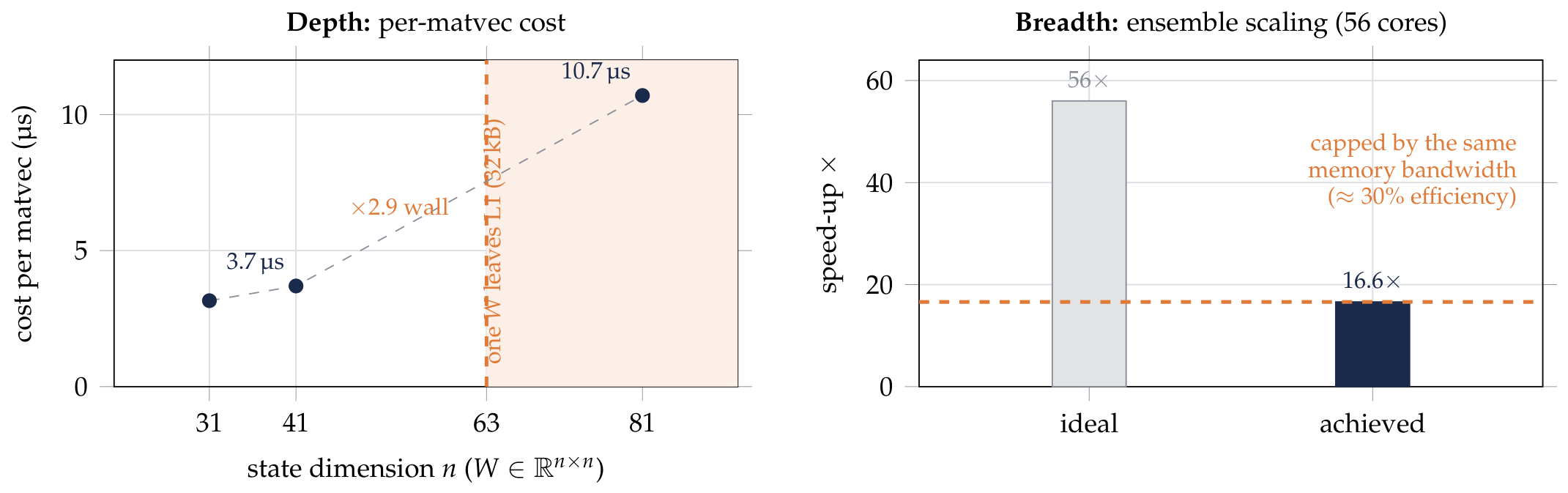
Figure 5.
Direct measurement of the memory system under the production kernel (PMU counters are unavailable under WSL2, so the hierarchy is characterized by microbenchmark). (a) the exact solver matvec (matvec_cols_into) applied to a rotating set of operators: cost is flat while the rotating working set — the spectral-table footprint — stays inside the 35 MB socket L3, then jumps (dim 81: s) once it spills to DRAM. The cliff tracks the table, not the single operator. (b) aggregate streaming read bandwidth saturates at ≈32 GB/s with only 14 threads — barely one core’s 10.2 GB/s — and decreases to 22 GB/s at 56 threads under NUMA and oversubscription pressure. (c) thread scaling of the full spectral solver on a shared table saturates at 25– on 56 threads, and the harder 8-table atlas workload of Figure 9 at : depth and breadth are throttled by the same measured bandwidth ceiling of panel (b).
Figure 5.
Direct measurement of the memory system under the production kernel (PMU counters are unavailable under WSL2, so the hierarchy is characterized by microbenchmark). (a) the exact solver matvec (matvec_cols_into) applied to a rotating set of operators: cost is flat while the rotating working set — the spectral-table footprint — stays inside the 35 MB socket L3, then jumps (dim 81: s) once it spills to DRAM. The cliff tracks the table, not the single operator. (b) aggregate streaming read bandwidth saturates at ≈32 GB/s with only 14 threads — barely one core’s 10.2 GB/s — and decreases to 22 GB/s at 56 threads under NUMA and oversubscription pressure. (c) thread scaling of the full spectral solver on a shared table saturates at 25– on 56 threads, and the harder 8-table atlas workload of Figure 9 at : depth and breadth are throttled by the same measured bandwidth ceiling of panel (b).
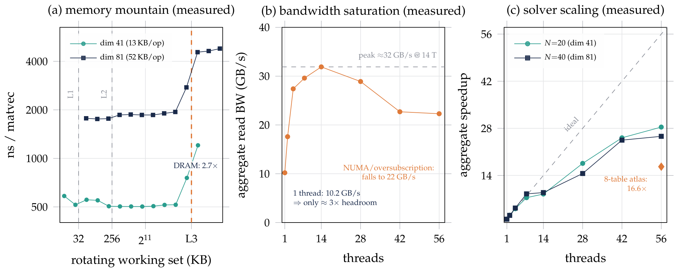
Figure 6.
Exact fused -map propagation is faster ( vs. ) and more accurate ( vs. ) than a tuned adaptive integrator (Vern7@; Tsit5 and Rodas5P occupy the same upper-right region), proving the speed is not bought with accuracy; both markers are measured points and down-left is better.
Figure 6.
Exact fused -map propagation is faster ( vs. ) and more accurate ( vs. ) than a tuned adaptive integrator (Vern7@; Tsit5 and Rodas5P occupy the same upper-right region), proving the speed is not bought with accuracy; both markers are measured points and down-left is better.
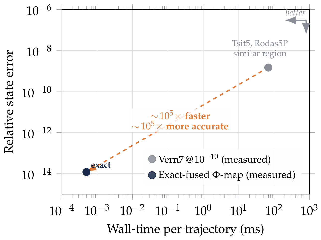
Figure 7.
The largest Lyapunov exponent , fixed by the two measured separation points, sets a predictability wall at rattle cycles that no solver speed can push back — a accuracy gain moves the wall by only cycles.
Figure 7.
The largest Lyapunov exponent , fixed by the two measured separation points, sets a predictability wall at rattle cycles that no solver speed can push back — a accuracy gain moves the wall by only cycles.
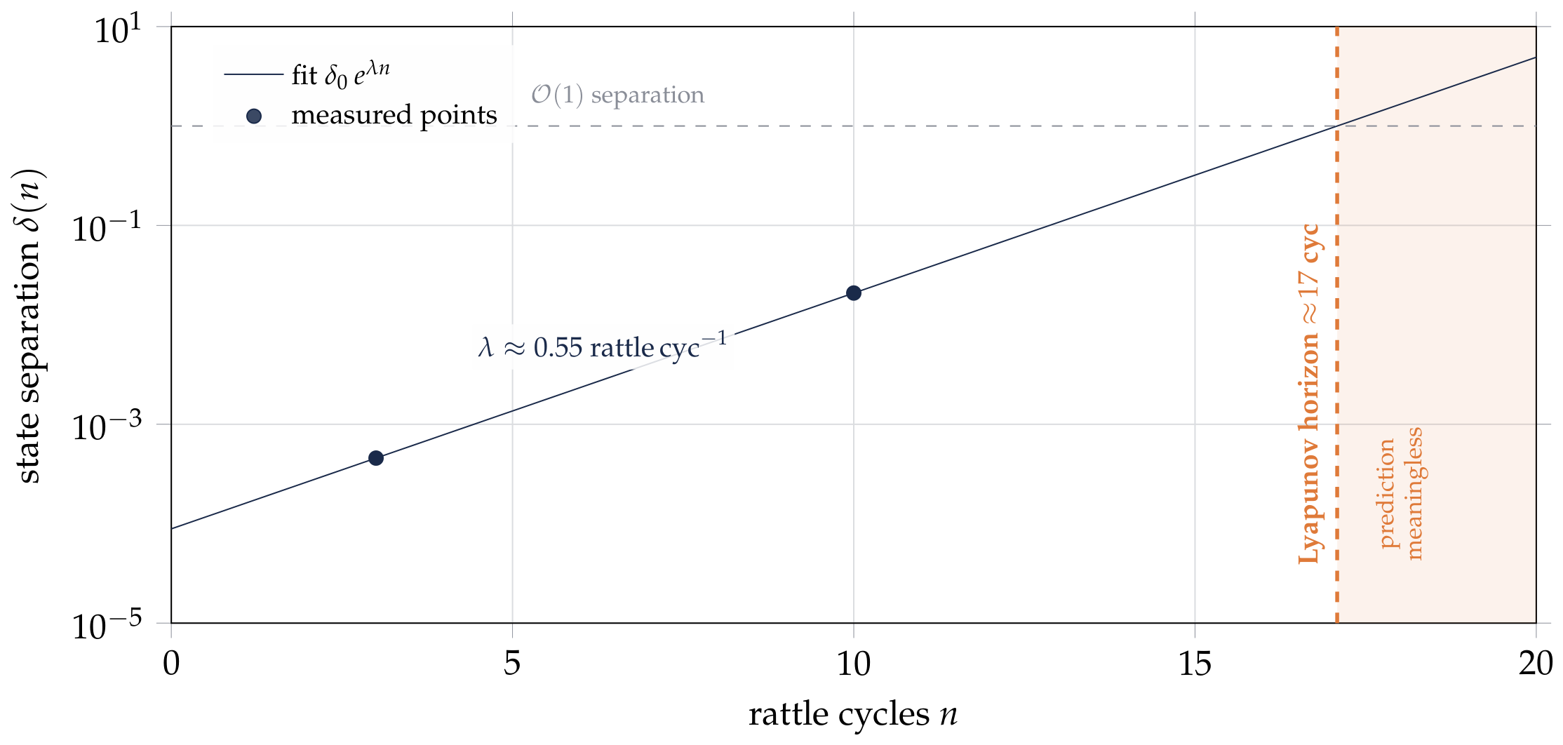
Figure 8.
The trajectories-give-way-to-structure crossover, measured on the fully resolved flexible model (, dim 81). A perturbed twin’s normalized state separation (R the attractor radius) rises to saturation by a predictability horizon mesh cycles (Benettin exponent cyc, order-one and consistent with the 6-DOF skeleton). Over the same lengths, the relative standard error of a time-averaged structural observable (mean contact force) falls as , from toward by 400 cycles. The two cross near : to the left the pointwise orbit is the better-determined object, to the right the statistical structure is — so past the horizon the real-time budget is better spent on structure than on one more decorrelating trajectory.
Figure 8.
The trajectories-give-way-to-structure crossover, measured on the fully resolved flexible model (, dim 81). A perturbed twin’s normalized state separation (R the attractor radius) rises to saturation by a predictability horizon mesh cycles (Benettin exponent cyc, order-one and consistent with the 6-DOF skeleton). Over the same lengths, the relative standard error of a time-averaged structural observable (mean contact force) falls as , from toward by 400 cycles. The two cross near : to the left the pointwise orbit is the better-determined object, to the right the statistical structure is — so past the horizon the real-time budget is better spent on structure than on one more decorrelating trajectory.
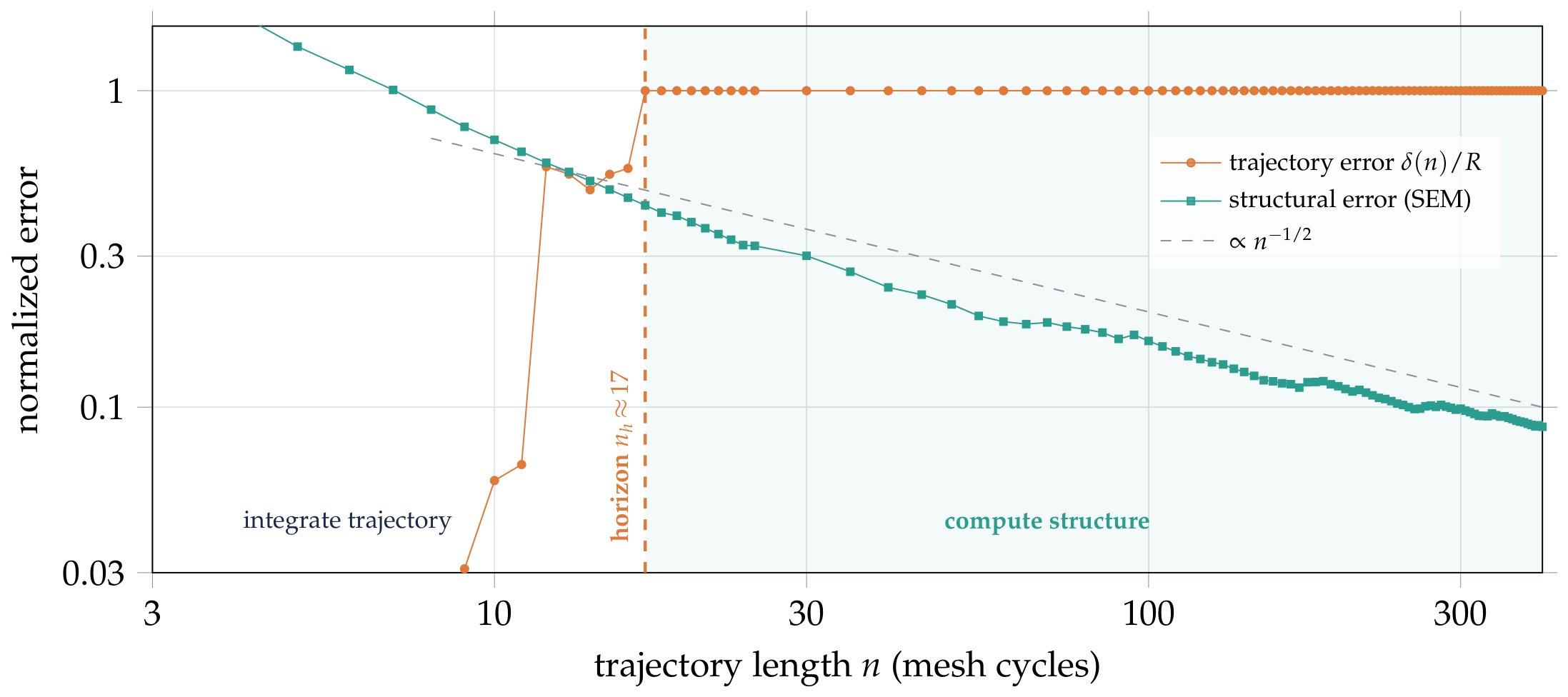
Figure 9.
A real-time-computed chaos atlas of the rattling gear pair: across the entire wide- operating grid every point is chaotic (, 0 of 80 stable period-1 orbits), the largest exponent peaking at per mesh cycle at under 16 load (×) and thinning to only along the high- edge and the low-/high-load corner — the whole map recomputed on 56 cores in ( over serial via a shared ARC table), the “structure” that stays computable long past the per-trajectory Lyapunov wall.
Figure 9.
A real-time-computed chaos atlas of the rattling gear pair: across the entire wide- operating grid every point is chaotic (, 0 of 80 stable period-1 orbits), the largest exponent peaking at per mesh cycle at under 16 load (×) and thinning to only along the high- edge and the low-/high-load corner — the whole map recomputed on 56 cores in ( over serial via a shared ARC table), the “structure” that stays computable long past the per-trajectory Lyapunov wall.
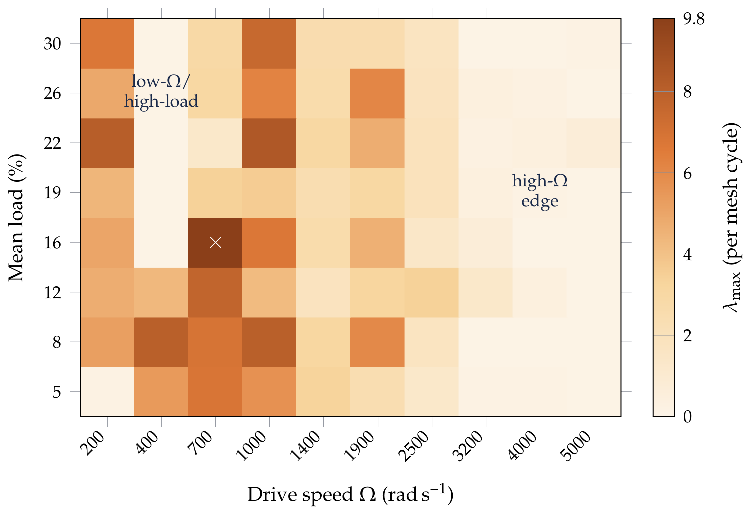
Figure 10.
Nominal-speed sweep of the flexible rattle model. (a) Poincaré section of the mesh deflection (sampled once per mesh cycle after transient) against the speed ratio : a densely filled band signals chaos, which dominates the range. (b) the largest Lyapunov exponent over the same sweep stays well above zero except in a narrow near-periodic window at , where it dips to and the Poincaré set collapses to a thin band. An explicit 128-trajectory multistability probe (32 stratified initial conditions at the window centre, both shoulders, and a control point) found every trajectory chaotic (): the window is weak chaos, not a periodic island, and no coexisting attractor exists.
Figure 10.
Nominal-speed sweep of the flexible rattle model. (a) Poincaré section of the mesh deflection (sampled once per mesh cycle after transient) against the speed ratio : a densely filled band signals chaos, which dominates the range. (b) the largest Lyapunov exponent over the same sweep stays well above zero except in a narrow near-periodic window at , where it dips to and the Poincaré set collapses to a thin band. An explicit 128-trajectory multistability probe (32 stratified initial conditions at the window centre, both shoulders, and a control point) found every trajectory chaotic (): the window is weak chaos, not a periodic island, and no coexisting attractor exists.
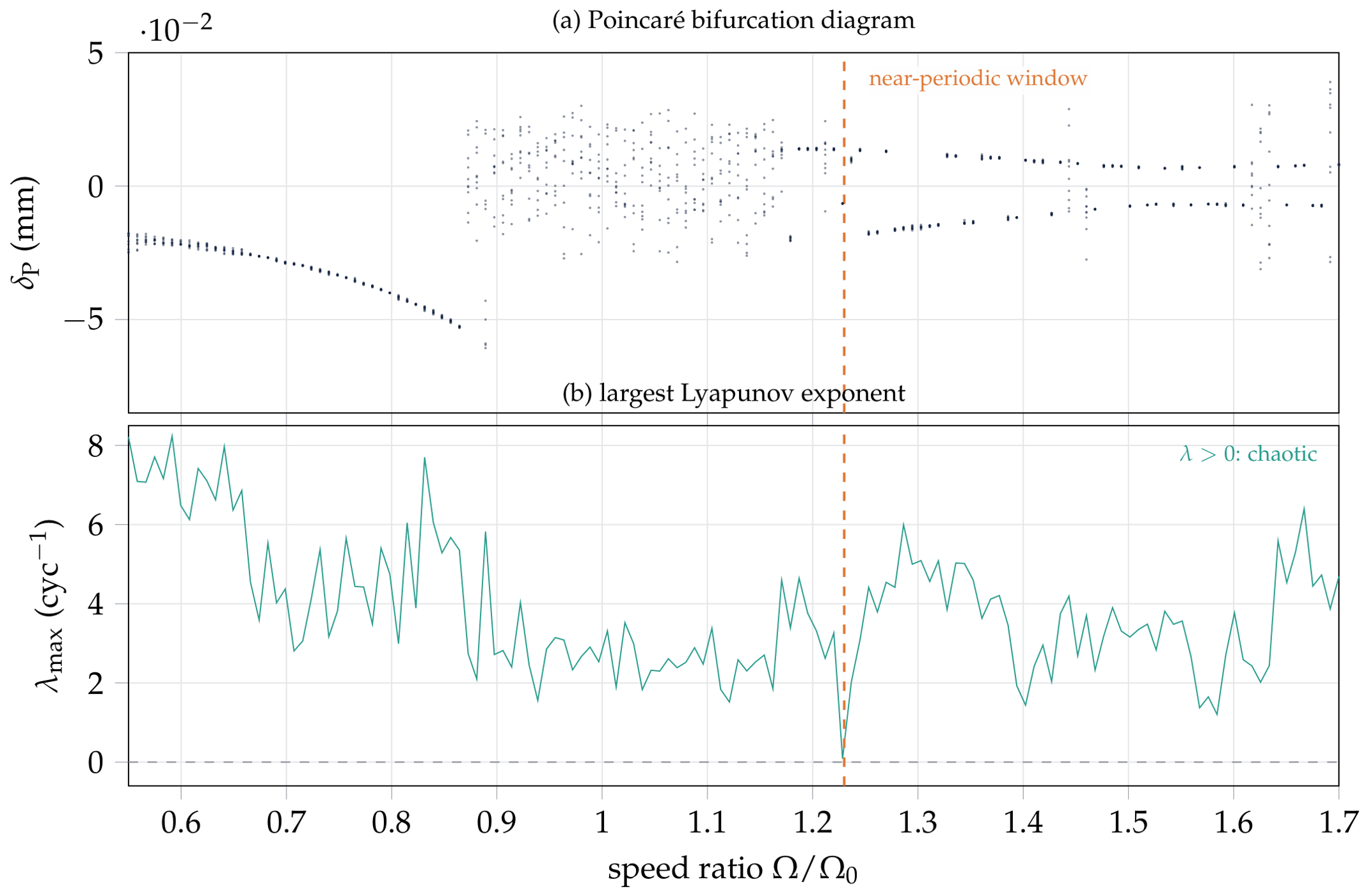
Figure 11.
Where periodic orbits exist, the Floquet spectrum of the 6-DOF strong-rattle period-1 skeleton pins the bifurcation type: the dominant complex pair at () sits only 0.028 inside the unit circle, a Neimark–Sacker onset toward quasiperiodic rattle, while a period-2 branch already carries a real multiplier at (flip/unstable); the neutral pair lies at and the markers are the remaining computed multipliers (magnitude fixed at , phase unconstrained).
Figure 11.
Where periodic orbits exist, the Floquet spectrum of the 6-DOF strong-rattle period-1 skeleton pins the bifurcation type: the dominant complex pair at () sits only 0.028 inside the unit circle, a Neimark–Sacker onset toward quasiperiodic rattle, while a period-2 branch already carries a real multiplier at (flip/unstable); the neutral pair lies at and the markers are the remaining computed multipliers (magnitude fixed at , phase unconstrained).
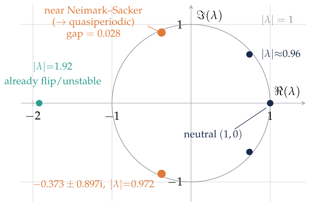
Figure 12.
The engineering NVH signature falls out of the same real-time rattle solver: a non-Gaussian DTE waveform with peak-to-peak 60 over RMS 13 (pp/RMS , an impact signature), whose fundamental equals the STE excitation above a chaotic broadband floor, while the contact-force peak climbs from at 5 load to at 30. Panel (a) is schematic (statistics only); higher-harmonic heights are illustrative, whereas , the DTE statistics and both contact-force points are measured.
Figure 12.
The engineering NVH signature falls out of the same real-time rattle solver: a non-Gaussian DTE waveform with peak-to-peak 60 over RMS 13 (pp/RMS , an impact signature), whose fundamental equals the STE excitation above a chaotic broadband floor, while the contact-force peak climbs from at 5 load to at 30. Panel (a) is schematic (statistics only); higher-harmonic heights are illustrative, whereas , the DTE statistics and both contact-force points are measured.
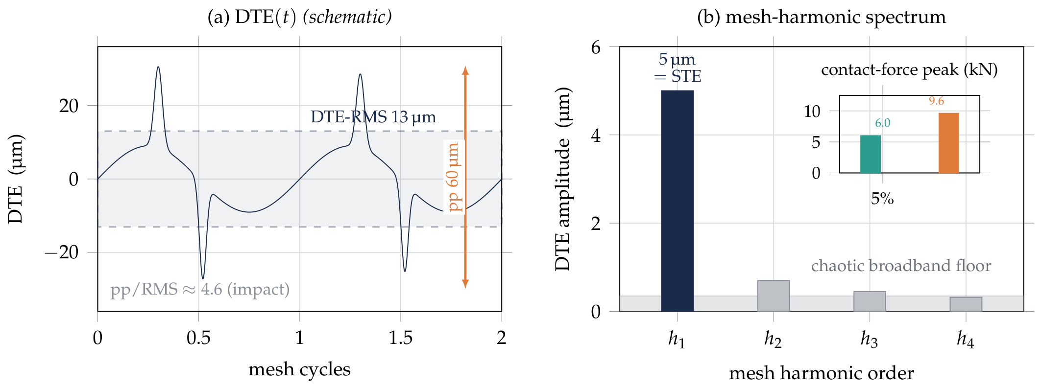
Figure 13.
Chaotic-rattle signatures at the strong-rattle operating point (flexible model). (a) phase portrait of mesh deflection versus its rate, (grey cloud), with the once-per-cycle Poincaré section overlaid (orange): the orbit fills a bounded region and crosses the backlash band repeatedly, and the Poincaré set is a fractal-like scatter rather than a finite point set — the geometric signature of chaos. (b) the corresponding power spectra of the DTE and contact force show the mesh fundamental and its harmonics riding on a broadband, subharmonic-rich floor, the spectral signature of the same non-periodic motion.
Figure 13.
Chaotic-rattle signatures at the strong-rattle operating point (flexible model). (a) phase portrait of mesh deflection versus its rate, (grey cloud), with the once-per-cycle Poincaré section overlaid (orange): the orbit fills a bounded region and crosses the backlash band repeatedly, and the Poincaré set is a fractal-like scatter rather than a finite point set — the geometric signature of chaos. (b) the corresponding power spectra of the DTE and contact force show the mesh fundamental and its harmonics riding on a broadband, subharmonic-rich floor, the spectral signature of the same non-periodic motion.
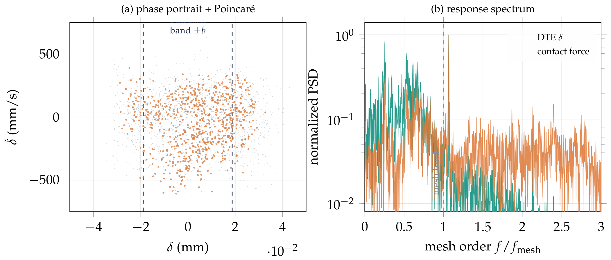
Figure 14.
Progressive expansion of the flexible model from to 40 retained modes (state dimension ). (a) the single-cycle DTE waveform sharpens and gains amplitude as modes are added, the response converging toward the curve. (b) the impact-severity metric converges quickly (m), but the largest Lyapunov exponent does not: coarse truncations over-estimate the chaos ( at ) and only the resolved model settles to per mesh cycle, in line with the reduced 6-DOF skeleton ( per rattle cycle). Enough degrees of freedom are needed not merely for amplitude fidelity but to avoid a spurious over-prediction of sensitivity.
Figure 14.
Progressive expansion of the flexible model from to 40 retained modes (state dimension ). (a) the single-cycle DTE waveform sharpens and gains amplitude as modes are added, the response converging toward the curve. (b) the impact-severity metric converges quickly (m), but the largest Lyapunov exponent does not: coarse truncations over-estimate the chaos ( at ) and only the resolved model settles to per mesh cycle, in line with the reduced 6-DOF skeleton ( per rattle cycle). Enough degrees of freedom are needed not merely for amplitude fidelity but to avoid a spurious over-prediction of sensitivity.
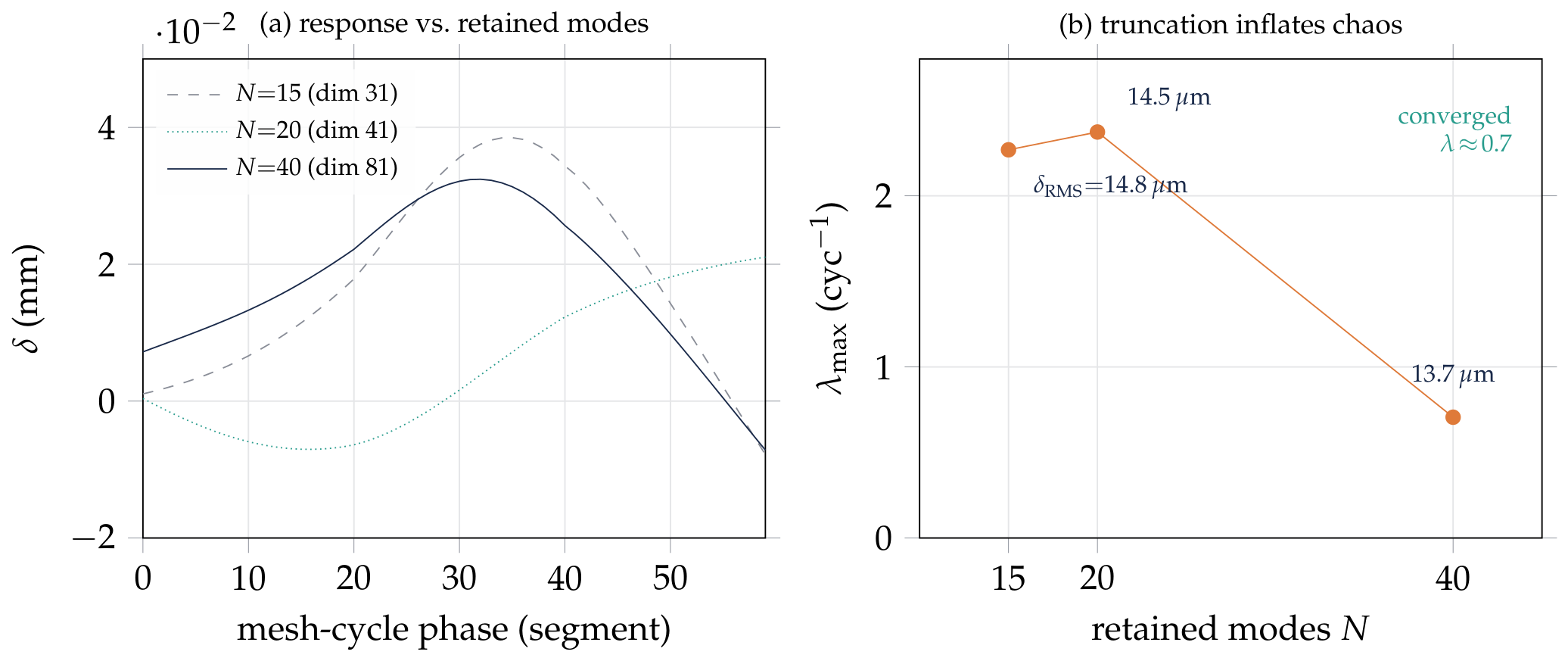
Table 1.
The real-time ratio degrades monotonically with model order as the state matrix crosses cache levels—holding above unity through Tier 4 (, 20 DOF) and falling to once the flexible Tier 5 spills to memory—while constant-contact fusion escapes the ladder entirely via the semigroup, reaching thousands× real time.
Table 1.
The real-time ratio degrades monotonically with model order as the state matrix crosses cache levels—holding above unity through Tier 4 (, 20 DOF) and falling to once the flexible Tier 5 spills to memory—while constant-contact fusion escapes the ladder entirely via the semigroup, reaching thousands× real time.
| Model | DOF | ns/step | Real-time | Limiting wall |
|---|---|---|---|---|
| (small-step) | ratio | |||
| Tier 1 | 2 | 30 | compute | |
| Tier 2 | 6 | 38 | compute | |
| Tier 3 | 12 | 49 | compute | |
| Tier 4 | 20 | 79 | compute | |
| real-time floor crossed below — structure, not trajectory, from here | ||||
| Tier 5 (flex) | 40 modal | 189 | 0.53× | memory |
| Tier 1–3 const.-contact fusion | — | — | thousands | semigroup (time skipped) |
Table 2.
Closed-form spectral event location cuts matvec/cycle to 74 (strong, ) and 29 (sparse, ), reversing the V2 certificate solver into super-real-time playback at a 7e-15 cross-check residual. V0, the naive small-step reference integrator, has no event-location structure to count and serves throughout only as the cross-check oracle.
Table 2.
Closed-form spectral event location cuts matvec/cycle to 74 (strong, ) and 29 (sparse, ), reversing the V2 certificate solver into super-real-time playback at a 7e-15 cross-check residual. V0, the naive small-step reference integrator, has no event-location structure to count and serves throughout only as the cross-check oracle.
| Method | matvec/cycle | wall () |
real-time | note |
|---|---|---|---|---|
| Strong rattle, | ||||
| V1 dyadic + bisection | 371 | 48 | baseline | |
| V2 certificate + Hermite | 193 | 31 | matvec | |
| V3 spectral closed-form | 74 | 33 | 0-matvec event locate | |
| Sparse contact, | ||||
| V2 sparse | 77.7 | 17.2 | – | |
| V3 sparse | 29.1 | 14.6 | cross-check 7e-15 | |
Table 3.
MTA (into L1) then segment fusion (matvec ) reach super-real-time at unchanged fidelity ().
Table 3.
MTA (into L1) then segment fusion (matvec ) reach super-real-time at unchanged fidelity ().
| Variant | dim | matvec/cyc | s/cyc | real-time | (mm) |
|---|---|---|---|---|---|
| N40 full | 81 | 120 | 1282 | 0.20 | 0.0167 |
| N20 simple | 41 | 124 | 460 | 0.57 | 0.0164 |
| N20 MTA | 41 | 124 | 488 | 0.54 | 0.0165 |
| N20 MTA+fusion | 41 | 52 | 171 | 1.53 | 0.0165 |
Most-complex config, near-resonance ; real-time (the wall) denotes faster-than-real-time simulation.
Table 4.
The three-fold-hardest configuration (high-dimensional flexible + nonsmooth impact + non-conservative friction) stays well-conditioned on the spectral path and clears real time, reaching 1.53× super-real-time.
Table 4.
The three-fold-hardest configuration (high-dimensional flexible + nonsmooth impact + non-conservative friction) stays well-conditioned on the spectral path and clears real time, reaching 1.53× super-real-time.
| Property | Value |
|---|---|
| State dimension | 81 (; MTA ) |
| Contact states | 3 (free / contact+ / contact−) |
| Spectral table | 18(dyadic 190 , infeasible) |
| Condition number | free / contact |
| Reconstruction error | |
| Steady event rate | 2.7–2.9 /cycle |
| Correctness (spectral vs. brute) | , short-horizon |
| Best real time(MTA+fusion, near-res.) | 1.53× wall cleared |
Table 5.
Where paper estimates met measurement: the memory wall and the Lyapunov all-chaos regime cannot be derived without running—the 56-core ensemble delivers 16.6× (not 56×) and 0/80 sampled points are stable.
Table 5.
Where paper estimates met measurement: the memory wall and the Lyapunov all-chaos regime cannot be derived without running—the 56-core ensemble delivers 16.6× (not 56×) and 0/80 sampled points are stable.
| Paper estimate / expectation | Measured | Lesson |
|---|---|---|
| Near-resonance (paper estimate) | Memory wall is invisible on paper | |
| f32 mixed-precision speedup | none | Event-dive bound, not bandwidth |
| MTA vs. simple truncation | High modes negligible ( softening) | |
| 56-core ensemble → | Ensemble hits the same bandwidth wall | |
| Dynamic misalignment loop breaks real time? | (unchanged) | Cost is table memory, not throughput |
| Floquet stability boundary | 0/80 stable | Flexible rattle is all-chaos (use Lyapunov, not Floquet) |
Disclaimer/Publisher’s Note: The statements, opinions and data contained in all publications are solely those of the individual author(s) and contributor(s) and not of MDPI and/or the editor(s). MDPI and/or the editor(s) disclaim responsibility for any injury to people or property resulting from any ideas, methods, instructions or products referred to in the content. |
© 2026 by the author. Licensee MDPI, Basel, Switzerland. This article is an open access article distributed under the terms and conditions of the Creative Commons Attribution (CC BY) license.
Copyright: This open access article is published under a Creative Commons CC BY 4.0 license, which permit the free download, distribution, and reuse, provided that the author and preprint are cited in any reuse.


