
Submitted:
13 July 2026
Posted:
16 July 2026
You are already at the latest version
Abstract
Remote sensing change detection is often degraded by noise-induced uncertainty, particularly in unsupervised scenarios where the absence of labeled information limits the ability to distinguish real land-cover variations from stochastic disturbances. Existing methods mainly rely on pixel-level spectral differences or clustering strategies, which are vulnerable to noise amplification and unstable decision boundaries. To address this issue, this study proposes a noise-robust unsupervised change detection framework by integrating deep image restoration with posterior probability space modeling. A channel–spatial attention aggregation network (CAANet) is first developed to recover discriminative structural information from noise-contaminated remote sensing images. Instead of directly performing change analysis in the original feature space, the restored images are transformed into posterior probability representations through fuzzy clustering and context-sensitive Bayesian inference, where change information is characterized by probability variations rather than pixel differences. Furthermore, a posterior probability vector analysis strategy is introduced to enhance the separability of unchanged and changed regions under noisy conditions. Experiments conducted on multiple remote sensing datasets with different Gaussian noise levels demonstrate that the proposed framework maintains stable detection performance and improves robustness compared with conventional unsupervised approaches. The proposed method provides a general solution for reliable unsupervised change detection under degraded observation conditions.
Keywords:
context-sensitive Bayesian network (CSBN)
; denoising network
; FCM_SICM
; change detection
; unsupervised change vector analysis in posterior probability space
1. Introduction
Remote sensing–based change detection (RS CD) refers to the process of examining imagery acquired from identical geographic locations at different points in time to identify and interpret variations in land surface conditions. As an effective and efficient technology, RS CD is widely used in land use, urban planning, and disaster monitoring [1,2,3,4,5]. Image differencing is one of the earliest change detection technologies, which discovers the change area by calculating the pixel-wise difference in the bitemporal images. In contrast, the change vector analysis (CVA) approach [6,7] requires strict radiometric calibration and is easily influenced by various external factors, which limits its practical applicability. To address these limitations, Chen et al. [8] introduced the change vector analysis in posterior probability space (CVAPS), which relaxes the requirement for radiometric correction and provides improved change detection performance. Principal component analysis (PCA), a statistical technique for change detection, can effectively reduce redundant information and enhance the extraction of key change features, especially when dealing with complex patterns of change. However, because PCA emphasizes global characteristics of an image, it often struggles to represent subtle local differences. In addition, its reliance on linear projection restricts its ability to accurately identify changes that exhibit nonlinear patterns. Generally, these methods are still highly susceptible to interference from noise present in the images.
In the current RS CD field, few methods can maintain their performance under severe Gaussian noise contamination. To address this issue, Li Yikun et al. [9,10] proposed the FCM-CSBN-CVAPS method, which combines fuzzy C-means clustering (FCM) with a context-sensitive Bayesian network (CSBN). Since the CSBN exploits spatial information to estimate change vectors in a posterior probability space, it has certain potential to suppress Gaussian noise. However, the conventional fuzzy C-means clustering algorithm cannot effectively handle severe Gaussian noise, which adversely affects the accuracy of CSBN. Therefore, the FCM-CSBN-CVAPS method cannot produce satisfactory change results under high-level Gaussian noise. Some spatial FCM methods can resist Gaussian noise interference to a certain extent. However, they rely on traditional noise removal approaches and thus cannot maintain a satisfactory balance between over- and under-denoising. Since deep denoising neural network techniques have more balanced denoising performance, it is necessary to integrate FCM with a novel deep denoising neural network to enhance the accuracy of CSBN under high-level Gaussian noise contamination.
To enhance the denoising performance on various types of noise and images, deep learning methods have been developed to automatically extract and learn image features through neural networks and perform adaptive denoising at different noise levels, thereby restoring original images from noisy ones [11,12,13,14]. Unlike traditional denoising methods, deep learning-based image denoising techniques offer superior adaptability and robustness against various types of noise, while also exhibiting significant advantages in preserving image details. Deep learning approaches for image denoising are generally categorized into those built upon Convolutional Neural Networks (CNNs) and those employing Generative Adversarial Networks (GANs) and Graph Neural Network (GNN)-based approaches. In 2017, Zhang et al. [15] proposed DnCNN to introduce residual learning and batch normalization in the denoising procedure and effectively improve the training speed and denoising performance. However, this discriminative denoising method has limited flexibility, as its learning model is tailored for specific noise levels and cannot effectively accommodate images with different noise levels. To solve the challenge of acquiring paired training samples for CNN models, in 2018, Chen and colleagues [16] employed a GAN framework to characterize the noise components obtained from corrupted images. GAN has high image generation capabilities to simulate real image noise, which significantly elevates its generalization ability. In 2020, Valsesia et al. introduced a denoising neural network, GCDN [17], which uses graph convolution to calculate the similarity between hidden features and then leverages the powerful learning capabilities of the network. Graph neural networks (GNNs) [18,19] can effectively leverage non-local information to remove noise, but they also have shortcomings. For instance, facing high noise levels, GNNs have difficulties generating clean images. Moreover, compared with traditional CNNs, the GNN model is more complex and prone to overfitting. Conventional image denoising algorithms are fast and efficient, but they still have limitations in handling complex noise patterns and image details. Denoising algorithms based on deep learning can achieve better denoising results; however, their effectiveness is strongly dependent on the breadth and representativeness of the training dataset. When the available samples do not sufficiently cover diverse noise patterns or imaging scenarios, the performance of the model on new data may not be satisfactory. Generally speaking, the image denoising algorithm faces an inherent contradiction: it must simultaneously eliminate noise and preserve image details. Over-denoising will lead to the loss of edge and spatial details, while under-denoising cannot sufficiently reduce the noise signal. In the field of RS CD, the optimal balance between the two perspectives is very crucial to obtain a satisfactory CD result under noise interference.
Therefore, to develop an effective anti-noise RS CD method, we proposed a new anti-Gaussian noise change-detection framework. This framework combines a novel denoising network with an anti-noise change detection method. First, the two input images will be processed by a novel deep FCM_CAANet algorithm, which uses CAANet to simultaneously exploit the spatial and channel dimensions of remote sensing images to remove Gaussian noise. Moreover, the CAANet can be trained on a noisy image without a noise-free counterpart, and it doesn’t require any additional parameters. The reconstructed image shows significantly reduced noise, with spatial details well preserved. Next, the restored images will be sent to the FCM module for pixel decomposition into different signal classes and alleviate the mixed-pixel problem. The FCM_CAANet can capture global features and subtle spectral and spatial details of remote sensing imagery. At the same time, it can effectively adjust the dimension of the spatial weighting matrix used to accommodate varying noise intensities. The proposed FCM_CAANet addresses the mixed-pixel problem in remote sensing images in a noise-resistant manner, preventing noise from being overemphasized. Then, CSBN is utilized to estimate posterior probability vectors by establishing multi-to-multi random links among pixel layer, pixel-pair layer, bi-signal-pair layer, and land-cover types. Finally, the CVAPS method is applied to the posterior probability vectors to generate a binary change map.
The main contributions of this work are as follows:
- (1)
- Considering that remote sensing images are more complex than natural images, we propose a neural network named CAANet, which performs single-image denoising by jointly exploiting spatial and channel information. CAANet requires no additional parameters, avoids overfitting, and reconstructs original remote sensing images while preserving fine texture details.
- (2)
- A novel deep FCM_CAANet fuzzy clustering algorithm is proposed to decompose pixels in remote sensing imagery into multiple signal classes in a noise-resistant way by incorporating the CAANet into the clustering procedure.
- (3)
- For change detection, we design a noise-robust CD method named FCM_CAANet-CSBN-CVAPS (FCC_CAANet). This method captures both global and local spatial–spectral information and adaptively adjusts the spatial weight matrix to different noise levels. It employs noise-resistant fuzzy C-means clustering (FCM_CAANet) to decompose pixels into signal classes, followed by a context-sensitive Bayesian network (CSBN) to estimate pixel-level posterior probability vectors for CVAPS. This approach mitigates the mixed-pixel problem, reduces the overemphasis of noisy pixels, and enhances the quality of the change magnitude map.
- (4)
- Comprehensive experiments, together with ablation analyses performed on five datasets with diverse spatial resolutions and image scales, show that the proposed approach surpasses five leading remote sensing change detection methods when subjected to strong Gaussian noise.
The latter part of our paper is organized as follows: Section 2 discusses the methodology of the proposed noise-resistant change detection framework. Section 3 describes the experimental datasets and settings. Section 4 includes experimental results, comparative analysis, and ablation experiments. Finally, Section 5 concludes the paper and suggests future research directions.
2. Principles
2.1. Overview
The overall framework of FCC_CAANet is illustrated in Figure 1, and it consists of two main stages. In the first stage, the FCM_CAANet is employed to remove Gaussian noise from the input images. The denoised images are then forwarded to the FCM_SICM model [20] for pixel-level clustering, where the pixels are grouped into distinct signal categories. In the second stage, remote sensing change detection is performed by integrating the CSBN and CVAPS methods. Within CAANet, we introduce a context anchor attention (CAA) mechanism that leverages global average pooling and one-dimensional strip convolutions to capture long-range pixel dependencies and strengthen central-region features, thereby enhancing the distinction between changed and unchanged areas. In our approach, CSBN constructs multiple probabilistic associations across pixel, pixel-pair, bi-signal-pair, and land-cover-type layers between bi-temporal remote sensing images to estimate posterior probability vectors. Finally, the CVAPS methodology is applied to these posterior probability vectors to produce the final change detection map.
2.2. FCM_CAANet
2.2.1. FCM_SICM
In this subsection, we introduce an innovative fuzzy clustering algorithm FCM_CAANet, which fuses adaptive spatial and intensity constraints with a membership linkage mechanism. The standard FCM algorithm is susceptible to the skew effects of noise pollution and hence produces unsatisfactory clustering results. Since the conventional spatial filters employed by FCM_S1/S2 focus solely on the spatial connections between the central pixel and its surrounding neighbors, which may cause loss of edge information [21]. Previous studies [22] have shown that the integration of local spatial information with intensity information is able to facilitate image edge preservation more effectively, albeit at the expense of a higher computational load. To address this issue, we’ve adopted FCM_SICM merging these features with membership linkage, thus obtaining balanced spatial and intensity information while abating the computational load. The objective function is structured as follows:
In this framework, α and β are weighting factors that represent the influence of the base image and its CAANet processed counterpart, with is the j-th pixel in the filtered output. First, the remote sensing data will be processed by CAANet to ensure noise-resistant extraction of local spatial and intensity features. Subsequently, a straightforward adaptive constraint is incorporated into the conventional FCM framework. This constraint is defined by the absolute discrepancy between the input image and its processed spatial–intensity detail map. By optimizing the revised objective function, the algorithm enhances both spatial and radiometric cues while simultaneously lowering the computational burden. However, the conventional optimization method employs the Lagrange multiplier to minimize the objective function, thus updating the fuzzy membership and clustering center with a large number of iterations. Therefore, we use the sum of all the membership values in the last iteration to reduce the number of iterations, which is called fuzzy membership correlation M. The proposed scheme can prevent the objective function from local minimum to guarantee better clustering discrimination. The specific expression of M is as follows:
Accordingly, when the term is incorporated into the denominator, the objective function can be reformulated as follows:
2.2.2. CAANet
The classic supervised denoising methods, such as DnCNN model, can only deal with fixed noise levels. If they encounter RS images with various noise levels, the trained models cannot handle the noises effectively. Moreover, these methods have to be trained by image pairs. The DnCNN model mainly employs residual learning and batch normalization, which simultaneously boosts the training speed and enhances the denoising results. DnCNN and its adaptations can be trained to remove mild Gaussian noise effectively, but their performance significantly degrades when facing high-level Gaussian noises.
In order to mitigate the noise ubiquitous in RS imagery, this paper proposed a new denoising network called CAANet. Unlike the conventional denoising networks that have to be trained by multi-temporal data or external prior information, CAANet can be trained by a single noise-polluted image and can effectively suppress the noise and preserve the critical spatial features and subtle structural details in the RS image. By integrating multi-scale feature modeling and context information aggregation into network design, our proposed framework not only enhances the interpretability of the RS image but also reduces the loss of spatial features. See Figure 1 for the schematic diagram of the whole structure.
In order to accomplish accurate CD, it is necessary to conduct joint feature modeling of multi-temporal remote sensing images, to discriminate changed regions from unchanged background. Conventional methods usually use large convolution kernels or atrous convolution to expand the receptive field in order to capture the context information, but these operations are computationally expensive and may blur subtle spatial details. In order to overcome these shortcomings, we introduce a mechanism called Contextual Anchor Attention (CAA) [23] into CAANet. CAA extracts global scene representations through global average pooling and leverages one-dimensional strip convolutions to model long-range dependencies among distant pixels, thereby highlighting the discriminative features between changed and background regions.
Local regional features are extracted by applying average pooling to the input feature maps, which is ensued by the pooled representations refinement through a 1×1 convolution.
Here, denotes the average pooling operation. When, we have . Subsequently, we apply two depth-wise strip convolutions to approximate a standard large-kernel depth-wise convolution.
Using two depth-wise separable strip convolutions enlarges the receptive field, and this design is motivated by two main considerations. First, strip convolutions are lightweight; compared with conventional large-kernel 2D depth-wise separable convolutions, a few 1D depth-wise separable kernels can achieve comparable performance while reducing parameters by . As the depth of the PKI block within the CAANet module increases, the kernel size of the strip convolution is enlarged (), to strengthen the model capability of long-range dependencies at pixel level. At the same time, the depth-wise separable design significantly abates the computational cost. Finally, the CAANet module generates an attention weight to enhance its output features.
Here, the Sigmoid function ensures that the range oflies within (0,1), where ⊙ denotes element-wise multiplication, ⊕ denotes element-wise addition, and represents the enhanced features.
The CAANet adopts an encoder-decoder architecture similar to UNet where the encoder leverages partial convolution (PConv) layers to transform input images of dimensions H×W×C into a condensed feature representation measuring H×W×48. The first four encoder stages each integrate a PConv layer, a leaky rectified linear unit (LeakyReLU), a CAA component, and a 2×2 max-pooling operation for downsampling. The fifth and final encoder stage skips the maximum pooling and only keeps the PConv layer, LeakyReLU and CAA modules. This process finally produces a coding feature map reduced to (H/32)×(W/32)×48.
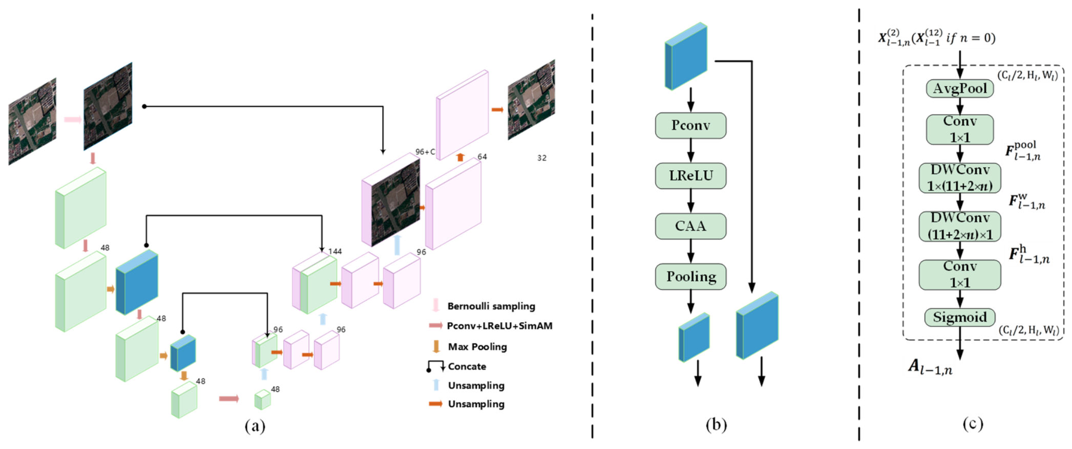
Figure 2.
CAANet overview. (a) Structure of CAANet (b) Encoder block (c) CAA module.
On the other hand, the decoder has five corresponding blocks, and the structure mirrors the encoder. The first four decoding stages start with an up-sampling step (doubling the resolution), followed by a jump connection to merge features, and finally end with two convolution layers, which are enhanced by dropout and LeakyReLU. The last step of the whole process is that three standard convolution layers- which sequentially exploit 64, 32 and C filters to reconstruct the output to the original image size H×W×C effectively.
Before starting to train the model, we should randomly sample the noisy input image Y by Bernoulli according to formula (7). This sampling process will produce two sets of results: and ,. Here b represents a single Bernoulli sample, and its probability value is between 0 and 1
The two generated images capture major contents of image Y. Hence this denoising algorithm is enhanced by optimizing the loss function in Formula (8). After stabilizing the denoising model, the trained denoiser is deployed to predict noise-mitigated image. Specifically, the noisy image will be repeatedly sampled by Bernoulli to produce several noisy images. Then, the CAANet utilizes the trained denoiser and its variants () to process noisy samples, which avoids the problem of over-fitting. Finally, the optimized images () are averaged to yield the final noise-relieved image.
In this setting, the letter M represents the total number of training epochs. Meanwhile, is the abbreviation of the denoiser. As for each , it represents the standard deviation of the corresponding . Specifically, the loss of image pair) is predominantly affected by the individual pixel values of the sampled image. Because is randomly selected, the sufficient iterations and the averaged total loss of all image pairs will guarantee the pixel differences accurately measured.
Here, represents the nth noisy image sample from a Bernoulli process.
2.3. CSBN-CVAPS Fundamentals
2.3.1. CSBN Method
Figure 3 shows the four-layer architecture of CSBN: pixel , adjacent pixel pairs (, ), bi-signal classes and land type .
According to the CSBN framework, , quantifying the likelihood that represents ground cover type , is computed as:
According to Bayesian theory, is formulated as:
Given that is the likelihood of the specific ground cover type , assuming it follows a uniform probability distribution, the conditional probability reflects the significance of the pixel pair in influencing the probability of given pixel . If all pixels within the designated neighborhood are deemed equally relevant, then simplifies to 1 divided by the number of pixels in , denoted as . The random connection between the pixel pair and the bi-signal class , which is , can be calculated accordingly:
The probabilities for the pixel , of classifying into signal classes m or n, are represented as and . These probabilities can be roughly gauged through the fuzzy membership, denoted as and , which measured by FCM_CAANet.
In the context of conditional probabilities, denotes the likelihood of a bi-signal class when given the land cover class , obtained from manually collected training samples . To compute , the bi-signal-class frequency of the land cover have to be calculated as follows:
As a soft clustering approach, FCM_CAANet ensures that both and are within the range of 0 to 1. The notation indicates the frequency of bi-signal-class for the ground cover across all bi-signal classes , where ϑ and μ ranging from 1 to . Consequently, the conditional probabilities are estimated through the following approximations:
Moreover, is computed using the law of total probability:
2.3.2. CVAPS Method
CVAPS is based on the posterior probabilities and of the pixel belonging to different ground cover types at times t1 and t2 in bitemporal remote sensing images, where and . The represents the change vector in the posterior probability space, computed as:
Change magnitude of in the posterior probability space is calculated as:
The CM map was obtained using Eq. (9). Because the posterior probabilities of the different ground cover types are between [0 1]. The magnitudes of diverse change types are scaled into the same range [0 ].
3. Datasets and Experimental Settings
Section 3.1 outlines the datasets that were employed to gauge the effectiveness of the FCC_CAANet model versus competitive methods. In Section 3.2, a more comprehensive overview of these comparative methods is offered. Finally, Section 3.3 delves into the specifics of our assessment metrics and the setting of our experiments.
3.1. Overview of Dataset
(1) For the Shangtang-1 and Shangtang-2 dataset, The RS imagery data used in Dataset Shangtang-1 and Shangtang-2 were sourced from the SenseEarth dataset provided in the 2020 World Artificial Intelligence Remote Sensing Competition organized by SenseTime [24]. The preprocess procedure includes radiation correction, geometric correction and image registration. Four ground cover types are contained in the research area: buildings, water bodies, forest land and barren land. In Dataset Shangtang-1, the biggest changes are buildings, forest land and barren areas; In Dataset Shangtang-2, forest land and barren areas are primary change regions.
(2) The DSIFN-CD dataset is obtained from Google Earth, which contains six pairs of RS images of major cities in China at different times, namely Beijing, Chengdu, Shenzhen, Chongqing, Wuhan and Xi’an [25]. We crop smaller blocks of 512×512 pixels from six pairs of images, and the spatial resolution of these blocks is 2 m/pixel. Image enhancement algorithm is applied to the RS images to improve the quality. The research area contains five different ground types-Roads, Farmland, Buildings, Wasteland, and Grassland-with the most obvious changes, mainly in barren and vegetated zones.
(3) The Lanzhou dataset is obtained from Lanzhou New District, Lanzhou, China and contains two Landsat 8 RS images, taken in 2016 and 2017 respectively [26]. These multispectral images have seven bands, the spatial resolution is 30 m/pixel, and the size is 650×650 pixels. The RS images cover various ground cover types, i.e., Forest, Farmland, Wasteland, Mountains, and Buildings.
(4) The Guangzhou dataset is obtained from the CD_Data_GZ archive [27], is utilized to evaluate the proposed method on very-high-resolution remote sensing imagery exhibiting substantial spectral variation. This dataset (DS5) comprises two RGB images with a spatial resolution of 0.55 m and dimensions of 1708 × 1708 pixels, and the two acquisition times display marked spectral differences.
3.2. Comparative Approaches
In our experiments, two conventional algorithms and three unsupervised deep learning algorithms are selected to verify the superiority of the proposed method. Traditional methods are INLPG [28], and ASEA [29]. INLPG improves graph construction, structural difference calculation and difference image fusion in the nonlocal patch graph method, so it can achieve good change detection ability under noise interference. ASEA incorporates spatial context information from very high-resolution remote sensing images. It introduces a band-to-band distance metric to measure changes between multi-temporal images within a dynamically adjusted spatial context. Studies have shown that this approach reduces noise interference and improves detection accuracy.
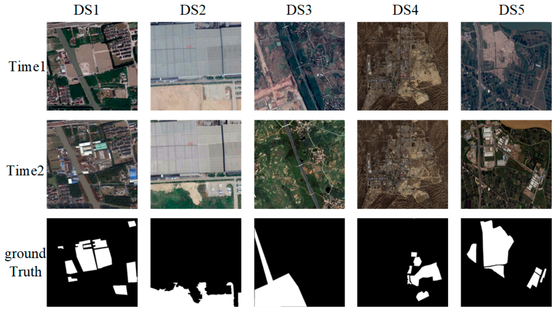
Figure 4.
Dataset and ground truth images.
The selected unsupervised deep learning CD methods include GMCD [30], KPCAMNet [31] and DCVA [32]. GMCD improves the reliability of change detection by introducing noise modeling directly into the feature learning structure of full convolution network to suppress noise interference. KPCAMNet uses kernel principal component analysis convolution to obtain complex spectral and spatial feature representation, then projects the feature changes into polar coordinate system, and finally generates detection results through threshold segmentation and clustering technology. DCVA uses pre-trained convolutional neural network to extract the spatial context and accurately identify the changed pixels.
3.3. Experimental Setup and Assessment Criteria
All the experiments are executed on NVIDIA RTX 4080 GPU, Intel i9-13900K 3.0 GHz CPU, and 64GB RAM.
The parameters of each comparative method are set as follows: DCVA uses layers {2, 5, 8}; KPCAMNet uses a four-layer network with eight KPCA convolution kernels of radial basis functions. GMCD has been trained for 40 epochs. All methods use the default parameters specified in the original papers and follow the same post-processing steps for objective comparison. To test anti-noise performance, Gaussian noise (mean 0.00 and variance 0.05) is added to the target remote sensing images.
The performance metrics include miss alarm (MA), false alarm (FA), precision, recall, F1 score, overall accuracy (OA), and Kappa coefficient. These metrics are derived from: MA = FN/(TP+FN), FA = FP/(FP+TN), precision = TP/(TP+FP), recall = TP/(TP+FN), OA = (TP+TN)/(TP+TN+FP+FN), F1 = (2×precision×recall)/(precision+recall), and Kappa = (OA-Pe)/(1-Pe), where Pe = [(TP+FP)(TP+FN)+(FN+TN)(FP+TN)]/(TP+TN+FP+FN)^2. Here, FN refers to pixels mistakenly determined to be unchanged, and FP refers to pixels mistakenly labeled as changed. TN denotes the pixels that are correctly recognized as unchanged, whereas TP represents those accurately classified as changed. Kappa is a comprehensive CD performance measurement.
4. Experimental Results
4.1. Comparison with State-of-the-Art Methods Under Gaussian Noise
In this experiment, mean 0 and variance 0.05 Gaussian noise is applied to contaminate RS imagery. The proposed FCM_CAANet divides image into 30 signal classes with fuzzy parameter 3.5. The Otsu algorithm [33] is utilized to generate CD maps, where the FA and MD areas are marked in red and green respectively.
As shown in Figure 5, the CD performance of proposed method on Shangtang-1 and Shangtang-2 obviously outperforms other comparative methods. Moreover, under Gaussian noises, the proposed method also maintains superior performance. According to Table 1, FCC_CAANet obtained the highest OA of 0.9280 and Kappa coefficient of 0.8134 on Shangtang-1, and achieved an OA of 0.9633 and a Kappa coefficient of 0.9521 on Shangtang-2. The Shangtang-1 dataset has wasteland, buildings, farmland and grassland, where changes mainly occur in wasteland and forest areas, causing many FAs in competitive methods. For example, KPCAMNet, GMCD, and DCVA mistakenly mark a large area of vegetation as changing areas. In particular, KPCAMNet also miss some real changes. In comparison, the proposed approach can suppress such erroneous responses and produce change-detection outputs that are both distinct and trustworthy.
In the area of Shangtang-2 (Figure 6), the main changes are buildings, grasslands and wasteland, which are dominated by grassland. Except KPCAMNet, INPGL and DCVA, which are seriously disturbed by noise, other competitive algorithms can still detect the major changing areas. However, it should be noticed that our method accomplished the best CD performance. As evidenced in Table 1, FCC_CAANet obtained the lowest missed alarm rate (0.1417) and the highest OA and Kappa values. Although FCM_SICM and other competitors can detect most of the change areas, they still miss some major changing areas under noise interference.
FCC_CAANet performs particularly well on Dataset Shangtang-1 and SenseTime Shangtang-2. Both data sets are 512×512 in size, and the spatial resolution is 1-3 meters. These results confirm that our method has superior CD performance on small-scale high-resolution RS imagery. This improvement primarily stems from combining contextual cues with spatial–intensity features, together with employing membership linkage mechanisms that help prevent the algorithm from converging too early.
The dataset DSIFN-CD (Figure 7) is mainly occupied by farmland and grassland, and the changes mainly occur in farmland areas. The competitive methods produce high FAs. Specifically, KPCAMNET, GMCD and DCVA are adversely affected by noise interference, mistaking many vegetation areas as changed. Also, KPCAMNET has missed many real changes. Comparatively, our method only slightly suffered from FAs and MDs, and produced the clearest and accurate CD map.
Looking at LZ dataset (Figure 8), FCC_CAANet generates the best CD result. Compared with other algorithms, it committed the least mistakes. As illustrated in Figure 8, GMCD, DCVA, and PCAKMeans generated extensive false-alarm regions, whereas KPCAMNet resulted in a substantial number of missed detections. These inferior results have to be attributed to the 30 m/pixel resolution of the LZ dataset, where mixed pixel phenomena are ubiquitous; Even CAANet alone can suppress some noise interference, it cannot deal with mixed pixels within LZ dataset. FCM_CAANet, on the other hand, divides mixed pixels into different signal classes, each of which represents pixels with similar spectral characteristics, so that it can simultaneously cope with noise interference and mixed pixel problems.
The dataset Guangzhou (Figure 9) is made of high-resolution remote sensing images. It contains the largest RS images among the selected datasets, with the most diverse land types, and the most complex changing areas. In this dataset, the main changes occur in buildings and forests, which have obvious spectral changes and thus particularly require the incorporation of spatial information into the CD process. On this dataset, our method accomplished the highest OA. Specifically, Our OA and Kappa are 0.11502 and 0.00803 higher than the second-best method. Although VHR images contain few mixed pixels, they have very complex spatial details. Since the proposed method integrates spatial information through FCM_CAANet and CSBN, the yielded CD map has smooth edges and few gaps, which contributes to the superior CD performance of our method.
4.2. Sensitivity Analysis Under Different Gaussian Noise Levels
In this subsection, the sensitivity of six competitive methods to different levels of Gaussian noises are analyzed. The Gaussian noises of different levels are applied to pollute the target RS imagery, and the noise levels are 0.01, 0.03, 0.05, 0.07 and 0.09 respectively. The number of signal classes is set 10 and the fuzzy parameter q is set to 3.5. To ensure the objectivity of performance comparison, the same post-processing steps are applied for all competitors.
As shown in Figure 10, the proposed method maintains stable and superior performance under different noise levels. In all the five datasets, its Kappas fluctuated slightly with only 0.0751 magnitude. In contrast, DCVA is very sensitive to noise interference, with unsatisfied CD results obtained on all datasets. As for the ASEA method, it accomplishes good CD performance under mild noise interference. However, under severe noise contamination, its performance is inferior to our method. The Kappa trend of GMCD method is similar to that of ASEA. In medium-resolution RS images (such as Lanzhou data set), its performance deteriorates with the elevated noise level. However, in the Shangtang-1 dataset, the overall performance of GMCD has an upward trend. The reason may be attributed to the randomness of added noises. In particular, when the noise level increases, many strong noises occur in the MD holes of detected CD areas. In post-processing, morphological dilation operation will fill holes with strong noises, while other isolated noise points will be removed as small spots, which accidentally enhances the CD accuracy. This analysis can be applied to explain the upward performance of KPCAMNet under the increasing noise level on all data sets except Shangtang-2. Overall, as indicated in Figure 10, both GMCD and INLPG can resist the Gaussian noise to a certain extent. But they exhibit unsatisfactory stability and consistency which are obviously inferior to our method.

Table 2.
The performance of competitive methods on the five datasets.
| Dataset | Method | Noise level | |||||
| 0.01 | 0.03 | 0.05 | 0.07 | 0.09 | |||
| Shangtang-1 | GMCD | 0.7949 | 0.7943 | 0.7972 | 0.7893 | 0.7908 | |
| KPCAMNet | 0.3012 | 0.3355 | 0.3343 | 0.3012 | 0.3243 | ||
| DCVA | 0.0569 | 0.0275 | 0.0069 | 0.0024 | 0.0501 | ||
| ASEA | 0.3543 | 0.3579 | 0.3261 | 0.3185 | 0.3037 | ||
| INLPG | 0.6578 | 0.6273 | 0.6292 | 0.5876 | 0.0427 | ||
| Ours | 0.8476 | 0.8256 | 0.8139 | 0.8065 | 0.7921 | ||
| Shangtang-2 | GMCD | 0.9412 | 0.9412 | 0.9426 | 0.9366 | 0.9255 | |
| KPCAMNet | 0.2401 | 0.1282 | 0.1151 | 0.1168 | 0.1305 | ||
| DCVA | 0.1213 | 0.0225 | 0.0024 | 0.0462 | 0.0368 | ||
| ASEA | 0.8188 | 0.8196 | 0.8190 | 0.8172 | 0.8090 | ||
| INLPG | 0.2650 | 0.4149 | 0.4306 | 0.4217 | 0.4124 | ||
| Ours | 0.9503 | 0.9429 | 0.9521 | 0.9423 | 0.9417 | ||
| GMCD | 0.7488 | 0.7231 | 0.7325 | 0.7544 | 0.7392 | ||
| DSIFN-CD | KPCAMNet | 0.1868 | 0.2360 | 0.2413 | 0.2395 | 0.2621 | |
| DCVA | 0.0534 | 0.0326 | 0.0017 | 0.0184 | 0.0089 | ||
| ASEA | 0.5715 | 0.5660 | 0.5560 | 0.5312 | 0.5123 | ||
| INLPG | 0.3504 | 0.5784 | 0.4635 | 0.6398 | 0.6984 | ||
| Ours | 0.8701 | 0.8768 | 0.8855 | 0.8878 | 0.8769 | ||
| GMCD | 0.5104 | 0.5171 | 0.3190 | 0.2226 | 0.1837 | ||
| Lanzhou | KPCAMNet | 0.4867 | 0.4967 | 0.4894 | 0.4771 | 0.4513 | |
| DCVA | 0.0846 | 0.0566 | 0.0497 | 0.0287 | 0.0365 | ||
| ASEA | 0.4961 | 0.4538 | 0.3967 | 0.3452 | 0.2887 | ||
| INLPG | 0.6957 | 0.6730 | 0.6530 | 0.6556 | 0.6946 | ||
| Ours | 0.7406 | 0.7549 | 0.7296 | 0.7550 | 0.7257 | ||
| Guangzhou | GMCD | 0.5978 | 0.7392 | 0.7714 | 0.7317 | 0.7367 | |
| KPCAMNet | 0.3522 | 0.4778 | 0.5053 | 0.5123 | 0.5103 | ||
| DCVA | 0.1827 | 0.0492 | 0.0470 | 0.0747 | 0.0810 | ||
| ASEA | 0.4015 | 0.3906 | 0.3906 | 0.3411 | 0.3223 | ||
| INLPG | 0.7820 | 0.7714 | 0.7125 | 0.7292 | 0.7140 | ||
| Ours | 0.8233 | 0.8021 | 0.7794 | 0.7637 | 0.7482 | ||
4.3. Ablation Study
The contaminated Shangtang-1 dataset (0.05 Gaussian noise) is used for the performance analysis of each module in FCC_CAANet. A total of ten models (from A1 to A10) are implemented to test the corresponding modules of the proposed framework. In this experiment, models A1 to A9 all contain both a denoising network and a change detection module, whereas A10 contains only the change detection module without the denoising module. The number of signal classes is set to 10, fuzzy parameter is set to 3.5, and the number of training samples is set to 3000. The same post-processing procedures are applied for each individual model.
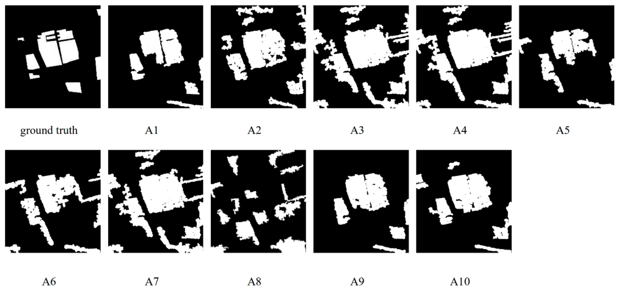
Figure 11.
Change maps obtained by ten ablation variants on the Shangtang-1 dataset.
As shown in Table 3, we observe that the Kappa values of A9, which replaces CAANet with Self2Self, and A10, which performs change detection directly after completely removing the denoising module, decreased by 0.0667 and 0.0867, respectively, compared with A1, indicating that the denoising network plays a role in improving change detection accuracy. Although A3–A6 constitute fully implemented two-stage frameworks for change detection, they only incorporate local spatial information and exhibit weak robustness to Gaussian noise, resulting in unsatisfactory detection accuracy. The best and worst Kappa accuracies of these models deviate from those of A1 by 0.33331 and 0.06673, respectively. This discrepancy arises because spatial FCM relies solely on neighborhood information, causing the resulting signal-class centers to be heavily contaminated by stochastic noise. Moreover, if the signal centers identified by fuzzy clustering algorithms are significantly corrupted by noise, subsequent CSBN and CVAPS will incur substantial computational errors and yield unsatisfactory CD results. A2 obtains the second-best Kappa value among all ablation variants, falling short of A1 by only 0.0339. This is because it not only uses a distance metric that integrates spatial and spectral information but also adopts an adaptive cluster center initialization strategy that dynamically adjusts the initial cluster centers based on local pixel information, enabling them to more accurately represent each class and thereby improving clustering robustness. Notably, A10 achieves the third-highest Kappa after A1 and A2 (0.7522), indicating that the change detection stage of the proposed framework is also robust to noise.
4.4. Parameter Sensitivity Analysis
4.4.1. Fuzziness q
In this subsection, experiments are conducted on five datasets to analyze the effect of fuzziness q on FCC_CAANet. These data sets are polluted by Gaussian noise with a mean of 0 and a variance of 0.05. The seven q values (1.5, 2.0, 2.5, 3.0, 3.5, 4.0,4.5) are set to test their effect on the Kappa coefficient of the proposed method, which are detailed in Figure 12 and Table 4.
In the medium- to high-resolution RS imagery from Shangtang-1, Shangtang-2, and DSIFN-CD, when fuzziness q drops below 3.0, the Kappa values of FCC_CAANet are generally lower. Moreover, in high-resolution RS images from Lanzhou and Guangzhou datasets, the Kappa of FCC_CAANet exhibits an noticeable decrease, especially when the fuzziness q is limited to 1.5 and lower. This decline is due to insufficient mixed pixel decomposition of FCM_CAANet when the fuzziness is low. Moreover, the reduction of fuzziness contributes to an elevated cumulative clustering error, lowers the uncertainty in mixed pixel decomposition, and consequently reduces the uncertainty of the probability vector estimated by CSBN, thereby boosting the FA rate. Similarly, when the q value exceeds 3.5, the Kappa significantly declines. This is due to the high fuzziness, which may also reduce the accuracy of mixed pixel decomposition, increase the uncertainty of the estimated posterior probability vectors and MD rates, and thus lower the Kappa value. Therefore, it is necessary to select proper fuzziness q through experiment. In this paper, the optimal fuzziness value is dataset-dependent: most datasets achieve their best Kappa when q = 3.0, while the Lanzhou dataset obtains its highest Kappa at q = 3.5.
4.4.2. Win Size
As evidenced in Figure 13, the window size has a considerable effect on CD performance.
According to experimental results of Shangtang-1, Shangtang-2, and DSIFN-CD, it is observed that the RS images with less complicated spatial features require a small window size to achieve satisfactory performance. However, a too small window size cannot sufficiently suppress the noise in the target images, resulting in poor detection results. In contrast, for RS imagery with a complex spatial structure, the window size needs to be enlarged to obtain the optimal Kappa, as indicated in the experimental results on the Lanzhou and Guangzhou datasets. Therefore, it is necessary to choose different optimal window sizes for remote sensing images with different spatial complexity. In summary, when the spatial distribution of ground structure in an RS image is more complex, a larger window size is preferred to sufficiently capture the spatial details and generate satisfactory CD results.
Table 5.
CD performance of win size on algorithm results.
| Dataset | Win size | |||||||
| 5 | 6 | 7 | 8 | 9 | 10 | 11 | 12 | |
| Shangtang-1 | 0.7800 | 0.7871 | 0.7924 | 0.8002 | 0.8139 | 0.8108 | 0.8001 | 0.7913 |
| Shangtang-2 | 0.8490 | 0.8912 | 0.9052 | 0.9245 | 0.9521 | 0.9515 | 0.9238 | 0.9012 |
| DSIFN-CD | 0.8373 | 0.8522 | 0.8722 | 0.8854 | 0.8855 | 0.8756 | 0.8746 | 0.8665 |
| Lanzhou | 0.6753 | 0.6848 | 0.6975 | 0.7066 | 0.7165 | 0.7245 | 0.7281 | 0.7296 |
| Guangzhou | 0.6845 | 0.6971 | 0.7314 | 0.7463 | 0.7614 | 0.7732 | 0.7742 | 0.7794 |
4.5. Algorithm Running Time
As observed in Table 6, KPCAMNet completes the CD task in 5.46 seconds at the cost of CD accuracy, making it the fastest among the seven competitors. On the other hand, GMCD and DCVA complete the CD task in 10.29s and 10.78s, respectively, due to the exploitation of the pre-trained parameters. In contrast, the ASEA algorithm is slower due to adaptive spatial feature extraction and continuous expansion of the contextual neighborhood. Without the denoising network CAANet, the FCC method consumes 155.66 seconds due to the incorporation of spatial information by CSBN, which requires a significant amount of processing time. In contrast, FCC_CAANet takes the longest running time due to its denoising network, which consumes a significant amount of computational resources to denoise the contaminated RS images. Specifically, CAANet consumes 1108.10 seconds to complete 15,000 iterations, which occupies a substantial portion of the total processing time. However, by adjusting the number of processing iterations, the proposed method can balance the required time and anti-noise performance according to various application scenarios.
5. Conclusions
In our research, we introduce a novel anti-noise RS CD framework, referred to as FCC_CAANet. The proposed framework exploits CAANet to restore the RS images from Gaussian noise pollution and counteract noise interference on the accuracy of RS CD. Moreover, the fuzzy clustering module of the proposed framework (FCM_CAANet) can distinguish the spatial and spectral details from the restored image. By using membership linkage in the clustering process, the FCM_CAANet can accurately divide pixels into different signal classes by effective noise filtration. To further suppress Gaussian noise, the CSBN is employed to estimate the posterior probability vector at the pixel level in a spatially sensitive manner and to generate an accurate change map under noise interference. Experimental results on five public datasets verify that the proposed FCC_CAANet outperforms current CD competitors under Gaussian noise interference, yielding clearer change areas and sharper edges. To further reduce the high computational load, we plan to develop parallelized FCM_CAANet and CSBN in our future work.
Author Contributions
Conceptualization, R.Z. and J.S.; methodology, R.Z. and J.S.; software, J.S.; validation, Y.L., Y.H. and X.L.; formal analysis, Y.L. and Y.H.; investigation, R.Z.; data curation, Y.L. and Y.H.; writing—original draft preparation, R.Z.; writing—review and editing, R.Z., J.S., Y.L., Y.H., S.Y. and X.L.; visualization, S.Y. and X.L.; supervision, J.S.; project administration, J.S.; funding acquisition, J.S. All authors have read and agreed to the published version of the manuscript.
Funding
This research was funded by the Gansu Provincial Education Science and Technology Innovation Project (Grant No. 2026CXZX-628), the National Key R&D Program of China (Grant No. 2022YFA3903604), and the Gansu Province Basic Innovation Group Project (Grant No. 24JRRA220).
Data Availability Statement
The public datasets used in this study are available from the sources cited in the manuscript. The processed data and code are available from the corresponding author upon reasonable request.
Acknowledgments
The authors are grateful to the editor and anonymous reviewers for their helpful and valuable suggestions.
Conflicts of Interest
The authors declare no conflicts of interest.
References
- Li, X.; Yan, H.; Xie, W.; Kang, L.; Tian, Y. An improved pulse-coupled neural network model for pansharpening. Sensors 2020, 20, 2764–2783. [Google Scholar] [CrossRef] [PubMed]
- Qin, H.; Wang, J.; Mao, X.; Zhao, Z.; Gao, X.; Lu, W. An improved Faster R-CNN method for landslide detection in remote sensing images. J. Geovisualization Spat. Anal. 2023, 8, 2. [Google Scholar] [CrossRef]
- Xu, X.; Li, X.; Li, Y.; Kang, L.; Ge, J. A novel adaptively optimized PCNN model for hyperspectral image sharpening. Remote Sens. 2023, 15, 4205. [Google Scholar] [CrossRef]
- Chen, D.; Kang, J.; Wang, L.; et al. SACNet: A novel self-supervised learning method for shadow detection from high-resolution remote sensing images. J. Geovisualization Spat. Anal. 2025, 9(1), 14. [Google Scholar] [CrossRef]
- Wu, T.; Sha, T.; Yao, X.; et al. Improvement of the YOLO series for detecting tower cranes based on high-resolution remote sensing imagery. J. Geovisualization Spat. Anal. 2025, 9(1), 8. [Google Scholar]
- Guangwei, Sheng. Forest Land Change Detection Based on Angle Priority Change Vector Analysis [D]; Nanjing University, 2020. [Google Scholar]
- Li, L.; Li, X.; Zhang, Y.; Wang, L.; Ying, G.; et al. Change detection for high-resolution remote sensing imagery using object-oriented change vector analysis method. In IGARSS 2016 – IEEE International Geoscience and Remote Sensing Symposium; 2016, pp. 2873–2876.
- Chen, J.; Chen, X.; Cui, X.; et al. Change vector analysis in posterior probability space: A new method for land cover change detection. IEEE Geosci. Remote Sens. Lett. 2011, 8(2), 317–321. [Google Scholar] [CrossRef]
- Li, Y.; Li, X.; Song, J.; Wang, Z.; He, Y.; Yang, S. Remote-sensing-based change detection using change vector analysis in posterior probability space: A context-sensitive Bayesian network approach. IEEE J. Sel. Top. Appl. Earth Obs. Remote Sens. 2023, 16, 3198–3217. [Google Scholar] [CrossRef]
- Li, Yikun; Yang, Yang; Yang, Shuwen; et al. Posterior Probability Spatial Change Vector Analysis of Remote Sensing Images Coupling Fuzzy C-Means Clustering and Bayesian Network. J. Remote Sens. Nat. Resour. 2021, 33(4), 82–88. [Google Scholar]
- Chen, P.; Li, C.; Zhang, B.; Chen, Z.; Yang, X.; Lu, K.; Zhuang, L. A region-based feature fusion network for VHR image change detection. Remote Sens. 2022, 14, 5577. [Google Scholar] [CrossRef]
- Wang, J.; Zhao, T.; Jiang, X.; Lan, K. A hierarchical heterogeneous graph for unsupervised SAR image change detection. IEEE Geosci. Remote Sens. Lett. 2022, 19, 4516605. [Google Scholar] [CrossRef]
- Zhao, H.; Liu, S.; Du, Q.; Bruzzone, L.; Zheng, Y.; Du, K.; Tong, X.; Xie, H.; Ma, X. GCFnet: Global collaborative fusion network for multispectral and panchromatic image classification. IEEE Trans. Geosci. Remote Sens. 2022, 60, 5632814. [Google Scholar] [CrossRef]
- Zhang, H.; Yao, J.; Ni, L.; Gao, L.; Huang, M. Multimodal attention-aware convolutional neural networks for classification of hyperspectral and LiDAR data. IEEE J. Sel. Top. Appl. Earth Obs. Remote Sens. 2023, 16, 3635–3644. [Google Scholar] [CrossRef]
- Zhang, K.; Zuo, W.; Chen, Y.; Meng, D.; Zhang, L. Beyond a Gaussian denoiser: Residual learning of deep CNN for image denoising. IEEE Trans. Image Process. 2017, 26, 3142–3155. [Google Scholar] [CrossRef] [PubMed]
- Jing, W.C.; Hong, Y.C.; Ming, Y. Image blind denoising with generative adversarial network based noise modeling. In Proceedings of the IEEE Conference on Computer Vision and Pattern Recognition, 2018; pp. 3155–3164. [Google Scholar]
- Valsesia, D.; Fracastoro, G.; Magli, E. Deep graph-convolutional image denoising. IEEE Trans. Image Process. 2020, 29, 8226–8237. [Google Scholar] [CrossRef]
- Ma, Y.; Liu, X.R.; Zhao, T.; Liu, Y.; Tang, J.; Shah, N. A unified view on graph neural networks as graph signal denoising. In Proceedings of the 30th ACM International Conference on Information and Knowledge Management, 2021; pp. 1202–1211. [Google Scholar]
- Rey, S.; Segarra, S.; Heckel, R.; Marques, A.G. Untrained graph neural networks for denoising. IEEE Trans. Signal Process. 2022, 70, 5708–5723. [Google Scholar] [CrossRef]
- Wang, Q.; Wang, X.; Fang, C.; Yang, W. Robust fuzzy C-means clustering algorithm with adaptive spatial & intensity constraint and membership linking for noise image segmentation. Appl. Soft Comput. 2020, 92, 106318. [Google Scholar] [CrossRef]
- Ahmed, M.N.; Yamany, S.M.; Mohamed, N.; Farag, A.A.; Moriarty, T. A modified fuzzy C-means algorithm for bias field estimation and segmentation of MRI data. IEEE Trans. Med. Imaging 2002, 3, 193–199. [Google Scholar] [CrossRef]
- Chaudhury, K.N.; Dabhade, S.D. Fast and provably accurate bilateral filtering. IEEE Trans. Image Process. 2016, 25, 2519–2528. [Google Scholar] [CrossRef] [PubMed]
- Cai, X.; Lai, Q.; Wang, Y.; Wang, W.; Sun, Z.; Yao, Y. Poly Kernel Inception Network for remote sensing detection. arXiv 2024, arXiv:2403.06258. [Google Scholar]
- SenseEarth. Available online: https://rs.sensetime.com/.
- Zhang, C.; Yue, P.; Tapete, D.; Jiang, L.; Shangguan, B.; Huang, L.; Liu, G. A deeply supervised image fusion network for change detection in high-resolution bi-temporal remote sensing images. ISPRS J. Photogram. Remote Sens. 2020, 166, 183–200. [Google Scholar] [CrossRef]
- Geospatial Data Cloud. Available online: https://www.gscloud.cn/sources/ (accessed on 5 June 2022).
- Peng, D.; Bruzzone, L.; Zhang, Y.; Guan, H.; Ding, H.; Huang, X. SemiCDNet: A semisupervised CNN for change detection in high-resolution remote-sensing images. IEEE Trans. Geosci. Remote Sens. 2021, 59, 5891–5906. [Google Scholar] [CrossRef]
- Sun, Y.; Lei, L.; Li, X.; Tan, X.; Kuang, G. Structure consistency-based graph for unsupervised change detection with homogeneous and heterogeneous remote sensing images. IEEE Trans. Geosci. Remote Sens. 2022, 60, 4700221. [Google Scholar] [CrossRef]
- Lv, Z.; Wang, F.; Liu, T.; Kong, X.; Benediktsson, J.A. Novel automatic approach for land cover change detection by using VHR remote sensing images. IEEE Geosci. Remote Sens. Lett. 2021, 19, 8016805. [Google Scholar] [CrossRef]
- Tang, X.; Zhang, H.; Mou, L.; Liu, F.; Zhang, X.; Zhu, X.; Jiao, L. An unsupervised remote sensing change detection method based on multiscale graph convolutional network and metric learning. IEEE Trans. Geosci. Remote Sens. 2022, 60, 5632814. [Google Scholar] [CrossRef]
- Wu, C.; Chen, H.; Du, B.; Zhang, L. Unsupervised change detection in multitemporal VHR images based on deep kernel PCA convolutional mapping network. IEEE Trans. Cybern. 2022, 52, 12084–12098. [Google Scholar] [CrossRef] [PubMed]
- Saha, S.; Bovolo, F.; Bruzzone, L. Unsupervised deep change vector analysis for multiple-change detection in VHR images. IEEE Trans. Geosci. Remote Sens. 2019, 57, 3677–3693. [Google Scholar] [CrossRef]
- Lv, Z.Y.; Liu, T.; Zhang, P.; Benediktsson, J.A.; Lei, T.; Zhang, X. Novel adaptive histogram trend similarity approach for land cover change detection using bitemporal VHR images. IEEE Trans. Geosci. Remote Sens. 2019, 57, 9554–9574. [Google Scholar] [CrossRef]
- Krinidis, S.; Chatzis, V. A robust fuzzy local information C-means clustering algorithm. IEEE Trans. Image Process. 2010, 19, 1328–1337. [Google Scholar] [CrossRef] [PubMed]
- Chen, S.; Zhang, D. Robust image segmentation using FCM with spatial constraints based on new kernel-induced distance measure. IEEE Trans. Syst. Man. Cybern. B 2004, 34, 1907–1916. [Google Scholar] [CrossRef]
- Tong, S.; Li, S. Design of VGG structured U-Net model for remote sensing green space information extraction. J. Geovisualization Spat. Anal. 2025, 9(1), 5. [Google Scholar]
Figure 1.
Flowchart of the proposed FCC_CAANet framework.
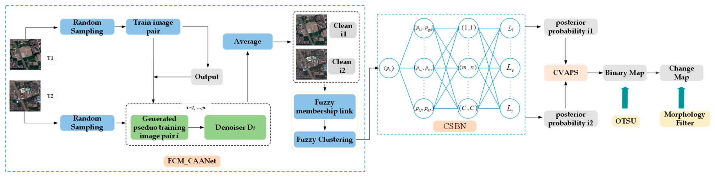
Figure 3.
Context-Sensitive Bayesian Network.
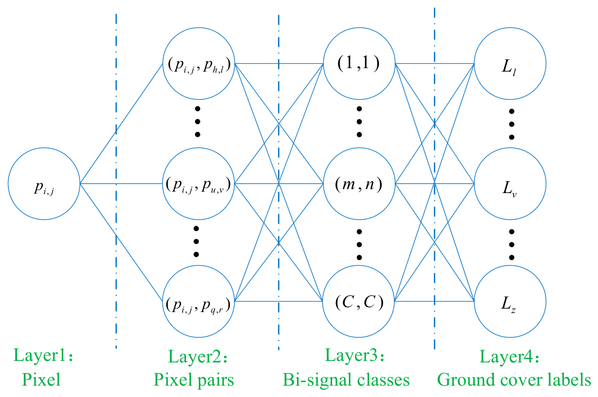
Figure 5.
CD results of competitive methods obtained on Shangtang-1. (a) Time 1 image with Gaussian noises. (b) Time 2 image with Gaussian noises. (c) Ours. (d) DCVA. (e). KPCAMNet (f). GMCD (g). INLPG (h). ASEA (i). Ground truth.
Figure 5.
CD results of competitive methods obtained on Shangtang-1. (a) Time 1 image with Gaussian noises. (b) Time 2 image with Gaussian noises. (c) Ours. (d) DCVA. (e). KPCAMNet (f). GMCD (g). INLPG (h). ASEA (i). Ground truth.
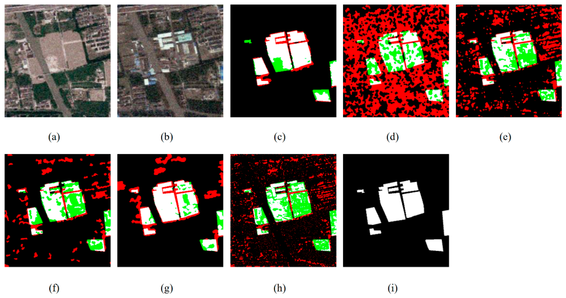
Figure 6.
CD results of competitive methods obtained on Shangtang-2. (a) Time 1 image with Gaussian noises. (b) Time 2 image with Gaussian noises. (c) Ours. (d) DCVA. (e). KPCAMNet (f). GMCD (g). INLPG (h). ASEA (i). Ground truth.
Figure 6.
CD results of competitive methods obtained on Shangtang-2. (a) Time 1 image with Gaussian noises. (b) Time 2 image with Gaussian noises. (c) Ours. (d) DCVA. (e). KPCAMNet (f). GMCD (g). INLPG (h). ASEA (i). Ground truth.
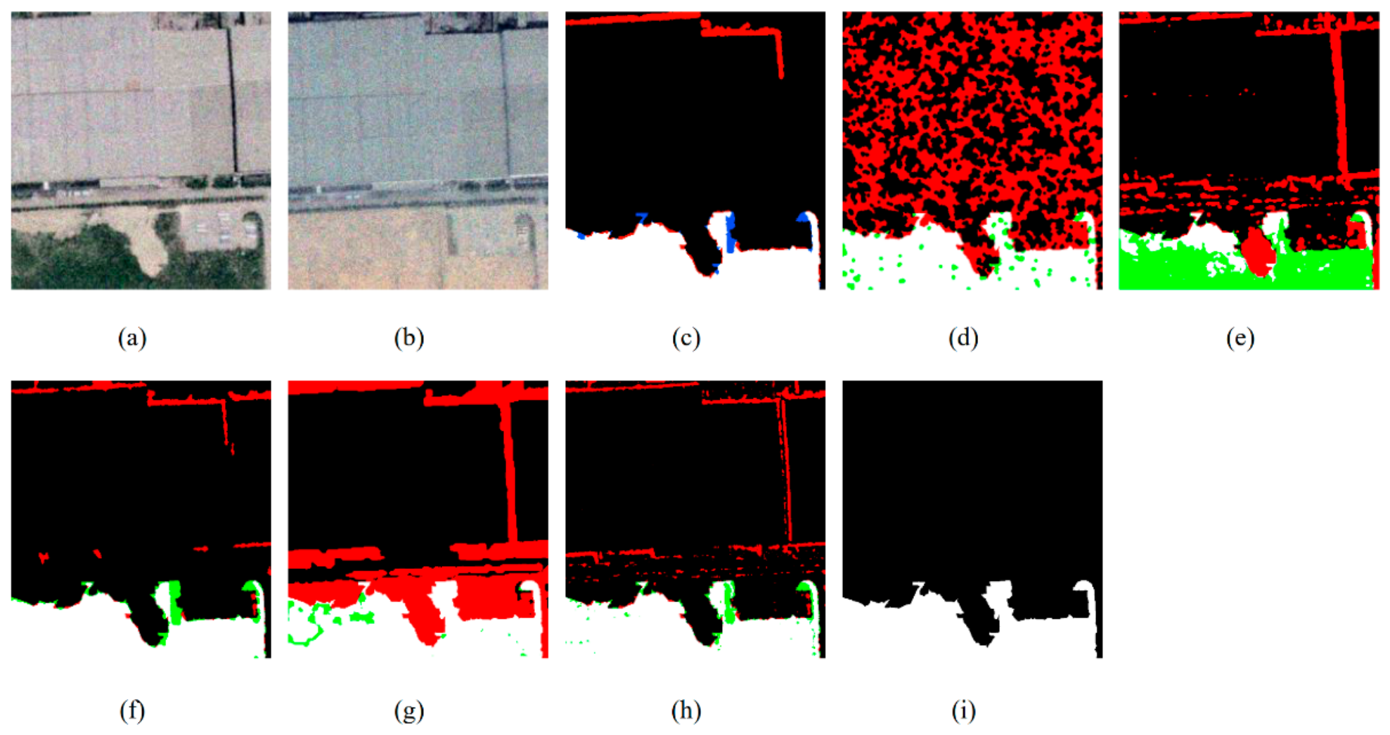
Figure 7.
CD results of competitive methods obtained on DSIFN-CD. (a) Time 1 image with Gaussian noises. (b) Time 2 image with Gaussian noises. (c) Ours. (d) DCVA. (e). KPCAMNet (f). GMCD (g). INLPG (h). ASEA (i). Ground truth.
Figure 7.
CD results of competitive methods obtained on DSIFN-CD. (a) Time 1 image with Gaussian noises. (b) Time 2 image with Gaussian noises. (c) Ours. (d) DCVA. (e). KPCAMNet (f). GMCD (g). INLPG (h). ASEA (i). Ground truth.
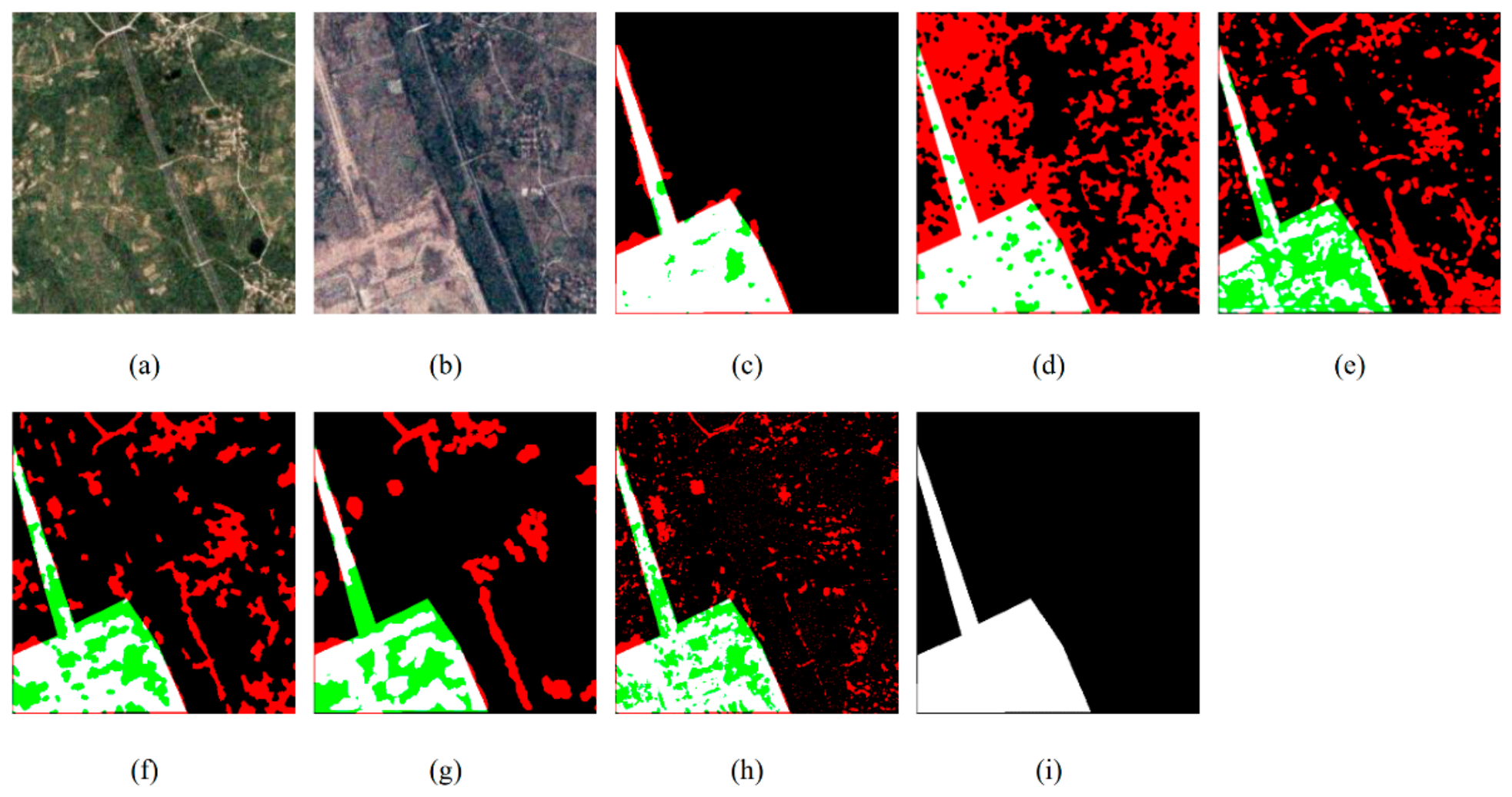
Figure 8.
CD results of competitive methods obtained on Lanzhou. (a) Time 1 image with Gaussian noises. (b) Time 2 image with Gaussian noises. (c) Ours. (d) DCVA. (e). KPCAMNet (f). GMCD (g). INLPG (h). ASEA (i). Ground truth.
Figure 8.
CD results of competitive methods obtained on Lanzhou. (a) Time 1 image with Gaussian noises. (b) Time 2 image with Gaussian noises. (c) Ours. (d) DCVA. (e). KPCAMNet (f). GMCD (g). INLPG (h). ASEA (i). Ground truth.
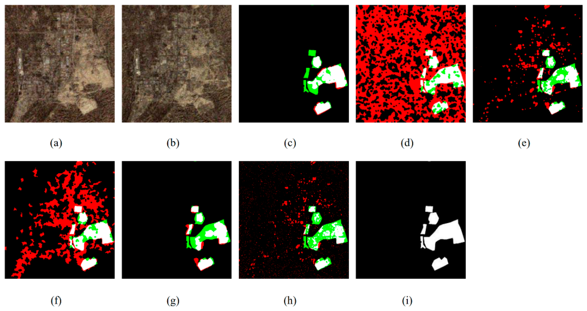
Figure 9.
CD results of competitive methods obtained on Guangzhou. (a) Time 1 image with Gaussian noises. (b) Time 2 image with Gaussian noises. (c) Ours. (d) DCVA. (e). KPCAMNet (f). GMCD (g). INLPG (h). ASEA (i). Ground truth.
Figure 9.
CD results of competitive methods obtained on Guangzhou. (a) Time 1 image with Gaussian noises. (b) Time 2 image with Gaussian noises. (c) Ours. (d) DCVA. (e). KPCAMNet (f). GMCD (g). INLPG (h). ASEA (i). Ground truth.
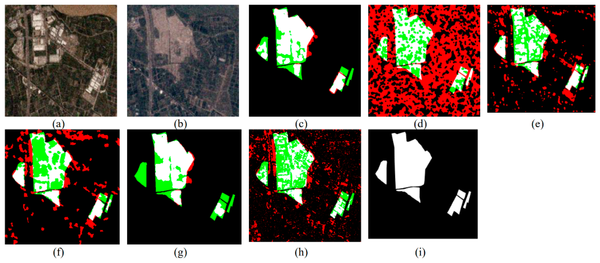
Figure 10.
Noise-resistance performance of competitive methods on the five datasets.
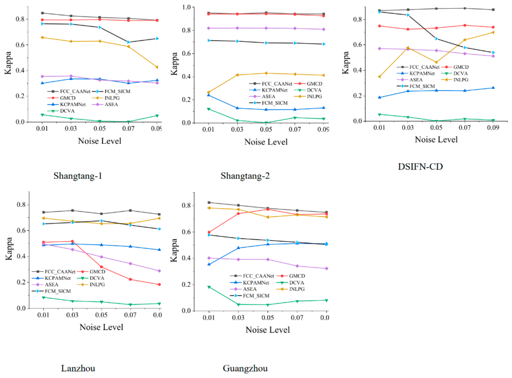
Figure 12.
Effect of fuzzy degree m on algorithm results.
Figure 13.
Effect of win size on algorithm results.
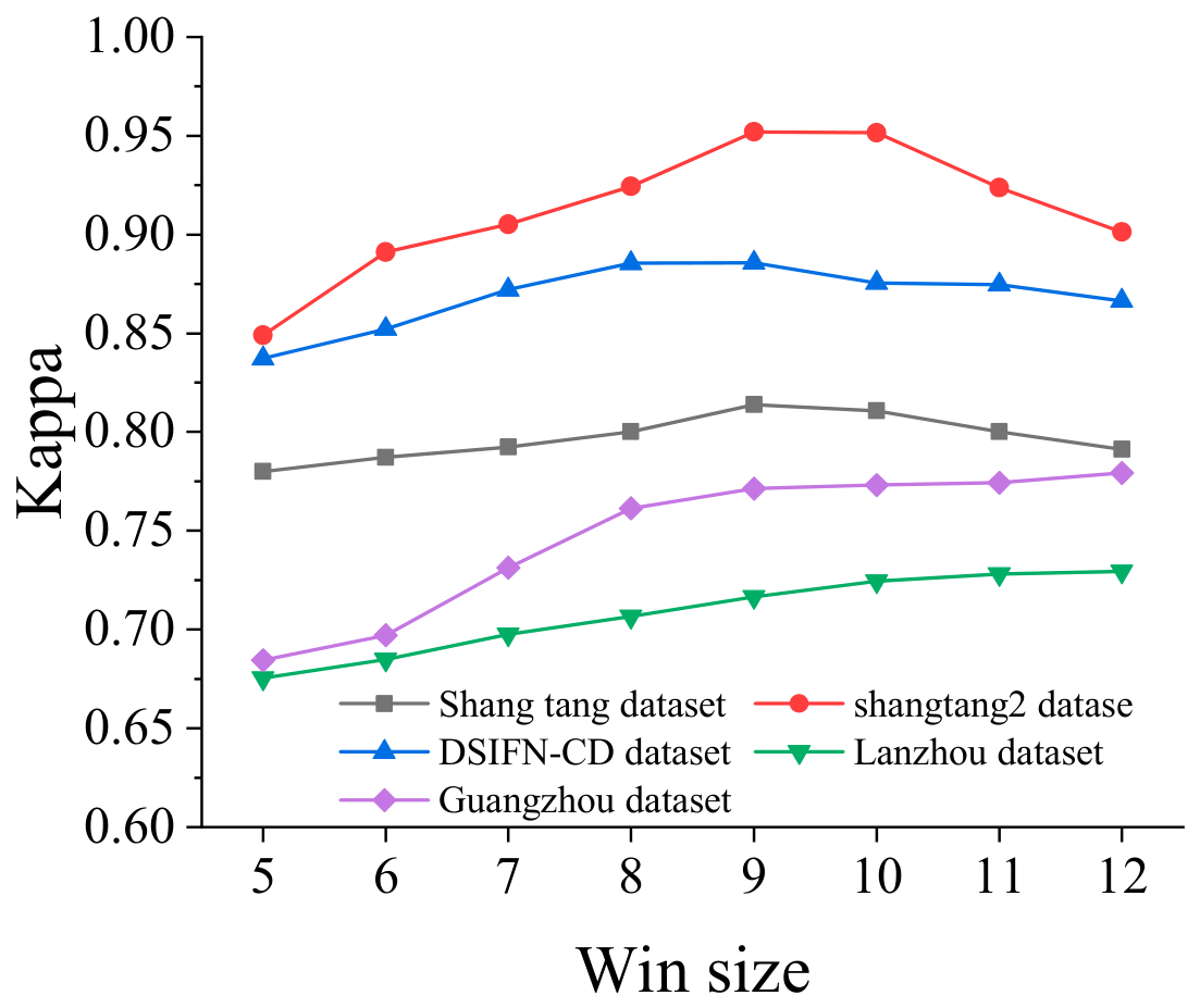
Table 1.
The performance of the implemented comparison algorithms.
| Dataset | Method | Accuracy Metrics | |||||
| FA | MA | OA | Kappa | Recall | F1 | ||
| Shangtang-1 | GMCD | 0.7970 | 0.4841 | 0.8304 | 0.4018 | 0.5655 | 0.5360 |
| KPCAMNet | 0.5872 | 0.4454 | 0.7756 | 0.7115 | 0.6073 | 0.4877 | |
| DCVA | 0.3472 | 0.3289 | 0.4669 | 0.0069 | 0.6616 | 0.3224 | |
| INLPG | 0.2610 | 0.3903 | 0.8706 | 0.5872 | 0.8387 | 0.7280 | |
| ASEA | 0.5596 | 0.5497 | 0.8037 | 0.3261 | 0.5055 | 0.4960 | |
| Ours | 0.1686 | 0.1449 | 0.9280 | 0.8134 | 0.8707 | 0.8539 | |
| Shangtang-2 | GMCD | 0.1572 | 0.2529 | 0.9561 | 0.9426 | 0.9107 | 0.9039 |
| KPCAMNet | 0.7403 | 0.7303 | 0.7514 | 0.1151 | 0.2852 | 0.2497 | |
| DCVA | 0.7019 | 0.4418 | 0.5118 | 0.0024 | 0.6106 | 0.4511 | |
| INLPG | 0.0686 | 0.5924 | 0.7550 | 0.4306 | 0.9289 | 0.5407 | |
| ASEA | 0.2157 | 0.0654 | 0.9445 | 0.8190 | 0.9264 | 0.8437 | |
| Ours | 0.1482 | 0.1417 | 0.9633 | 0.9521 | 0.9448 | 0.8919 | |
| DSIFN-CD | GMCD | 0.5635 | 0.5635 | 0.7912 | 0.7325 | 0.8136 | 0.7270 |
| KPCAMNet | 0.4848 | 0.6677 | 0.7318 | 0.2413 | 0.5154 | 0.4220 | |
| DCVA | 0.7413 | 0.4418 | 0.4877 | 0.0017 | 0.7998 | 0.3905 | |
| INLPG | 0.4743 | 0.3887 | 0.8341 | 0.4635 | 0.6035 | 0.5933 | |
| ASEA | 0.4004 | 0.3146 | 0.8637 | 0.5560 | 0.6803 | 0.6844 | |
| Ours | 0.1211 | 0.0645 | 0.9659 | 0.8855 | 0.9324 | 0.9017 | |
| Lanzhou | GMCD | 0.7270 | 0.2364 | 0.8116 | 0.3190 | 0.5741 | 0.4600 |
| KPCAMNet | 0.4784 | 0.4554 | 0.9207 | 0.4894 | 0.5526 | 0.5790 | |
| DCVA | 0.8928 | 0.2327 | 0.4500 | 0.0497 | 0.1569 | 0.1483 | |
| INLPG | 0.0928 | 0.4634 | 0.9570 | 0.6530 | 0.5431 | 0.6799 | |
| ASEA | 0.5190 | 0.5898 | 0.9143 | 0.3967 | 0.4139 | 0.4992 | |
| Ours | 0.1415 | 0.3879 | 0.9656 | 0.7296 | 0.7129 | 0.7069 | |
| Guangzhou | GMCD | 0.4736 | 0.4611 | 0.8243 | 0.7714 | 0.7456 | 0.8433 |
| KPCAMNet | 0.4131 | 0.3882 | 0.8479 | 0.5053 | 0.5839 | 0.6242 | |
| DCVA | 0.7924 | 0.3142 | 0.4545 | 0.0470 | 0.6749 | 0.3206 | |
| INLPG | 0.0465 | 0.3692 | 0.9257 | 0.7175 | 0.7056 | 0.8182 | |
| ASEA | 0.4930 | 0.5013 | 0.8168 | 0.3906 | 0.4993 | 0.5463 | |
| Ours | 0.0600 | 0.2808 | 0.9393 | 0.7794 | 0.9125 | 0.8623 | |
Table 3.
CD performance of ten ablation methods on the Shangtang-1 dataset.
| Method | FA | MA | OA | Kappa | Rec | F1 |
| A1 | 0.1686 | 0.1449 | 0.9280 | 0.8134 | 0.8707 | 0.8539 |
| A2 | 0.4540 | 0.0921 | 0.8671 | 0.6144 | 0.9174 | 0.7001 |
| A3 | 0.5729 | 0.0284 | 0.7911 | 0.4801 | 0.9852 | 0.6238 |
| A4 | 0.5236 | 0.0139 | 0.8278 | 0.5465 | 0.9917 | 0.6703 |
| A5 | 0.3543 | 0.3143 | 0.8917 | 0.6006 | 0.7233 | 0.7125 |
| A6 | 0.4895 | 0.2635 | 0.8479 | 0.5127 | 0.7859 | 0.6670 |
| A7 | 0.5445 | 0.0355 | 0.8136 | 0.5156 | 0.9852 | 0.6238 |
| A8 | - | - | - | - | - | - |
| A9 | 0.2689 | 0.0514 | 0.9197 | 0.7467 | 0.9325 | 0.8136 |
| A10 | 0.3256 | 0.0619 | 0.9143 | 0.7267 | 0.9530 | 0.8222 |
Note. “-” represents a measurement with too low accuracy and no practical significance. 1) A1: The complete two-stage change detection model FCC_CAANet. 2) A2: substitute FCM_CAANet with FLICM [34], which leverages a distance measure based on fuzzy local spatial information and spectral similarity. This approach avoids manual parameter tuning by incorporating a spatial fuzzy component. 3) A3/A4: Substitute FCM_CAANet with FCM_S1 and FCM_S2, which integrate spatial context by fine-tuning the fuzzy membership of the center pixel based on its spectral similarity to adjacent pixels. 4) A5/A6: Replace FCM_CAANet with KFCM_S1 and KFCM_S2. KFCM [35] employs the Gaussian kernel metric, which effectively converts nonlinear distances in a low-dimensional space into linear ones in a high-dimensional space. KFCM_S1 and KFCM_S2 utilize mean and median filtering, respectively, to reduce computational load. 5) A7: Replace FCM_CAANet in the proposed framework with the standard FCM. 6) A8: Replace CSBN in the original framework with SBN that does not incorporate spatial information. 7) A9: Replace the proposed CAANet denoising network with the Self2Self network, 8) A10: Remove the denoising module from FCM_CAANet.
Table 4.
CD performance of fuzzy degree q on algorithm results.
| Dataset | Fuzzy Degree | |||||||
| 1.5 | 2.0 | 2.5 | 3.0 | 3.5 | 4.0 | 4.5 | ||
| Shangtang-1 | 0.7963 | 0.8065 | 0.8124 | 0.8134 | 0.8104 | 0.8102 | 0.8046 | |
| Shangtang-2 | 0.9111 | 0.9124 | 0.9354 | 0.9521 | 0.9402 | 0.9240 | 0.9234 | |
| DSIFN-CD | 0.8757 | 0.8841 | 0.8844 | 0.8855 | 0.8835 | 0.8835 | 0.8852 | |
| Lanzhou | 0.7044 | 0.7147 | 0.7154 | 0.7288 | 0.7296 | 0.7214 | 0.7137 | |
| Guangzhou | 0.7441 | 0.7521 | 0.7704 | 0.7794 | 0.7612 | 0.7475 | 0.7446 | |
Table 6.
The running time of the algorithm.
| Algorithm | Running Time/s |
| GMCD | 10.29 |
| KPCAMNet | 5.46 |
| DCVA | 10.78 |
| ASEA | 17.25 |
| INLPG | 11.47 |
| FCC | 155.66 |
| FCC_CAANet | 1263.76 |
Disclaimer/Publisher’s Note: The statements, opinions and data contained in all publications are solely those of the individual author(s) and contributor(s) and not of MDPI and/or the editor(s). MDPI and/or the editor(s) disclaim responsibility for any injury to people or property resulting from any ideas, methods, instructions or products referred to in the content. |
© 2026 by the authors. Licensee MDPI, Basel, Switzerland. This article is an open access article distributed under the terms and conditions of the Creative Commons Attribution (CC BY) license (http://creativecommons.org/licenses/by/4.0/).
Copyright: This open access article is published under a Creative Commons CC BY 4.0 license, which permit the free download, distribution, and reuse, provided that the author and preprint are cited in any reuse.


