

Submitted:
14 July 2026
Posted:
16 July 2026
You are already at the latest version
Abstract
Joint scheduling and resource allocation are investigated in heterogeneous queuing systems—where multiple queues have distinct priorities and share a single output link—with the aim of maximizing throughput utility under per-queue delay constraints. The primary challenge arises from stochastic packet arrivals and the time-varying capacity of the shared link. To address this challenge, conventional heuristic methods and unconstrained learning-based methods exhibit inherent limitations, particularly when handling bursty traffic with stringent delay requirements. The former lack real-time reactivity to system dynamics; the latter, which encode delay constraints into the reward, may sacrifice deadline compliance for higher cumulative rewards. To this end, this paper proposes a constrained soft actor-critic (CSAC) approach with two key designs. First, we decouple the delay constraint of the queue with a stringent delay requirement from the reward, treating it as a standalone violation budget. Second, we introduce a two-stage mapping mechanism that transforms continuous policy logits into integer transmission quotas. We compare the proposed approach with an unconstrained soft actor-critic (SAC) baseline and several heuristic baselines under heterogeneous traffic conditions. The experimental setup comprises one Markov-modulated Poisson process (MMPP) highest-priority queue with a maximum allowable queuing delay violation rate of 1%, along with two independent Poisson process lower-priority queues with distinct priorities, each with a best-effort queuing delay requirement. Results demonstrate that the proposed approach reduces the highest-priority queue’s delay violation rate to 0.05%±0.09%, compared to 7.87%±5.98% for unconstrained SAC and 18.38% and 34.28% for the two heuristic baselines, while maintaining comparable throughput, lower-priority delays, and overflow packet counts.
Keywords:
heterogeneous queuing system
; queue scheduling
; resource allocation
; delay violation
; constrained soft actor-critic
1. Introduction
Joint scheduling and resource allocation in heterogeneous queuing systems—where multiple queues with distinct priorities and queuing delay requirements contend for a single output link—is critical for providing differentiated quality of service (QoS). It underpins a wide range of communication and network systems, ranging from the output-port scheduling of routers and switches under heterogeneous QoS classes, to per-class service sharing within a 5G network slice at the base station [1], and to resource allocation at edge-gateway nodes in industrial internet of things (IoT) deployments where alarm, control, and best-effort traffic coexist [2].
However, maintaining the queuing delay requirement of high-priority traffic while maximizing system throughput utility presents a fundamental challenge in these systems. This tension lies at the core of any joint scheduling and resource allocation problem. Specifically, biasing transmission service toward the high-priority queue reduces its waiting time but increases that of others, whereas throughput-oriented scheduling keeps the link highly utilized but risks allowing some high-priority packets to exceed their maximum allowable delay. This inherent difficulty is further compounded by the stochastic nature of both arrivals and link capacity. Arrivals are rarely stationary—high-priority traffic may alternate between normal and burst modes, while low-priority traffic can persistently consume a large share of the bandwidth. Meanwhile, the usable link capacity is often not fixed but fluctuates dynamically with the operating environment, further perturbing delay evolution.
Under the combined effect of these stochastic factors—bursty arrivals and dynamic link capacity—conventional heuristic scheduling rules exhibit intrinsic limitations. That is, fixed-weight and backlog-driven policies cannot react to abrupt arrival-mode transitions or to head-of-line packets nearing their deadlines; and deadline-driven rules lack an explicit trade-off in the joint “throughput + delay + drop” setting. Additionally, unconstrained learning policies that encode delay requirements into a scalar reward may accept queuing delay violations in exchange for higher aggregate rewards. Consequently, queuing delay depends not only on current queue length, but also on link capacity fluctuations and the history of past scheduling decisions, making it particularly difficult to control and predict as a key performance indicator [3,4]. These observations motivate treating the queuing delay violation budget as a standalone constraint, separate from the throughput-maximization objective, rather than as an ordinary cost that high rewards can offset.
To this end, this paper proposes a joint scheduling and resource allocation approach for heterogeneous queuing systems based on constrained soft actor-critic (CSAC). In this approach, the scheduler takes actions generated by a neural-network agent that dynamically selects queues and allocates the link capacity among active queues, according to real-time queue states, recent violation feedback, and link-capacity history. The main contributions of this paper are enumerated as follows.
- CSAC-based Network Architecture for Heterogeneous Queuing: We model the high-priority queue’s delay violation as an independent episodic constraint, explicitly decoupled from the throughput objective, such that the binary “violation-or-not” semantics are embedded in the constraint term rather than in hand-tuned reward weights. Building upon this formulation, we develop a CSAC-based solver that integrates this constrained objective into the actor-critic learning process, ensuring stable and reliable policy optimization under stringent queuing delay constraints.
- Continuous-to-Discrete Action Mapping under Per-Time-Slot Link Capacity Constraints: We design a two-stage mapping that transforms the continuous policy logits into integer transmission quotas that are non-negative, do not exceed each queue’s backlog, and sum to the effective capacity available to backlogged queues, so they can be executed directly without post-processing.
- Comprehensive Experimental Validation under Heterogeneous Traffic: We systematically compare the proposed approach against an unconstrained soft actor-critic (SAC) baseline and simplified heuristic baselines under heterogeneous traffic conditions. The experimental scenarios include one queue following a Markov-modulated Poisson process (MMPP) with the highest priority and a stringent queuing delay requirement, as well as two queues following independent Poisson arrivals with lower priorities and best-effort queuing delay requirements. Results verify its advantages in throughput, queuing delay, and overflow packet count behavior.
2. Related Works
Multiple queues with distinct priorities and queuing delay requirements contend for a shared output link. This constitutes a fundamental problem in queue scheduling and transmission resource allocation. Throughput, overflow packet count, and queuing delay are the primary performance metrics for this problem [4]. Existing approaches broadly fall into two categories: conventional non-learning (heuristic) methods and learning-based methods.
2.1. Non-Learning Methods
Non-learning methods do not rely on training data. Instead, they adjust resource allocation at runtime through fixed logic based on predefined rules or analytical models. The deficit round robin (DRR) serves queues through deficit counters and quantum-based transmission at low complexity [5]. MaxWeight allocates resource by backlog-weighted rates and keeps the system stable under suitable conditions [6]. The generalized rule ties a dynamic priority to residual waiting time and is asymptotically optimal in heavy traffic [7]. The earliest-deadline-first (EDF) orders transmission by deadline and underpins schedulability analysis in hard real-time settings [8]. The fixed-rule and backlog-driven scheduling ideas have also been used for inter-slice capacity allocation in 5G network slicing [1]. These rules perform well under regular conditions, but each depends on fixed weights or model-specific assumptions. Analytical work based on queuing theory and network calculus can provide worst-case delay bounds for such rules [3,9,10]. Tabatabaee and Le Boudec derive dedicated network-calculus delay bounds for DRR [11]. Hu et al. and Yang et al. further study delay-bound analysis and scheduling design for diverse time-sensitive networking (TSN) scenarios [12,13]. However, these analytical results often rely on known arrival envelopes and transmission-rate assumptions. In practical bursty multi-queue systems, traffic arrivals may switch rapidly between different burst modes, and the usable link capacity may fluctuate with the environment. Such dynamics make it difficult to maintain fixed arrival and transmission assumptions during transient bursts. Therefore, adaptive data-driven methods are needed to adjust the transmission process according to the observed system state.
2.2. Learning-Based Methods
Learning-based methods learn a state-to-decision mapping from data through interaction with the environment, without static assumptions on the arrival or transmission processes [14,15]. This learning paradigm has been applied across many scheduling settings. The QoS-aware deep reinforcement learning agent (QADRA) scheduler optimizes per-flow QoS satisfaction in 5G New Radio (NR) [16]. Lu et al. propose an intelligent scheduler to improve the reliability of delay-sensitive flows in edge-enabled industrial IoT [2]. Forero et al. integrate SAC with weighted fair queuing (WFQ) and controlled delay (CoDel) for queue management in undersea acoustic networks [17]. The soft actor-critic-based flow scheduling optimization (SAC-FSO) algorithm of Wang et al. maps decision variables and detects violations at runtime for multi-link scheduling [18]. Mawlood and Mahmood combine SAC with elastic weight consolidation for continuous-action multi-queue scheduling [19]. These learning-based schedulers improve adaptability under dynamic traffic and transmission conditions. However, most of them still fold throughput, delay, and packet drop into a single scalar reward with hand-tuned weights. During burst periods, the instantaneous cost of a delay violation may be masked by later high-throughput returns. As a result, the learned policy may trade delay violations for higher rewards, so some high-priority packets can still exceed their delay bound.
Constrained reinforcement learning (CRL) can separate delay requirements from the reward and handle them as explicit constraints. For example, the worst-case soft actor-critic (WCSAC) characterizes the worst-case constraint tail through conditional value at risk (CVaR) [20]. CVaR-constrained policy optimization further extends this line of work [21]. The constrained reinforcement learning based resource allocation (CLARA) framework introduces constraints into network slicing through a projection layer [22]. The recurrent softmax delayed deep double deterministic policy gradient (RSD4) introduces constraints into delay-sensitive scheduling through Lagrangian duality [23]. Alvi et al. apply constrained SAC to edge computing under instantaneous latency constraints [24]. These works demonstrate the usefulness of explicit constraints in safety- or latency-critical decision-making. However, most existing CRL studies still focus on a single end-to-end latency constraint for one user or task class. This single-constraint focus differs from the bursty multi-queue scheduling and resource allocation problem considered in this paper.
In our setting, multiple queues share a fluctuating output link, and the high-priority queue has a stringent queuing delay violation requirement. The scheduler must allocate limited resource among competing queues while explicitly controlling the queuing delay violation of the high-priority queue. The above scalar-reward deep reinforcement learning (DRL) schedulers and existing single-constraint CRL methods are therefore not directly suited to this setting. Unlike existing scalar-reward and single-constraint approaches, our proposed approach leverages constrained SAC to support adaptive multi-queue scheduling and resource allocation under fluctuating link capacity, with explicit control of the high-priority queue’s delay violation budget.
3. System Model
We consider a heterogeneous queuing system with D queues sharing a common output link, as illustrated in Figure 1. Queue 0 follows an MMPP, whose state switches between a “normal” mode and a “burst” mode, each with a distinct arrival rate. The other queues follow independent Poisson arrival processes. Each queue has a finite buffer capacity B, measured in packets, and overflow packets are dropped.
The timeline is divided into time slots of duration , with the tth slot spanning from time to time for . In time slot t, the link capacity is defined as the maximum number of packets that can be transmitted on the output link. We assume that is drawn independently from the discrete uniform distribution on , and is independent of the arrival processes. Within each time slot, when at least one queue is nonempty, the link capacity is allocated to backlogged queues according to scheduling weights determined by the agent. The joint scheduling and resource allocation objective is to maximize the system throughput utility—defined as the weighted sum of per-queue throughputs with priority-dependent weights—while respecting each queue’s delay requirement, where higher-priority queues are subject to tighter delay bounds. Queue i has higher priority than queue , . For queue 0 carrying bursty traffic, the average queuing delay of packets departing in time slot t (considering only non-empty slots) is subject to a long-term violation constraint. Specifically, the queuing delay violation rate is defined as the fraction of non-empty time slots within a given observation window where exceeds the maximum allowable delay , and this fraction must remain below the tolerance (e.g., ). For queue i () carrying best-effort traffic, the average queuing delay of packets departing in time slot t (considering only non-empty slots) is expected to remain within the maximum allowable value ; nevertheless, violations are tolerable under resource scarcity, provided that lower-priority queues are prevented from experiencing starvation. is defined by Equation (1).
denotes the set of packets that have departed from queue i in time slot t. denotes the queuing time of packet p in .
Let be the number of packets in queue i at the start of time slot t (i.e., at time ). The events within time slot t occur in the following order.
- 1.
- The agent observes system state , selects a continuous action based on and past actions, and maps to integer transmission quotas for queue i, , .
- 2.
- The HoL packets in queue i are transmitted in first-in, first-out (FIFO) order.
- 3.
- new packets arrive at queue i, and the length of queue i evolves aswhere the min operator accounts for the dropping of overflow packets.
- 4.
- The reward is obtained, along with the queuing delay violation cost of the highest-priority queue 0.
- 5.
- The system state is updated for time slot , denoted .
4. The Proposed Constrained Soft Actor-Critic Approach
This section presents the proposed approach for joint scheduling and resource allocation in heterogeneous queuing systems based on CSAC (abbreviated as CSAC-HQS), in six parts: basic architecture, state space, action space, reward and queuing delay violation cost, parameter update, and approach execution.
4.1. Basic Architecture
The CSAC-HQS approach comprises three main functional modules: the heterogeneous queuing system (as the environment), the actor-critic agent (consisting of an actor network, twin reward critics with their target networks, and a constraint critic with its target network), and an experience replay buffer. These modules interact with each other (see Figure 2) to perform experience collection and parameter update.
4.1.1. Experience Collection
In each time slot t, the actor observes the system state from the heterogeneous queuing system and outputs a continuous action . Through the masked-softmax mapping rule, is converted into per-queue transmission weight, according to which the queuing system allocates executable integer transmission quotas among the backlogged queues. After execution, the queuing system returns the transition tuple , which is stored as one experience record in the replay buffer. Here, indicates whether the current state is a terminal state. The meanings of the remaining symbols are given in Section 3. This interaction cycle of observing, mapping, executing, and storing repeats at every time slot, so that experience is continuously collected to support the subsequent parameter update.
4.1.2. Parameter Update
Parameter updates are driven by mini-batches of transitions sampled from the replay buffer. At each update step, the twin reward critics , are updated by minimizing the Bellman residual with respect to the reward target. These critics estimate the expected cumulative reward, which jointly accounts for the system throughput utility and the queuing delay violations of queues 1 to . Meanwhile, the constraint critic is updated by minimizing the Bellman residual with respect to the constraint target. This critic estimates the expected queuing delay violation for queue 0 and enforces its stringent delay constraint. The actor integrates the evaluations from both the reward critics and the constraint critic, and is updated by minimizing the policy loss, where the constraint critic’s contribution is weighted by the Lagrange multiplier . is not a fixed hyperparameter but is dynamically adjusted and bounded at the end of each episode based on the total violation cost of queue 0 accumulated over the current episode, ensuring that the constraint penalty intensifies as violations increase while maintaining training stability.
Remark 1.
The interaction between the actor and the heterogeneous queuing system is modeled as a Markov Decision Process (MDP) with fixed-length episodes, each of which lasts for H time slots. At the end of every episode, the queuing system is reset. However, this reset is implemented as a time truncation rather than a true MDP termination. The bootstrap term of the parameter update process is weighted by , where is the terminal indicator of the underlying MDP. Since our MDP has no natural absorbing state, remains 0 at the episode truncation boundary, so the bootstrap target is not forced to zero at the end of each episode.
4.2. State Space
In time slot t, the system state is defined as
The three components of capture the queuing dynamics over the last time slots, providing the policy with sufficient temporal context to anticipate burst transients and capacity fluctuations. is the queue occupancy history, is the past violation feedback, and is the link capacity history.
4.2.1. Queue Occupancy History
For each queue in time slot t, the normalized backlog over the last time slots (including the current slot) is aggregated as
The vectors are concatenated as . allows the policy to identify which queues are accumulating backlog.
4.2.2. Past Violation Feedback
For each queue in time slot t, the pieces of past violation feedback are aggregated as
denotes the queuing delay violation cost of queue i in time slot , and it is defined as
where .
is the HoL packet’s queuing time in queue i at the end of time slot t, given no departure occurs in that slot and packets remain buffered. This prevents the scheduler from being able to “hide” the accumulated wait of a starved queue by simply not serving it. The vectors are concatenated as . allows the policy to recognize that a queue has recently crossed its delay requirement, providing the policy with explicit feedback on past violation events independent of the current backlog level.
4.2.3. Link Capacity History
The link capacities over the last time slots (including the current slot) are aggregated as:
denotes the link capacity in time slot , . is the upper bound of the link capacity defined in Section 3. captures the recent fluctuation of the shared output link and helps the policy adapt to capacity variations.
4.3. Action Space
A continuous action space is designed to implement fine-grained, adaptive link capacity allocation in two stages.
Stage 1: From continuous logits to normalized allocation weights. In each time slot t, the actor network outputs a vector , using the reparameterization trick
where ⊙ denotes the Hadamard (element-wise) product, and , are the zero vector and the identity matrix of appropriate dimensions. is squashed to yield the action vector , composed of continuous actions. The action vector is then sharpened by the sharpening factor to form the softmax logit
Then is normalized to an allocation weight vector on the simplex through a masked softmax:
where is the ith component of , and is an empty-queue mask. If all queues are empty, for any i, namely, no transmission occurs in this time slot. The sharpening factor enlarges the effective ratio between the largest and smallest weights and therefore allows the scheduler to rapidly prioritize the highest-priority queue 0 during transient overload.
Stage 2: From normalized allocation weights to integer transmission quotas. In each time slot t, given the allocated capacity , the allocation weight vector is converted into an integer transmission quota vector as follows.
- 1.
- Compute the ideal allocation for .
- 2.
- Floor to for .
- 3.
- The residual capacity is distributed to queues with the largest remainders , each receiving one extra unit. For queues with the same remainder, allocation is performed in order of priority from highest to lowest.
The above basic steps do not yet account for the per-queue backlog upper bound. If any queue i would receive more than its backlog (i.e., ), the surplus is handled recursively: (a) clip the quota of that queue to and reclaim the surplus into the residual capacity; (b) redistribute the residual capacity, using the same largest-remainder rule, among the remaining nonempty queues that have not yet reached their backlog limit; (c) repeat until every queue’s quota does not exceed its backlog or until the residual capacity is zero. The transmission quota ultimately obtained by queue i is . The quotas satisfy
So the masked-softmax mapping always produces executable integer transmission quotas. If , the allocation result of the above process is .
4.4. Reward and Queuing Delay Violation Cost
4.4.1. Throughput-Oriented Reward
The reward encourages useful transmission across all queues, penalizes queuing delay violations for queues 1 to , and discourages packet drops in all queues. At time slot t, the reward is defined as
is a reward-scaling coefficient. is the priority weight of queue i. , , , and are throughput utility coefficient, queuing delay violation penalty coefficient, drop penalty coefficient, and queuing delay violation penalty clip multiplier. is the queuing delay violation penalty indicator of queue i, where and for . denotes delay violation magnitude, and is calculated as
is the number of packets that are dropped, and it is calculated as
4.4.2. Queuing Delay Violation Cost for Highest-Priority Queue 0
The highest-priority queue 0 carries bursty traffic with stringent delay requirements. To enforce its delay constraint, we treat its queuing delay violation cost in time slot t as a constraint signal. For brevity, is abbreviated as . The policy is then required to satisfy , where is a predefined violation budget.
4.5. Parameter Update
At each update step, a mini-batch of transitions is sampled from the replay buffer . The per-step updates are performed as follows.
Reward Critic Update. Each reward critic minimizes the squared Bellman residual,
with target value
Here, is the discount factor. is the next action sampled from the current policy. is the entropy temperature.
Constraint Critic Update. The constraint critic minimizes the squared Bellman residual,
with target value
Here, is the same next action sampled from used in Equation (17). Crucially, we deliberately omit the entropy bonus in the constraint target, ensuring that remains a pure estimate of the long-term cumulative violation risk, rather than a maximum-entropy value.
Actor Update. The actor is updated by minimizing the Lagrangian SAC loss,
The first term encourages exploration. The second—weighted by the Lagrange multiplier —steers the policy away from actions predicted to increase the queuing delay violation cost of the highest-priority queue 0. The third pushes the policy toward high-reward actions. is the output of the actor network with input , i.e., .
The Lagrange multiplier is updated as Equation (21). To prevent unbounded growth and improve stability, is projected onto and updated separately at episode boundaries.
where is defined as Equation (22), is the multiplier learning rate, and is the upper bound of the multiplier.
Entropy Temperature Update. The entropy temperature is auto-tuned to track a target entropy , as shown in Equation (23), where denotes the dimension of the action space and equals D.
where is the temperature learning rate. This auto-tuning eliminates the need to manually search for an entropy temperature that suits the action space dimensionality.
Target Network Update. At each gradient step, the target critic parameters track the online parameters via Polyak averaging:
where is a soft-update coefficient. This mechanism keeps bootstrap targets stable while still tracking the learning progress of the online networks.
Remark 2.
The actor, critics (including the constraint critic), and entropy temperature are updated at every gradient step on the inner timescale, whereas λ is updated only at episode boundaries (i.e., every H time slots). This two-timescale separation aligns the constraint signal that drives λ with the form in which is declared (a per-episode budget).
4.6. Approach Execution
The execution process of CSAC-HQS is formally summarized in Algorithm 1.
| Algorithm 1 CSAC-HQS |
|
5. Evaluation
This section evaluates the proposed CSAC-HQS via experiments, using the parameters summarized in Table 1 and the following baseline methods.
1) Static: As a simple heuristic baseline, we employ a round-robin-like policy with fixed proportional weights. The raw weights for queues 0, 1, and 2 are set to 1,2,3, respectively, which are normalized by their sum to obtain the transmission shares . To make these shares physically realizable, we apply the integer quota mapping described in Section 4.3, which translates the shares into per-slot transmission counts while strictly adhering to the capacity and backlog constraints.
2) Dynamic: As another simplified heuristic baseline, this policy allocates resources proportionally to instantaneous queue lengths, i.e., . Specifically, the raw weights are normalized by their sum to obtain the effective transmission shares . The integer quota mapping from Section 4.3 is subsequently applied to translate these shares into feasible per-slot transmission counts.
3) SAC: As a learning-based baseline without explicit delay constraints, we adopt the standard SAC [25] with the same state space, action space, network architecture, and training settings as CSAC-HQS, but omit the constraint critic and the Lagrangian multiplier (i.e., ). For action generation, it employs the basic masked-softmax mapping, corresponding to a fixed sharpening factor . Since no explicit constraint is enforced, the queuing delay violation penalties of all queues are incorporated into the reward as a linearly scalarized combination of throughput (positive reward) and packet-loss (negative penalty terms), with hand-tuned coefficients. This formulation aligns with recent SAC-based multi-queue schedulers, e.g., the WFQ continual-DRL framework of Mawlood and Mahmood [19]. We summarize the key distinctions between SAC and CSAC-HQS in Table 2.
All experiments are implemented in Python using a Gymnasium-style environment interface and PyTorch [26]. For non-learning baselines (Static and Dynamic)—which are deterministic—each is evaluated over 100 test episodes, and we report the average performance across these episodes. The performance per episode is quantified by the following metrics: (i) the queuing delay violation rate for queue 0 (which carries bursty traffic with a stringent delay constraint), ; (ii) the average queuing delay for each best-effort queue (queues ), ; (iii) the throughput (packets per time slot) for each queue; and (iv) the per-episode total overflow packet count for each queue. For each learning-based method—including SAC, CSAC-HQS (), and CSAC-HQS ()—we perform 5 independent training runs with different random seeds, yielding 5 trained policies. For each of these policies, we compute four average performance metrics over 100 test episodes following the same procedure described above. Then we report the mean and standard deviation for each of these four average metrics across the 5 policies.
5.1. Queuing Delay Violation Rate for Queue 0
For queue 0, the maximum allowable queuing delay violation rate is set to 1.0%, corresponding to a per-episode delay budget of time slots over an episode length of (i.e., ). As shown in Figure 3, the violation rates for the Static and Dynamic baselines are 18.38% and 34.28%, respectively, both far exceeding this budget line. The Dynamic method exhibits a higher violation rate than the Static method. This is because the Dynamic method allocates resource in proportion to instantaneous backlog and therefore reacts to accumulated queue length rather than the imminent deadline risk of packets; this strategy frequently causes queue 0 to exceed . Among the three learning-based methods, CSAC-HQS () and CSAC-HQS () achieve violation rates of and , respectively, while the unconstrained SAC reaches . In terms of mean values, both CSAC-HQS variants fall below the 1.0% budget line. However, when requiring that the upper bound of the standard deviation also remains under the threshold, only CSAC-HQS () qualifies (i.e., mean + std < 1.0%). This underscores the effectiveness of action sharpening in not only enforcing the delay constraint but also stabilizing performance across different random seeds.
5.2. Average Queuing Delay per Best-Effort Queue
As shown in Figure 4, for the Static method, the average queuing delay of queue 1 exceeds the 20 ms threshold, while queue 2 falls below the 30 ms threshold. Dynamic, SAC, and the two CSAC-HQS variants maintain the average queuing delays of queue 1 and 2 within their respective thresholds. Although the Dynamic method achieves the lowest average queuing delays on both queues, this comes at the cost of a higher queuing delay violation rate for queue 0, see Figure 3. Among the learning-based methods, the unconstrained SAC yields the highest average queuing delay on both best-effort queues ( ms on queue 1 and ms on queue 2); the two CSAC-HQS variants attain lower average queuing delays than SAC, with CSAC-HQS () achieving the lowest. Overall, these results demonstrate that the standalone constraint mechanism, together with action sharpening, effectively enforces the delay requirement of queue 0 without starving the best-effort queues.
5.3. Throughput and Overflow Packet Count per Queue
As shown in Figure 5, all learning-based methods deliver nearly identical throughputs for queues 0–2. For instance, CSAC-HQS () achieves throughputs of , , and packets/time slot on queues 0, 1, and 2, respectively, which are comparable to the best throughput performance observed among the baselines; SAC and CSAC-HQS () attain closely matching throughputs, with and packets/time slot on queue 2, respectively.
The overflow packet count results further differentiate these methods. Under its fixed transmission rate, the Static method keeps queue 1’s buffer near capacity and incurs a severe overflow loss, with 15.61 packets/time slot dropped on queue 1. The learning-based methods differ mainly on queue 2. The unconstrained SAC incurs an overflow packet count of packets/time slot on queue 2; CSAC-HQS () reduces this to , and CSAC-HQS () further lowers it to . Although the Dynamic method achieves an even lower overflow count on queue 2 (0.48 packets/time slot), this comes at the cost of the worst violation rate for queue 0 (cf. Figure 3). Moreover, SAC’s standard deviation on queue 2 () is substantially larger than those of the two constrained variants ( and ), further confirming the enhanced cross-seed stability provided by the standalone constraint mechanism and action sharpening.
6. Conclusions
This paper proposes a CSAC approach for joint scheduling and resource allocation in a heterogeneous queuing system, aiming to maximize throughput utility subject to per-queue delay constraints. The system consists of multiple priority queues sharing a single output link: one high-priority queue carries bursty traffic with a stringent delay constraint, while the remaining lower-priority queues are best-effort with distinct delay requirements. Compared with conventional heuristics and an unconstrained SAC baseline, the proposed approach effectively satisfies the delay constraint of the highest-priority queue, while achieving comparable or superior performance in terms of throughput, lower-priority queuing delays, and overflow packet count. These improvements stem from two key components: (i) decoupling the delay constraint from the reward, which we treat as a standalone violation budget, and (ii) a two-stage mapping mechanism that transforms continuous policy logits into integer transmission quotas. Together, these components ensure stringent QoS guarantees without sacrificing best-effort performance.
In future work, we plan to extend our approach to more complex scenarios involving multiple priority queues, each carrying bursty traffic with distinct delay constraints, and to further investigate joint scheduling, resource allocation, and admission control in such settings.
Author Contributions
Conceptualization, A.F. and J.C.; methodology, A.F.; software, A.F.; validation, A.F. and W.Q.; formal analysis, A.F.; investigation, A.F. and W.Q.; writing—original draft preparation, A.F.; writing—review and editing, J.C.; supervision, J.C.; funding acquisition, J.C. All authors have read and agreed to the published version of the manuscript.
Funding
This work was supported in part by the National Natural Science Foundation of China under Grant 62361017, in part by Natural Science Foundation of Guangxi under Grant 2023GXNSFBA026212, and in part by the Innovation Project of GUET Graduate Education 2026YCXS063.
Data Availability Statement
The original contributions presented in the study are included in the article, and further inquiries can be directed to the corresponding author.
Conflicts of Interest
The authors declare no conflicts of interest.
Abbreviations
The following abbreviations are used in this manuscript:
| CoDel | Controlled Delay |
| CRL | Constrained Reinforcement Learning |
| CSAC | Constrained Soft Actor-Critic |
| CSAC-HQS | Constrained Soft Actor-Critic for Heterogeneous Queuing Systems |
| CVaR | Conditional Value at Risk |
| DRL | Deep Reinforcement Learning |
| DRR | Deficit Round Robin |
| EDF | Earliest-Deadline-First |
| FIFO | First-In, First-Out |
| HoL | Head-of-Line |
| IoT | Internet of Things |
| MDP | Markov Decision Process |
| MMPP | Markov-Modulated Poisson Process |
| QoS | Quality of Service |
| QADRA | QoS-Aware Deep Reinforcement learning Agent |
| RSD4 | Recurrent Softmax Delayed Deep Double Deterministic policy gradient |
| SAC | Soft Actor-Critic |
| SAC-FSO | Soft Actor-Critic-based Flow Scheduling Optimization |
| TSN | Time-Sensitive Networking |
| WCSAC | Worst-Case Soft Actor-Critic |
| WFQ | Weighted Fair Queuing |
References
- Foukas, X.; Patounas, G.; Elmokashfi, A.; Marina, M.K. Network slicing in 5G: Survey and challenges. IEEE Commun. Mag. 2017, 55, 94–100. [Google Scholar] [CrossRef]
- Lu, Y.; Yang, L.; Yang, S.X.; Hua, Q.; Sangaiah, A.K.; Guo, T.; Yu, K. An intelligent deterministic scheduling method for ultra-low latency communication in edge enabled industrial internet of things. IEEE Trans. Ind. Inform. 2023, 19, 1756–1767. [Google Scholar] [CrossRef]
- Mohammadpour, E.; Stai, E.; Le Boudec, J.Y. Improved network-calculus nodal delay-bounds in time-sensitive networks. IEEE/ACM Trans. Netw. 2023, 31, 2902–2917. [Google Scholar] [CrossRef]
- Giambene, G. Queuing Theory and Telecommunications: Networks and Applications, 3rd ed.; Springer: Cham, Switzerland, 2021. [Google Scholar] [CrossRef]
- Zhang, X.; Lu, Y. Asynchronous channel-aware and queue-aware deficit round robin scheduling strategy for different TSN traffics in the TSN-5G network. Electron. Lett. 2025, 61, e70418. [Google Scholar] [CrossRef]
- Mou, S.; Maguluri, S.T. Heavy-traffic queue length behavior in a switch under Markovian arrivals. Adv. Appl. Probab. 2024, 56, 1106–1152. [Google Scholar] [CrossRef]
- Li, Z.; Gurushankar, K.; Harchol-Balter, M.; Scheller-Wolf, A. Improving upon the generalized cμ rule: A Whittle approach. ACM SIGMETRICS Perform. Eval. Rev. 2025, 53, 122–124. [Google Scholar] [CrossRef]
- Deng, L.; Zeng, G.; Kurachi, R.; Takada, H.; Xiao, X.; Li, R.; Xie, G. Enhanced real-time scheduling of AVB flows in time-sensitive networking. ACM Trans. Des. Autom. Electron. Syst. 2024, 29, 33:1–33:26. [Google Scholar] [CrossRef]
- Chen, W.; Tian, Y.; Yu, X.; Zheng, B.; Zhang, X. Enhancing fairness for approximate weighted fair queueing with a single queue. IEEE/ACM Trans. Netw. 2024, 32, 3901–3915. [Google Scholar] [CrossRef]
- Bouillard, A.; Boyer, M.; Le Corronc, E. Deterministic Network Calculus: From Theory to Practical Implementation; Wiley-ISTE: Hoboken, NJ, USA, 2018. [Google Scholar] [CrossRef]
- Tabatabaee, S.M.; Le Boudec, J.Y. Deficit round-robin: A second network calculus analysis. In Proceedings of the 2021 IEEE 27th Real-Time and Embedded Technology and Applications Symposium (RTAS); IEEE, 2021; pp. 171–183. [Google Scholar] [CrossRef]
- Hu, W.; Sun, L.; Wang, J.; Chen, W.; Li, W. Upper-bound latency analysis for TSN with improved network calculus-based model. Electron. Lett. 2025, 61, e70302. [Google Scholar] [CrossRef]
- Yang, Q.; Jiang, X.; Liu, R.; Li, T.; Yang, H.; Quan, W.; Sun, Z. A performance-balanced scheduling algorithm for diverse real-world TSN scenarios. IEEE Trans. Parallel Distrib. Syst. 2025, 36, 2469–2481. [Google Scholar] [CrossRef]
- Xu, Z.; Tang, J.; Meng, J.; Zhang, W.; Wang, Y.; Liu, C.H.; Yang, D. Experience-driven networking: A deep reinforcement learning based approach. In Proceedings of the IEEE INFOCOM 2018 - IEEE Conference on Computer Communications. IEEE, 2018; pp. 1871–1879. [Google Scholar] [CrossRef]
- Mao, H.; Alizadeh, M.; Menache, I.; Kandula, S. Resource management with deep reinforcement learning. In Proceedings of the Proceedings of the 15th ACM Workshop on Hot Topics in Networks (HotNets), 2016; ACM; pp. 50–56. [Google Scholar] [CrossRef]
- Stigenberg, J.; Saxena, V.; Tayamon, S.; Ghadimi, E. QoS-aware scheduling in new radio using deep reinforcement learning. In Proceedings of the 2021 IEEE 32nd Annual International Symposium on Personal, Indoor and Mobile Radio Communications (PIMRC); IEEE, 2021; pp. 991–997. [Google Scholar] [CrossRef]
- Forero, P.A.; Zhang, P.; Radosevic, D. Active queue-management policies for undersea networking via deep reinforcement learning. In Proceedings of the OCEANS 2021: San Diego–Porto; IEEE, 2021; pp. 1–8. [Google Scholar] [CrossRef]
- Wang, X.; Zhang, J.; Lu, X.; Li, F.; Chen, C.; Guan, X. Towards wireless time-sensitive networking: Multi-link deterministic scheduling via deep reinforcement learning. Comput. Netw. 2025, 261, 111119. [Google Scholar] [CrossRef]
- Mawlood, M.A.; Mahmood, D.A. Optimizing weighted fair queuing with deep reinforcement learning for dynamic bandwidth allocation. Telecom 2025, 6, 46. [Google Scholar] [CrossRef]
- Yang, Q.; Simão, T.D.; Tindemans, S.H.; Spaan, M.T.J. WCSAC: Worst-case soft actor-critic for safety-constrained reinforcement learning. Proc. Proc. AAAI Conf. Artif. Intell. 2021, Vol. 35, 10639–10646. [Google Scholar] [CrossRef]
- Zhang, Q.; Leng, S.; Ma, X.; Liu, Q.; Wang, X.; Liang, B.; Liu, Y.; Yang, J. CVaR-constrained policy optimization for safe reinforcement learning. IEEE Trans. Neural Netw. Learn. Syst. 2025, 36, 830–841. [Google Scholar] [CrossRef] [PubMed]
- Liu, Y.; Ding, J.; Zhang, Z.L.; Liu, X. CLARA: A constrained reinforcement learning based resource allocation framework for network slicing. In Proceedings of the 2021 IEEE International Conference on Big Data (Big Data). IEEE, 2021; pp. 1427–1437. [Google Scholar] [CrossRef]
- Hu, P.; Chen, Y.; Pan, L.; Fang, Z.; Xiao, F.; Huang, L. Multi-user delay-constrained scheduling with deep recurrent reinforcement learning. IEEE/ACM Trans. Netw. 2024, 32, 2344–2359. [Google Scholar] [CrossRef]
- Alvi, N.M.; Alvi, W.M.; Zhou, X.; Li, J.; Wei, Y. Constrained soft actor-critic for joint computation offloading and resource allocation in UAV-assisted edge computing. Sensors 2026, 26, 1149. [Google Scholar] [CrossRef] [PubMed]
- Haarnoja, T.; Zhou, A.; Abbeel, P.; Levine, S. Soft actor-critic: Off-policy maximum entropy deep reinforcement learning with a stochastic actor. Proc. Proc. Int. Conf. Mach. Learn. (ICML) 2018, Vol. 80, 1861–1870. [Google Scholar] [CrossRef]
- Paszke, A.; Gross, S.; Massa, F.; Lerer, A.; Bradbury, J.; Chanan, G.; Killeen, T.; Lin, Z.; Gimelshein, N.; Antiga, L.; et al. PyTorch: An imperative style, high-performance deep learning library. Proc. Adv. Neural Inf. Process. Syst. (NeurIPS) 2019, Vol. 32, 8024–8035. [Google Scholar]
Figure 1.
Heterogeneous queuing system model.
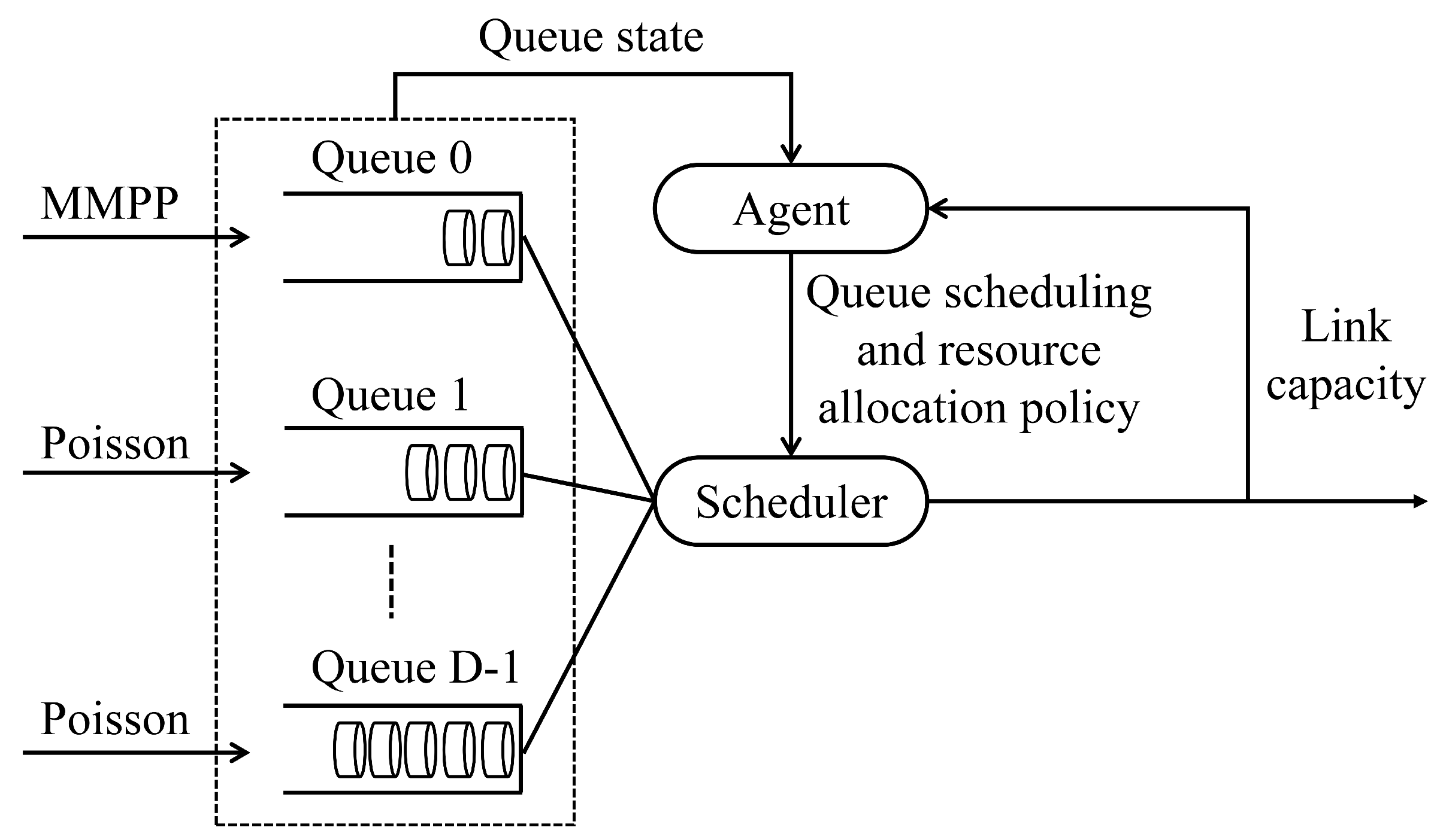
Figure 2.
Basic architecture of CSAC-HQS.
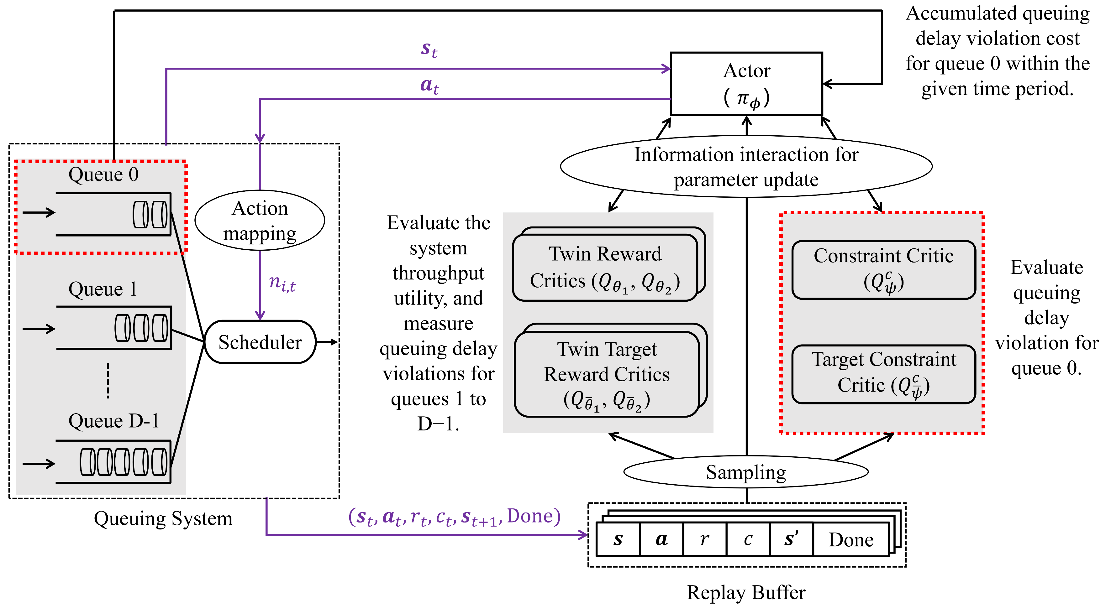
Figure 3.
Queuing delay violation rate of queue 0 with a maximum allowable queuing delay of 10 ms (2 time slots).
Figure 3.
Queuing delay violation rate of queue 0 with a maximum allowable queuing delay of 10 ms (2 time slots).
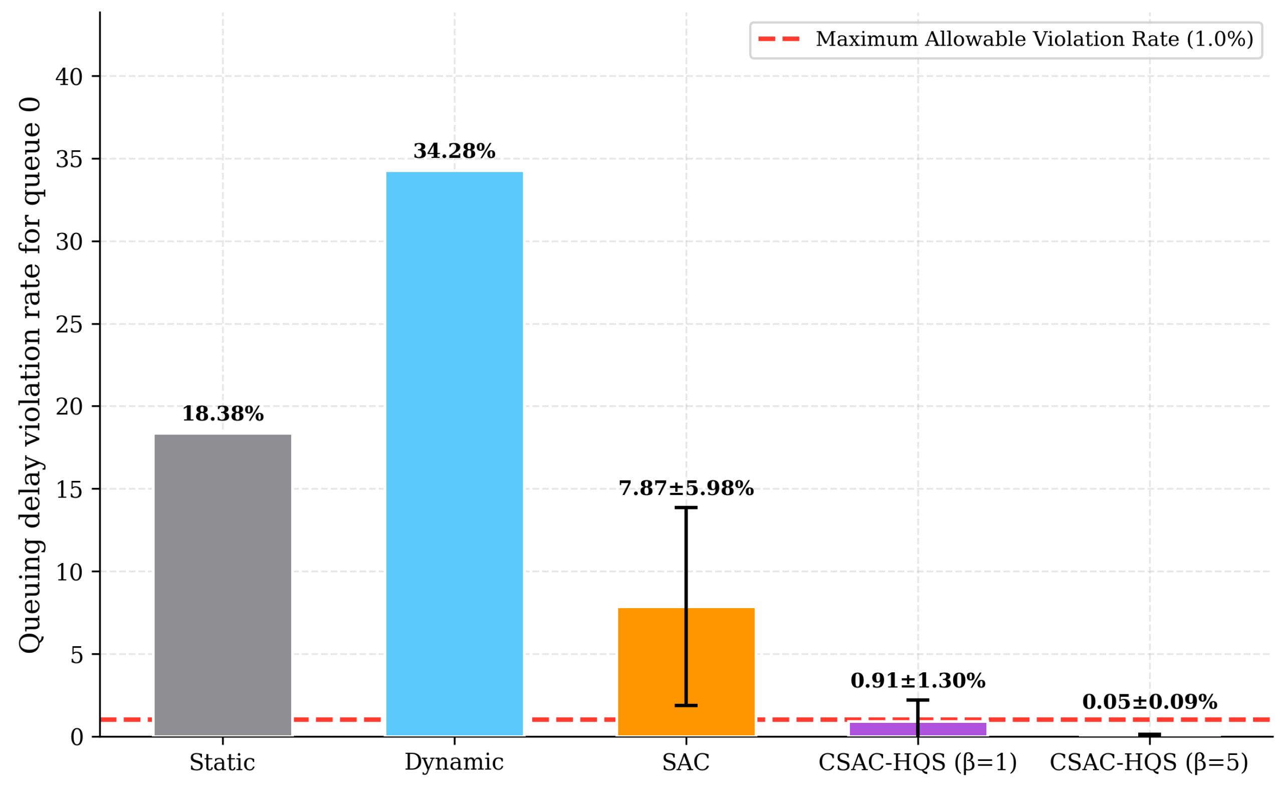
Figure 4.
Average queuing delay of the best-effort queues (queues 1 and 2), with maximum allowable queuing delays of 20 ms and 30 ms, respectively.
Figure 4.
Average queuing delay of the best-effort queues (queues 1 and 2), with maximum allowable queuing delays of 20 ms and 30 ms, respectively.
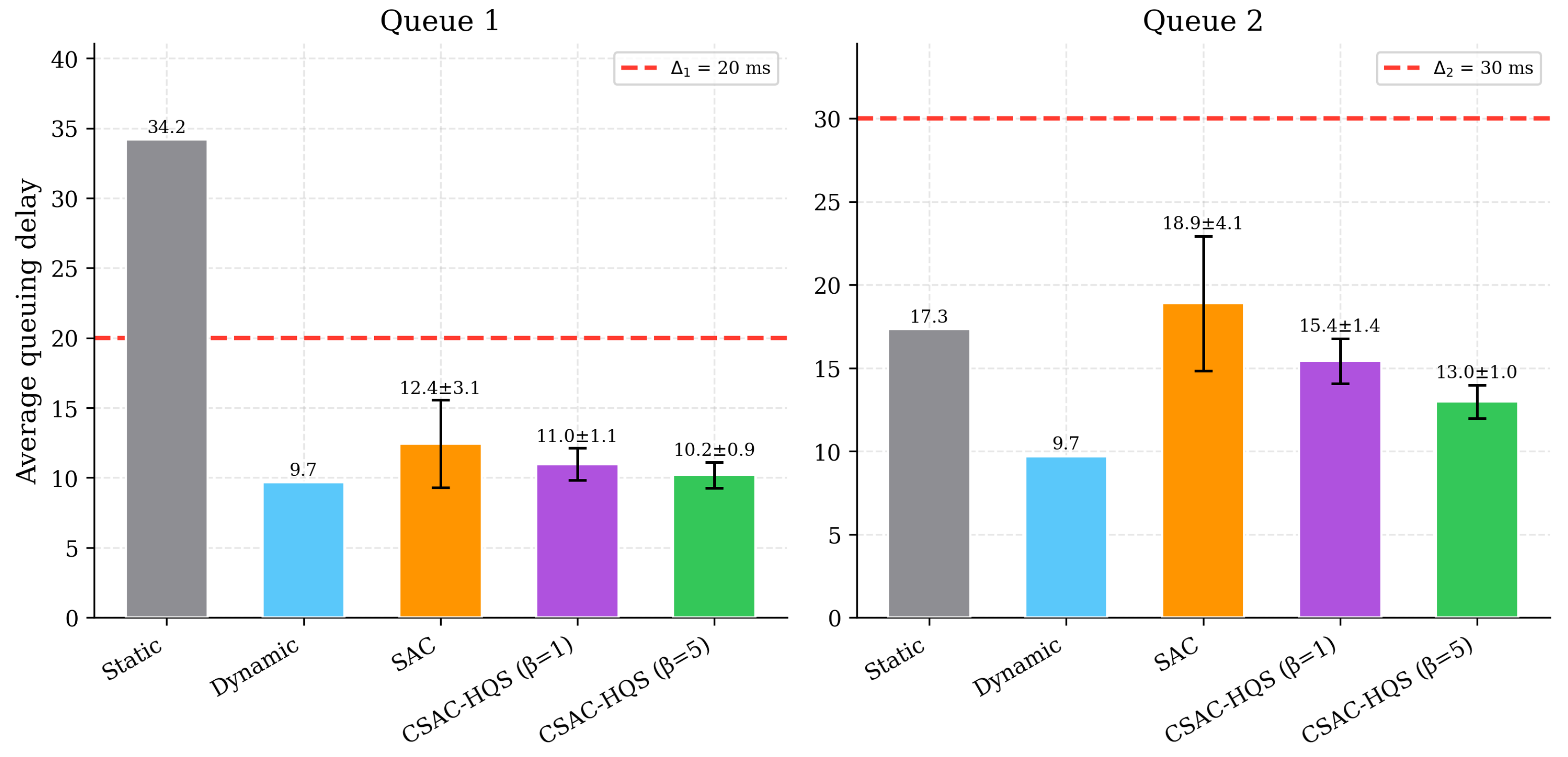
Figure 5.
Throughput and overflow packet count per queue.
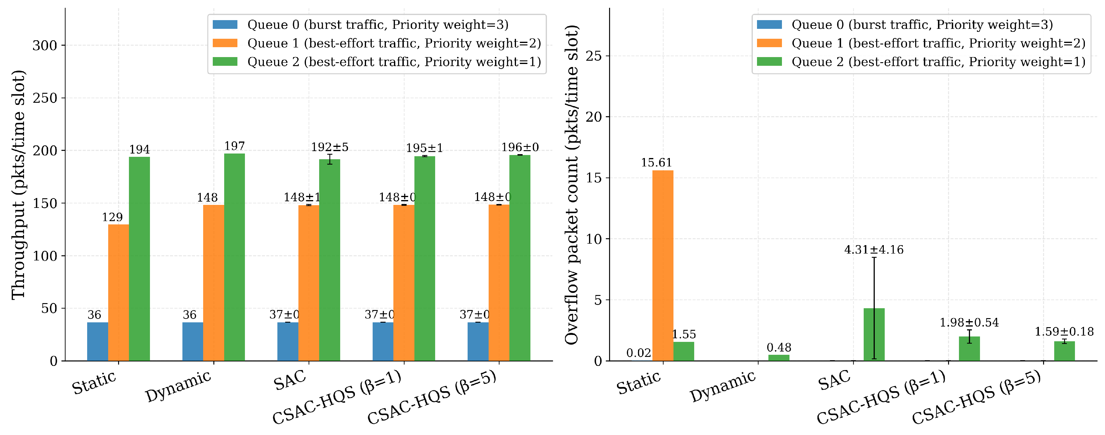

Table 1.
Queuing system configurations and CSAC-HQS hyperparameters.
| Category | Parameter | Value |
|---|---|---|
| Queuing System | Number of queues (D) | 3 |
| Buffer capacity (B) | 1000 packets | |
| Time slot duration () | 5 ms | |
| Episode length (H) | 200 time slots | |
| Link capacity lower bound () | 338 packets | |
| Link capacity upper bound () | 438 packets | |
| Maximum allowable queuing delays for queue 0, 1, 2 () | 10, 20, 30 ms | |
| MMPP transition probabilities of queue 0 (, ) 1 | , | |
| MMPP normal and burst arrival rates | 5, 20 packets/ms | |
| Arrival rates of queue 1, 2 | 30, 40 packets/ms | |
| CSAC-HQS | Optimizer | Adam |
| Optimizer learning rate | ||
| Discount factor () | 0.99 | |
| Replay buffer size | ||
| Mini-batch size (N) | 256 | |
| Soft-update coefficient () | 0.005 | |
| Entropy temperature () | auto-tuned, initialized at 0.2 | |
| Total training steps | ||
| Actor hidden layers | [64, 64, 64, 64] | |
| Critic hidden layers | [128, 128, 128, 128] | |
| Sharpening factor () | 1, 5 | |
| History window of the link capacity () | 10 time slots | |
| Warm-up steps () | 1000 time slots | |
| Update interval (G) | 10 time slots | |
| Gradient steps per update | 1 | |
| Per-episode queuing delay violation budget () | 2 | |
| Multiplier learning rate () | ||
| Entropy temperature learning rate () | ||
| Maximum multiplier () | 5 | |
| Reward-scaling coefficient () | 0.01 | |
| Priority weights () | ||
| Throughput utility coefficient () | 1.0 | |
| Queuing delay violation penalty coefficient () | 1.0 | |
| Drop penalty coefficient () | 0.5 | |
| Queuing delay violation penalty clip multiplier () | 10 |
1 is the transition probability from state 0 to state 1 and is the reverse, where states 0 and 1 denote normal and burst modes, respectively.
Table 2.
Configurations of the learning-based methods.
| SAC | CSAC-HQS | |
|---|---|---|
| Sharpening factor | 1 | 1, 5 |
| Masked-softmax | yes | yes |
| Queuing delay violation penalty indicator of queue 0 () | 1 | 0 |
| Queuing delay violation penalty indicator of queue 1 () | 1 | 1 |
| Queuing delay violation penalty indicator of queue 2 () | 1 | 1 |
| Constraint critic | — | yes |
| Lagrangian update on | — | yes |
| Warm-up steps | 1000 | 1000 |
Disclaimer/Publisher’s Note: The statements, opinions and data contained in all publications are solely those of the individual author(s) and contributor(s) and not of MDPI and/or the editor(s). MDPI and/or the editor(s) disclaim responsibility for any injury to people or property resulting from any ideas, methods, instructions or products referred to in the content. |
© 2026 by the authors. Licensee MDPI, Basel, Switzerland. This article is an open access article distributed under the terms and conditions of the Creative Commons Attribution (CC BY) license (http://creativecommons.org/licenses/by/4.0/).
Copyright: This open access article is published under a Creative Commons CC BY 4.0 license, which permit the free download, distribution, and reuse, provided that the author and preprint are cited in any reuse.